the Creative Commons Attribution 4.0 License.
the Creative Commons Attribution 4.0 License.
 | 02 Dec 2020
Improved cloud detection over sea ice and snow during Arctic summer using MERIS data
Henrik Marks
Marcus Huntemann
Georg Heygster
Gunnar Spreen
The historic MERIS (Medium Resolution Imaging Spectrometer) sensor on board Envisat (Environmental Satellite, operation 2002–2012) provides valuable remote sensing data for the retrievals of summer sea ice in the Arctic. MERIS data together with the data of recently launched successor OLCI (Ocean and Land Colour Instrument) on board Sentinel 3A and 3B (2016 onwards) can be used to assess the long-term change of the Arctic summer sea ice. An important prerequisite to a high-quality remote sensing dataset is an accurate separation of cloudy and clear pixels to ensure lowest cloud contamination of the resulting product. The presence of 15 visible and near-infrared spectral channels of MERIS allows high-quality retrievals of sea ice albedo and melt pond fraction, but it makes cloud screening a challenge as snow, sea ice and clouds have similar optical features in the available spectral range of 412.5–900 nm.
In this paper, we present a new cloud screening method MECOSI (MERIS Cloud Screening Over Sea Ice) for the retrievals of spectral albedo and melt pond fraction (MPF) from MERIS. The method utilizes all 15 MERIS channels, including the oxygen A absorption band. For the latter, a smile effect correction has been developed to ensure high-quality screening throughout the whole swath. A total of 3 years of reference cloud mask from AATSR (Advanced Along-Track Scanning Radiometer) (Istomina et al., 2010) have been used to train the Bayesian cloud screening for the available limited MERIS spectral range. Whiteness and brightness criteria as well as normalized difference thresholds have been used as well.
The comparison of the developed cloud mask to the operational AATSR and MODIS (Moderate Resolution Imaging Spectroradiometer) cloud masks shows a considerable improvement in the detection of clouds over snow and sea ice, with about 10 % false clear detections during May–July and less than 5 % false clear detections in the rest of the melting season. This seasonal behavior is expected as the sea ice surface is generally brighter and more challenging for cloud detection in the beginning of the melting season.
The effect of the improved cloud screening on the MPF–albedo datasets is demonstrated on both temporal and spatial scales. In the absence of cloud contamination, the time sequence of MPFs displays a greater range of values throughout the whole summer. The daily maps of the MPF now show spatially uniform values without cloud artifacts, which were clearly visible in the previous version of the dataset.
The developed cloud screening routine can be applied to address cloud contamination in remote sensing data over sea ice.
The resulting cloud mask for the MERIS operating time, as well as the improved MPF–albedo datasets for the Arctic region, is available at https://www.seaice.uni-bremen.de/start/ (Istomina et al., 2017).
- Article
(6783 KB) - Full-text XML
- BibTeX
- EndNote


No other surface type of satellite imagery has the unique features of bright, reflecting white snow surface. The task of snow detection therefore would be an easy task in the absence of clouds. However, the snow spectral signature (e.g., Warren, 1982) is also a feature of water and especially of ice clouds (Kokhanovsky, 2006). Possible snow impurities, snow grain size differences and liquid water content create fine differences between many snow types (Warren, 1982), but in general the spectra of snow and cloud are similar in the visible and near infrared, with the difference occurring beyond 1 µm (e.g., channels at 1.6, 3.7, 11 and 12 µm).
For MERIS data with a spectral range from 412.5 to 900 nm, cloud detection over snow and sea ice is a challenging task. However, the advantage of MERIS – its 15 spectral bands within this relatively small spectral range – makes it especially suitable for the melt pond fraction (MPF) retrieval over the Arctic sea ice, which needs a quality cloud screening routine.
Although most of the field campaigns and in situ measurements of the sea-ice-covered Arctic ocean are performed during Arctic summer (e.g., an overview in Istomina et al., 2015), the links and feedbacks between the rapidly evolving sea ice surface, the atmosphere and the under-ice ecosystem are multifold (Curry et al., 1996) and not yet fully understood. The appearance of melt ponds on sea ice during melt onset causes a drastic change of its albedo and transmittance (Nicolaus et al., 2012) which affects the surface energy balance and facilitates lateral, top, bottom and internal sea ice melt, i.e., affects the sea ice volume. Only recently the suggestion that melt ponds during melt onset might be connected to the sea ice area during the sea ice minimum has been published (Schröder et al., 2014). In order to understand these processes, a long-term global coverage record of sea ice parameters, among others also MPF, needs to be available to the community. That is, the presented cloud screening routine and the resulting MPF dataset can be used in studies of sea ice processes and feedbacks.
To the knowledge of the authors, at the time of writing no climate model includes melt ponds on top of sea ice. One of the reasons is that melt ponds, although observed in situ during many campaigns, still present a challenge for climate modeling due to unknown global spatial distribution. Although reanalysis air temperature at the surface is also available over sea-ice-covered Arctic ocean (e.g., Kalnay et al., 1996), MPF is not linearly linked to the air temperature but also depends on the ice topography and its internal macrophysical properties such as density, porosity, etc. Satellite MPF datasets of possibly global coverage are the only way to understand not only local events but also global spatial dynamics, which may eventually lead to successful inclusion of melt ponds into climate models.
Besides cloud screening for the MPF retrieval using MERIS data, a robust cloud detection from MERIS in the Arctic region may be important for (1) synergy with the other sensors on board Envisat and (2) might be applicable to sensors similar to MERIS, e.g., OLCI.
The cloud screening for OLCI, which is a successor of MERIS without thermal infrared bands, presents challenges similar to those of MERIS. OLCI data are important as a continuation of MERIS in order to provide long-term data records of, for example, MPF. Nevertheless, the cloud screening presented here has been developed specifically for MERIS and thus addresses the issue of cloud screening over snow for ENVISAT sensors, e.g., SCIAMACHY (SCanning Imaging Absorption spectroMeter for Atmospheric CHartographY; see e.g., Schlundt et al., 2011). Of course, the approach presented here can be applied to OLCI data as well.
Depending on the retrieved parameter and sensor, the effect of a compromised cloud screening may be moderate (retrievals of albedo and snow grain size within SGSP, snow grain size and pollution amount retrieval; Wiebe et al., 2013) to drastic (aerosol retrieval, Istomina et al., 2011; MPF retrieval, Zege et al., 2015). As the melting sea ice displays a variety of spectral behaviors in the entire range from white ice to dark melt ponds (e.g., Istomina et al., 2013), a versatile forward model and retrieval which can account for such a variability at a global spatial scale are needed. Such a retrieval (melt pond detector, MPD) has been developed by Zege et al. (2015). The MPD is a pixelwise retrieval and only utilizes the spectral information without additional morphological or statistical criteria. As clouds do not spectrally differ from most of the surfaces available during Arctic summer, so that, for example, warm water clouds may appear similar to white ice throughout most of the available spectral range (same for cirrus and fresh fine snow), the MPD can therefore misinterpret the cloud contamination as sea ice melt. The resulting MPF and albedo datasets are thus strongly affected by the residual cloud contamination. The objective of this work is to resolve this issue by means of a reliable cloud discrimination over snow for MERIS and to provide the datasets of MPF, albedo and cloud mask of a better quality than currently available.
Some sensors are better suited for the task of cloud screening but are not suitable for the MPD retrieval due to other limitations. For example, the MODIS cloud mask (Ackermann et al., 1998; Liu et al., 2004) is one of the most comprehensive classification algorithms; however, as the MODIS sensor experiences saturation in some of the visible bands (Madhavan et al., 2012), it is impossible to use these data for the given sea ice albedo and MPF retrieval (Zege et al., 2015). As the MERIS sensor on board Envisat does not have these limitations, it has been chosen for the retrievals of MPF and albedo. However, the choice of methodology to perform cloud screening over snow and ice with MERIS is not a trivial task.
Three basic cloud-screening approaches applicable to a spectroradiometer data can be distinguished among the available algorithms.
-
Analyze time sequences of data, under the assumption that the short-term changes of the scene can only be introduced by clouds (e.g., Key and Barry, 1989; Diner et al., 1999; Lyapustin et al., 2008; Lyapustin and Wang, 2009; Gafurov and Bárdossy, 2009). Such an approach assumes surfaces with a constant and pronounced structure (Lyapustin et al., 2008; Lyapustin and Wang, 2009). Although the approach proved to be effective for various natural and artificial surfaces, it is not applicable within this work due to the fast-evolving nature of melt ponds and the sea ice.
-
Apply a reflectance or brightness temperature absolute threshold or their combination, e.g., ratio of reflectances in the form of normalized difference vegetation index (NDVI). In this case, only a few channels are used (e.g., Minnis et al., 2001; Bréon and Colzy, 1999; Lotz et al., 2009; Allen et al., 1990; Spangenberg et al., 2001; Trepte et al., 2001). The optical properties of snow in the visible spectral range show weak spectral dependency. In the near infrared and infrared, however, the snow spectrum shows the typical “snow signature”, i.e., values decreasing due to water absorption in the near infrared, which also causes the dependence on the snow grain size due to different path length and absorption in the grains of different size. These features aid the snow–cloud discrimination. Therefore, it is a common practice to use infrared channels in addition to the visible for such retrievals (Spangenberg et al., 2001). In the current task, the limited spectral range of MERIS does not allow effective usage of this approach.
-
Analyze image processing and spatial variability (e.g., Martins et al., 2002). In the case of white clouds over white surface, the spatial variability would mainly come from the difference in grain/particle size, surface roughness, different water phase (ice surface vs. water cloud, melting surface vs. ice cloud) and cloud shadows. Given the great natural variability of these parameters in both Arctic clouds and surface and the similarity of their optical properties in the given spectral range, this approach is prone to false detections.
Combinations of the above methods together with additional thresholds and additional meteorological/reanalysis data are also available. For example, the MODIS cloud detection scheme (Ackerman et al., 1998; Liu et al., 2004) is one of the most comprehensive among the available cloud detection schemes and is based on such a combination. This algorithm uses 19 out of 36 MODIS channels along with additional inputs, e.g., topography and illumination observation geometry for each 1 km pixel, land–water mask, ecosystem maps and daily operational snow–ice products (taken from the NOAA, National Oceanic and Atmospheric Administration and NSIDC, National Snow and Ice Data Center). The resulting MODIS cloud mask contains four confidence levels (confident cloudy, uncertain, probably clear, confident clear) and is available as a separate daily averaged product. Unfortunately, due to the time lag between Envisat and Terra–Aqua, the MODIS cloud mask product cannot be used for swathwise screening for the melt pond fraction retrieval.
Most of the cloud screening approaches do not focus on the case of the snow surface; among those who do (Allen et al., 1990; Spangenberg et al., 2001; Trepte et al., 2001; Istomina et al., 2010, 2011), even a smaller fraction utilizes MERIS sensor for this task (Kokhanovsky et al., 2009; Schlundt et al., 2011; Zege et al., 2015; Istomina et al., 2015; Krijger et al., 2011).
The currently available cloud masks for MERIS (Zege et al., 2015; Schlundt et al., 2011, etc.) are based on NDSI-like (normalized difference snow index) indices, e.g., MDSI (MERIS Differential Snow Index). In the absence of infrared channels these thresholds result in a residual cloud contamination over snow and sea ice. However, unlike most of the moderate resolving spectroradiometers, MERIS has the so-called oxygen A band (MERIS channel 11 at 761.5 nm), which can aid greatly in cloud screening over snow and ice.
MERIS oxygen A band and the smile effect
As oxygen is well mixed in the Earth atmosphere, the amplitude of absorption within MERIS channel 11 reflects optical path length of light rays received with the sensor. Effective path length over clouds is shorter than that over sea ice or snow on land; that is, light reflected from clouds experiences less absorption when traveling through the atmosphere than light reflected from the surface. This allows the separation of clouds and snow or sea ice surface according to their height in the atmospheric column. We expect this criterion to work best for optically thick water clouds. The sensitivity to optically thin clouds is expected to be small over bright surfaces like sea ice (Preusker and Lindstrot, 2009), and clouds with a low top height would generally also have a weaker effect on the oxygen ratio. Fortunately, as in our case the Arctic sea ice surface lies uniformly at sea level and displays no relief, there is no confusion possible between clouds and surface in the terms of optical path length, and the only uncertainty might come from the sensor-specific features, i.e., the smile effect. As MERIS is a push-broom sensor, its channels are susceptible to the smile effect usual for this type of sensor, which occurs due to a small variation in the central wavelength across the MERIS swath. The artifacts appear as along-track stripes within the swath and impair application of thresholds or retrievals. The oxygen ratio approach without the smile correction has been used by Zege et al. (2015) and Istomina et al. (2015) as a threshold in addition to classical whiteness and brightness criteria. The threshold comprises the ratio of 11 (oxygen A absorption) and 10 (oxygen A reference) R11∕R10 < 0.27, where the value 0.27 has been derived from the visual analysis of several dozen MERIS scenes (see Zege et al., 2015, and Eq. 17 therein). As seen in Zege et al. (2015) and Istomina et al. (2015), strong artifact presence compromises the effective application of the oxygen ratio threshold.
The smile effect of MERIS has been studied (Bourg et al., 2008), and ways to correct it have been shown by Gómez-Chova et al. (2007) or Jäger (2013). The approach by Jäger (2013) greatly improves the usability of the oxygen ratio but does not fully remove detector-to-detector differences. A reason for this might be instrument stray light, which is not fully removed in the MERIS operational processing chain (Lindstrot et al., 2010), and that was not taken into account by Jäger (2013).
Another available smile effect, corrections also comprise those included in the ESA (European Space Agency) toolbox for Envisat processing, i.e., open-source packages BEAM or SNAP (Earth Observation Toolbox and Development Platform, Sentinels Application Platform, https://www.brockmann-consult.de, last access: 30 July 2020). These corrections work well within the transparency window of the atmosphere over darker surfaces but are not sufficient in the oxygen A absorption band over brighter surfaces such as snow and ice.
In this work, we suggest a smile correction for MERIS band 11 which allows slight inaccuracy on the absolute value of the top-of-atmosphere (TOA) reflectances but preserves the relative difference between the sensor pixels, which allows a quantitative use of the corrected oxygen A band for cloud screening (Sect. 3.3.1).
The cloud screening method for MERIS data developed in this work is specifically aimed to work well over summer sea ice. It is called MECOSI (MERIS Cloud screening Over Sea Ice). MECOSI utilizes the collocated AATSR data in the center part of the MERIS swath, namely the infrared channels 1.6, 3.7, 11 and 12 µm, for training. In this work, we use the AATSR cloud screening developed for the aerosol retrieval over snow and ice (Istomina et al., 2010).
Currently MECOSI is being applied as preprocessing for the retrieval of melt pond fraction and spectral albedo of summer sea ice (MPD). The MPD retrieval takes top-of-atmosphere reflectances of MERIS at nine channels as input and employs a forward model of optical properties of the Arctic surface and an iterative procedure to retrieve spectral albedo and melt pond fraction of a given pixel. Several hundred field spectra of the Arctic sea ice and melt ponds have been used to constrain the input parameters of the forward model and to ensure realistic range of modeled surfaces. More details on the MPD retrieval can be found in Zege et al. (2015). The presented cloud screening method can be used for other remote sensing applications as well, e.g. for retrievals of other surface or atmospheric parameters or as a cloud mask for coarser resolving sensors on board same satellite platform (e.g., SCIAMACHY on Envisat).
3.1 Data used
Input for MECOSI is MERIS Level 1B observations. MERIS consists of five cameras scanning the surface of the Earth in push-broom mode and offers 15 spectral bands from 412.5 to 900 nm. The data are collected globally with a spatial resolution of 1040 m × 1200 m at nadir. The Level 1B product provides calibrated and georeferenced TOA radiances. These are preprocessed using the software package BEAM (http://www.brockmann-consult.de/cms/web/beam/, last access: 30 July 2020).
The preprocessing includes the following.
-
The region north of 65∘ N is cut out from each orbit using the module subset.
-
The metadata in the L1B swaths are given in a grid with reduced resolution and need to be interpolated in order to have the data available for each pixel. This is done using the BandMath module. The coordinates as well as sun zenith and the view zenith angles are now interpolated.
-
The TOA radiances are corrected and converted to reflectances using the module Meris.CorrectRadiometry. The correction includes an equalization step to reduce detector-to-detector differences and a scheme to reduce the smile effect in all but the absorption bands 11 and 15.
A cloud mask derived from AATSR data (Istomina et al., 2010) is used as a reference mask to develop and validate the MECOSI algorithm. The AATSR instrument has been launched together with MERIS aboard Envisat, and both sensors observe the same scene nearly simultaneously. The spatial resolution of AATSR is 1 km at nadir, which is similar to the spatial resolution of MERIS. However, as AATSR has a narrower swath of 512 km, it covers only the central half of a MERIS swath. The AATSR cloud-screening algorithm has been developed for an aerosol optical thickness retrieval and is presented by Istomina et al. (2010). It exploits knowledge about the spectral shape of snow in visible, near-infrared and thermal infrared bands of AATSR. As intercomparisons of cloud-screening routines are challenging due to the time difference between the overflights of different satellite sensors, the validation has been performed against in situ lidar data. The comparison of the AATSR cloud mask to the micro-pulse lidar data has proven the robustness of the method (95 % correct cloudy and clear detections with the remaining 5 % of cases connected to thin clouds on a sample of ∼ 100 scenes). The output is a binary mask for cloud-free snow and ice.
The training dataset used in this work was prepared as follows: all AATSR swaths from May to September 2009, 2010 and 2011 have been subset, transformed into TOA and co-located to the corresponding MERIS swaths using a nearest-neighbor algorithm (radius of influence 1.5 km). As the AATSR and MERIS data have different spatial resolutions, the two datasets have been gridded to a single grid (the coarser grid of MERIS). This might have affected the pixels at the borders of clouds in a way that earlier fully covered pixels now become partly covered, which the binary AATSR cloud mask cannot fully reflect. Therefore we exclude the two-pixel border from the study.
This AATSR dataset from May to September 2009–2011 was used to estimate the cloudy and clear case probabilities for the given feature vector as described in the next sections.
3.2 Bayesian cloud screening
A comprehensive introduction to the theory of Bayesian cloud screening is given by Hollstein et al. (2015). The described approach can be found in detail in Marks (2015). In the following, P(A,B) denotes the occurrence probability of A under the condition that the occurrence of B and F is a vector of features derived pixelwise from satellite data. If C denotes cloudy conditions ( – clear conditions), the probability of seeing a cloudy pixel under the occurrence of F can be written as
Using this equation to calculate the cloud probability P(C,F), we need to estimate the probabilities P(F,C) and for each possible feature vector F∈RN. We accomplish this by calculating N-dimensional frequency histograms, one for cloud and one for clear-sky cases as flagged in the AATSR mask. This is done for every AATSR and MERIS swath for the time period 1 May to 30 September 2009. The background probability P(C) is directly calculated from the AATSR masks using data from the same year. Pixels outside the AATSR swath are not used in this analysis. The set of features for which the above procedure is being performed is described below.
3.3 Features and applied corrections
The selection of the features used to build the feature vector F is the most important step during the development of the algorithm and greatly affects the performance of the screening. Hollstein et al. (2015) used a random search algorithm to find a set of features Fi that performs best in global application. Here, however, the features are selected manually to find a set that performs best over snow-covered ice and darker, ponded ice. Additionally, correction algorithms were developed to equalize the systematic dependencies on the cross-track pixel position.
3.3.1 Oxygen A ratio
The TOA ratio of the oxygen A band 11, which is located at the oxygen absorption line at 761 nm, to band 10 at 754 nm, which is the oxygen reference band, is used here to estimate the absorption by oxygen in the atmospheric column above the reflecting surface:
The ratio rox cannot be used directly in the feature vector F because of dependencies on the illumination–observation geometry and because of the smile effect artifacts. The optical path through the atmosphere depends on sun and view zenith angles in both cloudy and clear cases and needs to be accounted for. As these angles are provided in MERIS Level 1B swath data, the air mass factor can be calculated (e.g., Gómez-Chova et al., 2007). The smile effect artifacts in rox need additional consideration before it can be used for cloud screening.
In this work, we propose an empirical approach to equalize rox and decrease the influence of the abovementioned factors across the swath. We assume that over a statistically significant sample, the mean value of rox for a given set of conditions (e.g., for a given detector index, geometry) can be used to correct the systematic across-track dependence for this set of conditions. We assume that rox depends on three parameters: the detector index Id which corresponds to the position of the pixel in the detector array, the sun zenith angle θs and the viewing zenith angle θv. Id gives a pixel's position in the sensor array and allows compensation for the spectral smile effect. The sun zenith angle θs and the viewing angle θv allow the estimation of the optical path in the atmosphere which is directly dependent on the oxygen absorption. The seasonal nature of rox dependence on surface reflectance, for example, at channel 779 nm presents a challenge of statistically non-uniform bins of vastly different sample sizes and was not included in the correction scheme. The residual rox dependence on the surface reflectance is less than 2 % (Fig. 2) and does not prevent the application of the cloud screening routine. Assuming , we obtain a set of data vectors:
The set I denotes the indices of all pixels in one swath. Pixels with the same detector index Id are selected from the set M and corresponding subsets are built:
These subsets Mj are then processed separately. The ratio is binned as follows:
The bin width δ is set to 1∕4∘. The sets are calculated for many swaths K, typically all summer data of 1 year. Then the mean value of rox is calculated for each one of these sets:
Finally, a fifth-order polynomial is fitted to the averaged values for each separate detector index j to achieve smooth and continuous correction functions fj:
which in addition are functions of θsum. The correction is applied pixelwise by evaluating f and subtracting the resulting value from the oxygen A ratio. The corrected ratio is then used as a feature in the cloud screening algorithm.
It must be noted that as the further calculation of cloud probabilities for the given detector indices and values of rox happens in the space of corrected rox only, the absolute amplitude of rox is not important for our application and is not preserved within the described approach. Instead, the relative difference between the scattering events at the surface and at the cloud are equalized throughout the swath and thus made available for cloud screening.
The above-described approach has been performed over all MERIS swathes to above 65∘ N for the time range from 1 May to 30 September 2009. This sample is considered to be statistically significant in terms of variety of surface and cloud types and their seasonal behavior under a variety of observation–illumination geometries for all detector indices.
3.3.2 MERIS Differential Snow Index
The MERIS Differential Snow Index (MDSI) is defined as normalized difference of the TOA reflectances at 865 and 885 nm:
It exploits the drop in spectral reflectance of snow and ice at the given wavelengths to aid discrimination of snow and ice from clouds (Schlundt et al., 2011). The systematic cross-track variation is less pronounced than that for the oxygen A ratio, and no dependence on the observational geometry is expected; i.e., it is assumed to be the same for both spectral bands R13 and R14. Therefore, we use a simplified correction scheme: the mean value of Fsi is calculated for each detector index using swaths from the summer 2009. Open-water pixels have been removed using two thresholds on channels 12 and 13 as described by Schlundt et al. (2011). As before, to remove the systematic across-track variability, the obtained mean values are subtracted from Fsi for each detector index.
3.3.3 Brightness and whiteness
Many types of clouds have a higher reflectance than snow in the near infrared and they usually show a white spectrum. The usefulness of these two features to detect clouds has been shown in Gómez-Chova et al. (2007) and the same definitions are used here. The brightness b is a spectral integral over the reflectance. As the spectral resolution of the sensor is quite coarse with only 13 used channels, the brightness can be represented by the following equation:
Here, λ denotes the center wavelength of a MERIS band and I is the set of used bands. The absorption bands 11 and 15 are excluded from the calculation; hence, we use bands 1–10 and 12–14 to calculate the overall brightness b. The whiteness w of the spectrum is measured by the deviation of the radiances from the brightness b. With , the equation is
Note that small values for w correspond to a flat and therefore white spectrum.
3.4 Evaluation
The cloud probabilities for each given set of features (Sect. 3.2) were compiled into binary masks in order to compare the results to the binary AATSR cloud masks. The masks are created by normalizing the cloud probability P(F,C) to the range [0,1] and splitting the dataset at a probability threshold of 0.45 to introduce binary values. An operation of morphological closing and opening was then applied to the cloud and snow or sea ice pixels in order to remove single pixels. The binary MECOSI and AATSR cloud masks are used to filter out clouds in the MPD swath data. No co-location or interpolation is necessary for this step because both algorithms, the MECOSI cloud screening and MPD, process identical MERIS swaths, and the AATSR cloud masks were gridded to the MERIS grid. The comparison of the three cloud masks, as well as illustration of separate features of the feature vector F as well as their corrections, is given in the next section.
4.1 Oxygen A correction
An example of the influence of the oxygen A correction described in Sect. 3.3.1 is presented in Fig. 1. The jumps at the transition between the five detectors of MERIS, visible as vertical stripes in the uncorrected ratio (Fig. 1b), are strongly reduced by applying the correction (Fig. 1c). The influence of low sun elevation, which causes the dark top left corner in the uncorrected ratio, is much less apparent. Also, there are no pronounced artifacts introduced by the discrete look-up table (Sect. 3.3.1) used for the correction, as the corrected ratio is a rather smooth image. Very bright pixels, e.g., cloud edges visible in Fig. 1a, are darker and more apparent after applying the correction.
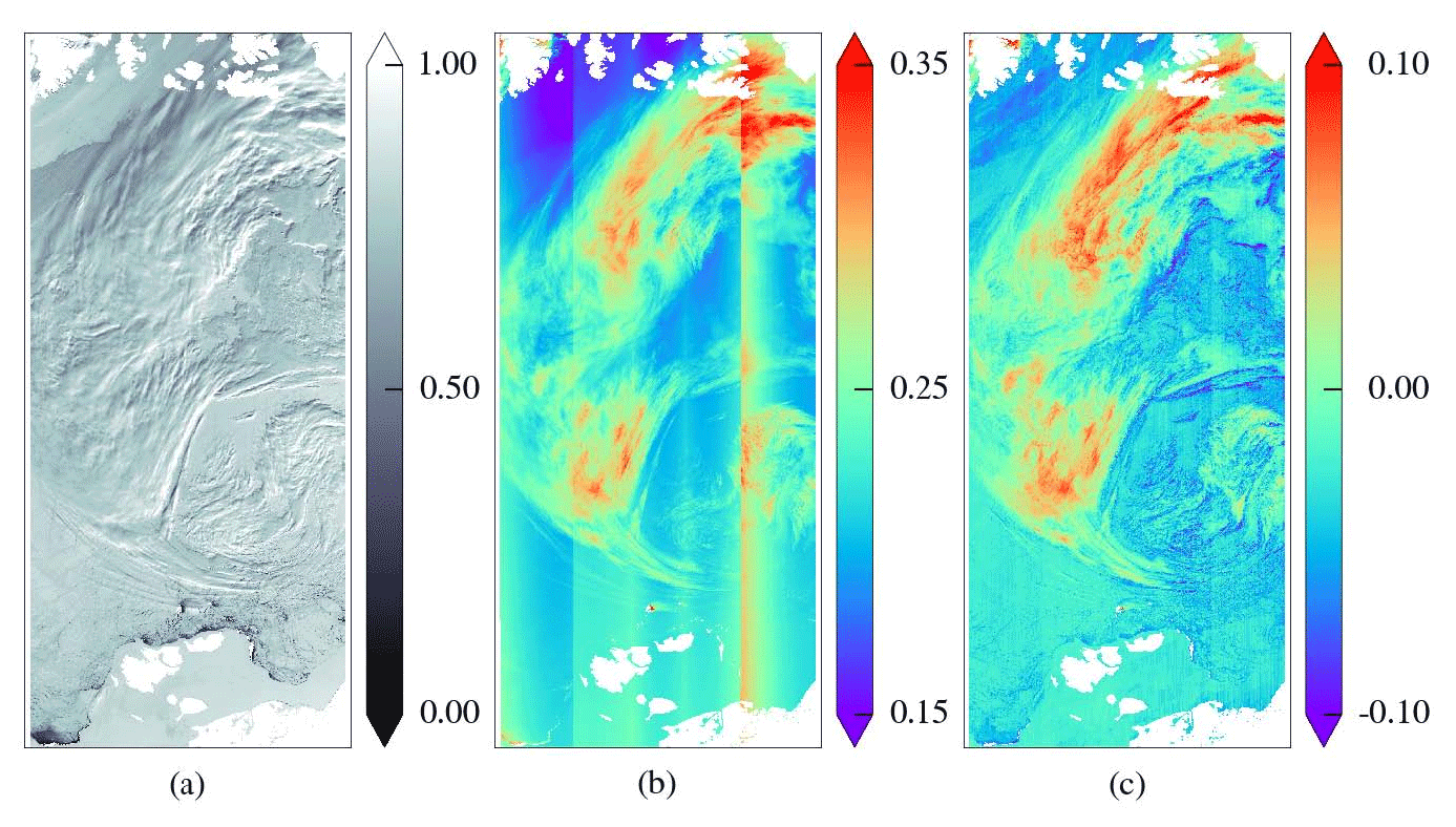
Figure 1Reflectance at 779 nm (a), uncorrected oxygen A ratio (b) and corrected oxygen A ratio used as a feature in the cloud screening (c). Shown is a 2450 × 1121 pixel part of Envisat orbit 37475 from 1 May 2009 with the New Siberian Islands at the bottom and parts of the Canadian Archipelago at the top. Land, open water and invalid pixels are white.
Another way to investigate the effect of the correction is to study the along-track mean of the oxygen A ratio. As expected, the corrected ratio is a smooth function with values close to zero, if data from the whole period May to September are considered (Fig. 2 black line). This is different for the data from May only, where we find small jumps between the detectors (Fig. 2 red line). Moreover, there is a negative slope in the along-track mean, which implies that pixels at the right side of the swath tend to be darker than the ones on the left side. For the data of July, we find a reverse sign situation (Fig. 2, blue line). This seasonal dependence is expected due to the illumination–observation geometry change in the course of summer; however, these artifacts are minimal and still allow a high-quality cloud detection using the oxygen A MERIS band.
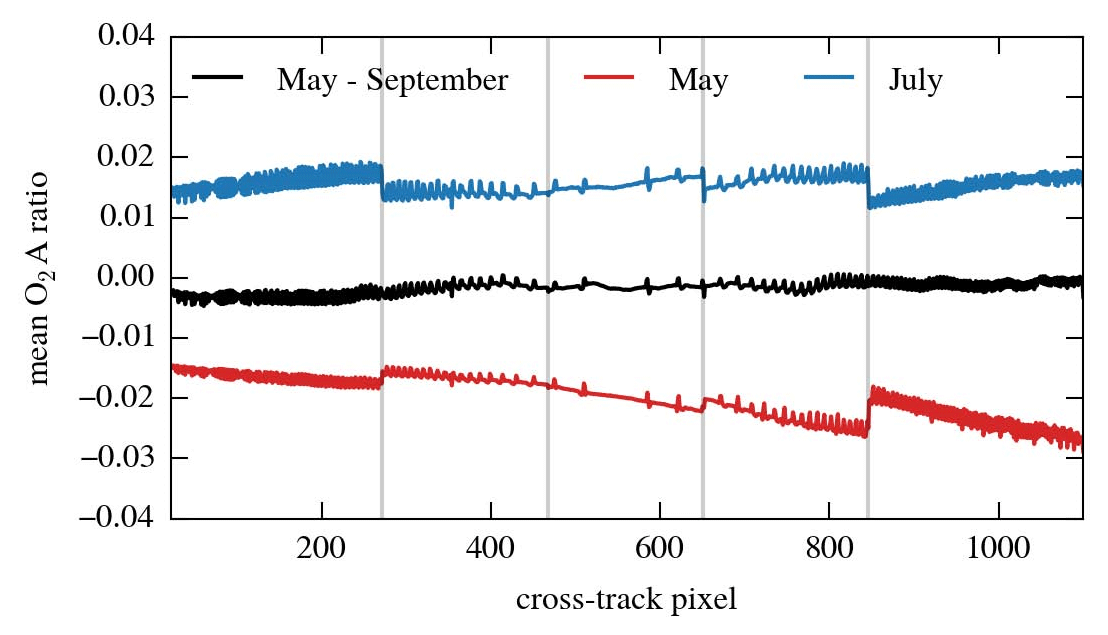
Figure 2Along-track mean of the corrected oxygen A ratio. For each time period, the mean is calculated from 100 randomly selected swaths. The vertical lines mark the transition between the five detectors of MERIS.
4.2 Comparison to AATSR cloud mask
We first investigate whether the MECOSI algorithm can reproduce the AATSR cloud mask for the year 2009 used for the algorithm training. As AATSR data also contain thermal infrared bands, in which the snow and ice surface is virtually a blackbody, the cloud detection with AATSR shows good reliability in the Arctic (Istomina et al., 2010) and can be used as a reference in this study. Figures 3 and 4 show two examples of the MECOSI cloud probability, one for the typical situation at the beginning of the melt season in May with bright, snow-covered ice (Fig. 3) and one for darker, ponded ice at the peak of the melt season in July (Fig. 4). In both cases, the cloud probability (Figs. 3b and 4b) corresponds to the AATSR mask (Figs. 3c and 4c). Most clouds visible in the TOA reflectance images (Figs. 3a and 4a) are prominent with significantly higher cloud probabilities. No distinct difference in cloud probability is visible across the swath and dependencies on the acquisition geometry or detector-specific properties appear to be well compensated. However, closer inspection reveals several cases of false negatives, like the semitransparent clouds over landfast ice which cannot be discriminated from clear-sky regions by their cloud probability (red arrow in Fig. 3a). The opposite case is shown with a blue arrow in Fig. 3a, where low ice concentrations close to the coast were falsely detected as high cloud probability.

Figure 3Reflectance at 779 nm (a), cloud probability (b) and corresponding AATSR mask (c) for 14 May 2009 with Svalbard at the bottom left corner. Land, open water and invalid pixels are white. The red arrow points to missed clouds and the blue one marks wrongly screened-out clear-sky pixels (orbit number 37666).
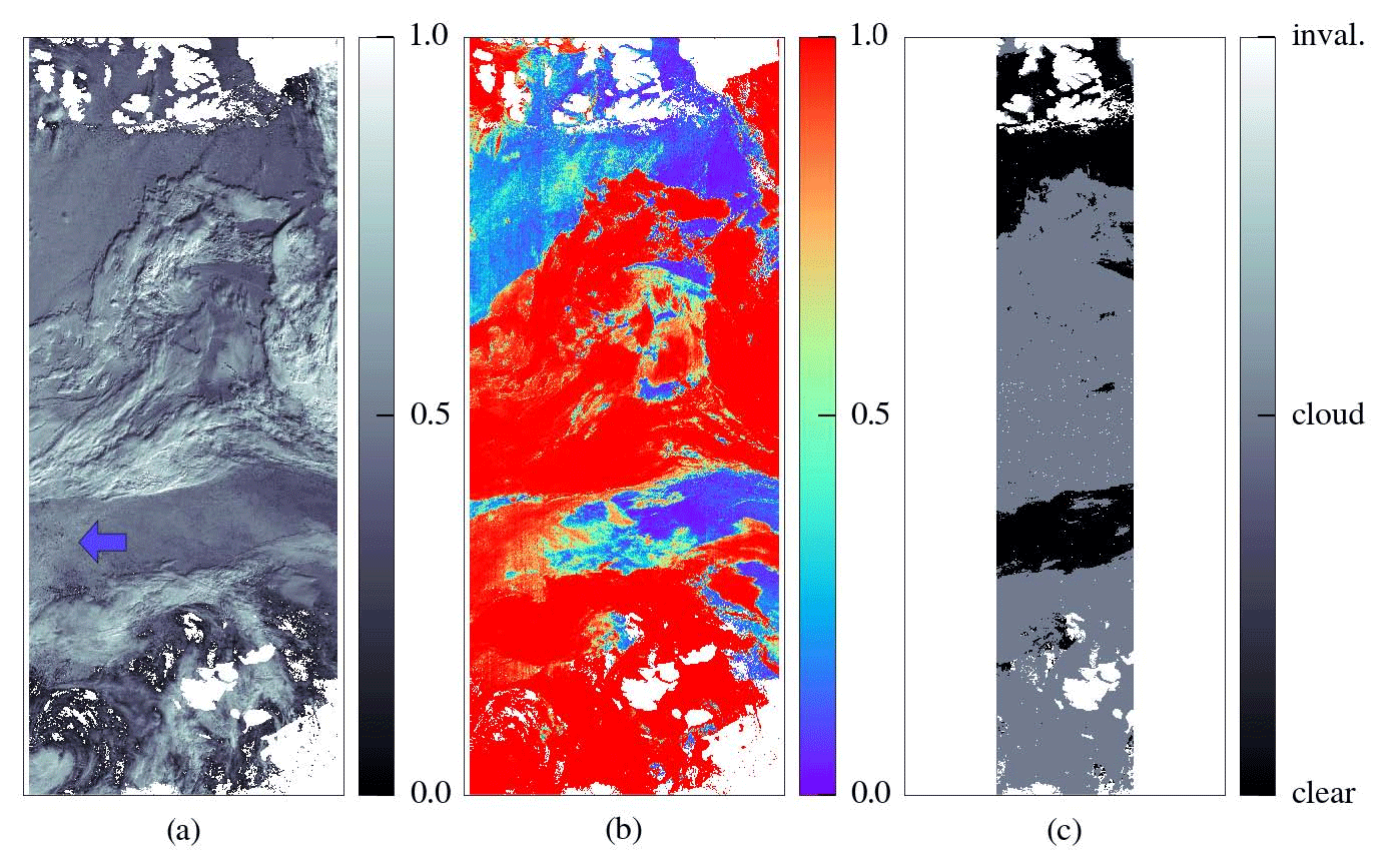
Figure 4Reflectance at 779 nm (a), cloud probability (b) and corresponding AATSR mask (c) for 31 July 2009 (orbit number 38778). The blue arrow marks a region with wrongly screened-out clear-sky pixels, although a thin cloud cover is possible.
To quantify the performance of the algorithm, we study the distribution of cloud probability for clear-sky and cloud-covered pixels in the AATSR mask (Fig. 5). For cloud-covered pixels, we find that nearly 85 % percent show a cloud probability greater than the background probability P(C)=0.86, and the distribution drops sharply towards smaller cloud probabilities (Fig. 5a). Visual inspection shows that probabilities smaller than P(C) are almost always correlated to semitransparent cloud over snow-covered ice or optically thin clouds. The distribution for clear-sky pixels is less distinct (Fig. 5b). It drops towards higher cloud probabilities, which is expected, but 6 % show a cloud probability higher than P(C) and cannot be reliably discriminated from clouds. The majority of these 6 % are the challenging case of bright, snow-covered sea ice during the beginning of the melt season and fresh snow during fall freeze-up; hence such incorrectly high cloud probability is rarely found for darker ice with melt ponds on top. Most of these false positives are connected to cloud-like values of the MDSI feature Fsi, which may potentially occur for fresh snow with fine grains. The extremely high albedo of such a surface will compromise the rox feature and prevent correct detection.
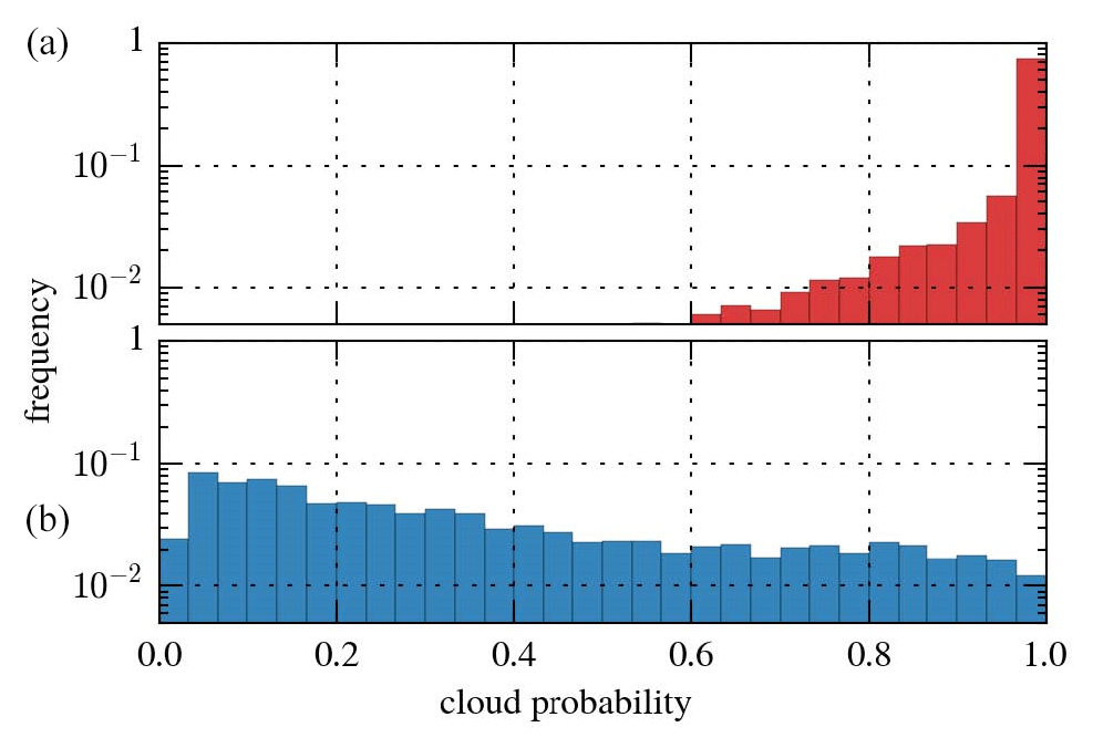
Figure 5Distribution of MECOSI cloud probability for AATSR cloud pixels (a) and AATSR clear-sky pixels (b) for May to September 2009.
We compare the MECOSI binary mask to the AATSR reference mask to study the temporal behavior of the algorithm's performance and to investigate the accuracy of the binary mask. By comparing all swaths from May to September 2009, we find that, with reference to the AATSR cloud mask, 92.51 % of the MERIS pixels are classified correctly and the remaining 7.49 % split up into 4.64 % missed cloud and 2.85 % missed clear-sky pixels. The temporal behavior of the detection rates is presented in Fig. 6. The algorithm works best in July, with detections rates around 0.9 for both clear-sky and cloud pixels, and the performance is only slightly worse in June. However, we find a considerably worse detection rate for clear-sky regions in May, August and September with values close to 0.6 and below. This indicates that more than 40 % of the pixels marked as clear sky in the AATSR mask are falsely screened out in the MECOSI binary mask. The detection rate for cloud steadily increases during June and July up to almost 1.0 at the end of the melt season. This increase is due to the state of ice surface, which gets darker over time and makes the detection of semitransparent cloud easier.
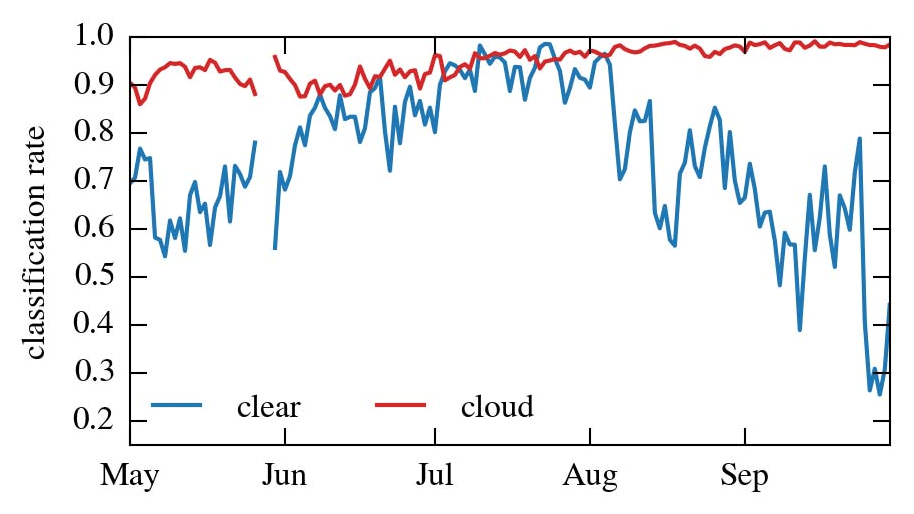
Figure 6Time series of daily mean classification rates for 2009. As an example, a value of 0.9 for cloud means that 90 % of the cloud pixels in the AATSR mask are correctly classified as cloud-covered and the remaining 10 % are missed clouds.
The binary cloud mask derived from MECOSI cloud probability is compared to the independent AATSR mask from two other years. By comparing over 3.8 × 109 pixels from 2010 and 2011, we find that 90.50 % (90.65 % for 2011) of the pixels are correctly classified, which is about 2 % less than for 2009. Thereby 5.85 % (5.92 %) are missed cloud and 3.64 % (3.42 %) are wrongly screened-out clear-sky pixels.
4.3 Extension beyond AATSR swath and comparison to MODIS cloud fraction
The accuracy of the MECOSI algorithm outside of the center half of the swath is difficult to assess because of the lack of appropriate reference data. Visual inspection of MERIS images from 2009 to 2011, which have been superimposed with the binary cloud mask, gives the general impression that the accuracy is considerably good throughout the full swath. The several cases of semitransparent clouds in May and early June 2010 are more frequently missed in the upper right quarter of the swath. The reason for this is somewhat small values in the corrected oxygen A ratio; a tendency towards smaller values on the right side of the swath is also observable in May 2009 (Fig. 2). The along-track mean of cloud probability for the year 2010 also gives slightly smaller values at the right side of the swath, as Fig. 7 shows, and the standard deviation σ increases. However, the differences across the swath are small (± 0.017 for the mean and ± 0.02 for σ) and are mainly linked to different characteristics of the five detectors of MERIS, as the jumps at the transitions and the linear behavior for the center detectors show.
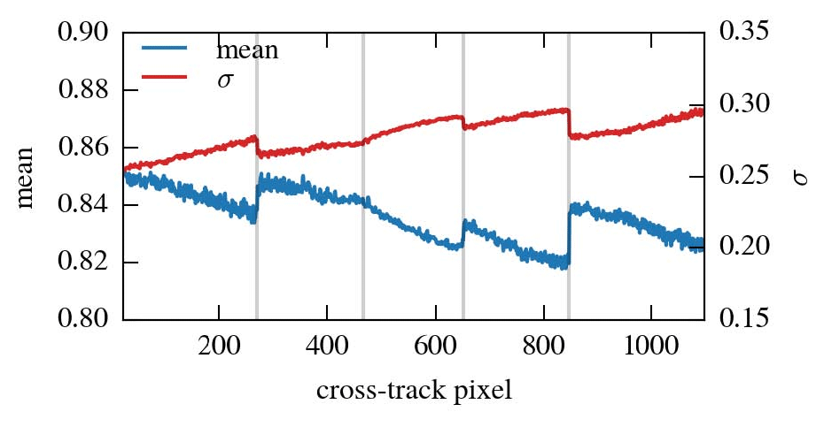
Figure 7Along-track mean and standard deviation of cloud probability for 2010. Vertical lines mark the transition between the five detectors of MERIS.
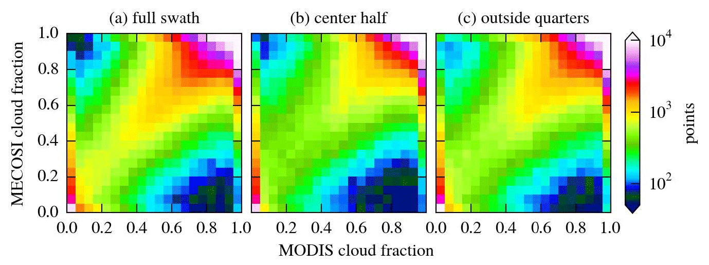
Figure 8Comparison of daily gridded MECOSI and MODIS cloud fraction using the full MERIS swath (a), the center half (b) or the outside quarters (c) for the gridded MECOSI fraction. Period is May to September 2010.
To further investigate the performance outside of the AATSR swath as well as the overall accuracy, we compare MECOSI binary cloud mask, gridded to a 1∘ constant angle grid, to MODIS cloud fraction (Ackermann et al., 2008) data from May to September 2010. Thereby, we use either the full MERIS swath, center half or the outside quarters (Fig. 8a, b and c, respectively). We find a good agreement with the MODIS data in all three cases. If the full MERIS swath is used (Fig. 8a), the comparison of over 6.7 × 10⁵ grid cells gives a root-mean-square deviation RMSD = 0.18 and a difference of means D = −0.02, which indicates that the MECOSI algorithm tends to retrieve slightly higher cloud fraction. The numbers for the central part of the swath (Fig. 8b) are very similar, with RMSD = 0.19 and D = −0.03, but the number of grid cells N = 5.0 × 10⁵ is smaller because of the restricted spatial coverage. For the outside quarters, we find again almost equal parameters with RMSD = 0.19, D = −0.01 and N = 4.6 × 10⁵, although a slight pixel displacement is seen (compare top left and bottom right corner of Fig. 8b and c).
4.4 Influence on the melt pond fraction retrieval
Finally, we study the influence of different cloud-masking schemes on the retrieved MPF. Figure 9 shows an example of using the original cloud screening built into the MPD algorithm (Zege et al., 2015; Istomina, 2017), as well as the effect of additionally applying the MECOSI and AATSR cloud masks. It is evident that both the MECOSI and the AATSR cloud mask (Fig. 9b and c) are much more restrictive than the MPD cloud masking scheme (Fig. 9a). The spatial coverage is significantly reduced and regions which are not screened out correspond well to a MODIS cloud fraction below 50 % (Fig. 9d). Differences between using the MECOSI and the AATSR cloud mask are mostly due to the limited spatial coverage of AATSR (e.g., the larger pole hole).
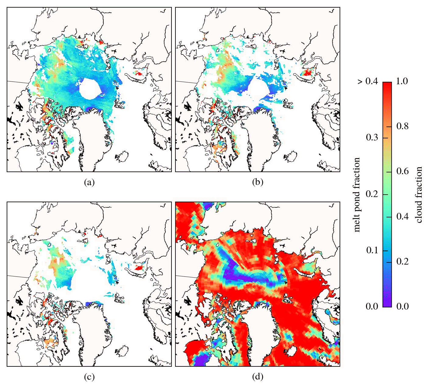
Figure 9Gridded melt pond fraction with MPD cloud mask (a), MECOSI cloud mask (b), AATSR cloud mask (c) and MODIS daytime mean cloud fraction (d), 20 June 2009.
A time series of the Arctic-wide mean MPF for all three cloud masking schemes is presented in Fig. 10. The spatial coverage has been restricted to the area seen by AATSR.
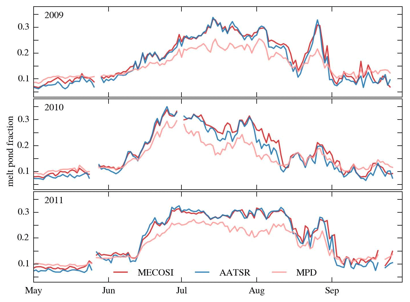
Figure 10Influence of different cloud mask on Arctic-wide mean melt pond fraction for 2009–2011. The means are calculated from gridded melt pond fraction data and coverage is restricted to the area seen by AATSR. Days with less than 100 grid cells to compare or missing AATSR data are excluded.
For all three years 2009 to 2011, we find evident differences between the original MPD product and the two improved products with additional cloud masking. The most prominent one is the significantly higher (up to 0.08 increase) mean MPF in July when additional cloud screening is applied. In May and September, however, the additional screening results in slightly smaller mean MPF. This behavior is expected because the MPD algorithm retrieves values of around 0.15 MPF for opaque clouds, so that immense cloud contamination in the original MPD product reduces the MPF value range of the time series towards this wrong MPF value.
If we focus on the differences between AATSR and MECOSI cloud mask (dark red and blue in Fig. 10), we find that both masks lead to a similar MPF time series. Using the MECOSI mask results in slightly higher MPF in May, which is possibly caused by some omitted clouds. The main advantage of the MECOSI cloud mask over AATSR is the larger spatial coverage of the latter (compare Fig. 9b and c).
The results show that the MECOSI algorithm discriminates clouds from summer sea ice with good accuracy. With MECOSI, over 90 % of the pixels are classified correctly, when compared to the AATSR reference.
Comparison to the independent MODIS daily cloud fractions shows good agreement with the developed MECOSI mask both in the center part of the MERIS swath where AATSR data are available for training and on the outside edge of the swath (Fig. 8). There is no evidence that the quality of the algorithm performance worsens towards the edges of the swath. The variation in mean cloud probability and its standard deviation across the swath are dominated by detector-to-detector differences and show no change towards the edges of the swath (Fig. 7). Therefore, we conclude that the results of the comparison to the AATSR cloud mask are, in general, valid for the full MERIS swath.
The quality of the MECOSI cloud mask for both clear and cloudy cases is the best in June and July, when the rapid melt onset and first pond drainage events happen on the Arctic sea ice (Fig. 6). Bright fresh snow compromises MECOSI cloud screening and leads to some false detections in May. The oxygen A ratio is well suited for improving the detection over fresh snow. The proposed correction scheme equalizes the ratio reasonably well (compare Fig. 1b and c). However, the detector-to-detector artifacts indicate some residual influences of the spectral smile effect, surface albedo and instrument stray light which were also not fully removed by the proposed correction scheme.
The cloud detection rates at the end of the melting season in August–September are close to 100 %. The not-as-good detection of clear cases might be connected to the reduced number of such scenes at the end of the melting season, as humidity and cloudiness increase and the ice cover decreases with the minimum ice extent, typically in the first weeks of September. For our specific application, i.e., retrieving surface parameters, it is important to screen out possibly all clouds as they bias the retrieval result. Wrong detections of clear cases as cloudy are less critical as this just reduces the spatial coverage of the product but does not affect the retrieved values.
Consequently, the MECOSI cloud screening improves the quality of the MPD MPF and albedo product. By reducing the amount of cloud contamination, we find consistently higher pond fraction in the period from mid-June to mid-August for all 3 years (Fig. 10). The cloud-contaminated pixels are no longer used as input into the MPD retrieval, and the resulting MPF dataset contains unbiased MPF and albedo values. The thus improved resulting dataset can be used for further applications, such as assimilation into or validation of climate and melt pond models.
In this work, we present MECOSI, a new cloud-screening routine for MERIS specifically developed for use over Arctic summer sea ice. Comparison to the independent MODIS cloud mask shows that the available summer Arctic MPF and spectral sea ice albedo product from MERIS (Zege et al., 2015; Istomina et al., 2015) are significantly cloud-contaminated (compare Fig. 9a and d). The cloud-screening method presented here has been developed to improve the quality of the MPF and albedo datasets.
The developed cloud-masking routine utilizes all 15 MERIS channels and a reference AATSR cloud mask to calculate probabilities of cloudy and clear cases for a given set of features:
-
oxygen A absorption and reference ratio (additionally corrected for smile effect),
-
MERIS normalized difference snow index,
-
brightness and whiteness criteria.
The dependencies on the illumination–observation geometry and the position of the pixel in the array of detectors, i.e., the detector index, have been accounted for as well. To calculate the cloudy and clear probabilities, a dataset of every AATSR and MERIS swath from 1 May to 30 September 2009 have been used to ensure a representative sample of the sea ice, snow and cloud conditions.
The developed cloud mask shows a considerable improvement over the old MPD cloud mask. The quality of cloud detection of the new algorithm is close to the reference AATSR cloud mask, whereas MERIS does not have the infrared channels which aid in the snow–cloud discrimination. The MECOSI cloud detection quality also remains high near the edges of the MERIS swath where no AATSR training data were available. Comparison to the reference AATSR and independent MODIS cloud masks shows that the application of MECOSI has greatly increased the quality of the MPD products on both spatial (Fig. 9) and temporal (Fig. 10) scales.
The advantage of MECOSI over, for example, MODIS daily cloud fraction product is that it enables accurate cloud screening of swath MERIS data over snow and sea ice, which was not possible with the old version of the cloud screening used in the MPD retrieval. The developed cloud-screening routine can be applied to remote sensing data of sea ice surfaces in both cold and melting conditions.
The developed cloud mask for MERIS over the summer Arctic sea ice, as well as the improved datasets of the melt pond fraction and spectral albedo for the entire MERIS operation time are available at the server of the University of Bremen (https://www.seaice.uni-bremen.de/start/; Istomina et al., 2017).
The developed MECOSI cloud mask for MERIS over the summer Arctic sea ice, as well as the improved datasets of the melt pond fraction and spectral albedo are available at https://www.seaice.uni-bremen.de/start/ (Istomina et al., 2017). The original MPD MPFs are available at https://seaice.uni-bremen.de/data/meris/gridded/ (Istomina, 2017).
LI conceived of the original idea and provided its first implementation, worked with the MERIS and AATSR data to prepare the training and validation of the algorithm, provided the MERIS MPF datasets, analyzed and interpreted the results, and outlined and wrote the manuscript with contributions from all authors. HM advanced the method and defined the optimal set of Bayesian features as well as performed the training and validation of the algorithm with MODIS data. MH contributed to the concept and implementation of the smile correction and the Bayesian method and contributed to the discussions. GH and GS supervised the project and aided the development of the algorithm and the discussion of the results. All authors provided critical feedback on the manuscript.
The authors declare that they have no conflict of interest.
The authors express gratitude to ESA and NASA for providing MERIS, AATSR and MODIS operational and higher-level products and to Brockmann Consult for providing the open-source software packages BEAM and SNAP.
The authors are grateful to the anonymous reviewers and the editor for their effort and valuable comments on the manuscript.
This research has been supported by the EU project SPICES (grant no. 640161) and by the Deutsche Forschungsgemeinschaft (SPP 1158
project REASSESS, grant no. 424326801).
The article processing charges for this open-access publication were covered by the University of Bremen.
This paper was edited by Alexander Kokhanovsky and reviewed by two anonymous referees.
Ackerman, S. A., Strabala, K. I., Menzel, W. P., Frey, R. A., Moeller, C. C., and Gumley, L. E.: Discriminating clear sky from clouds with MODIS, J. Geophys. Res., 103, 32141–32157, 1998.
Ackerman, S. A., Holz, R., Frey, R., Eloranta, E., Maddux, B., and McGill, M.: Cloud Detection with MODIS. Part II: Validation, J. Atmos. Ocean. Tech., 25, 1073–1086, https://doi.org/10.1175/2007JTECHA1053.1, 2008.
Allen, R. C., Durkee, P. A., and Wash, C. H.: Snow/Cloud Discrimination with Multispectral Satellite Measurements, J. Appl. Meteorol., 29, 994–1004, 1990.
Bourg, L., D'Alba, L., and Colagrande, P.: MERIS Smile Effect Characterization and Correction, Tech. rep., European Space Agency, available at: https://earth.esa.int/documents/700255/707220/MERIS_Smile_Effect.pdf (last access: 30 July 2020), 2008.
Bréon, F.-M. and Colzy, S.: Cloud detection from the spaceborne POLDER instrument and validation against surface synoptic observations, J. Appl. Meteorol., 38, 777–785, 1999.
Curry, J. A., Rossow, W. B., Randall, D., and Schramm, J. L.: Overview of Arctic cloud and radiation characteristics, J. Climate, 9, 1731–1764, https://doi.org/10.1175/1520-0442(1996)009<1731:OOACAR>2.0.CO;2, 1996.
Diner, D., Clothiaux, E., and Di Girolamo, L.: MISR Multi-angle imaging spectro-radiometer algorithm theoretical basis. Level 1 Cloud detection, Jet Propulsion Laboratory, California Institute of Technology, Pasadena, USA, JPL D-13397, 1999.
Gafurov, A. and Bárdossy, A.: Cloud removal methodology from MODIS snow cover product, Hydrol. Earth Syst. Sci., 13, 1361–1373, https://doi.org/10.5194/hess-13-1361-2009, 2009.
Gómez-Chova, L., Camps-Valls, G., Calpe-Maravilla, J., Guanter, L., and Moreno, J.: Cloud-Screening Algorithm for ENVISAT/MERIS Multispectral Images, IEEE T. Geosci. Remote, 45, 4105–4118, https://doi.org/10.1109/TGRS.2007.905312, 2007.
Hollstein, A., Fischer, J., Carbajal Henken, C., and Preusker, R.: Bayesian cloud detection for MERIS, AATSR, and their combination, Atmos. Meas. Tech., 8, 1757–1771, https://doi.org/10.5194/amt-8-1757-2015, 2015.
Istomina, L.: The MPD MPF dataset, available at: https://seaice.uni-bremen.de/data/meris/gridded/ (last access: 30 July 2020), 2017.
Istomina, L. G., von Hoyningen-Huene, W., Kokhanovsky, A. A., and Burrows, J. P.: The detection of cloud-free snow-covered areas using AATSR measurements, Atmos. Meas. Tech., 3, 1005–1017, https://doi.org/10.5194/amt-3-1005-2010, 2010.
Istomina, L. G., von Hoyningen-Huene, W., Kokhanovsky, A. A., Schultz, E., and Burrows, J. P.: Remote sensing of aerosols over snow using infrared AATSR observations, Atmos. Meas. Tech., 4, 1133–1145, https://doi.org/10.5194/amt-4-1133-2011, 2011.
Istomina, L., Nicolaus, M., Perovich, D. K.: Spectral albedo of sea ice and melt ponds measured during POLARSTERN cruise ARK-XXVII/3 (IceArc) in 2012, Institut für Umweltphysik, Universität Bremen, PANGAEA, https://doi.org/10.1594/PANGAEA.815111, 2013.
Istomina, L., Heygster, G., Huntemann, M., Schwarz, P., Birnbaum, G., Scharien, R., Polashenski, C., Perovich, D., Zege, E., Malinka, A., Prikhach, A., and Katsev, I.: Melt pond fraction and spectral sea ice albedo retrieval from MERIS data – Part 1: Validation against in situ, aerial, and ship cruise data, The Cryosphere, 9, 1551–1566, https://doi.org/10.5194/tc-9-1551-2015, 2015.
Istomina, L., Marks, H., and Huntemann, M.: MECOSI cloud screening dataset, University of Bremen, available at: https://www.seaice.uni-bremen.de/start/ (last access: 30 July 2020), 2017.
Jäger, M.: Advanced MERIS Channel 11 Smile Correction as a Basis for Cloud Top Height Estimation Developed from SCIATRAN Radiative Transfer Calculations in the O2-A Absorption Band, Master's thesis, University of Bremen, Bremen, Germany, 2013.
Kalnay, E., Kanamitsu, M., Kistler, R., Collins, W., Deaven, D., Gandin, L., Iredell, M., Saha, S., White, G., Woollen, J., Zhu, Y., Leetmaa, A., Reynolds, B., Chelliah, M., Ebisuzaki, W., Higgins, W., Janowiak, J., Mo, K. C., Ropelewski, C., Wang, J., Jenne, R., and Joseph, D.: The NCEP/NCAR 40-year reanalysis project, B. Am. Meteorol. Soc., 77, 437–470, https://doi.org/10.1175/1520-0477(1996)077<0437:TNYRP>2.0.CO;2, 1996.
Key, J. and Barry, R.G.: Cloud cover analysis with Arctic AVHRR data. 1. Cloud detection, J. Geophys. Res., 94, 18521–18535, 1989.
Kokhanovsky, A. A.: Cloud Optics, edited by: Mysak, L. A. and Hamilton, K., Springer, Dordrecht, the Netherlands, 2006.
Kokhanovsky, A. A., von Hoyningen-Huene, W., and Burrows, J. P.: Determination of the cloud fraction in the SCIAMACHY ground scene using MERIS spectral measurements, Int. J. Remote Sens., 30, 6151–6167, https://doi.org/10.1080/01431160902842326, 2009.
Krijger, J. M., Tol, P., Istomina, L. G., Schlundt, C., Schrijver, H., and Aben, I.: Improved identification of clouds and ice/snow covered surfaces in SCIAMACHY observations, Atmos. Meas. Tech., 4, 2213–2224, https://doi.org/10.5194/amt-4-2213-2011, 2011.
Lindstrot, R., Preusker, R., and Fischer, J.: Empirical Correction of Stray Light within the MERIS Oxygen A-Band Channel, J. Atmos. Ocean. Tech., 27, 1185–1194, https://doi.org/10.1175/2010JTECHA1430.1, 2010.
Liu, Y., Key, J. R., Frey, R. A., Ackerman, S .A., and Menzel, W. P.: Nighttime polar cloud detection with MODIS, Remote Sens. Environ., 92, 181–194, 2004.
Lotz, W. A., Vountas, M., Dinter, T., and Burrows, J. P.: Cloud and surface classification using SCIAMACHY polarization measurement devices, Atmos. Chem. Phys., 9, 1279–1288, https://doi.org/10.5194/acp-9-1279-2009, 2009.
Lyapustin, A. and Wang, Y.: The time series technique for aerosol retrievals over land from MODIS, Satellite Aerosol Remote Sensing over Land, edited by: Kokhanovsky A. A. and de Leeuw, G., Springer Praxis Publ., Chichester, UK, 69–99, 2009.
Lyapustin, A., Wang, Y., and Frey, R.: An automated cloud mask algorithm based on time series of MODIS measurements, J. Geophys. Res., 113, D16207, https://doi.org/10.1029/2007JD009641, 2008.
Madhavan, S., Angal, A., Dodd, J., Sun, J., and Xiong, X.: Analog and digital saturation in the MODIS reflective solar bands, Proc. SPIE 8510, Earth Observing Systems XVII, 85101N, https://doi.org/10.1117/12.929998, 2012.
Marks, H.: Investigation of Algorithms to Retrieve Melt Pond Fraction on Arctic Sea Ice from Optical Satellite Observations, Master's thesis, Universität Tübingen, Tübingen, Germany, 2015.
Martins, J. V., Tanré, D., Remer, L., Kaufman, Y., Mattoo, S., and Levy, R.: MODIS Cloud screening for remote sensing of aerosols over oceans using spatial variability, Geophys. Res. Lett., 29, 8009, https://doi.org/10.1029/2001GL013252, 2002.
Minnis, P., Chakrapani, V., Doelling, D. R., Nguyen, L., Palikonda, R., Spangenberg, D. A., Uttal, T., Arduini, R. F., and Shupe, M.: Cloud coverage and height during FIRE ACE derived from AVHRR data, J. Geophys. Res., 106, 15215–15232, 2001.
Nicolaus, M., Katlein, C., Maslanik, J., and Hendricks, S.: Changes in Arctic sea ice result in increasing light transmittance and absorption: LIGHT IN A CHANGING ARCTIC OCEAN, Geophys. Res. Lett., 39, L24501, https://doi.org/10.1029/2012GL053738, 2012.
Preusker, R. and Lindstrot, R.: Remote Sensing of Cloud-Top Pressure Using Moderately Resolved Measurements within the Oxygen A Band – A Sensitivity Study, J. Appl. Meteorol. Clim., 48, 1562–1574, https://doi.org/10.1175/2009JAMC2074.1, 2009.
Schlundt, C., Kokhanovsky, A. A., von Hoyningen-Huene, W., Dinter, T., Istomina, L., and Burrows, J. P.: Synergetic cloud fraction determination for SCIAMACHY using MERIS, Atmos. Meas. Tech., 4, 319–337, https://doi.org/10.5194/amt-4-319-2011, 2011.
Schröder, D., Feltham, D., Flocco, D., and Tsamados, M.: September Arctic sea-ice minimum predicted by spring melt-pond fraction, Nat. Clim. Change 4, 353–357, https://doi.org/10.1038/NCLIMATE2203, 2014.
Spangenberg, D. A., Chakrapani, V., Doelling, D. R., Minnis, P., and Arduini, R. F.: Development of an automated Arctic cloud mask using clear-sky satellite observations taken over the SHEBA and ARM NSA sites, Proc. 6th Conf. on Polar Meteor., and Oceanography, 14–18 May 2001, San Diego, CA, USA, 246–249, 2001.
Trepte, Q., Arduini, R. F., Chen, Y., Sun-Mack, S., Minnis, P., Spangenberg, D. A., and Doelling, D. R.: Development of a daytime polar cloud mask using theoretical models of near-infrared bidirectional reflectance for ARM and CERES, Proc. AMS 6th Conf. Polar Meteorology and Oceanography, San Diego, CA, USA, 4–18 May 2001, 242–245, 2001.
Warren, S. G.: Optical Properties of Snow, Rev. Geophys., 20, 67–89, 1982.
Wiebe, H., Heygster, G., Zege, E., Aoki, T., and Hori, M.: Snow grain size retrieval SGSP from optical satellite data: Validation with ground measurements and detection of snow fall events, Remote Sens. Environ., 128, 11–20, https://doi.org/10.1016/j.rse.2012.09.007, 2013.
Zege, E., Malinka, A., Katsev, I., Prikhach, A., Heygster, G., Istomina, L., Birnbaum, G., and Schwarz, P.: Algorithm to retrieve the melt pond fraction and the spectral albedo of Arctic summer ice from satellite optical data, Remote Sens. Environ., 163, 153–164, https://doi.org/10.1016/j.rse.2015.03.012, 2015.