the Creative Commons Attribution 4.0 License.
the Creative Commons Attribution 4.0 License.
 | 04 Dec 2020
Atmospheric observations with E-band microwave links – challenges and opportunities
Michal Dohnal
Pavel Valtr
Martin Grabner
Vojtěch Bareš
Opportunistic sensing of rainfall and water vapor using commercial microwave links operated within cellular networks was conceived more than a decade ago. It has since been further investigated in numerous studies, predominantly concentrating on the frequency region of 15–40 GHz. This article provides the first evaluation of rainfall and water vapor sensing with microwave links operating at E-band frequencies (specifically 71–76 and 81–86 GHz). These microwave links are increasingly being updated (and are frequently replacing) older communication infrastructure. Attenuation–rainfall relations are investigated theoretically on drop size distribution data. Furthermore, quantitative rainfall estimates from six microwave links, operated within cellular backhaul, are compared with observed rainfall intensities. Finally, the capability to detect water vapor is demonstrated on the longest microwave link measuring 4.86 km in path length. The results show that E-band microwave links are markedly more sensitive to rainfall than devices operating in the 15–40 GHz range and can observe even light rainfalls, a feat practically impossible to achieve previously. The E-band links are, however, substantially more affected by errors related to variable drop size distribution. Water vapor retrieval might be possible from long E-band microwave links; nevertheless, the efficient separation of gaseous attenuation from other signal losses will be challenging in practice.
- Article
(7418 KB) - Full-text XML
-
Supplement
(256 KB) - BibTeX
- EndNote


Electromagnetic (EM) waves in the microwave region are attenuated by water vapor, oxygen, fog, or raindrops. Measurements of microwave attenuation at different frequency bands thus represent an invaluable source of information regarding the atmosphere. Passive and active microwave systems have become an integral part of Earth-observing satellites, terrestrial remote sensing systems, and complete remote sensing methods in other spectral regions (Woodhouse, 2017). The microwave region is, however, also increasingly utilized in communication systems, allowing for new possibilities to observe the atmosphere with unintentional (opportunistic) sensing. Commercial microwave links (CMLs) are an excellent example of a communication system capable of providing close-to-ground observations of the atmosphere. CMLs are point-to-point line-of-sight radio connections widely used in mobile phone backhaul for connecting hops of different lengths, typically ranging from tens of meters to several kilometers. About 4 million CMLs were operated worldwide within cellular backhaul in 2016 (Ericsson, 2016) and about 5 million in 2018 (Ericsson, 2018). Most of these CMLs are operated at frequencies between 15 and 40 GHz (Ericsson, 2016, 2018), where raindrops and, to a lesser extent, water vapor represent a significant source of attenuation (Atlas and Ulbrich, 1977; Liebe et al., 1993). Information on the attenuation of any CML within countrywide networks is practically accessible in real time with a delay of several seconds from a remote location, typically a network operation center (Chwala et al., 2016) creating an appealing opportunistic sensing system capable of providing close-to-ground observations of rainfall intensity (Leijnse et al., 2007; Messer et al., 2006) and water vapor density (David et al., 2009).
CML rainfall retrieval methods developed over the last decade have been predominantly designed and tested for frequency bands between 15 and 40 GHz (Chwala and Kunstmann, 2019). Attenuation caused by raindrops is, in this frequency region, almost linearly related to rainfall intensity and does not strongly depend on drop size distribution (DSD) (Berne and Uijlenhoet, 2007). Water vapor retrieval has been proposed for CMLs operating around 22 GHz (David et al., 2009), where there is a resonance line of water vapor. Increasing demands on data transfer force operators to utilize higher-frequency spectra, and a new generation of E-band CMLs, operating at the 71–86 GHz frequency band, is gradually modernizing cellular backhaul networks, especially in cities, where they often replace older devices. The share of E-band CMLs in mobile phone backhaul has already reached 20 %, e.g., in Poland and the Czech Republic, and it is expected to grow in other countries as E-band CMLs are considered an essential part of new 5G networks (Ericsson, 2019).
E-band CMLs should be, according to recommendations for designing CMLs (ITU-R, 2005), more sensitive to rainfall; nevertheless, the relation between rainfall intensity and attenuation is not linear. Furthermore, E-band radio waves have 2 to 4 times shorter wavelengths, and the extinction efficiency is highest for smaller raindrops. Thus, the attenuation–rainfall relation is more sensitive to drop size distribution, which has been already demonstrated in several propagation experiments, e.g., by Hansryd et al. (2010) or Luini et al. (2018). Radio-wave propagation at an E-band is also more sensitive to water vapor, which poses a challenge when separating rainfall-induced attenuation from other sources of attenuation. On the other hand, the sensitivity to water vapor might also enable its detection or even monitoring.
This article provides the first evaluation of E-band CMLs as rainfall and water vapor sensors. The capabilities of E-band CMLs for weather monitoring are theoretically evaluated and demonstrated on attenuation data retrieved between August and December 2018 from six E-band CMLs operated within cellular backhaul of a commercial provider in Prague (T-Mobile Czech Republic). The ultimate goal of this investigation is to provide an overview of the challenges and opportunities related to atmospheric observations with E-band CMLs. Section 2 of the article summarizes, based upon previous works, the principles behind retrieving atmospheric variables from CML observations. Section 3 describes the methodology and datasets used in this article for the assessment of E-band CMLs; in addition, analysis estimating wet antenna attenuation and analysis evaluating the effect of DSD on the attenuation–rainfall relation are presented. Section 4 presents the results of the case study. The results are further interpreted and discussed in Sect. 5, followed by the conclusions presented in Sect. 6.
2.1 Components of total observed loss
Standard CMLs are monitored for transmitted tx (dBm) and received rx (dBm) signal power and the difference between tx and rx is the total observed loss Lt (dB), which can be separated into several components:
where Lbf (dB) is free space loss; Lm (dB) represents losses in the medium; Ltc (dB) and Lrc (dB) are losses at the transmitting and receiving antennas, respectively; and Gt (dB) and Gr (dB) are antenna directive gains (Internationale Fernmelde-Union, 2009). Free space loss, Lbf, is uniquely defined by the distance d (m) between the transmitter and receiver and by wavelength λ (m):
The sum of antenna losses and gains is given by their hardware. It includes interference with the environment close to antennas as antenna loss can change, e.g., due to the wetness of antenna radomes. The propagation mechanisms influencing loss in the medium, Lm, consist of attenuation due to atmospheric gases, including water vapor, which is usually not exceeding 1.5 dB km−1 (Sect. 2.2); attenuation due to precipitation, which can reach several tens of decibels per kilometer (dB km−1) (Sect. 2.3); attenuation due to obstacles in the wave path; and diffraction losses causing bending of the direct wave towards the ground. Total loss can also be influenced by so-called multipath interference occurring due to the constructive or destructive phase summation of the signal at the receiving antenna during the atmospheric multipath propagation conditions (Valtr et al., 2011). Precise separation and quantification of different components of total loss requires a detailed description of atmospheric conditions along a CML path as well as conditions affecting the hardware of transmitting and receiving stations. The specific path attenuation due to raindrops or due to water vapor k (dB km−1) is thus usually separated from other sources of attenuation using a data-driven approach:
where l (km) is CML path length; B (dB) is background attenuation, so-called baseline; and Aw (dB) is wet antenna attenuation (WAA) caused by antenna radome wetting during rainfall or dew events. Baseline is most commonly estimated from attenuation levels during periods without rain and dew on antennas (Overeem et al., 2011; Schleiss and Berne, 2010). WAA estimation is discussed in more detail in Sect. 2.4. The accurate quantification of WAA is especially important for shorter CMLs attenuated by raindrops along a short path, by which the relative importance of the WAA contribution is significant.
We further refer to the periods with and without rain or dew occurrence as wet and dry weather, respectively. The term loss is used when referring to reduction in power density of an EM wave in decibel (dB). In contrast, the term attenuation mostly refers to specific attenuation (dB km−1) apart from WAA where it means loss (dB). We, nevertheless, stick to the term WAA as it is already established in the literature.
2.2 Attenuation by atmospheric gases
Attenuation by atmospheric gases is caused predominantly by the interaction of an EM wave with molecules of water and oxygen. The evaluation of gas attenuation, as described in ITU-R (2019) and originally in Liebe et al. (1993), is based on the concept of the complex refractive index. In a medium with complex refractive index n, the intensity of EM wave I (W m−2) is attenuated at distance x (m) as
where (m) is a vacuum wave number, f (GHz) the EM wave frequency, c (m s−1) the speed of light, and Im(n) denotes the imaginary part of n. After introducing complex refractivity , the specific attenuation k (dB km−1) is obtained as
with the EM wave frequency f expressed in gigahertz (GHz).
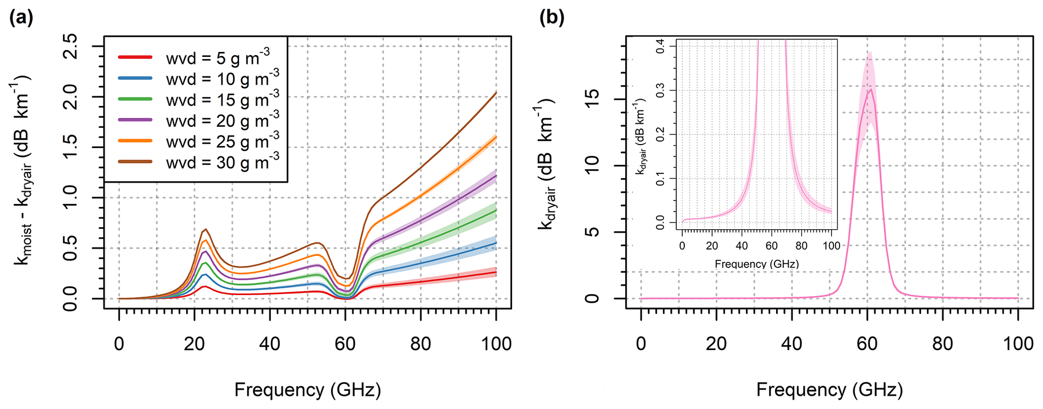
Figure 1(a) Attenuation of EM waves by water vapor for frequencies 0 to 100 GHz. The relation is shown for different water vapor densities (wvd) for temperatures −10 to +30 ∘C and pressures 1000 to 1030 hPa (colored bands). (b) Dry-air attenuation of EM waves for temperatures −10 to +30 ∘C and pressures 1000 to 1030 hPa (total spread represented by colored bands) are shown; inset: a detailed view of the lower attenuations.
In Eq. (5), the attenuation due to water vapor is defined as the difference between wet-air and dry-air attenuation under the same moist-air pressure and temperature. Thus, the effect of water vapor on dry-air attenuation is considered (ITU-R, 2019): first, dry-air pressure decreases during humid conditions (under the assumption of constant moist-air pressure), and second, partial water pressure affects the rate of collisions between the molecules (pressure broadening). Figure 1 shows specific attenuation by water vapor and dry air. Attenuation due to water vapor monotonically increases as the water vapor density increases. Water vapor density can thus be uniquely determined from gaseous attenuation when temperature and air pressure is known. David et al. (2009) suggested that CMLs operating around 22 GHz might be sufficiently sensitive to gaseous attenuation, enabling estimation of water vapor density. Recently, daily water vapor estimates from multiple CMLs operating around 22 GHz were evaluated (David et al., 2019); nonetheless, water vapor retrieval from E-band CMLs has not been reported yet. Water vapor attenuation in the E-band is about 2 times higher than around 22 GHz; however, it is also significantly more sensitive to temperature and to a lesser extent air pressure (Fig. 1a). The temperature and pressure also influence dry-air attenuation, especially at frequencies closer to 60 GHz (Fig. 1b).
2.3 Relation between raindrop path attenuation and rainfall intensity
Attenuation of a direct EM wave due to raindrops can be precisely calculated using scattering theory. Attenuation caused by a single raindrop is determined by the wavelength, refractive index of water, and shape parameters of the raindrop and its orientation. The extinction cross section Cext (cm2), which can be calculated using the T-matrix method (Mishchenko and Travis, 1998), characterizes the scattering and absorption properties of each raindrop for a given frequency and polarization. The total drop density in the unit volume Nt (m−3) is relatively small for natural rainfalls. Therefore, multiple scattering effects can be neglected. The specific raindrop path attenuation k (dB km−1) can thus be considered a sum of attenuations caused by single raindrops and can be expressed in integral form:
where D (mm) denotes the equivolumetric spherical drop diameter, and N(D) (m−3 mm−1) is the number of drops in unit volume per drop diameter interval. N(D) also determines rainfall intensity R (mm h−1):
where v(D) (m s−1) is the terminal velocity of raindrops given by their diameters. The relation between attenuation and rainfall intensity can be approximated by a power law (Olsen et al., 1978):
where a (mm−b hb dB km−1) and b (–) are empirical parameters dependent on frequency, polarization, and DSD. When estimating rainfall from observed attenuation, Eq. (8) can be reformulated to
where α (mm h−1 dB−β kmβ) = and β (–) = b−1.
Models (8) and (9) approximate the attenuation–rainfall relation well at frequencies around 30 GHz. Nonetheless, errors increase for both lower and higher frequencies due to variable DSD (Berne and Uijlenhoet, 2007). Berne and Uijlenhoet (2007), however, investigated sensitivity to DSD only for the frequency region of 5–50 GHz. A detailed evaluation of the attenuation–rainfall model for the E-band has not been reported, yet higher sensitivity of E-band CMLs to DSD has been demonstrated during several propagation experiments (Hansryd et al., 2010; Luini et al., 2018).
2.4 Wet antenna attenuation
Wet antenna attenuation (WAA) is caused by a water layer forming on antenna radomes during rainfall events or dew occurrence. WAA can be modeled using EM full-wave simulators (Mancini et al., 2019; Moroder et al., 2020) solving, numerically, Maxwell's equations; nevertheless, such simulations are computationally demanding and require characterization of water distribution (e.g., thin film, droplets, rivulets) and its volume on antenna radomes. The formation of water film on antennas is, however, a complex process dependent on rainfall intensity, wind direction and velocity, or air and rain-water temperature, as well as on antenna radome hydrophobic properties. On the other hand, WAA represents a substantial part of total loss (Fencl et al., 2019), especially by shorter CMLs, and its identification and separation from attenuation caused by raindrops along a CML path is crucial when obtaining reliable rainfall estimates.
Most of the models, suggested explicitly for microwave link rainfall retrieval, are empirical and designed for lower frequencies (Minda and Nakamura, 2005; Overeem et al., 2011; Schleiss et al., 2013). However, the semiempirical model suggested by Leijnse et al. (2008) enables WAA for an arbitrary frequency to be calculated. The Leijnse model assumes a layer of water with the constant thickness assumed to be related to rainfall intensity by a power law. The parameters of this relation need to be optimized. According to the Leijnse model, WAA typical of E-band CML frequencies is about 2 times higher than 38 GHz. Hong et al. (2017), however, showed with 72 and 84 GHz microwave links that WAA depends highly on specific hardware settings. An antenna without radome experienced WAA of about 7 dB during a spraying experiment with artificial rain. The antenna covered by a radome (a typical setting of CMLs) experienced WAA of approx. 2 dB and WAA decreased further to only approx. 0.3 dB when a radome with hydrophobic coating was used. Similarly, low values of WAA at E-band CMLs have been reported by Ostrometzky et al. (2018), who observed WAAs of 0.86 ± 0.54 and 1.07 ± 0.75 dB at two 73 GHz CMLs. These values are significantly lower than previously observed WAA at lower frequencies (Fencl et al., 2019; Minda and Nakamura, 2005; Schleiss et al., 2013), although E-band CMLs should be, in theory, more sensitive to WAA (Leijnse et al., 2008).
The E-band evaluation concentrates on (i) the separation of gaseous attenuation from total observed loss, which is a prerequisite for CML water vapor retrieval; (ii) the relation between raindrop attenuation and rainfall intensity, including the effect of DSD; and (iii) the influence of WAA on CML quantitative precipitation estimates (QPEs). The methodology combines numerical experiments using virtual attenuation time series simulated from weather observations with analyses of CML observations obtained during the dedicated case study. Datasets from two experimental sites are used for this purpose.
3.1 Experimental sites and datasets
Duebendorf data are used for analyzing the sensitivity of the attenuation–rainfall relation to drop size distribution. Drop size distribution is obtained from a PARSIVEL disdrometer (first generation, manufactured by OTT). Drop counts and fall velocities are recorded over 30 s intervals. The data were collected during the CoMMon experiment in Duebendorf (Switzerland), which is described, for example, in Wang et al. (2012). Duebendorf data span from March 2011 to April 2012.
The disdrometer data are quality checked and suspicious records are excluded using filters described in Jaffrain and Berne (2010). Moreover, only records classified by the disdrometer as rainfall (at least from 90 %) are used for further analysis; hail events are excluded. In addition, particles larger than 5.5 mm are not considered to be raindrops and thus excluded from the analysis. The data which pass the quality check are aggregated to a 1 min temporal resolution using averaging.
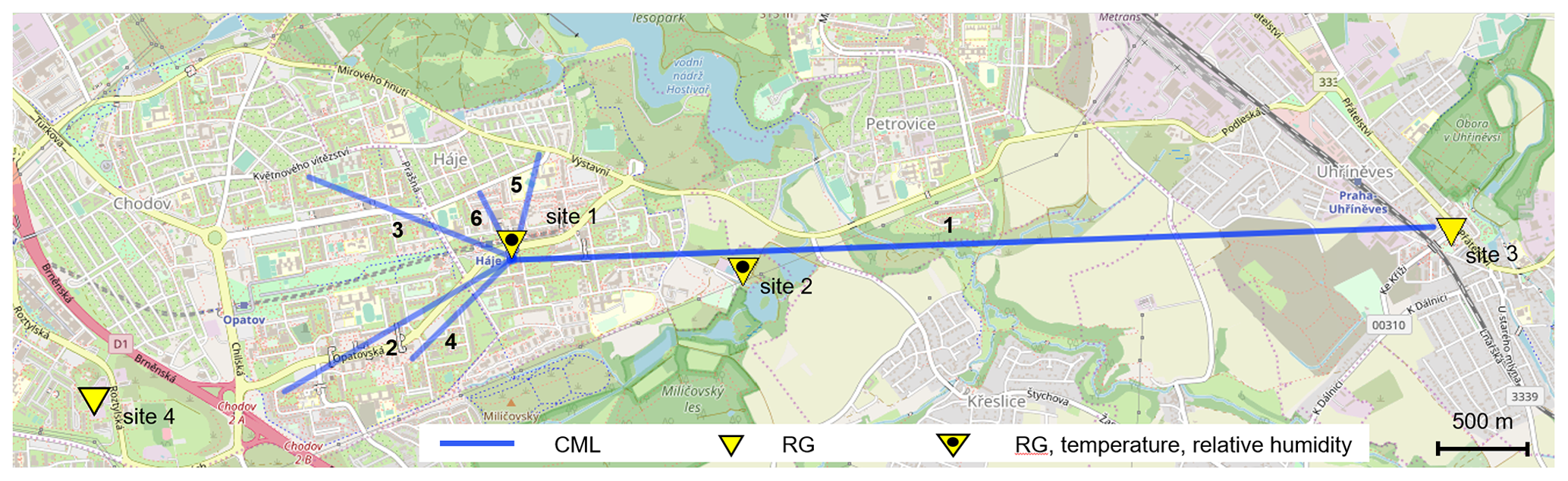
Figure 2Case study area Prague-Haje, Czech Republic. Two of the rain gauges are equipped with air humidity and temperature probes. © OpenStreetMap contributors. Distributed under a Creative Commons BY-SA License.
Prague data are used for analyzing gaseous attenuation and evaluating rainfall retrieval from E-band CMLs. The CMLs (Table 1) are located in the southeast suburb of Prague (Czech Republic). Five shorter CMLs are located in a residential area with a housing estate. The path of the long CML goes over an area with mostly agricultural land use (Fig. 2). The main node from which all CML paths originate is located on the roof of a 65 m tall building; the end nodes are about 15 to 30 m above ground. All the CMLs operate at an Ericsson MINILINK platform and were deployed to the site during 2016 and 2017. CMLs have a full-duplex configuration with two sublinks operating in one direction at 73–74 GHz and in the second direction at 83–84 GHz with a duplex separation of 10 GHz. Transmitted signal power tx and received signal power rx are collected with custom-made server-side software which polls selected CMLs using SNMP (Simple Network Management Protocol) and stores records into a PostgreSQL database. The sampling time step is approx. 10 s. The resolution of a tx and rx reading is 0.1 dBm. All devices have automatic transmitted power control (ATPC), i.e., transmitted power is automatically controlled to minimize fluctuations in rx. CML data acquisition is described in detail in the Supplement.
Table 1CML characteristics in Prague-Haje, Czech Republic. The suffixes “a” and “b” denote sublinks of a CML.

Tipping bucket rain gauges (MR3, METEOSERVIS v.o.s., catch area 500 cm2, resolution 0.1 mm) have been deployed at four measuring sites. Two rain gauges are located at the end nodes of the long CML: one at ground level close to the CML path about 1.5 km from the main network node and one about 2 km southwest from the main node. The rain gauges at sites 1 and 2 are equipped with temperature and air humidity sensors collecting observations in a 5 min time step. All four rain gauges have been regularly maintained (monthly) and are dynamically calibrated (Humphrey et al., 1997). We further refer to the case study dataset as Prague data (Fencl et al., 2020).
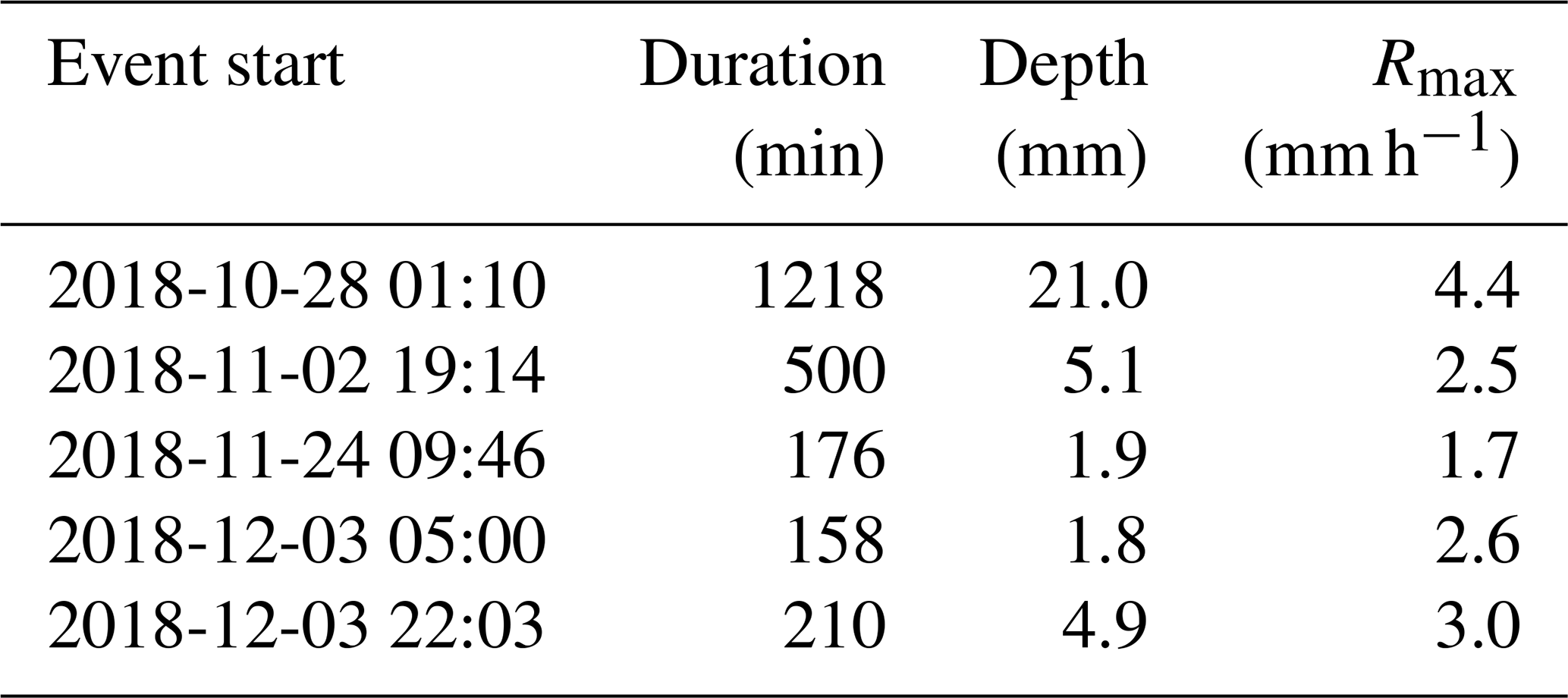
Rain-gauge data are separated into rainfall events. An event is defined as a period with intervals between consecutive rain-gauge tips shorter than 1 h. The rainfall events with rainfall depth lower than 1 mm are excluded from the evaluation. Furthermore, events during which the temperature dropped below 2 ∘C were also excluded from the evaluation to limit the performance assessment to liquid precipitation only. This results in a set of five events (see Table 2) representing, in terms of total depth, 81 % of all the precipitation during the experimental period. Rainfall data are aggregated by averaging to a 15 min temporal resolution to limit uncertainties due to rain-gauge quantization and uncertainties related to uncaptured rainfall spatial variability. The 15 min rainfall intensities are, for all four rain gauges, highly correlated (r=0.88–0.96). The cumulative rainfall observed by the rain gauges is also in excellent agreement and differs from the mean rainfall only by 1 %–3 %. The air temperature and relative humidity data (5 min temporal resolution) are not further processed. The correlation coefficient between temperature observations is 0.95 and between humidity observations is 0.86. In general, observations on the 65 m tall building (site 1) have slightly lower variability than close-to-ground observations (site 2). The discrepancies are especially pronounced during transient conditions in the morning. Prague data span from 20 August to 16 December 2018. The rainfall observations are, due to technical problems, available from 28 October to 16 December 2018.
Table 2Rainfall events used for the evaluation of CML rainfall retrieval in UTC (YYYY-mm-dd HH:MM).
3.2 CML data processing
First, total loss is calculated for each CML as the difference between transmitted and received signal powers (Eq. 1). The total loss data are aggregated using averaging to a 1 min temporal resolution.
Quality check. All the time series of total losses are visually inspected to identify noticeable hardware related artifacts. In one case (CML 2), the sudden change in the baseline is manually corrected, as automated procedures used for attenuation processing are not designed to cope with this artifact. Hardware-related artifacts are presented in more detail in Appendix B.
Baseline identification for rainfall retrieval. Background attenuation, the so-called baseline, is needed to identify rainfall-induced attenuation (Eq. 3) and is estimated as a moving median with a centered window having a size of 1 week applied on time series of total losses averaged over 15 min intervals. A 1-week window size seems to be appropriate for the climate of the Czech Republic as it covers a period with more than half of the records categorized as dry weather. On the other hand, it is sufficiently short to reliably capture long-term baseline drifts related to the instability of the CML hardware or gaseous attenuation. Although dry–wet weather classification based solely on CML observations is not used for baseline identification in this study, it is included in Appendix A as it might be needed for future studies and applications (see Discussion section).
Baseline identification for evaluating gaseous attenuation. The constant baseline is set separately for each sublink (73.5 and 83.5 GHz), such that the median attenuation obtained after the baseline separation corresponds to the median theoretical attenuation (Sect. 3.5). The median attenuation is calculated considering dry-weather periods only, i.e., periods without rainfall and dew occurrences (events causing the tipping of at least one of the rain gauges). A safety window of 6 h was set before and after each event with an event considered to start with the first tip of any rain gauge and ending with the last tip.
Wet antenna attenuation. The WAA during rainfall is modeled as constant (Overeem et al., 2011) and is set to 2.7 and 2.3 dB for all 73–74 and 83–84 GHz sublinks, respectively. The magnitudes of WAA are estimated as the median of WAA values quantified during the analysis presented in Sect. 3.4. The WAA magnitude of zero is considered during dry-weather periods.
3.3 Sensitivity of the k–R model to drop size distribution
The analysis of the k–R model (Eq. 9) with respect to DSD is based on fitting Eq. (9) on attenuation and rainfall intensities obtained from Eq. (6) and (7), respectively. The investigation is performed on PARSIVEL observations of DSD from the Duebendorf dataset. The classification of rainfalls based on their mass-weighted diameter enables us to optimize the k–R model separately for rainfall with different drop sizes.
Specific attenuations are calculated according to Eq. (6) for each DSD record. Extinction cross sections entering Eq. (6) are calculated using the T-Matrix model (Mishchenko and Travis, 1998) implemented in Python (Leinonen, 2014). The calculation assumes a temperature of 10 ∘C, canting angle of 0∘, oblate spheroid drop shape, drop axial ratio according to Pruppacher and Beard (1970), and a custom heuristic approximation of the formula by Pruppacher and Beard for drops smaller than 0.5 mm. Specific attenuations are calculated for 73.5 and 83.5 GHz (vertical polarization), i.e., frequencies of the sublinks belonging to the long CML in the Prague data. These frequencies are approximately in the middle of the frequency bands of 71–76 and 81–86 GHz allocated for E-band fixed wireless services and are thus representative for all E-band CMLs.
The rainfall records are classified into two groups according to the mass-weighted drop diameter Dm (mm), which is the ratio between the fourth and third DSD moments:
The mass-weighted diameter Dm is a common descriptor of the center of a probability density function f(D) characterizing DSD. The mass-weighted diameter can be approximately related to the rainfall intensity by a power-law function:
where R (mm h−1) is rainfall intensity and γ (mm mm−δ hδ) and δ (–) are empirical parameters. The approximation (Eq. 11) is used to calculate a classification threshold dependent on rainfall intensity. Parameters γ and δ are estimated by fitting Eq. (11) to Dm as derived from PARSIVEL records using Eq. (10). Specifically, the sum of squared residuals between Dm obtained from Eqs. (10) and (11) is minimized. This results in parameters γ=1.29 mm mm−δ hδ and δ=0.16. The Dm-based classification separates rainfalls by the size of their raindrops into two classes and roughly evaluates the convective and stratiform nature of the precipitation in the Duebendorf dataset (Jaffrain and Berne, 2012). We further refer to those two classes as “stratiform” and “convective”. Records with Dm larger than or equal to capped Dm (Eq. 11) are classified as convective and time steps with Dm smaller than capped Dm are classified as stratiform.
The k–R model (Eq. 9) is fitted separately for each frequency and rainfall type by minimizing the sum of squared residuals between reference rainfall intensities (Eq. 7) and rainfall intensities estimated by the model using a specific attenuation obtained by Eq. (6). In addition, the k–R model is also fitted for all the records together.

Figure 3Relation between specific attenuation and rainfall derived from 1 year of DSD data for vertically polarized EM waves at frequencies (a) 73.5 GHz and (b) 83.5 GHz. Parameters of the k–R models (Eq. 9) are shown. Insets show in detail the attenuation–rainfall relation and the k–R models for low specific attenuations and light rainfalls.
The relation between rainfall intensity and theoretical attenuation obtained from Duebendorf PARSIVEL observations is shown, together with fitted k–R power-law curves, in Fig. 3. The k–R model with parameters optimized for all records resembles closely the model with parameters according to ITU (International Telecommunication Union) (ITU-R, 2005). The spread of rainfall intensity clearly grows with increasing attenuation. Therefore, the k–R model uncertainties increase with increasing rainfall intensity. To evaluate expected accuracy and precision of k–R models, specific attenuation is subdivided into bins having size 0.1 dB km−1 in the range 0–4 dB km−1, and the bin size 0.5 dB km−1 is used for attenuation larger than 4 dB km−1. Mean rainfall intensity and its standard deviation are calculated for each bin, first using all the records and then separately for each rainfall class. Difference between the rainfall intensity obtained by k–R models (Eq. 9) and mean rainfall intensity can be then interpreted as a systematic deviation and standard deviation as a random error. We limit the evaluation to the attenuation range 0–7 dB km−1 to evaluate only bins with at least 10 records for stratiform or convective class.
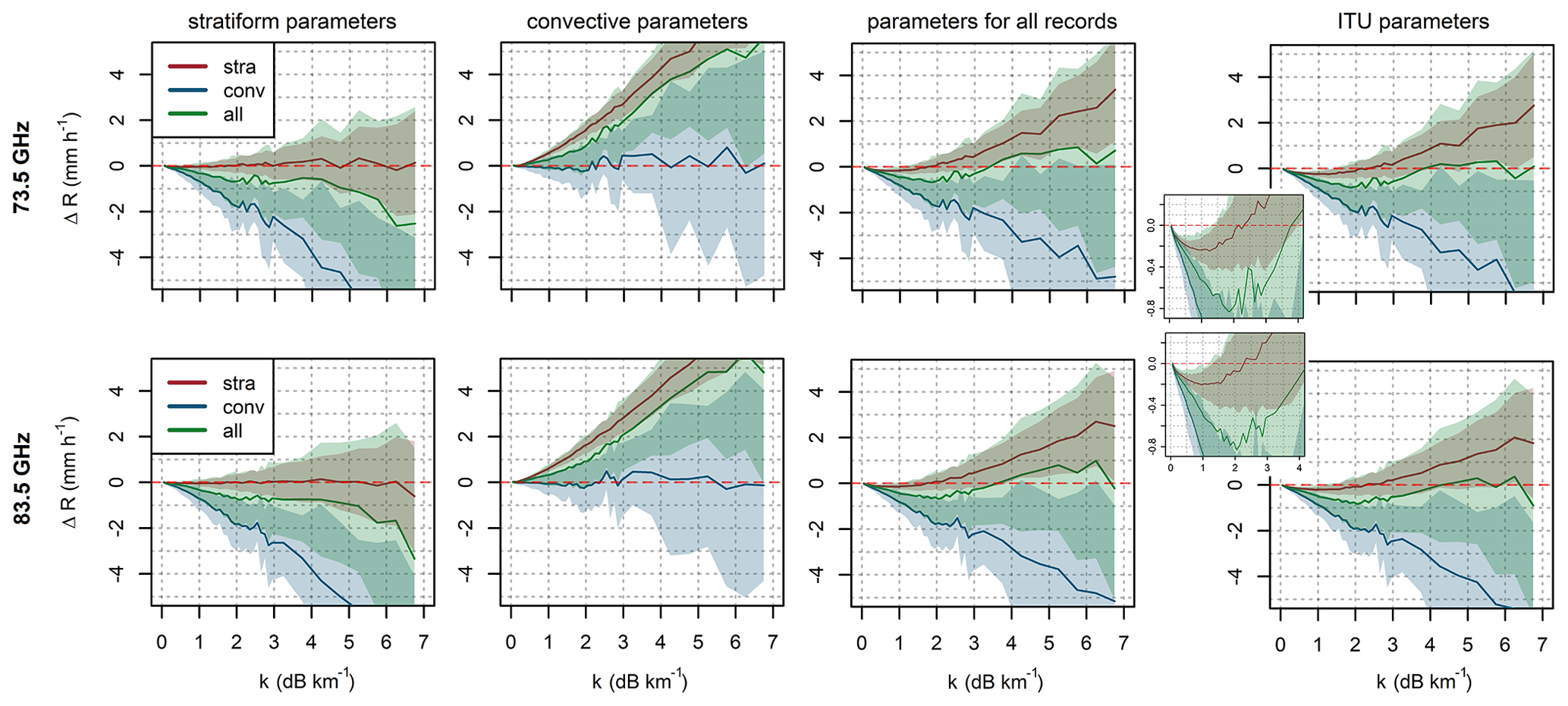
Figure 4Systematic deviation of the k–R models with different parameters from mean rainfall intensities when applied to (i) stratiform, (ii) convective, and (iii) all the rainfalls together. Random errors are depicted by bands corresponding to ± 1 standard deviation of rainfall intensities in a given bin. Insets show ITU model performance for the specific attenuation range of 0–4 dB km−1.
Figure 4 shows the expected systematic deviations and random errors of the k–R models (Eq. 9) with different parameters. Bands representing random errors are constructed for each attenuation bin as ± 1 standard deviation of rainfall intensities. Systematic deviations and standard deviations are evaluated for each rainfall class separately and then for both classes together. All four k–R models have similar patterns of deviation for the 73.5 and 83.5 GHz frequencies. The k–R model with stratiform and convective parameters is almost unbiased when used for the corresponding class of rainfalls. Nevertheless, any misclassification of rainfall can result in large errors, especially during higher rainfall intensities. The k–R model with parameters for convective rainfall is affected by substantial random errors. For example, for specific attenuation of 6 dB km−1, which corresponds to mean convective rainfall of approx. 8 and 9 mm h−1 for 73.5 and 83.5 GHz frequencies, respectively; the standard deviation reaches 4 mm h−1. The k–R models with ITU parameters and parameters optimized for all the rainfalls are with respect to systematic deviations more robust than stratiform and convective k–R models: nevertheless, they are affected by larger random errors. Noteworthy, the k–R model with ITU parameters and parameters optimized for all the rainfalls systematically underestimate light rainfalls including those classified as stratiform (Fig. 4, insets).
3.4 Analysis of wet antenna attenuation
Wet antenna analysis is performed on attenuation data after baseline separation aggregated to 15 min. WAA during rainfall is estimated by comparing attenuations as observed by sublinks of different path lengths. WAA quantification assumes spatially uniform rainfall under which specific attenuations k1, k2, …, kn (dB km−1) of the sublinks 1, 2, …, n operating at the same frequency band in the same area should be identical:
where Lr (dB) is rainfall-induced loss, i.e., the difference between total observed loss Lt and the baseline; Aw (dB) is wet antenna attenuation; and l (km) is CML (sublink) length. Assuming correct baseline identification and the same Aw for all CMLs, Aw can be directly quantified from any pair of sublinks of different lengths operating at the same frequency. The accuracy of the quantification relies on the fulfillment of the assumptions and the difference between the sublink lengths. The larger the length difference between the CMLs, the smaller the effect of an inaccurate baseline identification or dissimilar Aw within the CML pair. On the other hand, the assumption of spatially uniform rainfall is unlikely to be valid for CMLs covering a large area, i.e., with contrasting lengths.
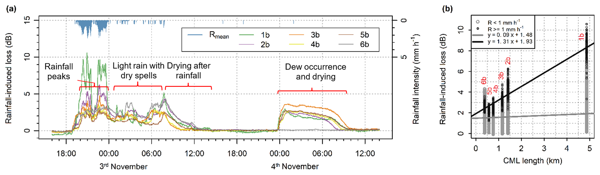
Figure 5(a) Rainfall-induced loss of 83–84 GHz sublinks and mean rainfall intensity from all four rain gauges. Period with peak rainfalls on 2 November from approx. 19:00 to 00:00 UTC, period with light rainfall and dry spells on 3 November from approx. 00:00 to 05:00 UTC, antenna drying period on 3 November from approx. 08:00 to 14:00 UTC, and dew occurrence and subsequent antenna drying on 4 November from approx. 00:00 to 10:00 UTC. (b) Rainfall-induced loss plotted against path length for 83–84 GHz sublinks with two separate linear fits for intervals with moderate rainfall and intervals with very light rainfall including dry spells. Period from 19:00 UTC on 2 November to 14:00 UTC on 3 November is shown.
WAA is quantified at each time step by comparing the rainfall-induced losses of the short CMLs to the losses of the long CML. WAA after rainfall and during dew events is assumed to be equal to the total rainfall-induced loss. Figure 5 presents CML data at a 1 min temporal resolution featuring (i) attenuation during peak rainfall, (ii) attenuation during dry spells at night on 3 November and after the rainfall, and (iii) attenuations during dew occurrence on the morning of 4 November. Rainfall-induced loss during peak rainfall is markedly influenced by raindrop path attenuation and is proportional to path length (Fig. 5b). In contrast, rainfall-induced loss, both during dry spells and after rainfall as well as during dew occurrences (except sublink 6b), is dominated by WAA and thus independent of path length. Therefore, the WAA quantification method utilizing different CML path lengths seems to be conceptually justified.
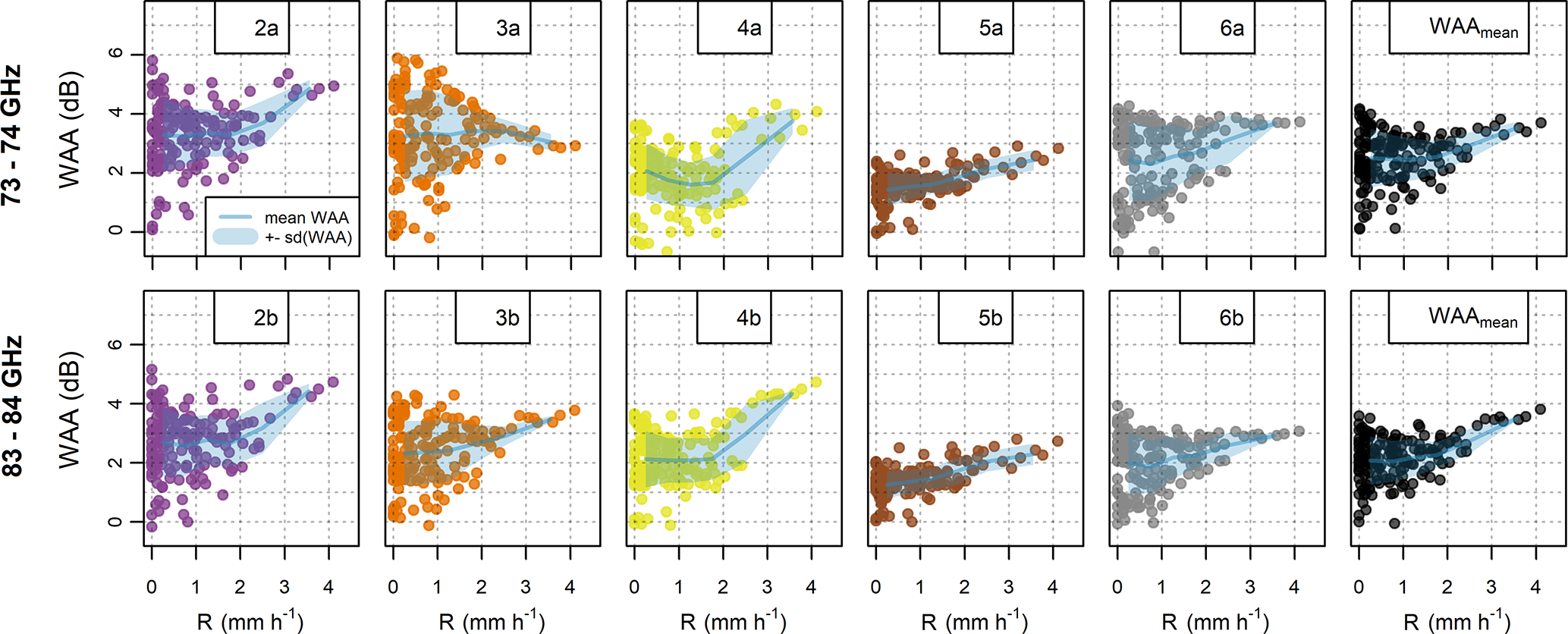
Figure 6Wet antenna attenuation during rainfall estimated from the differential attenuation of short and long CMLs. WAAs with their mean and standard deviation are shown for both sublinks (73–74 and 83–84 GHz) of CMLs 1–5. The panels on the right side show mean WAA for all CMLs.
WAA quantified for each shorter CML and their average is shown in Fig. 6 at a 15 min temporal resolution. WAA is related to mean rainfall intensity from rain gauges at sites 1, 2, and 4 and subdivided into bins of size 0.5 mm h−1 for light rainfalls under 2 mm h−1 and bins of size 1 and 1.1 mm h−1 for higher rainfall intensities of 2–3 mm h−1 and 3–4.1 mm h−1, respectively, which are sparse in our dataset. Mean WAA and its standard deviation are quantified for each bin. Higher rainfall intensities are, in general, associated with high WAA, whereas WAA reaches a wide range of values during lower intensities. Mean WAA for rainfall intensities lower than 0.5 mm h−1 reaches 1.4–3.3 dB with standard deviations of 0.6–1.3 dB for the 73–74 GHz sublinks and 1.3–2.7 dB with standard deviations of 0.5–1.2 dB for the 83–84 GHz sublinks. Similar values are obtained when evaluating mean WAA and standard deviation over the whole evaluation period: mean WAA is between 1.6 and 3.4 dB with standard deviations of 0.5–1.3 dB for the 73–74 GHz sublinks and 1.4–2.8 dB with standard deviations of 0.5–1.1 dB for the 83–84 GHz sublinks. WAA correction used during rainfall retrieval considers WAA as being a constant. It is determined as the median value of WAAs quantified separately for the 73–74 GHz and 83–84 GHz sublinks, respectively. This simple approach might lead to systematic under- or overestimating of rainfall-induced loss in about 1 dB and random errors corresponding to standard deviations reported above.
Further, inspection of CML time series reveals an exponential decrease of attenuation after rainfall, which is probably due to the drying of the antennas (Fig. 5a, 3 November). WAA also contributes to total attenuation during the occurrence of dew when water condensates on the antenna radomes. Attenuation associated with dew deposition is similar for both frequency bands and reaches up to 4 dB (Fig. 5a, 4 November morning). These values are higher than WAA caused by rainfall.
3.5 Water vapor detection
The detection of water vapor from CML observations relies strongly on the ability to separate gaseous attenuation from other losses. The evaluation presented in this study is limited to this aspect. The effect of temperature and air humidity on total CML attenuation is estimated theoretically from observed air temperature and relative humidity (see Sect. 2.2) and compared to the real CML data obtained during the case study from the long CML (ID 1). Atmospheric pressure was not measured and is assumed to be constant corresponding to 1013 hPa. Atmospheric pressure changes related to weather conditions have, however, an almost negligible effect on theoretical attenuation (ITU-R, 2019). The temperature and air humidity used in the analyses are averages from the observations at two locations along the CML path. Gaseous attenuation is estimated for the period from 20 August to 16 December 2018 and only considers dry weather, as defined in Sect. 3.2.
The theoretical attenuation derived from air temperature and relative humidity observations is compared to the observed attenuation of the long CML. To enable a comparison, the observed attenuation is also aggregated to a 5 min time step corresponding to the time step of temperature and humidity observations and theoretical attenuation, respectively.
The observed attenuation patterns are compared to the theoretical patterns calculated from temperature and air humidity observations. The agreement between theoretical and observed attenuation is quantified in terms of correlations, mean difference, root-mean-square error (RMSE), and their amplitudes. In addition, seasonal drift is demonstrated on time series smoothed by a moving average with a window size of 1 week.
3.6 CML rainfall retrieval
Rainfall is estimated for each sublink using the k–R power-law model (Eq. 9) with ITU parameters and parameters derived from DSD observations (Duebendorf data) classified as stratiform rains, alternatively. The parameters for stratiform rainfalls are used for its dominance in light and moderate autumn rainfalls in the Czech Republic. The CML quantitative precipitation estimates (QPEs) of the long CML are compared to average 15 min rainfall from rain gauges at sites 1, 2, and 3. The QPEs of the short CMLs are compared to average 15 min rainfall from rain gauges at sites 1, 2, and 4. The quantitative evaluation focuses on the long CML, which is sufficiently long to capture even the light rainfalls dominating the Prague data. The performance of the short CMLs is shown to demonstrate limitations related to the inappropriate baseline and WAA identification which are, especially during light rainfalls, more pronounced by shorter CMLs. The CML QPEs are evaluated over selected rainfall events (Table 2) in terms of correlation, relative error in cumulative rainfall, and RMSE.
Uncertainty estimation. CML QPEs are subdivided into bins having size 0.5 mm h−1 for light rainfalls under 2 mm h−1; two other larger bins (2–3 and 3–4.1 mm h−1) are defined for higher rainfall intensities, which are sparse in our dataset. Average difference between CML QPEs and mean rain-gauge rainfall and standard deviations of residuals are then quantified for each bin. Evaluation of DSD-related deficits of k–R model is, for simplicity, limited to the k–R model with ITU parameters and assumes that drop size spectra of rainfalls during the evaluation period resemble Duebendorf DSD classified as stratiform. Expected systematic and random deviations of the k–R model with ITU parameters are quantified in Sect. 3.3 for bins of specific attenuation. Nevertheless, these bins need to be transformed to rainfall intensity to enable comparison with quantified deviations of CML QPEs. Equation (9) with parameters for stratiform rainfalls is used for this purpose. The estimation of WAA-related deficiencies is limited to systematic errors and assumes that the WAA offset (2.3 and 2.7 dB) might be for any CML systematically under- or overestimated by ± 1 dB. First, CML QPEs are calculated for specific attenuations in the range of 0–4 dB km−1 using the k–R model (Eq. 9) with parameters for stratiform rainfalls. Second, the systematic deviation ± 1 dB is introduced into Eq. (3) and systematically under- and overestimated QPEs are calculated (Eq. 9) for each CML considering differences in their path lengths. Difference between unbiased QPEs (corresponding to mean rain-gauge rainfall) and under- and overestimated QPEs is quantified and related to rainfall intensity.
4.1 Gaseous attenuation – effect of air humidity and temperature
Theoretical gaseous attenuation calculated from observed temperatures and relative humidity is positively correlated to water vapor density (r=0.94–0.97) at both frequencies studied. The fluctuations in temperature affect this relation negligibly. The further evaluation, therefore, concentrates on the comparison of theoretical attenuation to attenuation observed by two sublinks of the long CML 1. To separate gaseous attenuation from other possible attenuations, only dry-weather periods are evaluated.
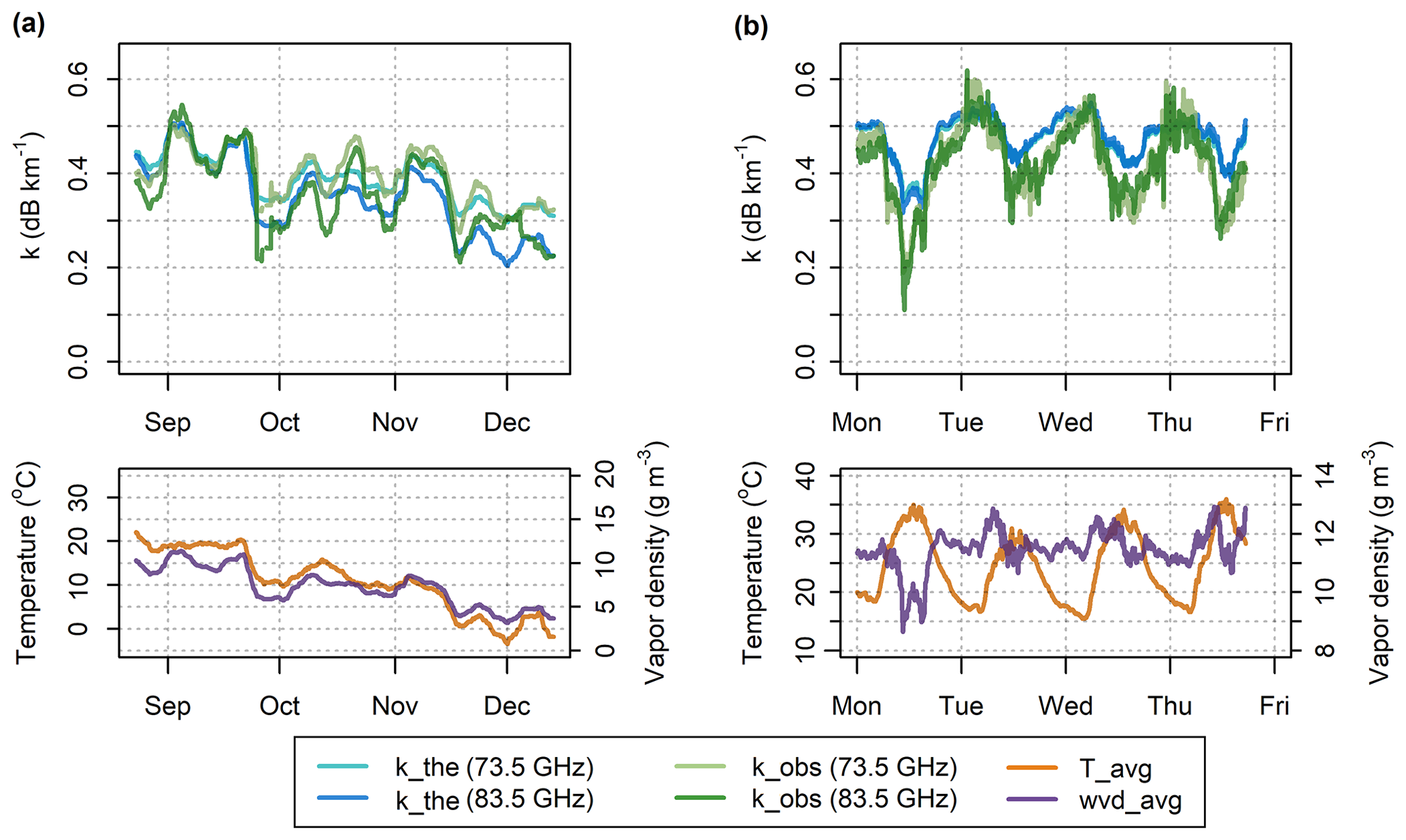
Figure 7Theoretical and observed specific attenuation from the 73.5 and 83.5 GHz sublinks of CML 1 and observed temperature and water vapor density – (a) data over the whole observation period smoothed by a moving average with 1-week window and (b) 5 min data during four summer days.
Time series of theoretical and observed attenuation are compared in Fig. 7, which shows time series of specific attenuations smoothed by a moving average (1-week window size). The correlation between theoretical and observed attenuation is high for both sublinks (r=0.82–0.83) and the long-term patterns of observed and theoretical attenuations correspond to each other quite well. Both theoretical and observed attenuations are higher during the summer period (August–September) and gradually decrease during the autumn period (October–December). The difference between mean attenuation levels in August and December is about 0.15 dB km−1 for the 83.5 GHz sublink compared to only 0.12 dB km−1 for the 73.5 GHz sublink. The theoretical and observed attenuations have similar median values for both frequencies during summer (0.44 and 0.43 dB km−1 for 73.5 GHz and 0.43 and 0.42 dB km−1 for 83.5 GHz, respectively). The theoretical and observed attenuations during autumn are about 0.06 dB km−1 higher for 73.5 GHz compared to the 83.5 GHz sublink (0.37 and 0.40 dB km−1 for 73.5 GHz compared to 0.32 and 0.33 dB km−1 for 83.5 GHz, respectively).
The higher attenuations of the 73.5 GHz sublink during the autumn period, in comparison to the 83.5 GHz sublink, can be explained by dry-air attenuation. Dry-air attenuation of 73.5 GHz is about 0.04–0.06 dB km−1 higher (depending on temperature) than that of 83.5 GHz. On the other hand, higher-frequency bands are more sensitive to water vapor attenuation, which is higher during the summer. Different sensitivity to water vapor attenuation also causes more significant seasonal drift in the attenuation of the 83.5 GHz sublink compared to the 73.5 GHz one.
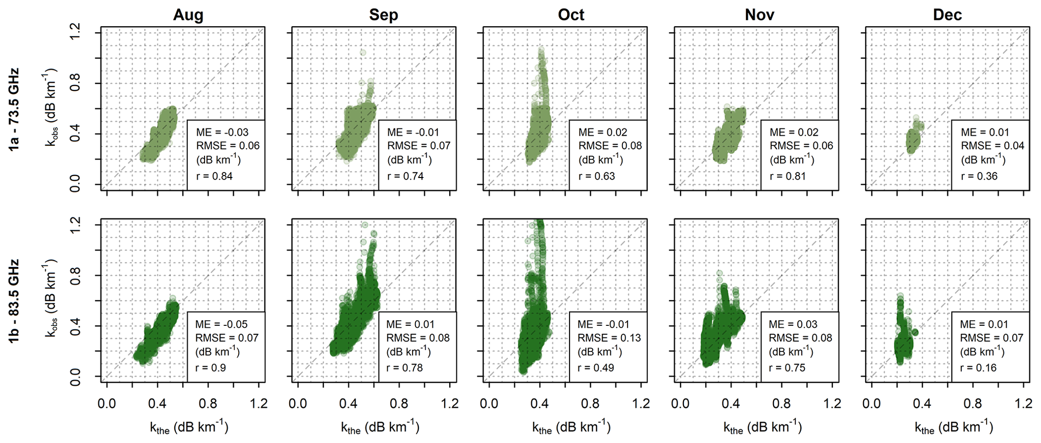
Figure 8Comparison of theoretical (x axis) and observed (y axis) gas-specific attenuations at the 73.5 and 83.5 GHz sublinks of CML 1 for 5 min data. Data are shown separately for each month.
The discrepancies between theoretical and observed attenuations are more pronounced when analyzing data at a 5 min resolution, as demonstrated on the time series of four summer days shown in Fig. 7b. This is because the separation of gaseous attenuation from the other sources of attenuation or hardware-related artifacts is challenging in real conditions. Despite these discrepancies, the correlation between theoretical and observed attenuations remains relatively high (r=0.70–0.72). The theoretical and observed attenuations are highly correlated during August (Fig. 8), with the correlation coefficients reaching 0.84 and 0.90 for the 73.5 GHz and 83.5 GHz sublinks, respectively. The correlation is lowest during December (r=0.36 and 0.16, respectively). On the other hand, systematic deviations are largest during August, where observed attenuation of 73.5 and 83.5 GHz sublinks is underestimated by 0.03 and 0.05 dB km−1, respectively compared to theoretical attenuation. RMSE is for both sublinks largest during October (0.08–0.13 dB km−1). Possible causes of outlying observed attenuations causing high RMSEs are discussed in Sect. 5. The lowest RMSE is quantified for the 73.5 GHz sublink during December and for the 83.5 GHz sublink during August.
4.2 Rainfall estimation
Figure 9 shows QPEs obtained from CMLs using the k–R model with ITU parameters and parameters derived from DSD during rainfalls classified as stratiform. Note that DSD is obtained from the independent Duebendorf dataset. The long CML, in particular the 83.5 GHz sublink, is capable of capturing even light rainfall intensities reliably. The correlation to rain-gauge observations is excellent (r≈0.96). However, QPEs derived with ITU parameters tend to underestimate light rainfalls, leading to increased RMSE (Table 3). The model with DSD-derived parameters improves performance with respect to all metrics. Sublink 1a also remains significantly underestimated with DSD-derived parameters. The underestimation is pronounced especially during very light rainfalls with rainfall intensities under 1 mm h−1, which represent 25 % of total rainfall depth. The use of DSD parameters does not significantly improve the performance of short CMLs and CMLs shorter than 1 km overestimate rainfall intensities more than longer CMLs.
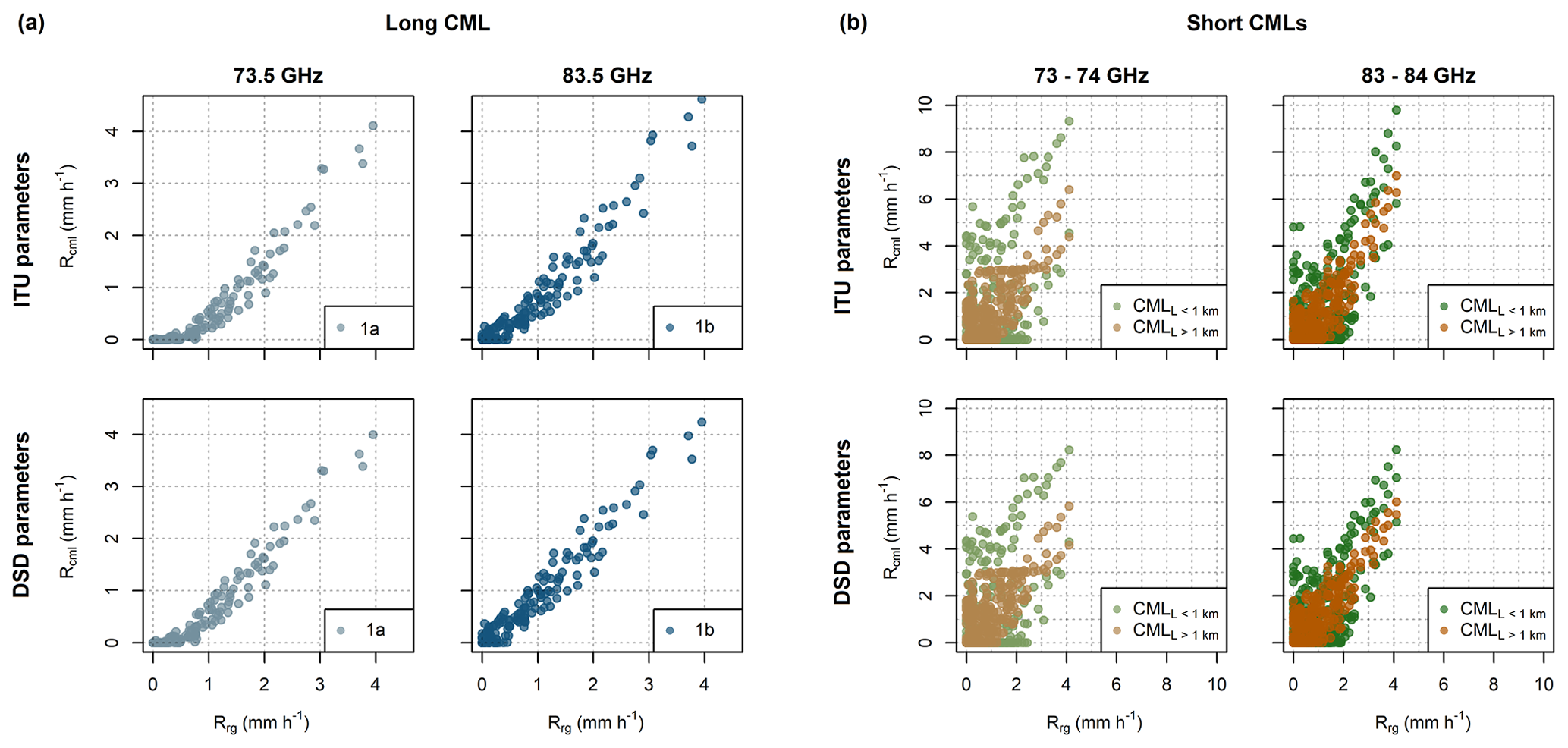
Figure 9CML QPEs for the long CML (a) and short CMLs (b) when using the k–R model with ITU (top) and DSD-derived (bottom) parameters. Results are shown for both frequency ranges. QPEs for short CMLs are differentiated by color into two groups to depict CMLs with path lengths shorter and longer than 1 km separately.
Table 3Performance metrics of the CML QPEs obtained with the k–R model using ITU and DSD-derived parameters.
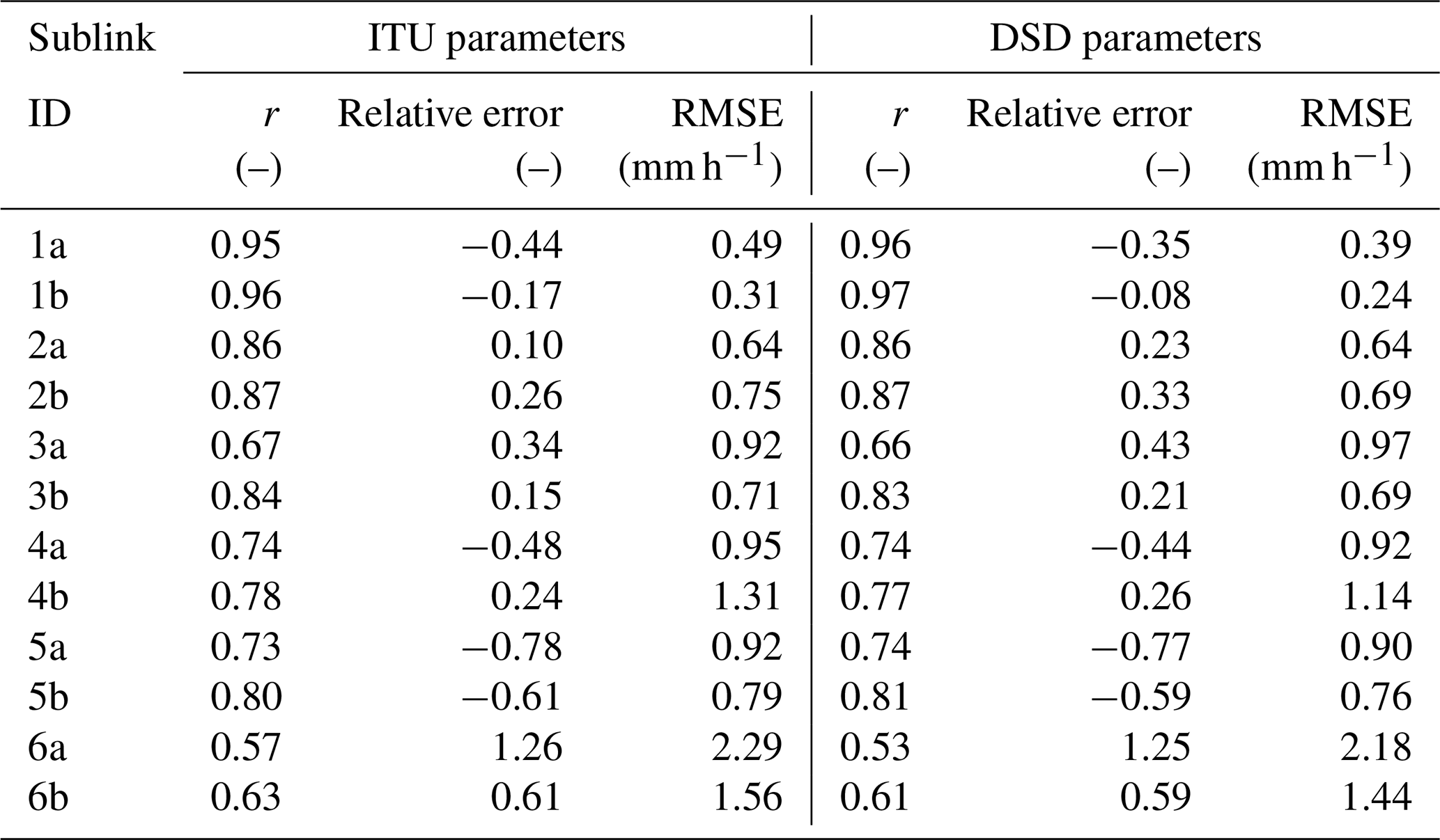
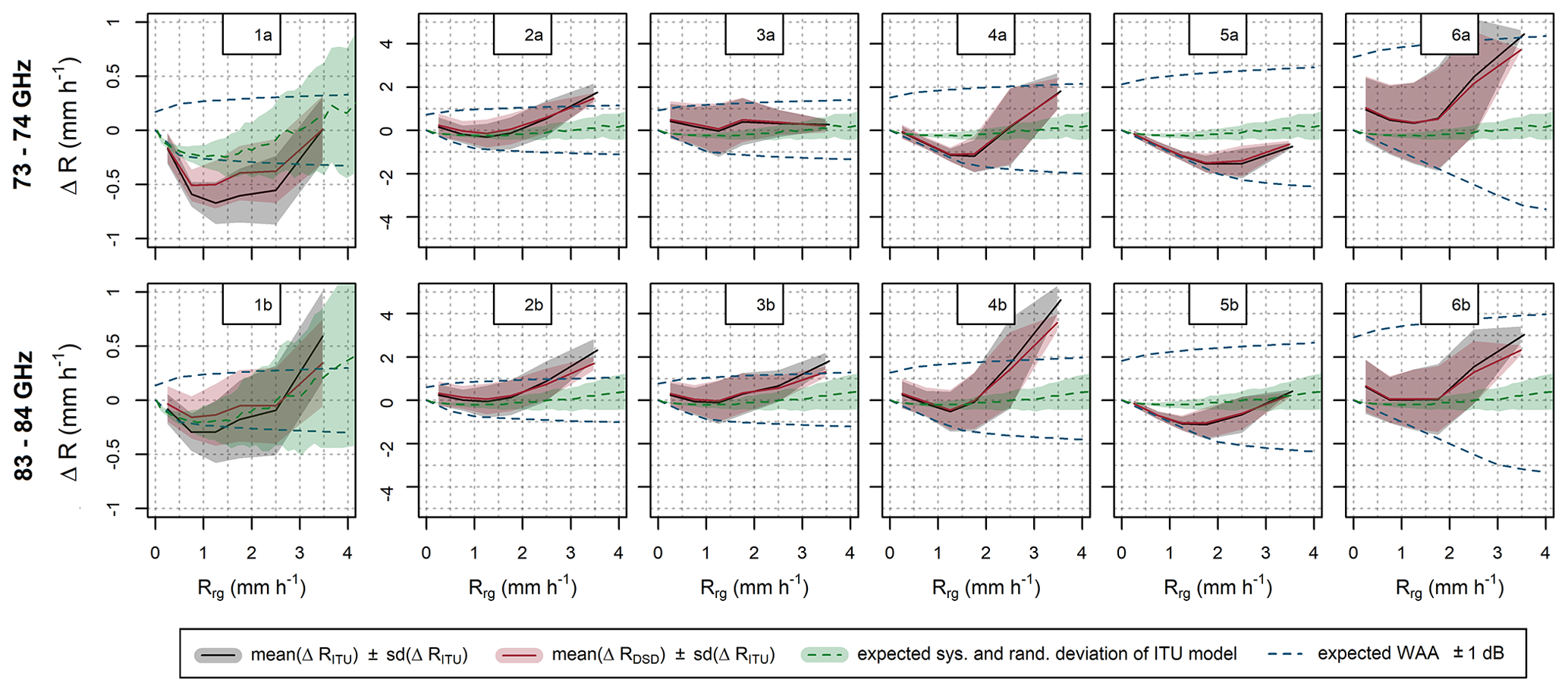
Figure 10Deviations of CML QPEs when using the k–R model with ITU parameters and DSD-derived parameters for stratiform rainfalls. Expected deviations due to DSD and deficits in the constant WAA model are also shown. Note the different scale of y axis for the long (1a, b) and the short (2–6a, b) sublinks.
Systematic and random deviations of CML QPEs are evaluated quantitatively in Fig. 10 and compared to expected systematic and random deviations (i) due to deficits of the constant WAA model and (ii) due to DSD-related deficits of the ITU-based model. The expected errors due to DSD are independent of CML path length and contribute equally to all the CMLs. In contrast, expected errors due to WAA are much more pronounced by the shorter CMLs and can explain most of their errors. Regarding the 4.86 km long CML, DSD seems to affect deviations of QPEs similarly or even more (for the 83.5 GHz sublink) than WAA. DSD-related errors might explain a substantial part of observed systematic deviations by this CML. Interestingly, expected random error due to DSD variability is even larger than the observed variability in QPEs during rainfalls intensities higher than approx. 2–3 mm h−1. Note that observed variability for rainfall intensities higher than 3 mm h−1 is quantified based on five observations only by the longest CML.
In general, sensitivity to rainfall, which is proportional to a CML path length, seems to be a crucial characteristic influencing the accuracy of CMLs when observing light rainfalls under 2 mm h−1. For heavier rainfalls, other characteristics than path length specific to each CML influence the uncertainties more significantly. For example, CML 5, which is less biased than longer CML 4, is relatively insensitive to WAA (Fig. 6) compared to the other CMLs. In addition, the WAA quantified for CML 5 is more correlated with rainfall intensity (r=0.47 and 0.54 for the sublink 5a and 5b, respectively) than by the other CMLs (r=0.23–0.40 for all the sublinks).
Quality check before rainfall retrieval. A quality check was performed by visually inspecting time series of total losses. In the case of CML 2, a sudden change in the baseline by 2 dB was manually corrected. More details on hardware-related artifacts are provided in Appendix B.
Dry–wet weather classification and baseline separation. The dry–wet classification has been reported as an important step in CML preprocessing as it minimizes unwanted changes in attenuation level by setting the baseline separately for each event from the relatively short period before the event (Chwala and Kunstmann, 2019; Overeem et al., 2011). Here, dry–wet weather classification was not used for baseline identification when retrieving rainfall. It was a pragmatic choice enabling better descriptions of the WAA effect. Dry–wet classification is also needed for filtering out periods with increased attenuation due to WAA (after rainfall and during dew events); nevertheless, these periods are in the event-based evaluation not included.
The separation of wet weather (including dew occurrence) was identified as a crucial step when analyzing attenuation due to water vapor. When rain gauges are not available, a CML-based classification needs to be performed. The dry–wet weather classification (Schleiss and Berne, 2010) used in Appendix A is designed to identify rainy periods and consider dew occurrences as dry weather. Although sensitivity to dew events can be increased by optimizing the parameters of the algorithm, dew events have similar dynamics as changes in air humidity as they are both dependent on temperature. Thus, other methods also considering observations of neighboring CMLs (Overeem et al., 2011) might be more appropriate for the dry–wet weather classification used to separate attenuation caused by water vapor.
The baseline identification method with a moving median (without dry–wet weather classification) performed well for rainfall retrieval purposes. It should be noted that, except for one case, the observed attenuation levels were stable. The baseline identified by moving median with a 1-week window was capable of correcting long-term drift, which occurred on sublink 6a (Appendix B). A 1-week window is sufficiently long to not include more than 50 % of wet weather records into the window at any time step in the temperate climate. However, the median moving window baseline is not suitable for distinguishing between long-term drift related to hardware malfunction (e.g., sublink 6a) and drift related to seasonal changes in air humidity and temperature (sublinks 1a and 1b). A constant baseline was, therefore, used for analysis of gaseous attenuation on sublinks 1a and 1b instead. Possible water vapor monitoring thus poses higher requirements on the hardware with respect to the stability of the attenuation baseline.
Accuracy of the k–R power-law approximation. The relation between rainfall and raindrop attenuation (Eqs. 8 and 9) on E-band frequencies is substantially more dependent on DSD than on 15–40 GHz CMLs (Chwala, 2017). The parameters of the power-law model (Eq. 9), when optimized for all the DSD data, corresponds exceptionally well to the ITU parameters (ITU-R, 2005). However, random errors resulting from the variability in DSD are high when using one fit for all the records. Separate fits for convective and stratiform rainfalls reduce these errors. Moreover, the separate power-law fits are closer to linear (parameter β between 1.18 and 1.26 compared to β between 1.38 and 1.4) and are less prone to errors related to nonuniform rainfall distribution along the CML path. On the other hand, high systematic errors will occur for misclassified rainfall type (DSD). Errors due to nonlinearity of Eq. (9) might be reduced by reconstructing rainfall spatial variability along the CML path from the neighboring CMLs or by introducing a climate-based relation between the nonuniformity of rainfall distribution and rainfall intensity. Such methods will, however, require further research. In general, unknown DSD will probably be one of the significant uncertainties in quantitative estimates of heavy rainfall. On the other hand, high sensitivity to DSD creates the opportunity to infer information on DSD from the attenuation of E-band CMLs, e.g., in a condensed form of DSD moments. This is, in theory, also possible at 15–40 GHz, though it is challenging to accomplish in practice (van Leth et al., 2020). Additional information on rainfall intensity or a combination with attenuation data of CMLs operating at lower frequencies will be required for DSD retrieval.
Quantification of wet antenna attenuation. Quantification of WAA during rainfall is based on the assumptions that rainfall has a uniform distribution over the study area and that water formation on the surface of antenna radomes is the same for both the short CMLs and the long one. In our case, the first assumption holds well as all four rain gauges observe similar rainfall intensities during the evaluated events. The correlation coefficients between rain gauges at sites 1, 2, and 4, which are closer to each other, are 0.94–0.96, and they are 0.88–0.93 for the more distant rain gauge at site 3. The standard deviation between mean rainfall intensity and rainfall intensities observed by single rain gauges reaches 0.15–0.36 mm h−1, being lowest for the lightest rainfalls and slightly grows with increasing rainfall intensity. The similarity in antenna characteristics, i.e., hydrophobic properties of antenna radomes and their actual status, was not inspected directly. That said, the estimation procedure is relatively insensitive to WAA occurring on the long CML as attenuation along its path dominates over WAA, even during relatively light rainfalls; thus, WAA does not significantly influence the estimated specific attenuation (Eq. 3).
WAA during rainfall is weakly correlated to rainfall intensity (e.g., Schleiss et al., 2013). Our results are limited to light and moderate rainfall only. Schleiss et al. (2013) reported drying of up to 6 h with an exponential decrease of WAA, which also corresponds well to our observations (Fig. 5a). However, quantification of exact duration of drying requires additional instrumentation to enable us to determine the ends of rainfalls directly. The exponential WAA decrease during drying was also reported by van Leth et al. (2018), who suggested that this drying pattern occurs on antennas with nondegraded coating, which is also the case of the CML antennas analyzed. On the other hand, WAA attenuation patterns on antennas with degraded coating might be markedly different.
WAA, due to water vapor condensation, reaches higher values than during light rainfall. This might be caused by the absence of water rivulets (van Leth et al., 2018). The higher values of attenuation caused by water droplets, in comparison to attenuation caused by rivulets, was also reported by Mancini et al. (2019). Comparable attenuation patterns of light rainfall and water vapor condensation may cause the misclassification of dew as rainfall.
In general, WAA quantified in this study is slightly higher than WAA reported for lower frequencies (van Leth et al., 2018). However, the relative contribution of WAA to the total attenuation is less significant (given the high sensitivity of CMLs to raindrop path attenuation). WAA is thus a smaller source of possible bias than on 15–40 GHz frequencies. Nevertheless, accurate quantification of WAA is still essential, especially for shorter CMLs. In addition, WAA during heavy rainfalls was not investigated in this study and might be higher, as was shown for lower frequencies by Fencl et al. (2019).
Gaseous attenuation. The theoretical gaseous attenuation for the 73.5 GHz sublink ranges between 0.27 and 0.60 dB km−1 (amplitude 0.33 dB km−1) and for the 83.5 GHz sublink between 0.20 and 0.63 dB km−1 (amplitude 0.43 dB km−1). These fluctuations have a minor effect on rainfall retrieval (with respect to uncaptured baseline variability), as 0.33 and 0.43 dB km−1 correspond to rainfall intensities of about 0.19 mm h−1 and 0.25 mm h−1, respectively, for 73.5 and 83.5 GHz sublinks. On the other hand, this signal is sufficiently strong to enable the detection of water vapor at long CMLs, as 0.33 and 0.43 dB km−1 correspond to 1.60 and 2.09 dB, respectively, for the long CML (4.86 km). The major challenge lies in the separation of gaseous attenuation from losses caused by other phenomena. This is easier during periods without rainfall; nevertheless, the following causes of losses need to be identified and separated.
First, WAA occurring after rainfall and during dew events can reach 4 dB, i.e., substantially exceeds the gaseous attenuation. Here, a safety window of 6 h was used before and after each rain-gauge tipping to exclude periods with WAA contribution. This mostly eliminated WAA before and after rainfall events and WAA during strong dew events causing a rain-gauge tip. However, such eliminations considerably reduce the ratio of time intervals with observations. Moreover, periods before and after rainfalls might have higher relative humidity than average and discarding those from the evaluation leads to potentially biased long-term estimates of water vapor density.
Second, signal fluctuations due to multipath propagation or other sources of uncertainty might affect the observed attenuation level. Multipath interferences often lead to a decreased signal power level of one sublink while keeping the signal power level of the other sublink (Valtr et al., 2011).
Finally, hardware-related artifacts might destroy a gaseous attenuation signal. For example, sublink 6a drifts about 1.5 dB from the end of October to mid-December. This drift is clearly related to the hardware as the total loss due to gaseous attenuation along the path length of 0.39 km can reach only about 0.13 dB. Such a drift would, however, make the quantification of gaseous attenuation impossible even at long CMLs.
The separation of gaseous attenuation from other sources of signal loss is challenging. Further research could take advantage of the 10 GHz duplex separation between the sublinks of E-band CMLs. Combining attenuation information from CMLs of different lengths might also be promising.
Rainfall estimation. The E-band CMLs proved to be markedly more sensitive to raindrop path attenuation than 15–40 GHz devices. The long CML provided surprisingly accurate rainfall estimates, even for light rainfalls lower than 1 mm h−1 in intensity (Fig. 9). Assuming a detection threshold of 1 dB (typical tx power quantization of older devices), a 1 km long 83 GHz CML can already detect rainfall intensity of 0.6–1 mm h−1, depending on rainfall type, whereas, for example, a 23 or 38 GHz CML only detects rainfalls heavier than 8.4 or 3.6 mm h−1, respectively; i.e., the sensitivity to light rainfalls is almost an order of magnitude higher for E-band CMLs. Moreover, the quantization of rx and tx records has improved to 0.1 dB with E-band CMLs. On the other hand, long E-band CMLs are prone to outages (rx drops under detection level) during heavy rainfall.
This high sensitivity to rainfall, together with improved quantization, opens the opportunity for monitoring rainfall with CMLs having a sub-kilometer path length, which was practically impossible in the past without adjusting CML QPEs to the rain gauges (Fencl et al., 2017). Short CMLs are more affected by errors related to WAA, yet the influence of WAA is relatively smaller during heavier rainfall, which, however, did not occur during the evaluation period. The use of short CMLs may be convenient, especially during heavy rainfalls associated with high spatial variability by which an assumption about uniform rainfall distribution along a CML path is more likely valid than for long CMLs. Reliable rainfall estimation from short CMLs, however, requires further research on WAA modeling at E-band frequencies.
Limitations of this study. The study investigates the weather-monitoring capabilities of E-band CMLs on a dataset comprised of 4 months of attenuation data from six Ericsson MINILINK CMLs operated within cellular backhaul. The number of CMLs and length of the period is sufficient to demonstrate the challenges and opportunities related to rainfall and water vapor monitoring at E-band frequencies. However, the limited size of the dataset does not enable us to draw strong conclusions on the overall reliability of weather monitoring with an E-band CML nor to investigate in detail new opportunities related to CML sensitivity to water vapor and DSD.
Specifically, the dataset does not include heavy rainfalls. The reliability of E-band CML rainfall estimation for heavy rainfalls is based only on evaluating theoretical attenuations obtained from DSD observations (Duebendorf). The DSD effect on the attenuation–rainfall relation could not be studied in detail on the observed CML data. Finally, air temperature and humidity are measured at two locations close to one node of the CML path. Despite these limitations, we believe that the presented results reliably demonstrate new challenges and opportunities of E-band CML weather monitoring.
E-band microwave links are increasingly being updated and are frequently replacing the older hardware of backhaul networks operating mostly at 15–40 GHz. This investigation demonstrates new challenges and opportunities related to CML weather monitoring. The principles behind weather retrieval are the same as for lower-frequency bands; nevertheless, the influence of atmospheric phenomena such as drop size distribution or changes in air temperature and humidity affect radio-wave propagation in a significantly different manner. Furthermore, the hardware used by E-band CMLs is different (quantization, accuracy, antenna wetting, etc.). The results, obtained from simulations and the case study with attenuation data from real-world CMLs, are encouraging. The main conclusions are listed below:
-
E-band CMLs are markedly more attenuated by raindrops along their path than older 15–40 GHz devices, during lighter rainfalls by about 20 times more than 15 GHz and 2–3 times more than 40 GHz devices. This significantly improves the ability of E-band CMLs to quantify rainfall intensity accurately during light rainfalls.
-
The rainfall retrieval at E-band frequencies is less influenced by wet antenna attenuation than at lower frequencies. WAA observed in this study has a similar pattern as that described by Schleiss et al. (2013); i.e., it is almost uncorrelated with rainfall intensity and exhibits an exponential decrease after rainfall lasting up to several hours. WAA during dew occurrences reaches up to 4 dB.
-
The power-law approximation of the attenuation–rainfall relation depends substantially more on DSD than on 15–40 GHz frequencies. The variability in DSD represents a significant uncertainty in E-band CML rainfall retrieval. The use of different parameter sets for different types of rainfall, as done with weather radars, reduces DSD-related errors; nevertheless, this requires additional information on rainfall type.
-
The k–R relation at E-band frequencies is less linear than at lower frequencies. This might cause errors in CML QPEs, especially by longer CMLs, for which a uniform distribution of rainfall intensity along their path cannot always be assumed. On the other hand, even short (sub-kilometer) E-band CMLs are sufficiently sensitive to raindrop path attenuation for rainfall retrieval.
-
Gaseous attenuation at E-band CMLs is detectable; however, it is substantially lower than attenuation due to rainfall. Fluctuations in specific attenuation caused by water vapor typically do not exceed 1 dB km−1 in temperate climate regions. This magnitude is reached by rainfall with an intensity of around 1 mm h−1. Gaseous attenuation is driven mainly by water vapor density and is thus, in theory, an accurate predictor of this atmospheric variable. This, however, requires the efficient separation of attenuation from other signal losses which is, in practice, challenging. Our first results show that this separation is, to some extent, possible during dry weather periods when a sufficiently long CML (several kilometers) is available.
In general, the ongoing shift of CML networks towards higher frequencies creates opportunities to monitor rainfall on a qualitatively different level. New E-band CMLs can observe light rainfalls and, in combination with lower-frequency CMLs, potentially serve as DSD predictors. The rainfall retrieval methods developed for CMLs operating at 15–40 GHz frequencies proved to be useful for E-band CMLs. Water vapor retrieval from E-band CMLs having path lengths of several kilometers might be possible. However, the efficient separation of gaseous attenuation from other signal losses will be challenging in practice. This first experience with E-band CML weather retrieval, as presented in this study, will hopefully contribute to more robust designs of future experimental studies and case studies investigating this new technology concerning weather monitoring.
The classification is performed separately for each sublink on quality-checked total observed losses. The algorithm of Schleiss and Berne (2010) is used which is based on a moving window standard deviation. The window size is set to 15 min, and the threshold for classifying the record as wet (σ0) is set to the 94 % quantile of all standard deviations resulting from the moving window filter. The 94 % probability corresponds approximately to the wet weather ratio in the Prague data classified by the rain gauges.
Dry–wet weather classifiers obtained from CML sublinks are compared with each other and with classifiers obtained from rain-gauge observations. Correlation is used here as a measure of similarity. The evaluation of dry–wet weather is performed on 1 min data, because precise identification of the onset and ending of rainfall significantly affects baseline identification methods based on dry–wet classification, as well as the quantification of wet antenna attenuation.
Dry–wet weather classifiers of single sublinks belonging to one CML are strongly correlated (Fig. A1). An exception is sublink 4a, which is affected by a hardware malfunction (Appendix B). The correlation between the classifiers of sublinks belonging to different CMLs is lower but still reaches high values ranging between r=0.57 and r=0.84. The correlation of CML classifiers to the classifiers based on rain gauges is, on average, slightly lower (r=0.57–0.67).
The evaluation of dry–wet weather classification is only approximate, because tipping bucket rain gauges are unable to detect the exact beginning or end of a rain event. Visual inspection of time series reveals that disagreement between rain gauges and CMLs occurs most commonly during dew events and during periods of low temperature where mixed or snow events probably occur. Although sensitivity to dew events can be increased by optimizing the parameters of the algorithm, dew events have similar dynamics as changes in air humidity as they are both dependent on temperature. Thus, other methods also considering observations of neighboring CMLs (Overeem et al., 2011) might be more appropriate for the dry–wet weather classification used to separate attenuation caused by water vapor.
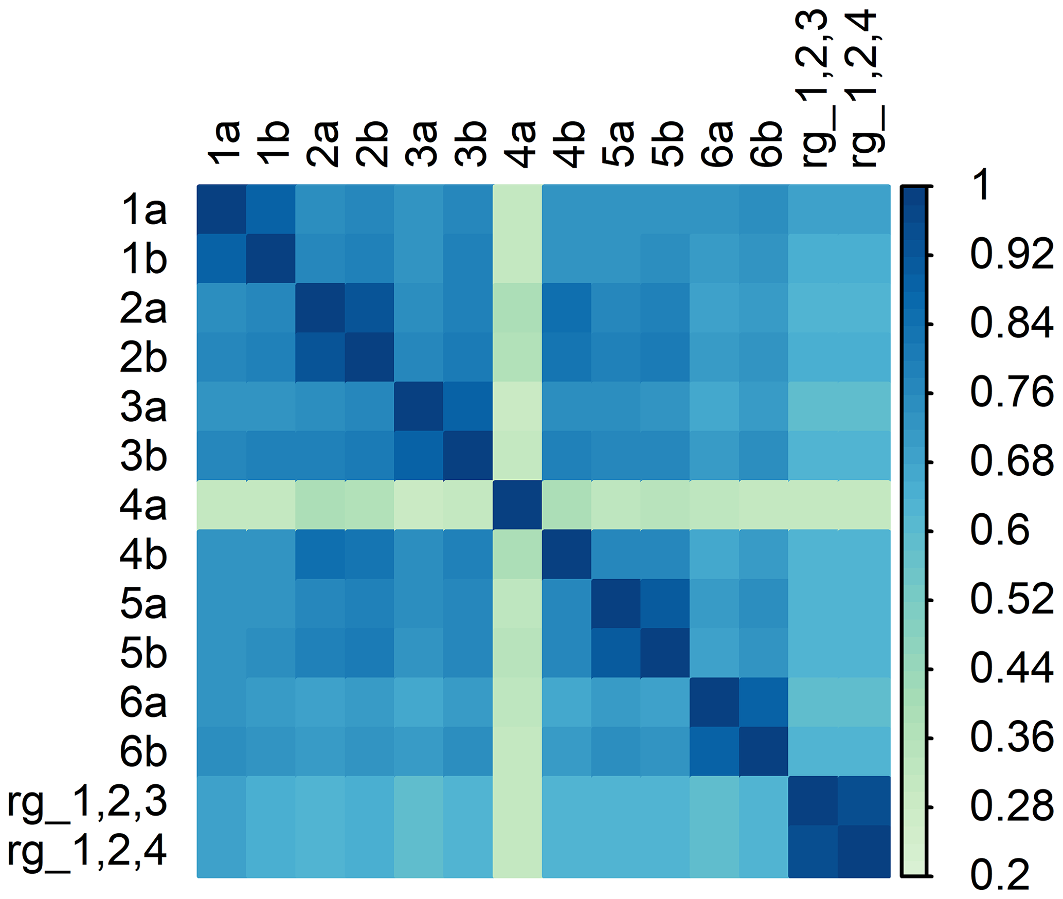
Figure A1Statistical relationship between dry–wet classifiers based on single CML sublinks and rain gauges along the path of the long CML (rg_1,2,3) and three rain gauges near five shorter CMLs (rg_1,2,4) expressed by correlation coefficient.
There have been three types of hardware-related artifacts identified (visually) in the Prague data (Fig. B1): (a) a sudden change in Lt, (b) long-term gradual Lt drift, and (c) “degraded resolution”. Degraded resolution is defined as a behavior where tx and rx change with a considerably lower frequency than is common with other CMLs. The degraded resolution can be easily recognized visually as a time series with no signal fluctuation within intervals of several hours.
The sudden change in Lt of about 2 dB occurred on CML 2 on both sublinks (Fig. B1a). The change in baseline level was proceeded by approx. 2 h of an outage. The long-term gradual drift of Lt occurred on sublink 6a (Fig. B1b). Lt levels observed during dry weather increased gradually, on average, by about 1.5 dB during the experimental period. Finally, sublink 4a was affected during the whole experimental period by a degraded resolution (Fig. B1c). Interestingly, the degraded resolution was more pronounced during dry weather periods than rainy ones.
In general, attenuation levels during dry weather are relatively stable with respect to long-term drift (on the order of weeks). It holds for all CMLs except the 73 GHz sublink of CML 6, which has dry-weather attenuation levels of about 1.5 dB higher at the end of the period compared to the beginning (Fig. B1b). The most significant fluctuations in the baseline occur during dew events when water film forming on the CML antennas causes wet antenna attenuation (Sect. 3.4). The baseline fluctuations related to water vapor are presented in Sect. 4.1 (Fig. 7).
The hardware-related artifacts identified in the E-band attenuation time series are similar to those occurring on 15–40 GHz CMLs. The degraded resolution can be determined easily by analyzing attenuation variability within (sub)hourly subsets. Detecting (and correcting for) the sudden change in attenuation level will be especially challenging in operation mode when attenuation needs to be processed in real time. Long-term drift can be captured very well and corrected using a median moving window with a size of 1 week. Such a width of window is sufficiently long to not include more than 50 % of wet weather records into the window at any time step in the temperate climate.

Figure B1Demonstration of hardware-related artifacts: (a) sudden change in the baseline of CML 2, (b) baseline drift of sublink 6a, and (c) degraded resolution of sublink 4a.
The code for Prague data analysis and Prague data are publicly available at Zenodo: https://doi.org/10.5281/zenodo.4090953 (Fencl et al., 2020). Duebendorf data (disdrometer observations) and the code are available upon request from the corresponding author.
The supplement related to this article is available online at: https://doi.org/10.5194/amt-13-6559-2020-supplement.
MF and VB designed the study layout. Data was collected by MF, VB, and MD. Analysis was performed by MF with contribution of MD, MG, and PV. MF prepared the article with contribution of all co-authors.
The authors declare that they have no conflict of interest.
This work was supported by the projects of the Czech Science Foundation (GACR) nos. 17-16389S and 20-14151J. We would like to thank T-Mobile Czech Republic a.s. for kindly providing us CML data and specifically to Pavel Kubík for assisting us with our numerous requests. Special thanks are extended to Pražská vodohospodářská společnost a.s. for providing rainfall data from their rain-gauge network and Pražské vodovody a kanalizace, a.s., who carefully maintained the rain gauges. Last but not least, we would like to thank Eawag (Swiss Federal Institute of Aquatic Science and Technology) for supporting the COMMON project and Christian Chwala from Karlsruhe Institute of Technology (KIT) and University of Augsburg for supporting our analysis by calculating extinction cross sections and providing Python implementation of the Liebe model for calculating attenuation due to water vapor.
This research has been supported by the Grantová Agentura České Republiky (nos. 17-16389S and 20-14151J).
This paper was edited by Maximilian Maahn and reviewed by Giacomo Roversi and two anonymous referees.
Atlas, D. and Ulbrich, C. W.: Path- and Area-Integrated Rainfall Measurement by Microwave Attenuation in the 1–3 cm Band, J. Appl. Meteor., 16, 1322–1331, https://doi.org/10.1175/1520-0450(1977)016<1322:PAAIRM>2.0.CO;2, 1977. a
Berne, A. and Uijlenhoet, R.: Path-averaged rainfall estimation using microwave links: Uncertainty due to spatial rainfall variability, Geophys. Res. Lett., 34, L07403, https://doi.org/10.1029/2007GL029409, 2007. a, b, c
Chwala, C.: Precipitation and humidity observation using a microwave transmission experiment and commercial microwave links, available at: https://opus.bibliothek.uni-augsburg.de/opus4/frontdoor/index/index/docId/37908 (last access: 2 December 2019), 2017. a
Chwala, C. and Kunstmann, H.: Commercial microwave link networks for rainfall observation: Assessment of the current status and future challenges, Wires. Water, 6, e1337, https://doi.org/10.1002/wat2.1337, 2019. a, b
Chwala, C., Keis, F., and Kunstmann, H.: Real-time data acquisition of commercial microwave link networks for hydrometeorological applications, Atmos. Meas. Tech., 9, 991–999, https://doi.org/10.5194/amt-9-991-2016, 2016. a
David, N., Alpert, P., and Messer, H.: Technical Note: Novel method for water vapour monitoring using wireless communication networks measurements, Atmos. Chem. Phys., 9, 2413–2418, https://doi.org/10.5194/acp-9-2413-2009, 2009 a, b, c
David, N., Sendik, O., Rubin, Y., Messer, H., Gao, H. O., Rostkier-Edelstein, D., and Alpert, P.: Analyzing the ability to reconstruct the moisture field using commercial microwave network data, Atmos. Res., 219, 213–222, https://doi.org/10.1016/j.atmosres.2018.12.025, 2019. a
Ericsson: Ericsson Microwave Outlook, available at: https://www.ericsson.com/assets/local/microwave-outlook/documents/ericsson-microwave-outlook-report-2016.pdf (last access: 15 July 2017), 2016. a, b
Ericsson: Ericsson Microwave Outlook Report – 2018, available at: https://www.ericsson.com/en/reports-and-papers/microwave-outlook/reports/2018 (last access: 10 December 2019), 2018. a, b
Ericsson: Ericsson Microwave Outlook Report – 2019, available at: https://www.ericsson.com/en/reports-and-papers/microwave-outlook/reports/2019, last access: 10 December 2019. a
Fencl, M., Dohnal, M., Rieckermann, J., and Bareš, V.: Gauge-adjusted rainfall estimates from commercial microwave links, Hydrol. Earth Syst. Sci., 21, 617–634, https://doi.org/10.5194/hess-21-617-2017, 2017. a
Fencl, M., Valtr, P., Kvičera, M., and Bareš, V.: Quantifying Wet Antenna Attenuation in 38-GHz Commercial Microwave Links of Cellular Backhaul, IEEE Geosci. Remote S., 16, 514–518, https://doi.org/10.1109/LGRS.2018.2876696, 2019. a, b, c
Fencl, M., Dohnal, M., Mudroch, M., and Bareš, V.: Data and code for the paper Atmospheric Observations with E-band Microwave Links-Challenges and Opportunities, Zenodo, https://doi.org/10.5281/zenodo.4090953, 2020. a, b
Hansryd, J., Li, Y., Chen, J., and Ligander, P.: Long term path attenuation measurement of the 71–76 GHz band in a 70/80 GHz microwave link, in: Proceedings of the Fourth European Conference on Antennas and Propagation, 12–16 April 2010, Barcelona, Spain, 1–4, 2010. a, b
Hong, E. S., Lane, S., Murrell, D., Tarasenko, N., and Christodoulou, C.: Mitigation of Reflector Dish Wet Antenna Effect at 72 and 84 GHz, IEEE Antenn. Wirel. Pr., 16, 3100–3103, https://doi.org/10.1109/LAWP.2017.2762519, 2017. a
Humphrey, M. D., Istok, J. D., Lee, J. Y., Hevesi, J. A., and Flint, A. L.: A New Method for Automated Dynamic Calibration of Tipping-Bucket Rain Gauges, J. Atmos. Ocean. Tech., 14, 1513–1519, https://doi.org/10.1175/1520-0426(1997)014<1513:ANMFAD>2.0.CO;2, 1997. a
Internationale Fernmelde-Union, Ed.: Handbook radiowave propagation information for desining terrestrial point-to-point links, ITU, Geneva, Switzerland, 2009. a
ITU-R: ITU-R P.838-3, available at: http://www.itu.int/dms_pubrec/itu-r/rec/p/R-REC-P.838-3-200503-I!!PDF-E.pdf (last access: 30 March 2020), 2005. a, b, c
ITU-R: RECOMMENDATION ITU-R P.676-12 – Attenuation by atmospheric gases and related effects, available at: https://www.itu.int/dms_pubrec/itu-r/rec/p/R-REC-P.676-12-201908-I!!PDF-E.pdf (last access: 30 March 2020), 2019. a, b, c
Jaffrain, J. and Berne, A.: Experimental Quantification of the Sampling Uncertainty Associated with Measurements from PARSIVEL Disdrometers, J. Hydrometeor., 12, 352–370, https://doi.org/10.1175/2010JHM1244.1, 2010. a
Jaffrain, J. and Berne, A.: Quantification of the Small-Scale Spatial Structure of the Raindrop Size Distribution from a Network of Disdrometers, J. Appl. Meteor. Climatol., 51, 941–953, https://doi.org/10.1175/JAMC-D-11-0136.1, 2012. a
Leijnse, H., Uijlenhoet, R., and Stricker, J. N. M.: Rainfall measurement using radio links from cellular communication networks, Water Resour. Res., 43, W03201, https://doi.org/10.1029/2006WR005631, 2007. a
Leijnse, H., Uijlenhoet, R., and Stricker, J. N. M.: Microwave link rainfall estimation: Effects of link length and frequency, temporal sampling, power resolution, and wet antenna attenuation, Adv. Water Resour., 31, 1481–1493, https://doi.org/10.1016/j.advwatres.2008.03.004, 2008. a, b
Leinonen, J.: High-level interface to T-matrix scattering calculations: architecture, capabilities and limitations, Opt. Express, 22, 1655–1660, https://doi.org/10.1364/OE.22.001655, 2014. a
Liebe, H. J., Hufford, G. A., and Cotton, M. G.: Propagation modeling of moist air and suspended water/ice particles at frequencies below 1000 GHz, available at: http://adsabs.harvard.edu/abs/1993apet.agar.....L (last access: 17 October 2019), 1993. a, b
Luini, L., Roveda, G., Zaffaroni, M., Costa, M., and Riva, C.: EM wave propagation experiment at E band and D band for 5G wireless systems: Preliminary results, in: 12th European Conference on Antennas and Propagation (EuCAP 2018), 10 December 2018, London, UK, 1–5, 2018. a, b
Mancini, A., Lebrón, R. M., and Salazar, J. L.: The Impact of a Wet S-Band Radome on Dual-Polarized Phased-Array Radar System Performance, IEEE T. Antenn. Propag., 67, 207–220, https://doi.org/10.1109/TAP.2018.2876733, 2019. a, b
Messer, H., Zinevich, A., and Alpert, P.: Environmental Monitoring by Wireless Communication Networks, Science, 312, 713–713, https://doi.org/10.1126/science.1120034, 2006. a
Minda, H. and Nakamura, K.: High Temporal Resolution Path-Average Rain Gauge with 50-GHz Band Microwave, J. Atmos. Ocean. Tech., 22, 165–179, https://doi.org/10.1175/JTECH-1683.1, 2005. a, b
Mishchenko, M. I. and Travis, L. D.: Capabilities and limitations of a current FORTRAN implementation of the T-matrix method for randomly oriented, rotationally symmetric scatterers, J. Quant. Spectrosc. Ra., 60, 309–324, 1998. a, b
Moroder, C., Siart, U., Chwala, C., and Kunstmann, H.: Modeling of Wet Antenna Attenuation for Precipitation Estimation From Microwave Links, IEEE Geosci. Remote S., 17, 386–390, https://doi.org/10.1109/LGRS.2019.2922768, 2020. a
Olsen, R., Rogers, D., and Hodge, D.: The aRbrelation in the calculation of rain attenuation, IEEE T. Antenn. Propag., 26, 318–329, https://doi.org/10.1109/TAP.1978.1141845, 1978. a
Ostrometzky, J., Raich, R., Bao, L., Hansryd, J., and Messer, H.: The Wet-Antenna Effect-A Factor to be Considered in Future Communication Networks, IEEE T. Antenn. Propag., 66, 315–322, https://doi.org/10.1109/TAP.2017.2767620, 2018. a
Overeem, A., Leijnse, H., and Uijlenhoet, R.: Measuring urban rainfall using microwave links from commercial cellular communication networks, Water Resour. Res., 47, W12505, https://doi.org/10.1029/2010WR010350, 2011. a, b, c, d, e, f
Pruppacher, H. R. and Beard, K. V.: A wind tunnel investigation of the internal circulation and shape of water drops falling at terminal velocity in air, Q. J. Roy. Meteor. Soc., 96, 247–256, https://doi.org/10.1002/qj.49709640807, 1970. a
Schleiss, M. and Berne, A.: Identification of Dry and Rainy Periods Using Telecommunication Microwave Links, IEEE Geosci. Remote S., 7, 611–615, https://doi.org/10.1109/LGRS.2010.2043052, 2010. a, b, c
Schleiss, M., Rieckermann, J., and Berne, A.: Quantification and Modeling of Wet-Antenna Attenuation for Commercial Microwave Links, IEEE Geosci. Remote S., 10, 1195–1199, https://doi.org/10.1109/LGRS.2012.2236074, 2013. a, b, c, d, e
Valtr, P., Pechac, P., Kvicera, V., and Grabner, M.: Estimation of the Refractivity Structure of the Lower Troposphere From Measurements on a Terrestrial Multiple-Receiver Radio Link, IEEE T. Antenn. Propag., 59, 1707–1715, https://doi.org/10.1109/TAP.2011.2122234, 2011. a, b
van Leth, T. C., Overeem, A., Leijnse, H., and Uijlenhoet, R.: A measurement campaign to assess sources of error in microwave link rainfall estimation, Atmos. Meas. Tech., 11, 4645–4669, https://doi.org/10.5194/amt-11-4645-2018, 2018. a, b, c
van Leth, T. C., Leijnse, H., Overeem, A., and Uijlenhoet, R.: Estimating raindrop size distributions using microwave link measurements: potential and limitations, Atmos. Meas. Tech., 13, 1797–1815, https://doi.org/10.5194/amt-13-1797-2020, 2020. a
Wang, Z., Schleiss, M., Jaffrain, J., Berne, A., and Rieckermann, J.: Using Markov switching models to infer dry and rainy periods from telecommunication microwave link signals, Atmos. Meas. Tech., 5, 1847–1859, https://doi.org/10.5194/amt-5-1847-2012, 2012. a
Woodhouse, I. H.: Introduction to microwave remote sensing, CRC Press, Boca Raton, USA, 2017. a
- Abstract
- Introduction
- Retrieving atmospheric variables from CMLs – theoretical background
- Materials and methods
- Results
- Discussion
- Conclusions
- Appendix A: Dry–wet weather classification
- Appendix B: Hardware-related artifacts
- Code and data availability
- Author contributions
- Competing interests
- Acknowledgements
- Financial support
- Review statement
- References
- Supplement