the Creative Commons Attribution 4.0 License.
the Creative Commons Attribution 4.0 License.
 | 09 Dec 2020
Mass spectrometric multiple soil-gas flux measurement system with a portable high-resolution mass spectrometer (MULTUM) coupled to an automatic chamber for continuous field observations
Noriko Nakayama
Yo Toma
Yusuke Iwai
Hiroshi Furutani
Toshinobu Hondo
Ryusuke Hatano
Michisato Toyoda
We developed a mass spectrometric soil-gas flux measurement system using a portable high-resolution multi-turn time-of-flight mass spectrometer, called MULTUM, and we combined it with an automated soil-gas flux chamber for the continuous field measurement of multiple gas concentrations with a high temporal resolution. The developed system continuously measures the concentrations of four different atmospheric gases (NO2, CH4, CO2, and field soil–atmosphere flux measurements of greenhouse gases (NO2, O2) ranging over 6 orders of magnitude at one time using a single gas sample. The measurements are performed every 2.5 min with an analytical precision (2 standard deviations) of ±34 ppbv for NO2; ±170 ppbv, CH4; ±16 ppmv, CO2; and ±0.60 vol %, O2 at their atmospheric concentrations. The developed system was used for the continuous field soil–atmosphere flux measurements of greenhouse gases (NO2, CH4, and CO2) and O2 with a 1 h resolution. The minimum quantitative fluxes (2 standard deviations) were estimated via a simulation as 70.2 for NO2; 139 , CH4; 11.7 mg C m−2 h−1, CO2; and 9.8 g O2 m−2 h−1, O2. The estimated minimum detectable fluxes (2 standard deviations) were 17.2 for NO2; 35.4 , CH4; 2.6 mg C m−2 h−1, CO2; and 2.9 g O2 m−2 h−1, O2. The developed system was deployed at the university farm of the Ehime University (Matsuyama, Ehime, Japan) for a field observation over 5 d. An abrupt increase in NO2 flux from 70 to 682 was observed a few hours after the first rainfall, whereas no obvious increase was observed in CO2 flux. No abrupt NO2 flux change was observed in succeeding rainfall events, and the observed temporal responses at the first rainfall were different from those observed in a laboratory experiment. The observed differences in temporal flux variation for each gas component show that gas production processes and their responses for each gas component in the soil are different. The results of this study indicate that continuous multiple gas concentration and flux measurements can be employed as a powerful tool for tracking and understanding underlying biological and physicochemical processes in the soil by measuring more tracer gases such as volatile organic carbon, reactive nitrogen, and noble gases, and by exploiting the broad versatility of mass spectrometry in detecting a broad range of gas species.
- Article
(8096 KB) - Full-text XML
- BibTeX
- EndNote


Soil acts either as a source or a sink for various atmospheric gases such as greenhouse gases (GHGs; NO2, CO2, and CH4) (Oertel et al., 2016; Ito et al., 2018), oxygen (O2 (Turcu et al., 2005; Huang et al., 2018) and biogenic volatile organic compounds (BVOCs) (Insam and Seewald, 2010; Peñuelas et al., 2014; Szog et al., 2017; Mäki et al., 2019). Atmospheric gases and GHGs are produced or consumed in the soil by belowground plant biomass or soil microorganisms with production and consumption rates being affected by environmental factors such as soil temperature, moisture, nutrients, pH level, rainfall, and redox state (Dick et al., 2001; Rowlings et al., 2012; Luo et al., 2013; Li et al., 2015; Arias-Navarro et al., 2017; Pärn et al., 2018). Soil conditions and environmental factors vary within minutes to hours, and therefore production and consumption rates, and thus their concentration, are expected to vary on a similar timescale. For accurate soil-gas flux estimation, continuous measurement with a high temporal resolution is necessary to capture these rapid variations and employ them to estimate average fluxes.
Although the soil–atmosphere flux measurements of GHGs have been extensively performed because of their environmental effects, other soil-gas measurements have been less frequently conducted despite these gases providing valuable biological and physicochemical insights about the soil. For example, O2 concentration can be measured to quantify biological processes because the O2 content in a soil is closely related to the respiration of soil organisms in the soil. Further, the redox state in soil has a significant effect on biological GHG generation processes such as nitrification/denitrification (Hall et al., 2013; Heil et al., 2016) and methane production/oxidation (Kaiser et al., 2018); it is considerably useful to deduce the biological status of rice paddy soils (Lee et al., 2015). The BVOCs are produced by soil microorganisms, soil fungi, and even plant roots (Peñuelas et al., 2014), and there does not seem to be a simple intermediate/final product of the metabolic cycles and microbial decomposition of organic matter. Instead, they play unique roles such as signaling among microorganisms, fungi, and plant roots activities in soil (Peñuelas et al., 2014). Noble gases are biologically and chemically inert and can therefore be used as a tracer for physical processes if combined with biologically active soil gases. Using noble gases as tracers allows the separation of biological and physical components when determining the behavior of biologically active gases (Yang and Silver, 2012). The concentration of O2∕Ar has been used in aquatic systems to estimate net O2 productions (Kana et al., 1994; Nakayama et al., 2002). Thus, the simultaneous measurement of multiple soil gases with a higher time resolution is expected to be considerably advantageous to gain a better understanding of soil biological and physicochemical processes and to gauge their environmental effects. However, such simultaneous measurements of multiple soil gases remain challenging because of the lack of suitable measurement technology.
To measure the concentrations of GHGs (CO2, NO2, CH4, SF6, and CO) and BVOCs in soil air, gas chromatography (GC) analysis has been extensively used; however, it requires different measurement configurations and settings for each gas species because all gases have different physicochemical properties and concentrations. For example, a GC coupled to an electron capture detector (GC-ECD) has been used for NO2 and SF6, while a GC coupled to a flame ionization detector (GC-FID) has been used for carbon-containing gases such as CH4, CO2, and CO. However, there are only a few studies in which multiple gases in soil are analyzed using a single GC system, e.g., NO2, CO2, and CH4 (Christiansen et al., 2015; Brannon et al., 2016); NO2, CO2, CH4, and CO (van der Laan et al., 2009); and NO2, CO2, CH4, CO, and SF6 (Lopez et al., 2015). Although these studies claimed that multiple soil gases were measured using by a single GC system, several sub-GC systems optimized for different target gases (e.g., GC-ECD, GC-FID with different columns and settings) were integrated into a single GC system. This complexity hinders the simultaneous measurement of multiple soil gases by the GC system.
The recently advanced optical technique of cavity ring-down spectroscopy enables simultaneous measurement of multiple GHGs (NO2, CO2, and CH4) from soils; it has been successfully applied for simultaneous gas flux measurements of multiple GHGs with a temporal resolution of minutes to tens of minutes (Christiansen et al., 2015; Brannon et al., 2016; Lebegue et al., 2016; Barba et al., 2019; Courtois et al., 2019). Despite the advantages of cavity ring-down spectroscopy, its application is limited to GHGs because infrared absorption wavelengths of gases often overlap and experience interference with other gases. This makes it necessary to perform appropriate water vapor corrections for accurate measurement, and thus it is not yet applied for the measurement of trace gases (e.g., NO, SF6), noble gases, and complex BVOCs in soil air.
Mass spectrometry (MS) provides high sensitivity and allows the detection of a wide range of chemicals as it is widely used for the trace analysis of various compounds including multiple BVOCs measurements with proton-transfer reaction mass spectrometry (PTR-MS) (Veres et al., 2014; Mancuso et al., 2015, references in Peñuelas et al., 2014; Yuan et al., 2017). However, the application of MS to the simultaneous measurement of various GHGs is limited by the difficulty in resolving each gas species. For instance, CO2 and NO2 have considerably similar mass (43.989 and 44.001 u, respectively), and their ion peaks are difficult to distinguish using ordinary mass spectrometers such as quadrupole mass spectrometers that do not have sufficiently high mass-resolving power to resolve the ions. The independent detection of and by MS requires a mass-resolving power above 10 000, which corresponds to high-resolution mass spectrometry that can be achieved by mass spectrometers used in laboratories.
Recently, simultaneous mass spectrometric measurement of multiple GHGs has become feasible (Anan et al., 2014), after the introduction of a portable high-resolution multi-turn time-of-flight mass spectrometer (MULTUM; Shimma et al., 2010), which has dimensions comparable to that of a desktop PC ( mm, 45 kg) and a high mass-resolving power (30 000–50 000) for direct mass spectrometric separation of natural gas mixtures. Although MULTUM can resolve and ion peaks, it is technically difficult to measure the two GHGs and major atmospheric gas components (N2 and O2) simultaneously. This is because their concentrations in air substantially differ by more than 6 orders of magnitude (78.1 %, 20.9 %, 405 ppmv, and 330 ppbv for average atmospheric N2, O2, CO2, and NO2, respectively) and because MULTUM a limited dynamic range of ion detection and signal acquisition. In addition, suppression in the electron ionization source causes major gases to restrict the ionization of other trace gases, which undermines sensitivity to the latter. Even using MULTUM, these inherent restrictions in MS need to be mitigated for the simultaneous measurement of atmospheric gases such as NO2, CH4, CO2, and O2, for which the concentrations span over 6 orders of magnitude. Thus far, the lack of field-portable high-resolution MS and technical difficulties in existing ion detectors and signal acquisition and processing prevented the simultaneous field observation of multiple GHGs.
In this study, we combined MULTUM with a hybrid ion detection and signal processing technique to measure multiple gases with different concentrations over 6 orders of magnitude in a single measurement quantitatively and simultaneously. We used the high-resolution MS system to measure the concentrations of NO2, CH4, CO2, and O2 every 2.5 min. The system was coupled with an automated open/closed chamber as the MULTUM–soil chamber system to obtain hourly soil–atmosphere gas fluxes. We described the system and its characterization, including the simultaneous gas flux observations under both laboratory settings and at an agricultural field.
2.1 Simultaneous GHGs and O2 measurement using MULTUM
Figure 1 illustrates the MULTUM–soil chamber system that comprises an automatic open/closed chamber, a sample/standard gas injection unit, and a mass spectrometer. The chamber was developed at Hokkaido University. The gas-tight lid of the custom chamber (0.25×0.37 m, inner diameter multiplied by height, 0.02 m3 internal volume) is opened or closed by a DC motor attached to the chamber. The lid aperture timing is controlled using a field-programmable gate array (FPGA) platform (DE0-Nano-SoC Development Kit, Terasic, Hsinchu, Taiwan) with a Linux shell script through the “curl” command on a workstation. The system clocks of both the embedded Linux software and the workstation are synchronized using the IEEE 1588-2008 protocol, which obtains a sub-microsecond time difference.
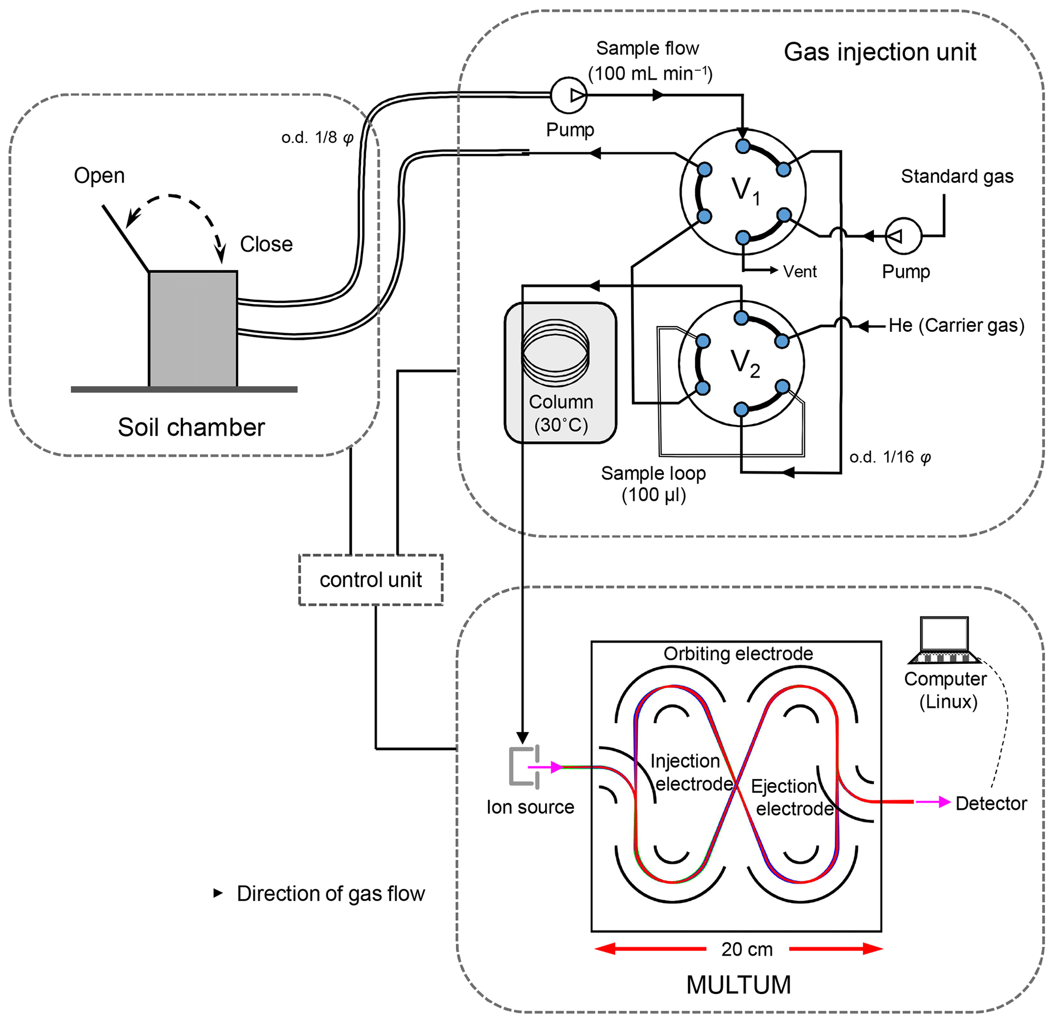
Figure 1Schematic of developed mass spectrometric multiple soil-gas flux measurement system with a portable high-resolution multi-turn time-of-flight mass spectrometer (MULTUM) coupled with an automated soil-gas flux chamber. The headspace gas in the chamber continuously circulates a sample loop in the gas injection unit through stainless-steel tubing. In each gas analysis, the headspace gas in the sample loop is injected into a capillary column for rough gas separation before analyzing each gas with MULTUM. (o.d. indicates outer diameter; ss indicates stainless steel).
The soil gas in the chamber headspace is continuously circulated through stainless-steel tubing ( m, outer diameter multiplied by length) between the chamber and the sample injection unit via an air pump (CM-15-12, Enomoto Micro Pump, Tokyo, Japan). The circulating soil gas continuously passes through a 100 µL sample loop (SL100CM, Valco Instruments, Houston, TX, USA) fitted to a port with a six-port auto valve (V1) (SAV-VA-11-65, FLOM, Tokyo, Japan). When the collected sample gas is analyzed with MULTUM (infiTOF-UHV, MSI Tokyo, Tokyo, Japan), the valve rotates and the soil-gas sample is injected into a porous-layer open tubular capillary column with a monolithic carbon layer (10 m×0.320 mm, length multiplied by inner diameter, 3.0 µM; GS-Carbon PLOT, Agilent Technologies, Santa Clara, CA, USA) with a carrier He gas stream (2.5 mL min−1) for rough gas separation before feeding into MULTUM. Another six-port auto valve (V2) (SAV-VA-11-65, FLOM, Tokyo, Japan) switches soil-gas sampling and standard gas injection for calibration. Sample gas injection occurs every 2.5 min, and both the sample and standard gas injections are controlled by the FPGA.
Although MULTUM has sufficient mass-resolving power for completely separating and ion peaks, we include the column to provide slight time lags between N2∕O2, CO2, and NO2 before injection into the system to improve quantification. In fact, omitting the separation in the time domain (20–60 s) causes several intrinsic MS problems. For example, the is derived directly from coexisting N2 and O2 at the electron impact (EI) source reaction. Further, the ionization of atmospheric trace gases with the main components of the atmosphere (e.g., N2, O2) restricts the ionization of coexisting trace gases in the ion source (ion-source saturation), which considerably worsens the detection limit of the trace gases. Finally, the dynamic ranges of the ion detector and signal acquisition are limited to 2–3 orders of magnitude, thereby impeding the simultaneous and accurate measurement of NO2 and CO2 within a single gas sample wherein the concentrations differ by more than 3 orders of magnitude. Thus, we adopt a hybrid ion detection and signal processing technique that selects either waveform averaging or ion counting to detect ions with intensities differing by 6 orders of magnitude (Kawai et al., 2018).
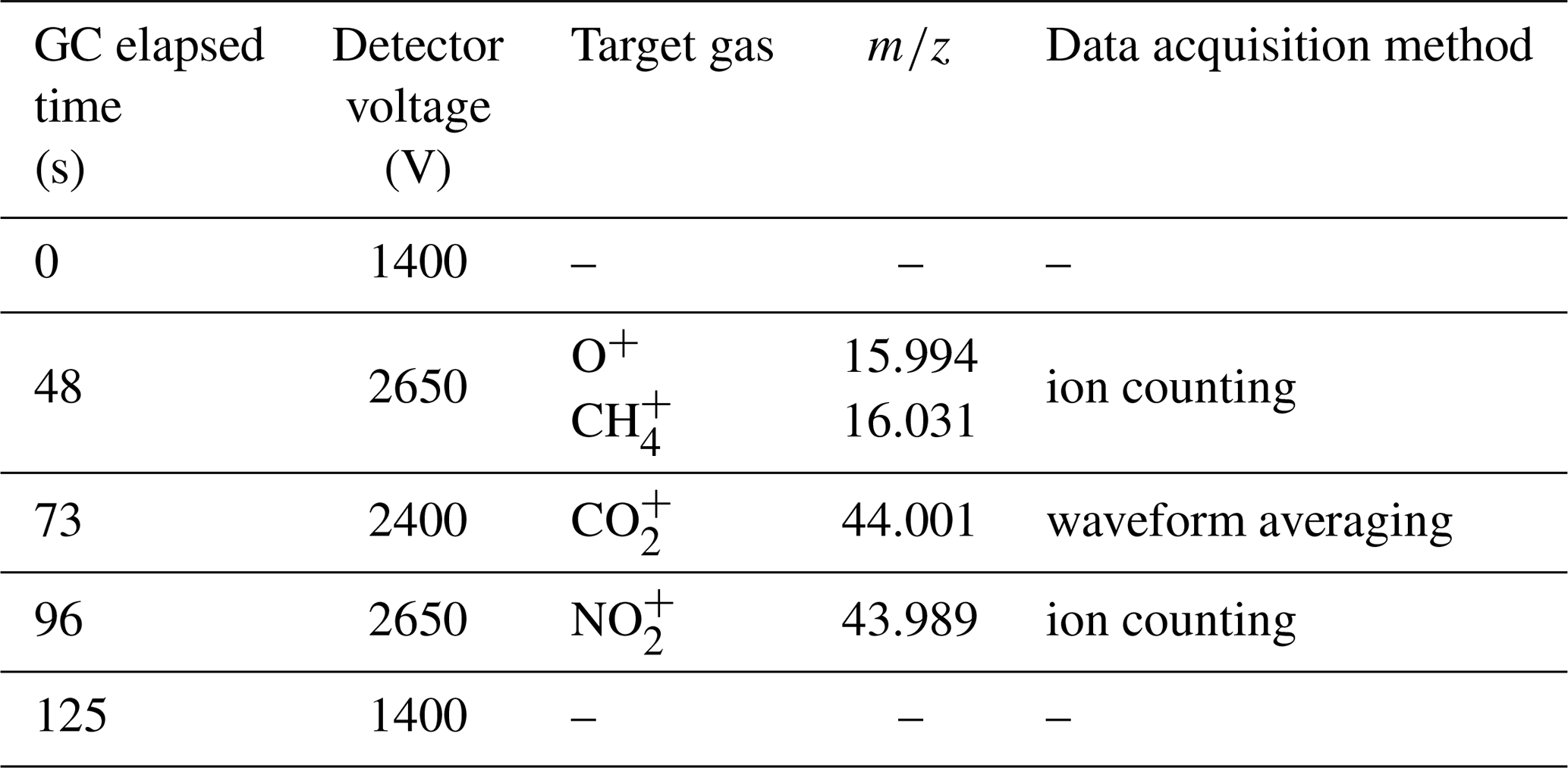
In the conventional waveform-averaging mode, it is difficult to recognize considerably less abundant ions (e.g., ) as an ion peak because such low-abundance ions are easily overwhelmed by background noise. In contrast, ion counting allows the detection of scarce ions (Hoffmann and Stoobant, 2007) by regarding ion peaks above a predefined threshold intensity (−10 mV in this study) as a single ion. However, counting loss occurs for abundant ions when two or more ions arrive at the detector within the minimum time resolution of the ion signal detection system. The present hybrid ion detection and signal processing scheme employs two detection modes using a single ion detector and recording system by selecting either waveform averaging or ion counting depending on the type of gas (at different periods from sample injection into the column) by changing the ion detector gain and real-time signal processing protocol (Hondo et al., 2017). Thus, a column is required to create small temporal separations for the detection of target ions and to select the appropriate measurement mode in addition to averting ion-source saturation. For the detection of , the ion detector voltage is set to 2400 V, and the conventional waveform recording and averaging are conducted for the time-of-flight ion signal where the voltage is set to 2650 V for the detection of O+, , and ; the real-time software thresholding (i.e., ion counting) is conducted for the acquired signal (Fig. 2). Though determination of oxygen concentration would be more accurate using detection, oxygen was detected as O+ (not as ) using the ion-counting mode because O+ (m∕z 15.99) can be simultaneously detected along with (m∕z 16.03). If oxygen is observed as (m∕z 32.00), another mass segment around m∕z 32.00 needs to be analyzed, and less measurement time can be allocated for and measurements, which results in lower sensitivity for and measurements. The optimized high-voltage settings of MULTUM for this study are listed in Table 1.
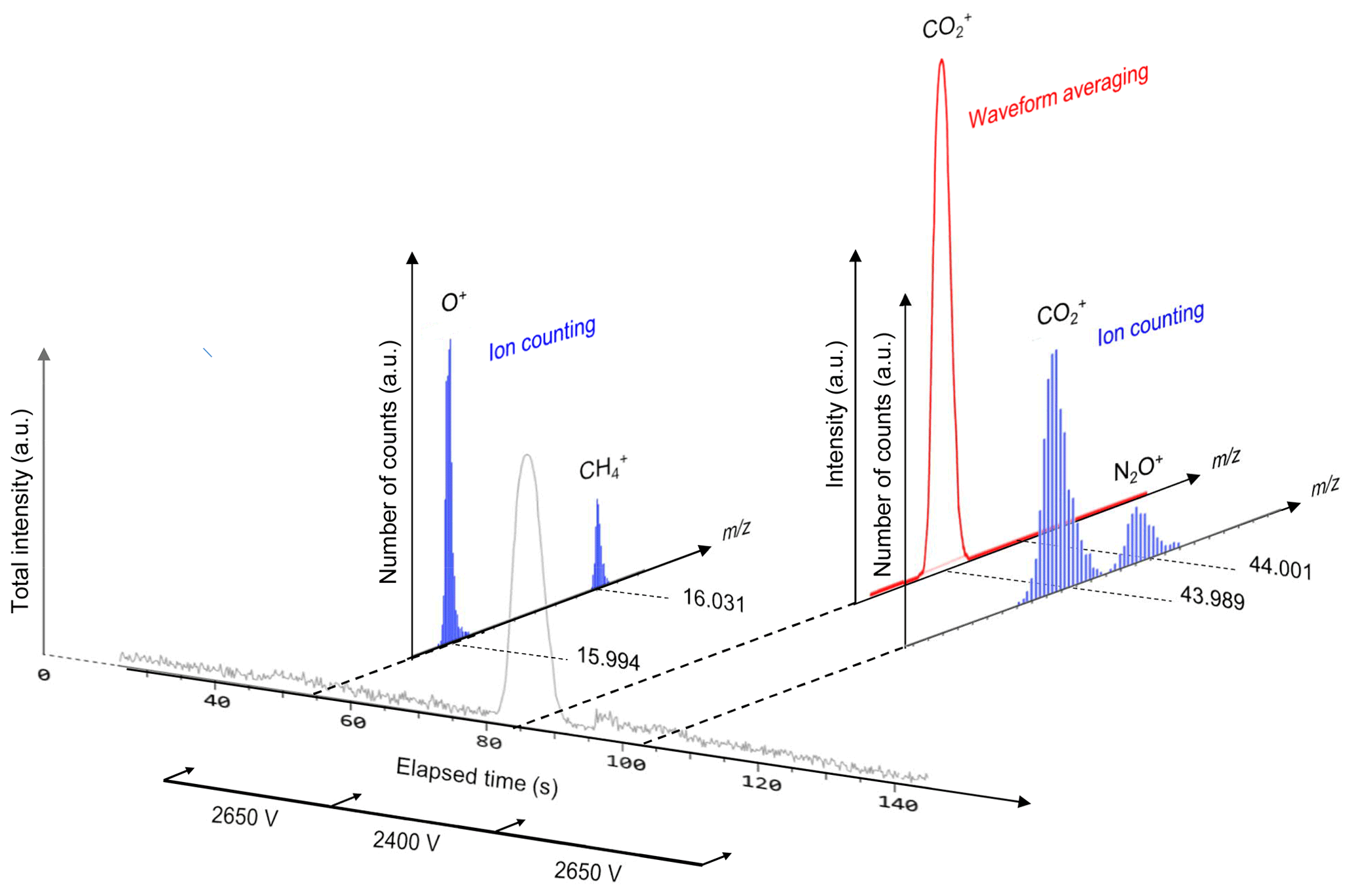
Figure 2Schematic of two-dimensional gas–ion separation for O2, CH4, CO2, and NO2 in chromatographic and m∕z domains using a short column for rough separation and high-resolution mass spectrometry (MULTUM) for further complete separation. O2, CH4, and NO2 are detected as O+, , and with ion-counting mode, whereas CO2 is detected as with waveform-averaging mode. In the chromatographic domain, CO2 and NO2 are not fully separated; however, in the m∕z domain, residual contributions of and are fully separated by high mass-resolving power of MULTUM.
Table 1Elapsed time between sample injection and corresponding adjustment of ion detector voltage in MULTUM to perform hybrid ion detection and signal processing (waveform averaging or ion counting) for specific target ions.
The gases injected into MULTUM are ionized by electron ionization at an electron acceleration voltage of 30 V, and the produced ions are mass analyzed at a repetition rate of 1 kHz with 30 laps of circular ion flight; this yields a mass resolution of approximately 10 000. After 30 laps, each ion is detected by an electron multiplier (ETP secondary electron multiplier 14882, ETP Ion Detect, Sydney, Australia). The ion signal from the ion detector is then amplified through a high-speed preamplifier (ORTEC 9301, Advanced Measurement Technology, Oak Ridge, TN, USA) and recorded and processed in real time with a high-speed 1 GS s−1 digitizer (U5303a, Keysight Technologies, Santa Rosa, CA, USA). Mass spectra are then transferred to a host PC (dual Intel eight-core/16-thread Xeon processor PC with Linux Debian 9.9 operating system). The data acquisition system is controlled by the QtPlatz open-source software (https://github.com/qtplatz, last access: 10 October 2019) with its plugin developed for the infiTOF system (Hondo et al., 2017; Jensen et al., 2017).
We calibrate the system with six different concentrations including blank gas (ultrapure N2), which are prepared from mixed standard gases (mixture of NO2, CH4, and CO2) and O2 standard gas by diluting with ultrapure N2 (>99.9995 %; Takachiho Chemical Industrial, Tokyo, Japan). We use two certified standard gases (standard no. 1: NO2, 279 ppbv; CH4, 1.47 ppmv; CO2, 421 ppmv in N2; standard no. 2: NO2, 1752 ppbv; CH4, 2.97 ppmv; CO2, 1705 ppmv in N2; Sumitomo Seika Chemicals, Osaka, Japan) and O2 standard gas (20.9 % in N2 balance gas; Takachiho Chemical Industrial, Tokyo, Japan). The gas mixing rates are adjusted using mass flow controllers (model 8500 series, KOFLOC, Kojima Instruments, Kyoto, Japan) calibrated using a soap film flowmeter (HORIBA STEC, Kyoto, Japan).
We continuously measured the standard gases using the developed MULTUM–soil chamber system and estimated the detection limits for NO2, CO2, CH4, and O2 based on the IUPAC criteria (Long and Winefordner, 1983) given as
where k is a constant that determines the confidence level (we set k=3 for a confidence level above 99 %), RSD is the standard deviation of the ion count or peak area of the target gas when measuring ultrapure N2, and m is the slope of linear regression obtained from the measurement of the six abovementioned gas concentrations prepared from the standard gases and ultrapure N2 based on 10 replicate measurements of each gas.
2.2 Flux measurement using MULTUM–soil chamber system
The fluxes of target soil gases are determined from the variation in the target gas concentration while the chamber is closed. During each flux measurement, nine consecutive measurements are conducted over 20 min. A complete flux measurement is performed once per hour. The chamber is closed during the first 20 min of the flux measurement, and it remains open during the remaining 40 min. Standard no. 2 and atmospheric air measurements are conducted to monitor the MULTUM stability (Fig. 3). The standard gas measurement is repeated five times and atmospheric air measurement is repeated 10 times when the chamber is open. The fluxes of observed soil gases are calculated as (Minamikawa et al., 2015)
where ΔC∕Δt is the concentration variation of the target gas (ppbv NO2, ppmv CH4, or ppmv CO2 h−1) during the flux measurement period, V is the chamber volume (m3), A is the chamber area (m2), ρ is the gas density (kg m−3), T is mean air temperature inside the chamber (∘C), and α is a conversion factor to transform NO2 into N, and CH4, CO2 into C. We determine ΔC∕Δt by applying linear regression to the data obtained from the nine consecutive concentration measurements when the chamber is closed.
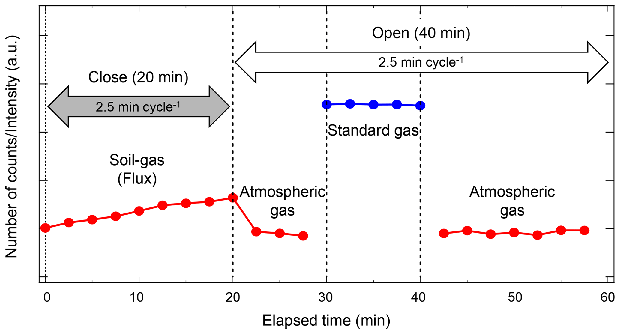
Figure 3Example sequence of flux measurement conducted over 1 h and continued during field and laboratory flux observations. The flux chamber is closed for the first 20 min of flux measurement. During the remaining 40 min, the chamber is open and standard and atmospheric gas measurements are conducted for system stability verification and calibration.
Besides the flux measurement, we monitor soil temperatures and moisture with a portable digital thermometer (EM50 Data Logger, METER Group, Pullman, WA, USA). Further, we monitor the air temperature inside the chamber and the ambient temperature using a temperature data logger (Thermo Recorder TR-52i, T&D Corporation, Nagano, Japan).
The minimum detectable flux (MDF) of each soil gas can be estimated based on the derivations by Courtois et al. (2019) originally developed by Christiansen et al. (2015) and Nickerson (2016) as
where Aa, i is the analytical accuracy of MULTUM for gas i, tc is the closure time of the soil flux chamber per flux measurement (20 min), n is the number of gas concentration measurements to calculate the gas flux (i.e., nine measurements), V is the volume of the flux chamber (0.018 m3), P is the atmospheric pressure in kPa, S is the inner surface area of the flux chamber (0.049 m2), R is the ideal gas constant (8.314 m3 Pa K−1 mol−1), and T is the ambient temperature surrounding the chamber in K.
The MDF metric is a common performance metric in flux measurements; in particular, it is used in flux measurement methods based on continuous gas concentration observation with the chamber technique. Because MDF is a useful metric for comparing results between the cavity ring-down spectroscopy (CRDS) and our MS-based instrument, we employed the MDF for the comparison. The device accuracy (Aa, i) is defined as the measurement accuracy of an instrument (Christiansen et al., 2015; Nickerson, 2016). In the flux measurement with the CRDS instrument, they used the accuracy value provided by the manufacturer. For our system, we define the analytical accuracy (Aa, i) as the analytical precision (measurement uncertainty) of MULTUM for gas i and use 2 standard deviations (2σ) obtained from 994 measurements of the gas in air. However, we found that the MDF was not a proper metric for our flux measurement and thus defined new metrics – minimum quantitative flux (MQF) – for better assessment of the reliability. Since flux is the rate of increase or decrease in the gas concentration of interest in the closed chamber, we determine the flux by applying linear regression to every set of the nine consecutive gas concentration measurements in the closed chamber period over 20 min. We noticed that the quality of the linear regression analysis was quite poor even when the flux values were above MDF and the determined flux values were not reliable enough for further scientific discussion. We thus additionally evaluated the MQFs for each gas species to examine quantitatively reliable fluxes in our study. The MQF is determined from the precision of the slopes (rates of gas concentration changes) in the flux measurement relative to the true slope. However, the true slopes are difficult to determine in actual field measurements, and therefore we conducted a simulation study to characterize the MQF of the current instrument for each gas species.
We first defined a “true” flux value of the gas for the model simulation assuming that the flux remained constant when the chamber is closed. Based on the defined true flux value and chamber dimension, true gas concentrations to be measured in the chamber were calculated over time when the chamber was closed. To simulate a realistic observation, a random measurement error based on the standard deviation derived from the atmospheric gas measurements was intentionally added to the predefined true gas concentrations when the chamber was closed. The simulated nine consecutive observation data were then used for flux determination with linear regression analysis, whose results were further characterized for MQF estimation. For each defined flux value, 10 000 sets of flux measurements were simulated, 10 000 corresponding slopes were obtained, and the standard deviations of the slopes were characterized. The simulation was conducted on a scientific graphical data processing software (Igor Pro, WaveMetrics, Lake Oswego, OR, USA) and the random measurement error was generated with a built-in Gaussian distribution noise generator.
2.3 Laboratory tests
We conducted laboratory flux measurement tests of NO2, CH4, CO2, and O2 using a soil sample collected at the university farm of Ehime University. The soil was collected from 0 to 10 cm below the soil surface. After sampling, the soil was sieved to remove roots and stones. A urea solution (CO(NH2)2) was added to the soil (4 g of urea to 1 kg of soil) to promote NO2 production. Then, the soil was air dried for a few days prior to flux measurement. The soil was spread in a 6 L plastic container, and the automated flux chamber was placed on the soil. The flux measurement cycle was the same as that used for the field observation shown in Fig. 3 (chamber is closed for 20 min, flux measurement with nine concentration measurements occurs every 2.5 min, and chamber is open for the remaining 40 min). When the chamber was open, the standard gas and atmospheric air measurements were conducted for system calibration and verification. After 22 h from the start of the laboratory flux measurement, 3 L of water were sprayed on the soil for initiating the production or consumption of CO2, CH4, and NO2, and the flux measurement proceeded for 46 h.
2.4 Field observations
We deployed the developed MULTUM–soil chamber system at the university farm of Ehime University (Matsuyama-shi, Ehime, Japan) for a field observation over 5 d (3–8 September 2018). The university farm is used for various agricultural production and soil studies (Toma, et al., 2019; Asagi and Ueno, 2009).
The automated flux chamber was placed on a ridge in the upland field, as shown in the left panel of Fig. 4. The field test was conducted during the fallow period (i.e., bare field condition). The soil pH, electric conductivity, and texture were 5.3, 34.0 µS cm−1, and sandy loam (sand, 75.6 %; silt, 10.6 %; clay, 13.8 %), respectively. On 2 September, ammonium sulfate (150 kg N ha−1) and dried cattle feces (10 Mg ha−1 of fresh weight) were added and incorporated into the soil surface (0–15 cm depth). After plowing, the soil bulk density and porosity were 1.02 g cm−3 and 62.9 %, respectively. The automated soil chamber was installed immediately after incorporation. The total carbon (C) and nitrogen (N) content of the dried cattle feces was 36.1 % and 2.08 %, respectively. The other components of the MULTUM–soil chamber system (i.e., MULTUM platform, control, and data acquisition system) were installed at a nearby goat hut that had a room temperature of 27±2 ∘C. Two 5 m long stainless-steel tubes (1∕8 inch outer diameter) were used to connect the chamber and the six-port auto valve in the gas injection unit to circulate headspace gas within the chamber.
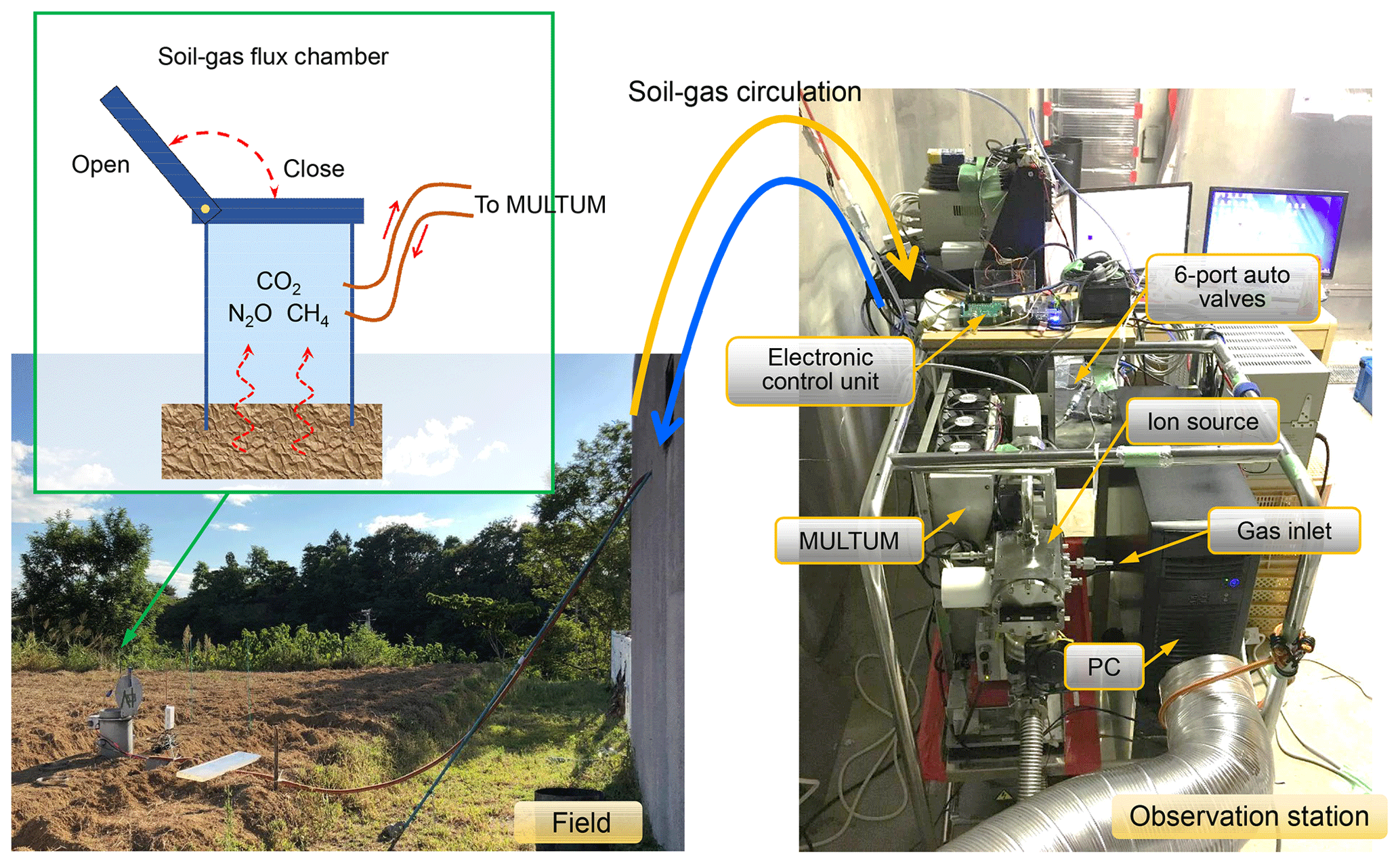
Figure 4Instrument setup during a field flux campaign at the university farm of Ehime University (Matsuyama-shi, Ehime, Japan).
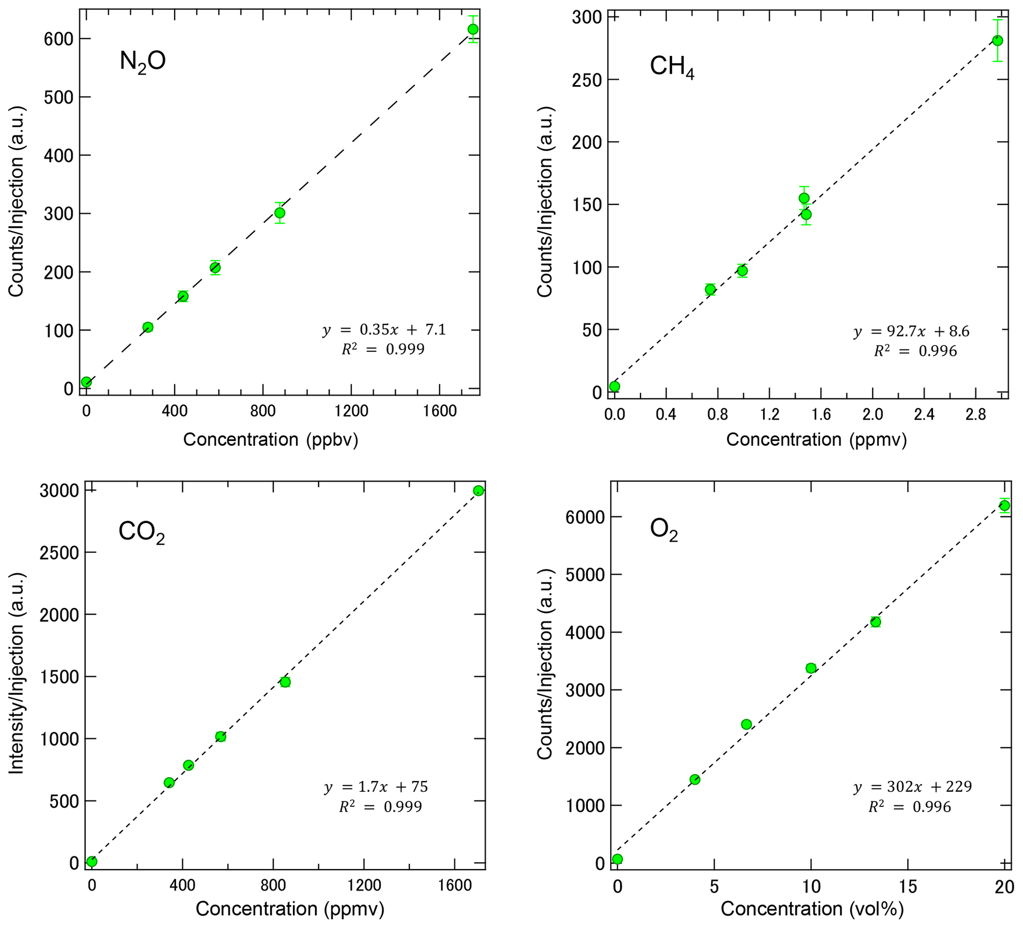
Figure 5Calibration curves of MULTUM obtained by introducing standard gases of NO2, CH4, CO2, and O2 diluted by ultrapure N2. The coefficients of determination (R2) for each linear regression were above 0.996 for all gases regardless of the huge concentration difference of 6 orders of magnitude. Each point was based on 10 replicate injections.
3.1 Laboratory characterization of MULTUM–soil chamber system performance
In the laboratory, we characterized the performance of the developed MULTUM–soil chamber system by introducing standard gases through the gas injection unit at six different concentrations and by following the procedure for field observations. As shown in Fig. 5, MULTUM linearly responds to the gas concentrations during measurement, thereby obtaining coefficients of determination (R2) for all linear regression results above 0.996. Blank concentrations checked by introducing ultrapure N2 were very small compared to the atmospheric concentrations of the target gases. The calculated detection limits were 12 ppbv for NO2; 50 ppbv, CH4; 13 ppmv, CO2; and 0.68 vol %, O2, based on Eq. (2).
To verify the stability of the developed MULTUM–soil chamber system, we conducted continuous measurements of atmospheric NO2, CH4, CO2, and O2 in the laboratory with the flux chamber open (Fig. 6). The set of NO2, CH4, CO2, and O2 measurements was repeated every 2.5 min over 42 h. In the laboratory, the room temperature was maintained at 23±1 ∘C and the relative humidity was around 15 % at the beginning of the measurement; it increased to 30 %–33 % after the midnight of 31 January 2019. The atmospheric pressure during the laboratory measurement period ranged between 1005 and 1014 hPa. The variations of atmospheric NO2, CH4, CO2, and O2 measurements are shown as histograms in Fig. 7. Because the distributions agree with Gaussian distributions plotted as dashed lines in Fig. 7, we calculated the standard deviations (2σ) of each gas from the measurements to obtain Aa, i. The Aa, i obtained from the atmospheric air measurements were 22 ppbv for NO2; 102 ppbv, CH4; 8.1 ppmv, CO2; and 0.38 vol %, O2. These variations may be subject to the natural variabilities of atmospheric concentrations; however, we consider that they are instrumental variations because their distributions demonstrated good agreement with Gaussian distributions (Fig. 7) and the analytical precision obtained from the measurements of standard no. 1 and O2 standard in the laboratory (±34 ppbv for NO2; ±170 ppbv, CH4; ±16 ppmv, CO2; and ±0.60 vol %, O2, 2σ) almost corresponded to those obtained from atmospheric air. Using the standard gas rather than ambient air usually yields better instrumental performance because ambient air contains considerably more complicated gas species including water vapor, which can affect the precision of mass spectrometric measurement. Our final goal in our instrumental development is to construct a new instrument for field observation; soil-gas flux is determined from the change in gas concentration in the flux chamber relative to its atmospheric concentration. Thus, we considered that using ambient air measurement for our instrumental performance test is more appropriate and practical for our research purpose.
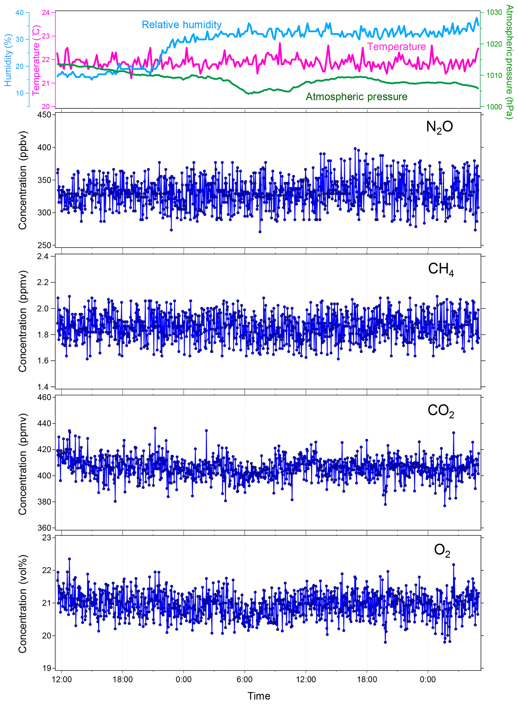
Figure 6Continuous measurements of atmospheric NO2, CH4, CO2, and O2 in the laboratory with the soil chamber opened. Every 2.5 min, concentrations of the four gases were observed. The blue dots indicate individual data points. The top panel shows the variations of atmospheric conditions during the laboratory measurement: atmospheric temperature (∘C), pressure (hPa), and relative humidity (%).

Figure 7Frequency distributions of measured atmospheric concentrations of NO2, CH4, CO2, and O2 (994 measurements) during the laboratory measurement with the MULTUM-soil chamber system. For visual comparison, Gaussian distributions are plotted as dotted lines. The average (avg) and standard deviation (SD) shown in the panels were calculated from the atmospheric measurement for each gas species.
3.2 Laboratory flux measurement test
Before the field campaign, we conducted a laboratory flux measurement test to confirm whether our newly developed instrument could capture each soil-gas flux when water was added, which is a major fluctuation factor of soil-gas flux. The temporal variations of the measured gas concentrations when the chamber is closed is shown in Fig. 8. Only data acquired when the chamber is closed (flux measurement periods) are depicted for simplification; however, the system stability verification and calibration were conducted when the chamber was open. At 22 h, water (approximately 3 L) was sprayed on the soil surface as environmental perturbation resembling rainfall to reactivate the dormant soil biological processes. Immediately after water addition, the emission of NO2 and CO2 began to change in different ways. For example, the CO2 emission rapidly increased and reached its maximum 2 h after water addition and remained relatively high, whereas NO2 emission gradually increased until 20 h after water addition at a seemingly constant rate.

Figure 8Example of continuous and simultaneous flux measurement of NO2, CH4, CO2, and O2 in the laboratory with a simulated plowed field. After 22 h, water (3 L) was sprayed on the soil surface. Immediately after the water addition, emission of NO2 and CO2 began to change in different ways. For CH4 and O2, no flux beyond their minimum quantitative fluxes was observed throughout the flux measurement.
Such increases in soil CO2 flux by rainfall or rewetting soil have been reported previously (Lee et al., 2002; Smith and Owens, 2010; Gelfand et al., 2015; Kostyanovsky et al., 2019); they enhance microbial activity and population and boost the availability of carbon and nutrients because of either rewetting or the assemblages (Fierer and Schimel, 2003; Iovieno and Bååth, 2008; Blazewicz et al., 2014). A similar increase in NO2 flux on rewetting soil has been reported (Nobre et al., 2001; Dobbie and Smith, 2003; Smith and Owens, 2010; Gelfand et al., 2015; Schwenke and Haigh, 2016; Leitner et al., 2017; Barba et al., 2019; Kostyanovsky et al., 2019), although very few papers reported the simultaneous response of NO2 and CO2 fluxes upon artificial watering (Smith and Owens, 2010; Gelfand et al., 2015; Kostyanovsky et al., 2019). Only Kostyanovsky et al. (2019) reported short-term flux changes of both CO2 and NO2 upon simulated rainfall with a time resolution of 2 h. They showed that the simulated rainfall immediately triggered increases in both CO2 and NO2 fluxes; however, the increase in CO2 flux continued until about 3 h after the simulated rainfall, while that in NO2 flux continued until about 5 h after the simulated rainfall. In the present laboratory test, CO2 and NO2 fluxes showed different temporal behavior from that observed by Kostyanovsky et al. (2019), although the observed NO2 flux change was similar to that observed by Leitner et al. (2017). We speculate that the slow increase in NO2 flux may reflect a slow buildup of nitrification and denitrification microorganisms after watering, although further studies that consider both the biological and physicochemical aspects of the soil-gas formations are necessary for gaining better understanding. The fluxes of CH4 and O2 during the laboratory test were below their MDFs.
3.3 Minimum detectable and minimum quantitative fluxes of GHGs and O2
In Fig. 7, the frequencies of atmospheric concentrations of NO2, CH4, CO2, and O2 observed with the MULTUM–soil chamber system during the laboratory stability check (Fig. 6) are compiled as histograms. Their frequency distributions agree well with Gaussian distributions (plotted as dashed lines in Fig. 7), and thus their standard deviations are considered to have the Aa, i of the MULTUM–soil chamber system for each gas. The Aa, i is defined as the analytical accuracy (measurement uncertainty) of MULTUM for gas i and the use of 2 standard deviations (2σ) obtained from 994 measurements of atmospheric gas as a reference.
We estimated the MDFs based on Eq. (3) using the Aa, i for each gas, and we obtained 17.2 , 35.4 , 2.6 mg C m−2 h−1, and 2.9 g O2 m−2 h−1 for NO2, CH4, CO2, and O2, respectively. However, the MDF is not a practical measure for the reliable quantification of flux. Thus, we evaluated the MQF for each gas as the quantitatively reliable flux in our study via model simulation.
Figure 9a–d show the relationship between the true flux and the calculated fluxes from the simulation. The error bars in the figures represent error ranges of fluxes (2σ) determined from the simulation. The average fluxes determined by the simulation were almost equal to their corresponding true fluxes, and the errors were relatively constant. Here, we define MQF as the flux when the true flux is equal to the error (2σ) of the corresponding simulated flux. We obtained the MQFs of 70.2 for NO2; 139 , CH4; 11.7 mg C m−2 h−1, CO2; and 9.8 g O2 m−2 h−1, O2. We consider the observed fluxes below the MQFs as qualitatively uncertain, and we do not use them in subsequent data analyses for this study.

Figure 9Relationship between true and simulated fluxes of (a) NO2, (b) CH4, (c) CO2, and (d) O2. In the simulated flux determination, random deviations of each gas concentration measurements were considered. The error bars in the figures represent 2 standard deviations of the fluxes derived from 10 000 simulated flux measurements for each flux condition. The MQF is defined as a minimum quantitative flux when the true flux is equal to 2 standard deviations of simulated flux.
We conducted data quality checks for the filed observation flux data using coefficients of determination (R2) in the linear regression analysis for nine consecutive concentration measurements when the chamber was closed. Figure 10 shows the relationships between observed fluxes and the corresponding R2 in the NO2 and CO2 flux derivation during field flux observation at Ehime University. The R2 was approximately 0.4 at its MQF (70.2 ) in the NO2 flux observation. The data with R2=0.4 in their linear regression analysis are regarded to have a statistically significant correlation, which supports that MQF is a reasonable metric for reliable quantification. In the field NO2 flux measurement, R2 increased with an increase in the observed flux, which indicates that the improvement of quality in NO2 measurement (i.e., detection limit and sensitivity) is desirable for more reliable determination, and in particular, under a low NO2 flux condition. All CO2 flux measurements showed R2>0.9, indicating that the present system is reliable for CO2 flux determination. The observed fluxes of CH4 and O2 during the laboratory/field study were usually below their MDFs; however, during a different field campaign in March 2019 at the same field, the CH4 flux above the MDF was observed (Fig. 12). For O2 flux, the analytical precision for the current O2 concentration measurement was ±0.60 vol % (±6000 ppmv). The current flux observation was under a dark condition and the CO2 concentration change was caused by respiration of the soil organisms. Therefore, the increase in CO2 concentration in the flux chamber is roughly equal to the decrease in O2 concentration during flux measurement. As shown in Fig. 8, to capture the O2 flux, an analytical precision of more than 3 orders of magnitude is necessary because the CO2 concentration change is about 100 ppmv after water spraying. It is considerably difficult to achieve an improvement in measurement precision by more than 3 orders of magnitude. Although quantitative O2 flux measurement is difficult, our developed instrument can detect the variation in O2 concentration as a tracer for the redox state in soil environments (Kaiser et al., 2018).
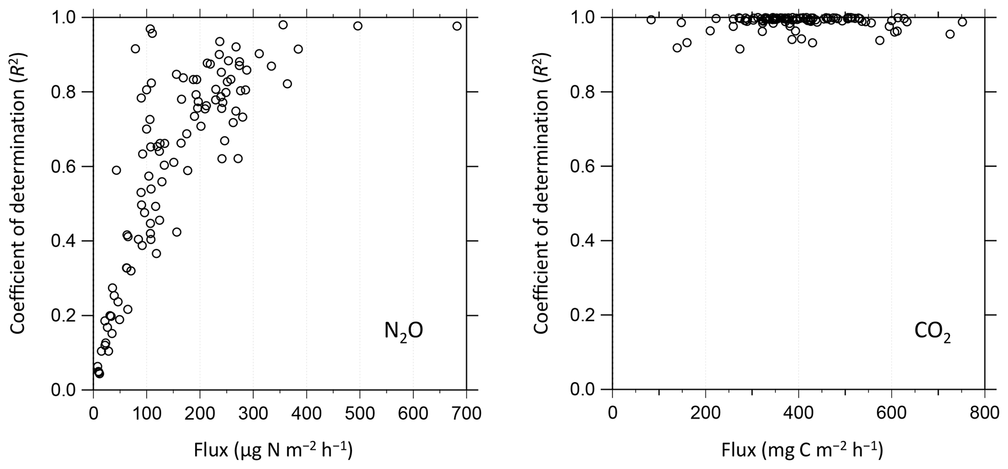
Figure 10Relationship between determined fluxes during field observation and coefficients of determination (R2) in the linear regression to derive corresponding slopes (fluxes) from nine consecutive gas concentration observations per flux measurement.
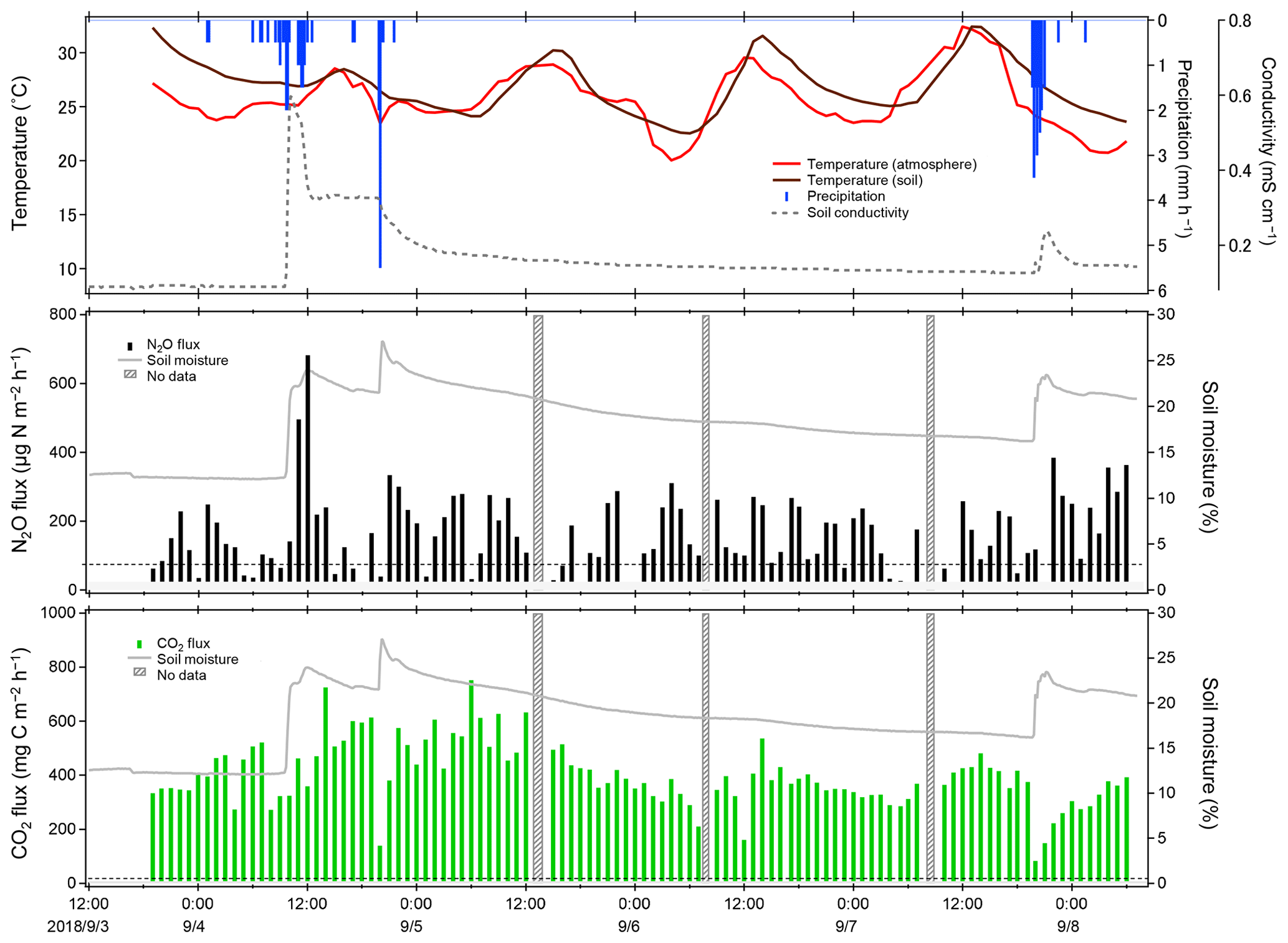
Figure 11Temporal variations of observed NO2 and CO2 fluxes at the university farm of Ehime University during field flux observation in September 2018. The dotted lines represent MQFs. Fluxes below the MDF are masked. The shaded areas represent no data due to measurement interruption by system issues, and so on.
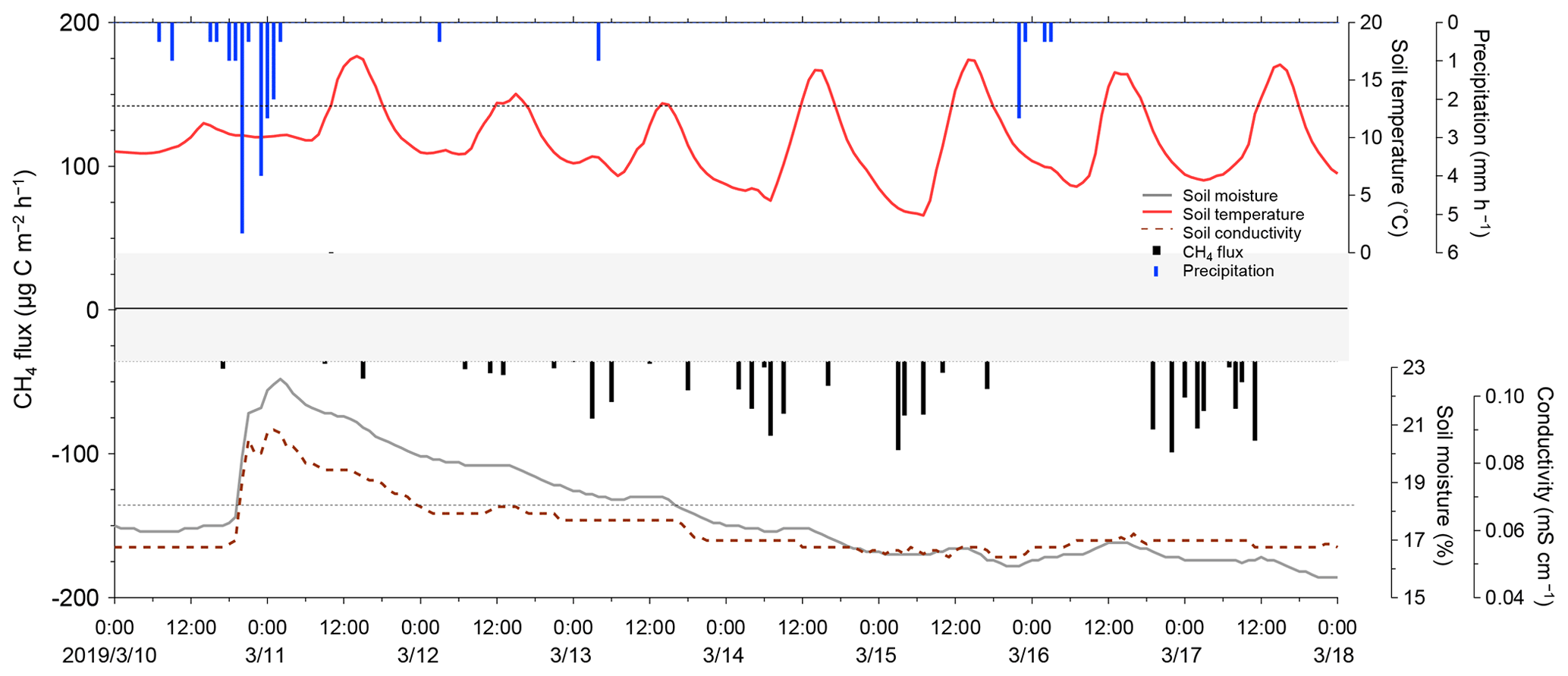
Figure 12Temporal variations of observed CH4 flux at the university farm of Ehime University during field flux observation in March 2019. Fluxes smaller than the MDF (35.4 ) are masked. Dotted grey lines represent the MQF (139 ).
3.4 Field observation
Temporal variations of climate, N2O, and CO2 fluxes are shown in Fig. 11. The NO2 fluxes were mostly below 300 and generally dependent on soil moisture, which substantially affected the production, consumption, and atmospheric exchange of GHGs (Davidson and Swank, 1986; Dobbie and Smith, 2003; Liebig et al., 2005; Ellert and Janzen, 2008; Sainju et al., 2012). An interesting event was observed in the NO2 flux on 4 September. The NO2 flux abruptly increased from 70 to 682 within a few hours after rainfall, while a gradually increase in CO2 flux was observed. These observed responses exhibit sharp contrast with our laboratory flux measurement test, in which CO2 flux showed a rapid increase, while NO2 flux showed a slow sustained increase upon water spraying (Fig. 8). Various studies have reported an increase in the NO2 flux after rainfall (Nobre et al., 2001; Dobbie and Smith, 2003; Smith and Owens, 2010; Gelfand et al., 2015; Schwenke and Haigh, 2016; Leitner et al., 2017; Barba et al., 2019; Kostyanovsky et al., 2019) and similar increases in CO2 flux after rainfall have also been reported (Lee et al., 2002; Smith and Owens, 2010; Gelfand et al., 2015; Kostyanovsky et al., 2019). However, no short-term responses of CO2 and NO2 fluxes similar to our observation upon rainfall have been reported. Further, two heavier rainfall events occurred on 5 and 7 September; however, the NO2 flux showed no obvious increase similar to that after the first rainfall. The different responses in NO2 flux may reflect the complexity in microbial and nutrient dynamics initiated in the soil upon rainfall (Gordon et al., 2008; Blazewicz et al., 2014), although further detailed studies that investigate both biological and physicochemical aspects of the soil-gas formations are necessary to determine the causes of the response. The CO2 flux, in contrast, remained constant except during rainfall periods, in which an abrupt decrease and quick recovery within several hours of the flux occurred. This can be attributed to the suppression of CO2 permeation within the soil column caused by a capping effect of wet soil and different vertical distributions within the soil column; although these explanations are feasible, they require further temporal and spatial investigation.
We developed a field-deployable MS-based multiple gas flux measurement system utilizing a portable high-resolution mass spectrometer (MULTUM) combined with an automated soil-gas chamber. The MULTUM was coupled with a short gas separation column to roughly separate atmospheric major and trace gases over a short period, and a new hybrid ion detection and signal processing technique was employed to ensure a much wider dynamic range for quantitative and simultaneous measurement of multiple gas concentrations that differ by 6 orders of magnitude. The present hourly continuous gas flux measurement of multiple gas species clearly indicates its considerable advantage of capturing rapid and different temporal responses of different gas species toward sporadic abrupt environmental changes (e.g., sudden rainfall), which provides more detailed understanding of underlying soil biological and physicochemical processes.
Further improvement in the detection limit and analytical precision is required for the accurate measurements of low GHG fluxes, in particular, for NO2 and CH4. We believe that the improvement in the sensitivity by 1 order of magnitude can be achieved relatively easily by retrofitting a larger vacuum pump to the MULTUM (from 50 to 250 L s−1), using a higher mass measurement rate (from current 1 to 10 kHz), and using a flux chamber with a lower ratio of the height to bottom area. The privilege of MS-based gas measurement in highly sensitive and wider range of detectable gas species, including reactive-nitrogen gases (e.g., NO, NO2), noble gases (e.g., Ar, Ne), inorganic gases (e.g., N2, H2, CO, H2S), and small organic gases (e.g., ethylene) should be quite advantageous in providing deeper insights into soil microbiological ecosystems, physicochemical processes, and their responses to environmental perturbations. A wide variety of gas species such as He, Ar, and polychlorinated biphenyls have already applied by MULTUM (Jense et al., 2017; Kawai et al., 2018; Shimma et al., 2013). Coupling proton transfer reaction (PTR) ionization source with the MULTUM can help detect a wider range of individual BVOCs and subsequently their soil–atmosphere fluxes, and our group is coupling a PTR ion source to MULTUM.
We expect that further instrumental improvements and further expansion in detectable gas species will boost providing deeper insights on the biological and physicochemical processes in soil and lead to more comprehensive understanding.
Data are available upon request.
NN led this research project and conducted a major part of the study. YT coordinated the field campaign, assisted with the field flux measurement, and provided valuable feedback and advice for the field measurements. YI assisted in conducting a field test. TH constructed the hybrid ion detection and signal processing technique as well as the data analysis tools. HF developed a prototype of the multiple gas measurement (MULTUM) system. RH and MT created the conceptual framework of this study. All authors discussed the results and contributed to the preparation of the final manuscript.
The authors declare that they have no conflict of interest.
We thank the supporting staff at the university farm in Ehime University for their assistance during the field observation. Further, we thank Hisanori Matsuoka for his assistance in developing and optimizing the electrical systems, and Toshio Ichihara for the fabrication of the soil chamber. We would also like to thank the anonymous reviewers for their comments and suggestions that helped improve this paper.
This research has been supported by JSPS Challenging Research (Exploratory) (grant no. 17K20044).
This paper was edited by Christian Brümmer and reviewed by two anonymous referees.
Anan, T., Shimma, S., Toma, Y., Hashidoko, Y., Hatano, R., and Toyoda, M.: Real time monitoring of gases emitted from soils using a multiturn time-of-flight mass spectrometer “MULTUM-S II”, Environ. Sci: Proc. Imp., 16, 2752–2757, https://doi.org/10.1039/C4EM00339J, 2014.
Arias-Navarro, C., Díaz-Pinés, E., Klatt, S., Brandt, P., Rufino, M. C., Butterbach-Bahl, K., and Verchot, L. V.: Spatial variability of soil NO2 and CO2 fluxes in different topographic positions in a tropical mountain forest in Kenya, J. Geophys. Res. Biogeosci., 122, 514–527, https://doi.org/10.1002/2016JG003667, 2017.
Asagi, N. and Ueno, H.: Nitrogen dynamics in paddy soil applied with various 15N-labelled green manures, Plant Soil, 322, 251–262, https://doi.org/10.1007/s11104-009-9913-4, 2009.
Barba, J., Poyatos, R., and Vargas, R.: Automated measurements of greenhouse gases fluxes from tree stems and soils: magnitudes, patterns and drivers, Sci. Rep., 9, 1–13, https://doi.org/10.1038/s41598-019-39663-8, 2019.
Blazewicz, S. J., Schwartz, E., and Firestone, M. K.: Growth and death of bacteria and fungi underlie rainfall-induced carbon dioxide pulses from seasonally dried soil, Ecology, 95, 1162-1172, https://doi.org/10.1890/13-1031.1, 2014.
Brannon, E. Q., Moseman-Valtierra, S. M., Rella, C. W., Martin, R. M., Chen, X., and Tang, J.: Evaluation of laser-based spectrometers for greenhouse gas flux measurements in coastal marshes, Limnol. Oceanogr. Meth., 14, 466–476, https://doi.org/10.1002/lom3.10105, 2016.
Christiansen, J. R., Outhwaite, J., and Smukler, S. M.: Comparison of CO2, CH4 and NO2 soil-atmosphere exchange measured in static chambers with cavity ring-down spectroscopy and gas chromatography, Agric. For. Meteorol., 211–212, 48–57, https://doi.org/10.1016/j.agrformet.2015.06.004, 2015.
Courtois, E. A., Stahl, C., Burban, B., Van den Berge, J., Berveiller, D., Bréchet, L., Soong, J. L., Arriga, N., Peñuelas, J., and Janssens, I. A.: Automatic high-frequency measurements of full soil greenhouse gas fluxes in a tropical forest, Biogeosciences, 16, 785–796, https://doi.org/10.5194/bg-16-785-2019, 2019.
Davidson, E. A. and Swank, W. T.: Environmental parameters regulating gaseous nitrogen losses from two forested ecosystems via nitrification and denitrification, Appl. Environ. Microbiol., 52, 1287–1292, PMID: 16347234, PMCID: PMC239223, 1986.
Dick, L, Skiba, U., and Wilson, L.: The effect of rainfall on NO and NO2 emissions from Ugandan agroforest soils, Phyton-Annales Rei Botanicae, 41, 73–80, 2001.
Dobbie, K. E. and Smith, K. A.: Nitrous oxide emission factors for agricultural soils in Great Britain: the impact of soil water-filled pore space and other controlling variables, Glob. Change Biol., 9, 204–218, https://doi.org/10.1046/j.1365-2486.2003.00563.x, 2003.
Ellert, B. H. and Janzen, H. H.: Nitrous oxide, carbon dioxide and methane emissions from irrigated cropping systems as in?uenced by legumes, manure and fertilizer. Can. J. Soil Sci., 88, 207–217, https://doi.org/10.4141/CJSS06036, 2008.
Fierer, N. and Schimel, J. P.: A proposed mechanism for the pulse in carbon dioxide production commonly observed following the rapid rewetting of a dry soil, Soil Sci. Soc. Am. J., 67, 798–805, https://doi.org/10.2136/sssaj2003.0798, 2013.
Gelfand, I., Cui, M., Tang, J., and Robertson, G. P.: Short-term drought response of NO2 and CO2 emissions from mesic agricultural soils in the US Midwest, Agric. Ecosyst. Environ., 212, 127–133, https://doi.org/10.1016/j.agee.2015.07.005, 2015.
Gordon, H., Haygarth, P. M., and Bardgett, R. D.: Drying and rewetting effects on soil microbial community composition and nutrient leaching, Soil Biol. Biochem., 40, 302–311, https://doi.org/10.1007/s00248-010-9723-5, 2008.
Hall, S. J., McDowell, W. H., and Silver, W. L.: When Wet Gets Wetter: Decoupling of moisture, redox biogeochemistry, and greenhouse gas fluxes in a humid tropical forest soil, Ecosystems, 16, 576–589, https://doi.org/10.1007/s10021-012-9631-2, 2013.
Heil, J., Vereecken, H., and Brüggemann, N.: A review of chemical reactions of nitrification intermediates and their role in nitrogen cycling and nitrogen trace gas formation in soil. Eur. J. Soil Sci., 67, 23–39, https://doi.org/10.1111/ejss.12306, 2016.
Hoffmann, E. and Stroobant, V.: Mass Spectrometry Principles and Applications, 3rd edition, Wiley, Chichester, England, 2007.
Hondo, T., Jensen, K. R., Aoki, J., and Toyoda, M.: A new approach for accurate mass assignment on a multi-turn time-of-flight mass spectrometer, Eur. J. Mass Spectrom., 23, 385–392, https://doi.org/10.1177/1469066717723755, 2017.
Huang, J., Huang, J., Liu, X., Li, C., Ding, L., and Yu, H.: The global oxygen budget and its future projection, Sci. Bull., 63, 1180–1186, https://doi.org/10.1016/j.scib.2018.07.023, 2018.
Insam, H., and Seewald, M. S.: Volatile organic compounds (VOCs) in soils, Biol. Fert. Soils, 46, 199–213, https://doi.org/10.1007/s00374-010-0442-3, 2010.
Iovieno, P. and Bååth, E.: Effect of drying and rewetting on bacterial growth rates in soil, FEMS Microbiol. Ecol., 65, 400–7, https://doi.org/10.1111/j.1574-6941.2008.00524.x, 2008.
Ito, A., Nishina, K., Ishijima, K., Hashimoto, S., and Inatomi, M.: Emissions of nitrous oxide (NO2) from soil surfaces and their historical changes in East Asia: a model-based assessment, Prog. Earth Planet. Sci., 5, 55, https://doi.org/10.1186/s40645-018-0215-4, 2018.
Jensen, K. R., Hondo, T., Sumino, H., and Toyoda, M.: Instrumentation and method development for on-site analysis of helium isotopes, Anal. Chem., 89, 7535–7540, https://doi.org/10.1021/acs.analchem.7b01299, 2017.
Kana, T., Darkangelo, C., Hunt, M., Oldham, J., Bennett, G., and Cornwell, J.: Membrane inlet mass spectrometer for rapid high-precision determination of N2, O2, and Ar in environmental water samples, Anal. Chem., 66, 4166–4170, https://doi.org/10.1021/ac00095a009, 1994.
Kawai, Y., Hondo, T., Jensen, K. R., Toyoda, M., and Terada, K: Improved quantitative dynamic range of time-of-flight mass spectrometry by simultaneously waveform-averaging and ion-counting data acquisition, J. Am. Soc. Mass Spectrom., 29, 1403–1407, https://doi.org/10.1007/s13361-018-1967-1, 2018.
Kaiser, K. E., McGlynn, B. L., and Dore, J. E.: Landscape analysis of soil methane ?ux across complex terrain, Biogeosciences, 15, 3143-3167, https://doi.org/10.5194/bg-15-3143-2018, 2018.
Kostyanovsky, K. I., Huggins, D. R., Stockle, C. O., Morrow, J. G., and Madsen, I. J.: Emissions of NO2 and CO2 following short-term water and N fertilization events in wheat-based cropping systems, Front. Ecol. Evol., 7, 63, https://doi.org/10.3389/fevo.2019.00063, 2019.
Laan, S. V. D, Neubert, R. E. M., and Meijer, H. A. J.: A single gas chromatograph for accurate atmospheric mixing ratio measurements of CO2, CH4, NO2, SF6 and CO, Atmos. Meas. Tech., 2, 549–559, https://doi.org/10.5194/amt-2-549-2009.
Lebegue, B., Schmidt, M., Ramonet, M., Wastine, B., Yver Kwok, C., Laurent, O., Belviso, S., Guemri, A., Philippon, C., Smith, J., and Conil, S.: Comparison of nitrous oxide (NO2) analyzers for high-precision measurements of atmospheric mole fractions, Atmos. Meas. Tech., 9, 1221–1238, https://doi.org/10.5194/amt-9-1221-2016, 2016.
Lee, H. J., Jeong, S. E., Kim, P. J., Madsen, E. L., and Jeon, C. O.: High resolution depth distribution of Bacteria, Archaea, methanotrophs, and methanogens in the bulk and rhizosphere soils of a flooded rice paddy. Front. Microbiol., 6, 639, https://doi.org/10.3389/fmicb.2015.00639, 2015.
Lee, M., Nakane, K., Nakatsubo, T., Mo, W., and Koizumi, H.: Effects of rainfall events on soil CO2 flux in a cool temperate deciduous broad-leaved forest, Ecol. Res., 17, 401–409. https://doi.org/10.1046/j.1440-1703.2002.00498.x, 2002.
Leitner S., Minixhofer P., Inselsbacher E., Keiblinger K.M., Zimmermann M., and Zechmeister-Boltenstern S.: Short-term soil mineral and organic nitrogen fluxes during moderate and severe drying–rewetting events, Appl. Soil Ecol., 114, 28–33, https://doi.org/10.1016/j.apsoil.2017.02.014, 2017.
Li, X., Ishikura, K., Wang, C., Yeluripati, J., and Hatano, R.: Hierarchical Bayesian models for soil CO2 flux using soil texture: a case study in central Hokkaido, Japan, Soil Sci. Plant Nutr., 61, 116–132, https://doi.org/10.1080/00380768.2014.978728, 2015.
Liebig, M. A., Morgan, J. A., Reeder, J. D., Ellert, B. H., Gollany, H. T., and Schuman, G. E.: Greenhouse gas contributions and mitigation potential of agricultural practices in northwestern USA and Western Canada, Soil Tillage Res., 83, 25–52, https://doi.org/10.1016/j.still.2005.02.008, 2005.
Long, G. L. and Winefordner, J. D.: Limit of detection. A closer look at the IUPAC definition, Anal. Chem. 55, 712A– 724A, https://doi.org/10.1021/ac00258a001, 1983.
Lopez, M., Schmidt, M., Ramonet, M., Bonne, J.-L., Colomb, A., Kazan, V., Laj, P., and Pichon, J.-M.: Three years of semicontinuous greenhouse gas measurements at the Puy de Dôme station (central France), Atmos. Meas. Tech. 8, 3941–3958, https://doi.org/10.5194/amt-8-3941-2015, 2015.
Luo, G. J., Kiese, R., Wolf, B., and Butterbach-Bahl, K.: Effects of soil temperature and moisture on methane uptake and nitrous oxide emissions across three different ecosystem types, Biogeosciences, 10, 3205–3219, https://doi.org/10.5194/bg-10-3205-2013, 2013.
Mäki, M. J., Aalto, J., Hellén, H., Pihlatie, M., and Bäck, J.: Interannual and seasonal dynamics of volatile organic compound fluxes from the boreal forest floor, Front. Plant Sci., 10, 1–14, https://doi.org/10.3389/fpls.2019.00191, 2019.
Mancuso, S., Taiti, C., Bazihizina, N., Costa, C., Menesatti, P., Giagnoni, L., Arenella, M., Nannipieri, P., and Renella, G.: Soil volatile analysis by proton transfer reaction-time of flight mass spectrometry (PTR–TOF–MS), Appl. Soil Ecol., 86, 182–191, https://doi.org/10.1016/j.apsoil.2014.10.018, 2015.
Minamikawa, K., Tokida, T., Sudo, S., Padre, A., and Yagi, K.: Guidelines for measuring CH4 and NO2 emissions from rice paddies by a manually operated closed chamber method, National Institute for Agro-Environmental Sciences, Tsukuba, Japan, 2015.
Nakayama, N., Watanabe, S., and Tsunogai, S.: Nitrogen, oxygen and argon dissolved in the northern North Pacific in early summer, J. Oceanogr., 58, 775–785, https://doi.org/10.1023/A:1022810827059, 2002.
Nickerson, N.: Evaluating Gas Emission Measurements using Minimum Detectable Flux (MDF), Eosense Inc, Dartmouth, Canada, https://doi.org/10.13140/RG.2.1.4149.2089, 2016.
Nobre, A., Keller, M., Crill, P., and Harriss, R.: Short-term nitrous oxide profile dynamics and emissions response to water, nitrogen and carbon additions in two tropical soils, Biol. Fertil. Soils, 34, 363–373, https://doi.org/10.1007/s003740100396, 2001.
Oertel, C., Matschullat, J., Zurbaa, K., Zimmermann, F., and Erasmi, S.: Greenhouse gas emissions from soils—a review, Geochem., 76, 327–352, https://doi.org/10.1016/j.chemer.2016.04.002, 2016.
Pärn J., Verhoeven, J. T., Butterbach-Bahl, K., Dise, N. B., Ullah, S., Aasa, A., Egorov, S., Espenberg, M., Järveoja, J., Jauhiainen, J., Kasak, K., Klemedtsson, L., Kull, A., Laggoun-Défarge, F., Lapshina, E. D., Lohila, A., Lõhmus, K., Maddison, M., Mitsch, W. J., Müller, C., Niinemets, Ü., Osborne, B., Pae, T., Salm, J. O., Sgouridis, F., Sohar, K., Soosaar, K., Storey, K., Teemusk, A., Tenywa, M. M., Tournebize, J., Truu, J., Veber, G., Villa, J. A., Zaw, S. S., and Mander, Ü.: Nitrogen-rich organic soils under warm well-drained conditions are global nitrous oxide emission hotspots, Nat. Commun., 9, 1–8, https://doi.org/10.1038/s41467-018-03540-1, 2018.
Peñuelas, J., Asensio, D., Tholl, D., Wenke, K., Rosenkranz, M., Piechulla, B., and Schnitzler, J. P.: Biogenic volatile emissions from the soil. Plant, Cell Environ., 37, 1866–1891, https://doi.org/10.1111/pce.12340, 2014.
Rowlings, D. W., Grace, P. R., Kiese, R., and Weier, K. L.: Environmental factors controlling temporal and spatial variability in the soil-atmosphere exchange of CO2, CH4 and NO2 from an Australian subtropical rainforest, Glob. Change Biol., 18, 726–738, https://doi.org/10.1111/j.1365-2486.2011.02563.x, 2012.
Sainju, U. M., Stevens, W. B., Caesar-TonThat, T., and Liebig, M. A.: Soil greenhouse gas emissions affected by irrigation, tillage, crop rotation, and nitrogen fertilization. J. Environ. Qual., 41, 1774–1786, https://doi.org/10.2134/jeq2012.0176, 2012.
Schwenke, G. D. and Haigh, B. M.: The interaction of seasonal rainfall and nitrogen fertiliser rate on soil NO2 emission, total N loss and crop yield of dryland sorghum and sunflower grown on sub-tropical Vertosols, Soil Res., 54, 604–618, https://doi.org/10.1071/SR15286, 2016.
Shimma, S., Nagao, H., Aoki, J., Takahashi, K., Miki S., and Toyoda, M.: Miniaturized high-resolution time-of-flight mass spectrometer MULTUM-S II with an infinite flight path, Anal. Chem., 82, 8456–8463, https://doi.org/10.1021/ac1010348, 2010.
Smith, D. R. and Owens, P. R.: Impact of time to first rainfall event on greenhouse gas emissions following manure applications. Commun. Soil Sci. Plant Anal., 41, 1604–1614, https://doi.org/10.1080/00103624.2010.485240, 2010.
Szogs, S., Arneth, A., Anthoni, P., Doelman, J. C., Humpenöder, F., Popp, A., Pugh, T. A., and Stehfest, E.: Impact of LULCC on the emission of BVOCs during the 21st century, Atmos. Environ., 165, 73–87, https://doi.org/10.1016/j.atmosenv.2017.06.025, 2017.
Turcu, V. E., Jones, S. B., and Or, D.: Continuous soil carbon dioxide and oxygen measurements and estimation of gradient-based gaseous flux. Vadose Zone J., 4, 1161–1169, https://doi.org/10.2136/vzj2004.0164, 2005.
Toma, Y., Sari, N. N., Akamatsu, K., Oomori, S., Nagata, O., Nishimura, S., Purwanto, B. H., and Ueno, H.: Effects of green manure application and prolonging mid-season drainage on greenhouse gas emission from paddy fields in Ehime, Southwestern Japan. Agriculture, 9, 1–17, https://doi.org/10.3390/agriculture9020029, 2019.
Veres, P. R., Behrendt, T., Klapthor, A., Meixner, F. X., and Williams, J.: Volatile Organic Compound emissions from soil: using Proton-Transfer-Reaction Time-of-Flight Mass Spectrometry (PTR-TOF-MS) for the real time observation of microbial processes, Biogeosciences Discuss., 11, 12009–12038, https://doi.org/10.5194/bgd-11-12009-2014, 2014.
Yang, W. H. and Silver, W. L.: Application of the N2/Ar technique to measuring soil-atmosphere N2 fluxes: Measuring soil surface N2 fluxes, Rapid Commun. Mass Spectrom., 26, 449–59, https://doi.org/10.1002/rcm.6124, 2012.
Yuan, B., Koss, A. R., Warneke, C., Coggon, M., Sekimoto, K., and de Gouw, J. A.: Proton-transfer-reaction mass spectrometry: Applications in atmospheric sciences, Chem. Rev., 117, 13187–13229, https://doi.org/10.1021/acs.chemrev.7b00325, 2017.