the Creative Commons Attribution 4.0 License.
the Creative Commons Attribution 4.0 License.
 | 15 Dec 2020
New technique for high-precision, simultaneous measurements of CH4, N2O and CO2 concentrations; isotopic and elemental ratios of N2, O2 and Ar; and total air content in ice cores by wet extraction
Kyotaro Kitamura
Remi Dallmayr
Akihiro Kitamura
Chikako Sawada
Jeffrey P. Severinghaus
Ross Beaudette
Anaïs Orsi
Satoshi Sugawara
Shigeyuki Ishidoya
Dorthe Dahl-Jensen
Kumiko Goto-Azuma
Shuji Aoki
Takakiyo Nakazawa
Air in polar ice cores provides unique information on past climatic and atmospheric changes. We developed a new method combining wet extraction, gas chromatography and mass spectrometry for high-precision, simultaneous measurements of eight air components (CH4, N2O and CO2 concentrations; δ15N, δ18O, δO2∕N2 and δAr∕N2; and total air content) from an ice-core sample of ∼ 60 g. The ice sample is evacuated for ∼ 2 h and melted under vacuum, and the released air is continuously transferred into a sample tube at 10 K within 10 min. The air is homogenized in the sample tube overnight at room temperature and split into two aliquots for mass spectrometric and gas chromatographic measurements. Care is taken to minimize (1) contamination of greenhouse gases by using a long evacuation time, (2) consumption of oxygen during sample storage by a passivation treatment on sample tubes, and (3) fractionation of isotopic ratios with a long homogenization time for splitting. Precision is assessed by analyzing standard gases with artificial ice and duplicate measurements of the Dome Fuji and NEEM ice cores. The overall reproducibility (1 SD) of duplicate ice-core analyses are 3.2 ppb, 2.2 ppb and 2.9 ppm for CH4, N2O and CO2 concentrations; 0.006 ‰, 0.011 ‰, 0.09 ‰ and 0.12 ‰ for δ15N, δ18O, δO2∕N2 and δAr∕N2; and 0.63 mLSTP kg−1 for total air content, respectively. Our new method successfully combines the high-precision, small-sample and multiple-species measurements, with a wide range of applications for ice-core paleoenvironmental studies.
- Article
(6712 KB) - Full-text XML
-
Supplement
(147 KB) - BibTeX
- EndNote


Measurements of gas components in polar ice cores have provided valuable information on past climatic, atmospheric and glaciological changes. For example, CH4, N2O and CO2 are important greenhouse gases with natural and anthropogenic variations. CH4 concentration (defined as a dry air mole fraction in this paper) in deep ice cores is useful for detecting abrupt climate changes and to synchronize age scales of different ice cores (e.g., Blunier and Brook, 2001; Brook et al., 1996; WAIS Divide Project Members, 2015). The isotope values δ15N of N2 and δ40Ar of Ar provide information on past firn thickness and surface temperature (Huber et al., 2006b; Kobashi et al., 2011, 2008a; Orsi et al., 2014; Severinghaus and Brook, 1999; Severinghaus et al., 1998). The δO2∕N2 values in some ice cores are proxies for local summer insolation and used to constrain age scales by orbital tuning (Bender, 2002; Kawamura et al., 2007). δ18O of O2 records the variations of terrestrial hydrological cycles and is used for dating as well as detection of abrupt climate changes (Bazin et al., 2013; Extier et al., 2018; Landais et al., 2010; Seltzer et al., 2017; Severinghaus et al., 2009). Total air content (TAC) is affected by atmospheric pressure, temperature, and firn porosity at bubble close-off (Martinerie et al., 1994, 1992), and it is used for reconstructing ice sheet surface elevation (NEEM community members, 2013) and orbital tuning (Bazin et al., 2013; Lipenkov et al., 2011; Raynaud et al., 2007).
Reduction of sample size and improvement of analytical precision are both desired for ice-core studies, especially for deep ice cores from low accumulation sites that require high-resolution data. For example, the inter-polar difference (IPD) of CH4 for the Holocene is ∼ 30–50 ppb (Beck et al., 2018; Chappellaz et al., 1997; Mitchell et al., 2013); thus analytical uncertainty of a few parts per billion (ppb) is required for reconstructing subtle changes in IPD. Uncertainty of < ∼ 0.01 ‰ would be required for δ18O of O2 (after correcting gravitational fractionation by δ15N) to detect the changes during Heinrich events (Seltzer et al., 2017; Severinghaus et al., 2009). The smallest amplitude of the local summer insolation variation at the precession band is a few percent, and the corresponding amplitude of δO2∕N2 may be < 0.5 ‰.
High precision in relatively small samples has already been achieved for some species: ± 2.8 ppb for CH4 with ∼ 60 g of ice by Oregon State University (OSU) (Mitchell et al., 2013), ± 1.5 ppb for N2O with ∼ 20 g of ice by Seoul National University (SNU) (Ryu et al., 2018), and 0.005 ‰ for δ15N and 0.01 ‰ for δ18O with ∼ 15 g of ice by Scripps Institution of Oceanography (SIO) (Seltzer et al., 2017; Severinghaus et al., 2009). However, a total of ∼ 100 g of ice and more than one laboratory are required to measure all species. Multiple-species measurements combining gas chromatography (for greenhouse gases) and mass spectrometry (for major gas ratios) have been pioneered by Tohoku University (Kawamura, 2001; Kawamura et al., 2003, 2007), but with lower precision than the values mentioned above and larger samples (> 200 g).
Here, we present a new method developed at the National Institute of Polar Research (NIPR) to measure eight air components (δ15N, δ18O, δO2∕N2 and δAr∕N2; concentrations of CH4, N2O and CO2; and TAC) using a 60 g piece of ice with high precision. This method has the technical advantage of reducing the sample size without sacrificing precision. It also has the advantage for paleoclimatic studies that all the measured species can be compared without any age difference. The method is also desired for very old ice cores from the Antarctic interior, with expected resolution for 1.5-million-year ice near bedrock of order 10 kyr m−1 (Parrenin et al., 2017).
This paper is structured as follows. Section 2 describes the air extraction from ice and the splitting of the extracted air for the analyses by respective instruments. Section 3 describes the measurements of the sample air with two gas chromatographs and a mass spectrometer. The system performance and precision are evaluated by various tests with standard gases (Sect. 4) and comparisons of our data from ∼ 100 ice-core samples (Dome Fuji, also known as Valkyrie Dome, and NEEM) with published records from other laboratories.
Four types of wet-extraction techniques have been developed by different laboratories: (1) ice is melted and slowly refrozen in a closed vessel to expel dissolved gas from the meltwater (so-called melt–refreeze technique, e.g., Brook et al., 2005; Chappellaz et al., 1997; Flückiger et al., 1999; Severinghaus et al., 2009; Sowers et al., 1989; Lipenkov et al., 1995, air content), (2) ice is melted in a closed vessel with subsequent agitation during transfer to extract dissolved gas (Severinghaus et al., 2003; Kobashi et al., 2008b), (3) ice is melted in a closed vessel with subsequent helium purging to extract dissolved gas (e.g., Bock et al. 2014), and (4) ice is melted in a vessel open to a sample tube to transfer the extracted air immediately (e.g., Bereiter et al. 2018; Kawamura et al., 2003; Nakazawa et al., 1993a; Schmitt et al. 2014). Method 1 is most widely used with small ice samples (∼ 10 to 50 g) for measuring basic gas components for paleoclimatic reconstructions such as CH4 and N2O concentrations, or the isotopic and elemental ratios of N2, O2, and Ar with high precision. The method requires a relatively long time for refreezing (up to several tens of minutes) and thus possibly elevates trace gas concentrations in the extracted air by degassing from the inner wall of the vessel, as well as alters the air composition by gas-dependent dissolution in meltwater and incomplete degassing during refreezing. Method 2 is used with larger ice samples (50 to 100 g) for N2 and noble gases. Method 3 is used with much larger ice (several hundred grams) for measuring isotopic ratios of greenhouse gases. It takes a long time and consumes a large amount of helium. Method 4 is typically used with samples with intermediate or large size (one to several hundred grams) for measuring multiple gas species. It is also a preferred way to achieve both high extraction efficiencies for soluble trace gases (e.g., N2O and Xe) and high-precision ratios of N2, O2, and Ar.
To measure CH4, N2O and CO2 concentrations; isotopic and elemental ratios of N2, O2 and Ar; and TAC from a small ice sample with high precision, we modified method 4, which was originally developed at Tohoku University (Kawamura et al., 2003, 2007; Nakazawa et al., 1993a, b). In our new method, an ice sample of 50–70 g is melted under a vacuum, and the released air is immediately and cryogenically transferred into a sample tube at < 10 K (cooled with a closed-cycle refrigerator) without refreezing the meltwater. It requires a relatively short time (< 10 min) for melting ice and transferring extracted air, minimizing contaminations due to degassing from the inner walls of the apparatus as well as dissolution of gases in the meltwater. The much lower air pressure over the meltwater than that in the other methods also helps to lower the gas dissolution in the meltwater (Kawamura et al., 2003). The extracted air is homogenized in the sample tube for one night and split into two aliquots for mass spectrometric (MS) and gas chromatographic (GC) measurements. About 20 % and 80 % of the sample are used for the MS and GC measurements, respectively.
2.1 Air extraction
2.1.1 Extraction line and its pre-treatment
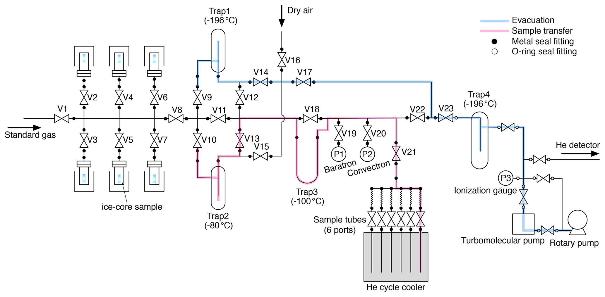
A schematic diagram of our extraction system is shown in Fig. 1. The components of the extraction line (tubings, fittings, valves and vessels) are made of electropolished (EP) stainless steel except for traps made of Pyrex glass. Traps 1–3 have Kovar glass-to-metal transition. It has six inlet ports for stainless-steel vessels, each containing an ice-core sample. The vessels and traps 1–3 are connected to the line with metal face-seal fittings (Fujikin UJR®, 1/2 in., 12.70 mm) using nickel gaskets. Diaphragm metal-seal valves (Fujikin FUDDFM-71G-9.52) are used for all stop valves (V1–V23). All valves are manually operated. ISO-KF25 flanges are attached to both ends of Trap 4 with two-component epoxy adhesive, and Viton o-rings are used for connecting the trap to the line. The vacuum is provided by a turbomolecular pump (Pfeiffer HiPace 80) backed by an oil rotary pump (Edwards). The vessels are made of stainless-steel pipe (65A) with ConFlat flange (ICF114) with a volume of ∼ 600 mL, and the sample tubes are made of 1/4 in. (6.35 mm) EP stainless-steel tube with a metal-seal valve (Fujikin FUDDFM-71G-6.35) with a volume of 6.6 mL.
After constructing the extraction line (before actual use), we performed pre-treatment of inner surfaces of all the lines, vessels and sample tubes as follows. Pure O2 (> 99.999 %) was humidified by bubbling through pure water in a glass flask sealed with a silicone cap at room temperature and flowed into the lines and vessels heated to 90–100 ∘C with heating tapes at a flow rate of ∼ 20–50 mL min−1 for 2 weeks to remove trace organic substances and hydrocarbons efficiently. After the treatment, the line and vessels were evacuated at 90–100 ∘C by a turbomolecular pump for 1 week. The same treatment is applied to the sample tubes for air extraction. We note that we use a different set of sample tubes with a better performing treatment after splitting for δO2∕N2 stability (GOLD EP WHITE, GEPW, tubes; see below), but the H2O + O2 pre-treatment is sufficient for the extraction step and has the advantage of low cost.
2.1.2 Preparation of apparatus and ice samples
For routine air extraction, the sample tubes and extraction line are evacuated overnight to < 1.3 × 10⁻⁴ Pa (measured at the head of the turbomolecular pump with an ionization gauge, P3). If no extraction is planned for 2 d or more, the sample tubes and extraction line are filled with pure air (> 99.99995 %) at ∼ 500 Pa. On the day of air extraction from ice-core samples, Trap 4 is cooled to −196 ∘C by liquid nitrogen to evacuate further the sample tubes and extraction line (< 10−4 Pa). The vessels are brought out from an oven at 50 ∘C and cooled to room temperature in ∼ 30 min and then brought to the cold room at −20 ∘C for further cooling. Ice-core samples of ∼ 90–150 g, typically 7 to 12 cm long, are cut out from bulk ice-core samples with a band saw in a cold room at −20 ∘C. The same band saw is used to trim all faces for rough decontamination, removing ∼ 2–11 mm from the original surfaces. The inner ∼ 50–70 g of ice is used for the air extraction, and the removed outer ice is stored for other measurements (e.g., for multiple analyses in case of measurement failures). The amount of ice may be reduced to ∼ 35 g for all measurements with somewhat lower precision and to ∼ 9 g if only MS measurements are conducted (without sample splitting).
After cutting out an ice sample from the stored ice-core body, the exposed outer parts of the stored ice-core sections are trimmed with a band saw, and all the sections are shaved off by a ceramic knife. The shaving by knife also enables the visual inspection of the ice for any cracks. We found that more than 8 mm should be removed for the Dome Fuji clathrate hydrate ice (>∼ 1400 m) to eliminate gas-loss fractionation of δO2∕N2 and δAr∕N2 due to diffusive gas loss during ice storage (details are described in Sect. 5.2). The cleaned ice sample is placed in a pre-cooled extraction vessel and sealed with a ConFlat flange and copper gasket. The vessels are placed in a dewar that accommodates a copper tube (o.d. = 78 mm, i.d. = 74 mm, height = 135 mm) and a eutectic refrigerant bag (∼ 1000 g, pre-cooled to −50 ∘C) to keep the ice temperature below −25 ∘C.
2.1.3 Manipulations for air extraction
Up to six vessels, thus prepared, are brought to our laboratory at room temperature. All valves on the extraction line are closed, and the closed-cycle refrigerator is turned on. Then, pure air is introduced from V16 to purge the manifold for vessels, and the vessels are connected to the line. The room air is evacuated from the vessels with the turbomolecular pump. After ∼ 5 min when the pressure after two water traps (i.e., without water vapor) is below 10−2 Pa, the flanges and connections are leak tested with a helium leak detector (< 10−8 Pa L s−1). Then, pure air is introduced into the vessels and pumped out four times to further remove room air from the vessels. All the vessels are then evacuated for 90 min through the evacuation line (Fig. 1, blue). Typically, four to six samples are simultaneously evacuated. The evacuation is made to remove residual room air from the vessels as well as to sublimate the ice surface for further cleaning of the sample. Then, the vacuum line is switched to the sample transfer line (Fig. 1, pink), which is the line for transferring sample air during the extraction, by closing V8, V9, V14 and V17; cooling traps 2 and 3 to −80 ∘C with ethanol; and opening V22, V13, V10 and V8. The evacuation continues for another 30 min.
After the evacuation, all but one of the vessels are isolated by closing the valves above them (V2–V7). V19 and V21 are opened, and the open vessel and line are evacuated for another ∼ 5 min. V22 is closed to stop the evacuation, and the valve of a sample tube is opened to establish the line for sample air transfer. The ice sample is then melted by immersing the vessel in a hot water bath (∼ 90 ∘C) by a few millimeters from the bottom. The air released from the melting ice is continuously transferred into the sample tube at ∼ 10 K, after passing through two water traps at −80 and −100 ∘C. The first trap has sufficient inner volume to condense a large amount of water vapor, and the second trap contains fine glass tubes for high trapping efficiency. Sample transfer is monitored by a Baratron gauge (MKS, full scale = 1333 Pa) (P1 in Fig. 1), which measures the sample air pressure in the line without water vapor. The maximum pressure during the transfer is ∼ 100–200 Pa. The hot water bath is removed after the completion of ice melting (judged by the change of noise and temperature at the bottom of the vessel sensed by the operator). When the pressure decreases below the detection limit (0.1 Pa), the sample transfer is considered to be complete, and the valve of the tube is closed. Residual pressure in the transfer line is measured using a Convectron gauge (Granville-Phillips, P2 in Fig. 1) (typically < 2 × 10⁻² Pa). The melting of the ice sample takes < ∼ 3 min, and the remaining air transfer takes ∼ 7 min after the melting. Finally, the valve of the vessel is closed, and the line is evacuated for ∼ 2 min to decrease the pressure to < 10−4 Pa (P3).
The pressure in the next vessel is measured with the Baratron gauge (P1) by closing V20, V21, and V22 and opening the valve of the vessel (typically < 1 Pa for the second vessel and ∼ 4 Pa for the fifth vessel, because of gradual accumulation of air released from ice samples). This ensures the absence of a leak through the valve above the vessel and hence the quality of the sample air in the previous extractions. Then, V22 and V21 are opened, and the line and vessel are evacuated for ∼ 5 min, the ice sample is melted, and the released air is transferred to the next sample tube. We repeat these procedures until all the extractions are completed.
After collecting the air from all prepared samples, the sample tubes are removed from the helium cycle cooler and laid in the laboratory room with ambient temperatures for 15–24 h. All the vessels and traps are also disconnected from the line, rinsed with pure water and placed in ovens at 50 ∘C for drying. The mass of Trap 1 is measured before and after extraction to estimate the total mass of sublimated ice during the evacuations (typically 0.5–1.5 g from four to six samples). Finally, as the preparation for the next extractions (on the following day or after), another set of sample tubes and traps are connected to the line and evacuated with the turbomolecular pump (to < 10−2 Pa), and then the line is checked with a helium leak detector (< 10−8 Pa L s−1). After the leak check, the tubes and the line are evacuated until the next extractions.
2.2 Splitting
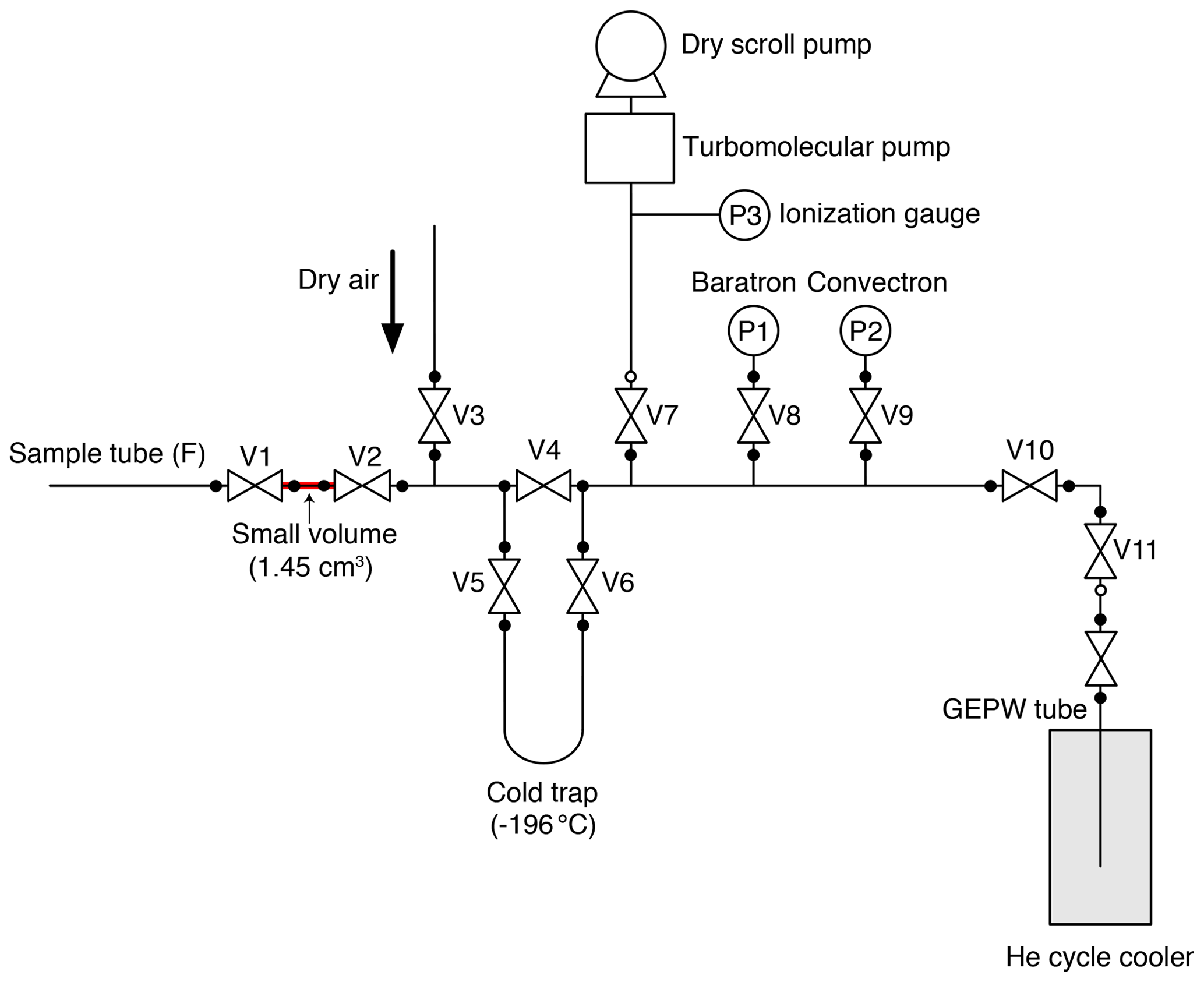
A small aliquot of air is separated from the sample tube and transferred to a second tube using the split line (Fig. 2) for MS analysis. We employed the general design of the line for noble-gas measurements developed at SIO (Orsi, 2013; Bereiter et al., 2018). The split line is made of electropolished stainless steel except for a U-shaped cold trap made of Pyrex glass and connected to the line with bored-through 3/8 in. (9.53 mm) ultra-torr fittings (Swagelok). A diaphragm metal-seal valve (Fujikin FUDDFM-71G-6.35) is placed next to the sample tube (V1) for splitting, and stainless-steel bellow valves (Swagelok SS-8BW or SS-4H) are used for other valves. The vacuum is provided by a turbomolecular pump (Pfeiffer HiPace80) backed by a dry scroll pump. The same pre-treatment with humidified O2, as applied to the extraction line, is employed for the split line. To minimize the consumption of O2 at the metal surfaces leading to depletion of the δO2∕N2 ratio during the sample storage in the tube, a passivation treatment (GOLD EP WHITE, Nissho Astec Co. Ltd.) is employed, which forms a passive layer of oxidized chromium on the stainless-steel surface (hereafter, this type of tube is called GEPW). In our experiences, stainless-steel sample tubes with mechanical polishing or electropolishing may lead to an unacceptable depletion of δO2∕N2 (e.g., by −5 ‰) in less than 8 h because of the O2 consumption. The GEPW tubes do not deplete δO2∕N2, and thus the storage correction is not necessary (see Sect. 4.2.1).
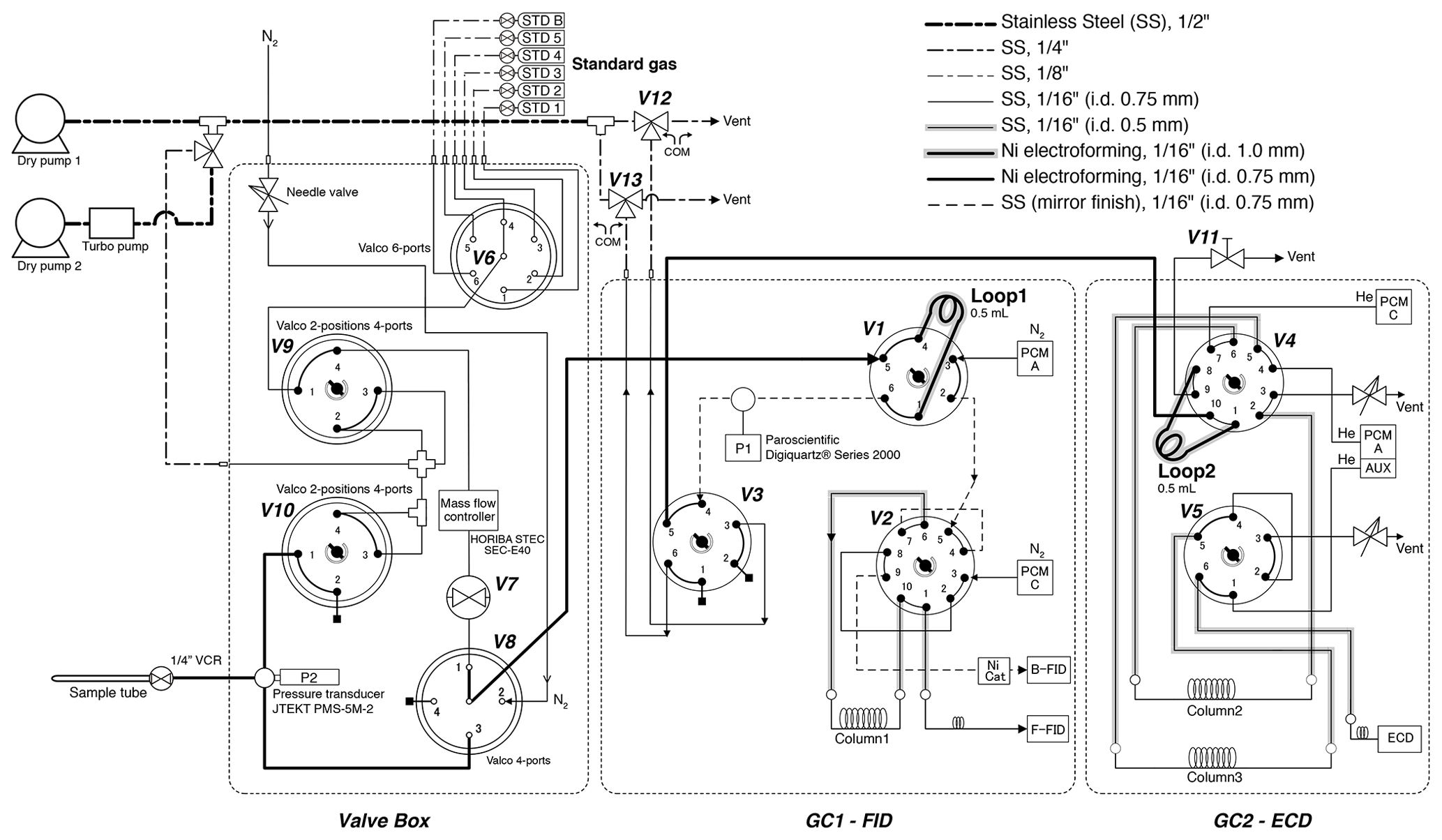
Figure 3Schematic diagram of gas chromatographs and inlet. All two-position valves are in “off” positions.
The experimental procedures are as follows. The split line is filled with pure air (> 99.99995 %) at ∼ 500 Pa when not in use, and it is evacuated for more than 30 min before the splitting. The GEPW tubes are evacuated overnight. The sample tube containing ice-core air is connected to the split line with a 1/4 in. (6.35 mm) UJR® fitting using a silver-plated nickel gasket. The GEPW tube is inserted in a helium cycle cooler at < 10 K and connected to an adapter with a VCR® fitting, which is then connected to the split line with a VCO® fitting (Swagelok). The whole line is evacuated for ∼ 30 min, during which the pressure decreases to < 3 × 10⁻⁵ Pa (P3). After a leak check, V1 is closed, and the valve on the sample tube is opened to expand the sample air into the small volume (1.45 mL) between the valves. The time required for equilibration of the air composition in the small volume with the sample tube is > 20 min. During this waiting time, the sample air may be fractionated if the temperature gradient exists between the tube and the small volume. To minimize such fractionation, the sample tube and small volume are covered with a sheet of bubble wrap so that air conditioners on the laboratory ceiling do not directly blow against the splitting part. The expanded air is then split by closing the valve of the sample tube. The air in the split volume is transferred to the GEPW tube for 5 min, after passing through the cold trap at −196 ∘C to remove CO2 and N2O. The sample transfer is monitored by measuring the pressure of the line with a Baratron gauge (MKS, full scale = 1333 Pa) (P1 in Fig. 2). The GEPW tube is lowered by a few centimeters into the helium cycle cooler when the pressure drops below 1.0 Pa to improve the trapping efficiency of the gas by exposing fresh metal surface. The air transfer is complete in 5 min, and the valve of the GEPW tube is closed. The residual pressure is measured using a Convectron gauge (Granville-Phillips) (P2 in Fig. 2), and the GEPW tube is disconnected from the line. The GEPW tube is warmed to room temperature and allowed to homogenize the sample air for at least 3 h before the MS analysis (the longest waiting time is ∼ 20 h). The air remained in the original sample tube is used for measuring CH4, CO2 and N2O concentrations as well as total air content.
3.1 CH4, N2O and CO2 concentrations
3.1.1 Gas chromatography
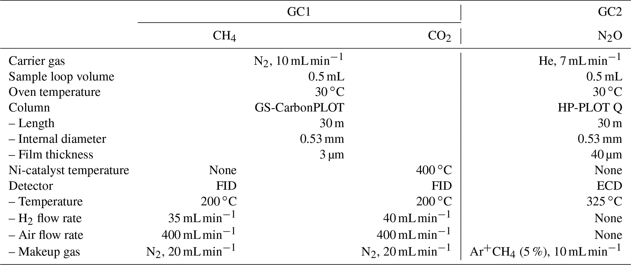
After taking the aliquot of air for the mass spectrometer analysis, the remaining air in the original sample tube (∼ 80 % of the extracted air) was measured for the concentrations of CH4, CO2 and N2O with two gas chromatographs (Agilent 7890A) (Fig. 3). The settings of the GCs are summarized in Table 1. Briefly, CH4 and CO2 are measured with one GC (GC1) equipped with two flame-ionized detectors (FIDs) (CO2 is converted to CH4 by nickel catalyst), and N2O is measured with another GC (GC2) equipped with an electron capture detector (ECD). We employ capillary columns to obtain high separation and narrow peaks. CH4 and CO2 are separated with a GS-CarbonPLOT (Agilent) capillary column (L = 30 m, i.d. = 0.53 mm, film thickness = 3 µm), and N2O is separated with a HP-PLOT Q (Agilent) column (L = 30 m, i.d. = 0.53 mm, film thickness = 40 µm). We use N2 (> 99.99995 %, Taiyo Nissan Corp., Japan) for carrier and makeup gases, and we use H2 (> 99.99995 %, Taiyo Nissan Corp., Japan) for FID for GC1. Hydrocarbon-free air for FID is generated by a zero-air generator (PEAK Scientific, ZA015A). For GC2, we use He carrier (> 99.99995 %, Taiyo Nissan Corp., Japan) for high separation, and we use the mixture of Ar and CH4 (5 %) as makeup gas for high sensitivity. We use two gas purifiers in series (a Mini Fine Purer from Osaka Gas Liquid and a Big Universal Trap from Agilent) for the carrier, makeup and H2 gases to ensure their purity. Zero air is further purified with a Hydrocarbon/Moisture Trap (Agilent).
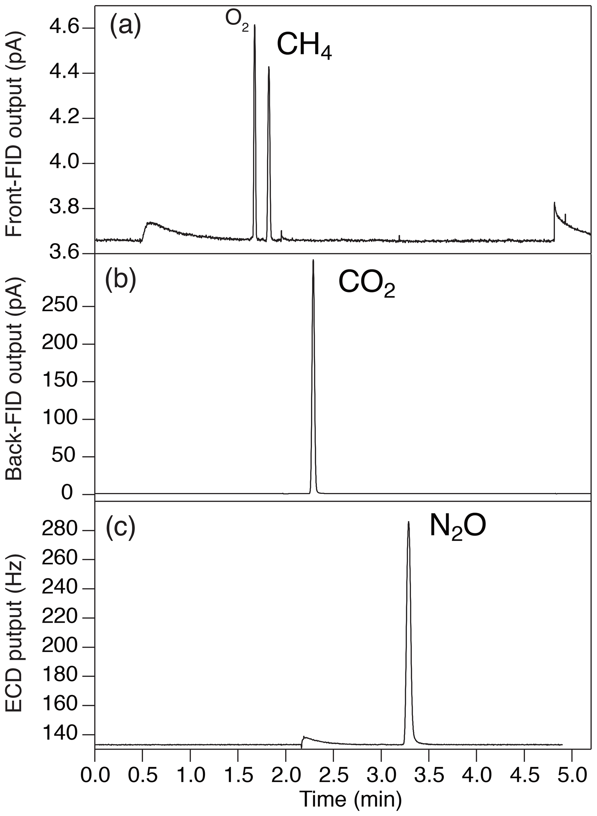
Figure 4Typical chromatogram of (a) front FID for CH4 (the largest peak is O2, and the second-largest peak is CH4), (b) back FID for CO2 and (c) ECD for N2O.
To measure a small amount of sample gas, we use 0.5 L sample loops (Loop 1 and 2 in Fig. 3) filled at sub-ambient pressure. Small sample loops are also effective in reducing baseline fluctuations when GC valves are switched. The dead volumes of the inlet, fittings and tubing need to be minimized for filling the loops at sufficient pressure. We achieve the total volume (sample loops and dead volumes) of 3.3 mL by using 1/16 in. (1.59 mm) tubing (0.7 or 1.0 mm i.d.), a customized metal-seal fitting (VCR) with a small bore (1.5 mm i.d.) for the connection of the sample tube and a customized bracket with small dead volume for the pressure transducer at the inlet (machined Valco cross fitting). This configuration allows us to fill the sample loops at 400–600 hPa for the first injection and 300–500 hPa for the second injection, for typical ice-core measurements. The third injection is necessary if the pressure for the first injection exceeds the range of calibration or if a gas handling error occurs. To minimize the broadening of the CO2 peak by passing through the nickel catalyst (Agilent G3440-63002), we replaced the 1/4 in. (6.35 mm) o.d. tube for packing the catalyst with a 1/8 in. (3.18 mm) tube. To minimize adsorption/desorption of trace gases on the inner walls of the tubing, we employ VICI electroformed Ni tubing or mirror-polished stainless-steel tubing (Labosoltech). Typical chromatograms are shown in Fig. 4.
A standard gas measurement at atmospheric pressure is conducted as follows. V8 is set to position 1, V1 is set to off, V3 is set to off and V7 is opened to allow the standard gas to flow through the two sample loops at 100 mL min−1 for 1.0 min using a mass flow controller (HORIBA STEC, SEC-E40). V7 is closed to stop the gas flow, V3 is set to on to disconnect the two GCs, and the GC measurements are initiated by switching V1 and V4 to let the carrier gases to flow through the sample loops. In GC1, CH4 separated by column 1 is detected with the front FID (retention time ∼ 1.8 min). At 1.74 min, V2 is switched to let CO2 from column 1 pass through the Ni catalyst (to convert to CH4) and then to the back FID (retention time ∼ 2.3 min). Finally, at 4.6 min, V1 and V2 are switched to the original positions. In GC2, immediately after N2O passes through column 2 (at 1.5 min), V4 is switched to back-flush column 2 to vent H2O out from the GC during the run. It is important to prevent the accumulation of H2O in the columns, which may cause an unstable baseline during later measurements. N2O is further separated in column 3, and V5 is switched at 1.95 min to lead N2O to ECD (air eluting before N2O is vented to the atmosphere). Finally, at 4.89 min, V5 is switched to the original position. After the run, the sample loops are evacuated to < 0.25 hPa (P1) (Paroscientific Digiquartz® Series 2000, absolute 0.16 MPa full scale).
For a standard gas measurement at sub-ambient pressure, the sample loops are first evacuated for ∼ 30 min by closing V11, switching V12 and V13 (to connect the sample loops and dry pump 1), and turning V3 on. Then, the standard gas is allowed to flow through Loop 1 by turning V8 to position 1, and V7 is opened. The flow rate is 100 mL min−1 for 1 min and then 17 mL min−1 for 1 min. V3 is turned off to isolate the pump and start filling the sample loops. When the pressure (P1) reaches a prescribed value, the flow is stopped by closing V7. Then, 15 s is allowed to stabilize the pressure and the temperature of the sample loops, and the GC measurements are initiated by switching V1 and V4 simultaneously to introduce the carrier gases to the sample loops. The measurement procedures of the GCs are the same as above.

The routine GC calibration and measurement procedures are as follows. We use three standard gases to cover the ranges of greenhouse gas concentrations in the samples (details of our working standard gases are described in the next section and summarized in Table 2). On each day of the measurement, the standard gases in the lines (1/8 in. (3.18 mm) tubes) connecting the cylinders and GC inlet are first pumped out for 5 min with a dry pump, and the standard gases are freshly introduced from the cylinders into the lines. The rest of the standard gas handling and measurements are automated with a custom-made software (with LabVIEW). First, the overall stability of the GC system is assessed by measuring the three standard gases three times at atmospheric pressure. For each standard gas, the peak areas of three consecutive measurements must agree within 1 % to proceed. The linearities of the detector responses are also checked by comparing the middle standard gas concentrations calculated from linear interpolation of the concentration–area relationships of high and low standard gases with the original values. The typical differences are +1.1 ± 1.7 ppb for CH4, −0.3 ± 0.2 ppm for CO2 and +2.3 ± 1.2 ppb for N2O. Then, each of the three standard gases is measured at three sub-ambient pressures (i.e., nine measurements in total) to construct calibration curves for the ice-core measurements. Typical pressures are 300, 400 and 500 hPa to cover the pressure range for two injections of sample air from ∼ 60 g of ice.
After all the standard gas measurements, a sample tube is connected to the GC inlet by VCR, V8 is set to position 4, V10 is switched on to evacuate the inlet with a turbomolecular pump for ∼ 20 s and the VCR connection is leak-checked with P2 (JTEKT PMS-5M-2 pressure transducer). The inlet and two sample loops are then evacuated via V10 and V3, respectively, for 15 min to < 0.25 hPa, V10 is closed, the sample gas is expanded into the inlet by opening the stop valve on the sample tube and the controlling software is started. Three seconds later, the two sample loops are connected and isolated from the vacuum line (V3 off), and the sample air is expanded into the sample loops (V8 position 3). The rest of the GC measurement sequences are the same as the standard gas measurements. After measuring a sample, the sample loops are evacuated by switching V3 for 3 min (P1 < 0.25 hPa), and the second measurement is initiated automatically. After the end of the second measurement, the sample tube is replaced with the next one.
After measuring all samples, the standard gases are measured again at the sub-ambient pressures to account for the drifts of GC signals during the sample measurements. The areas of the standard gases before and after the sample measurements were linearly interpolated to the time of the sample measurements for calculating the sample concentrations, assuming that the drift is linear with time.
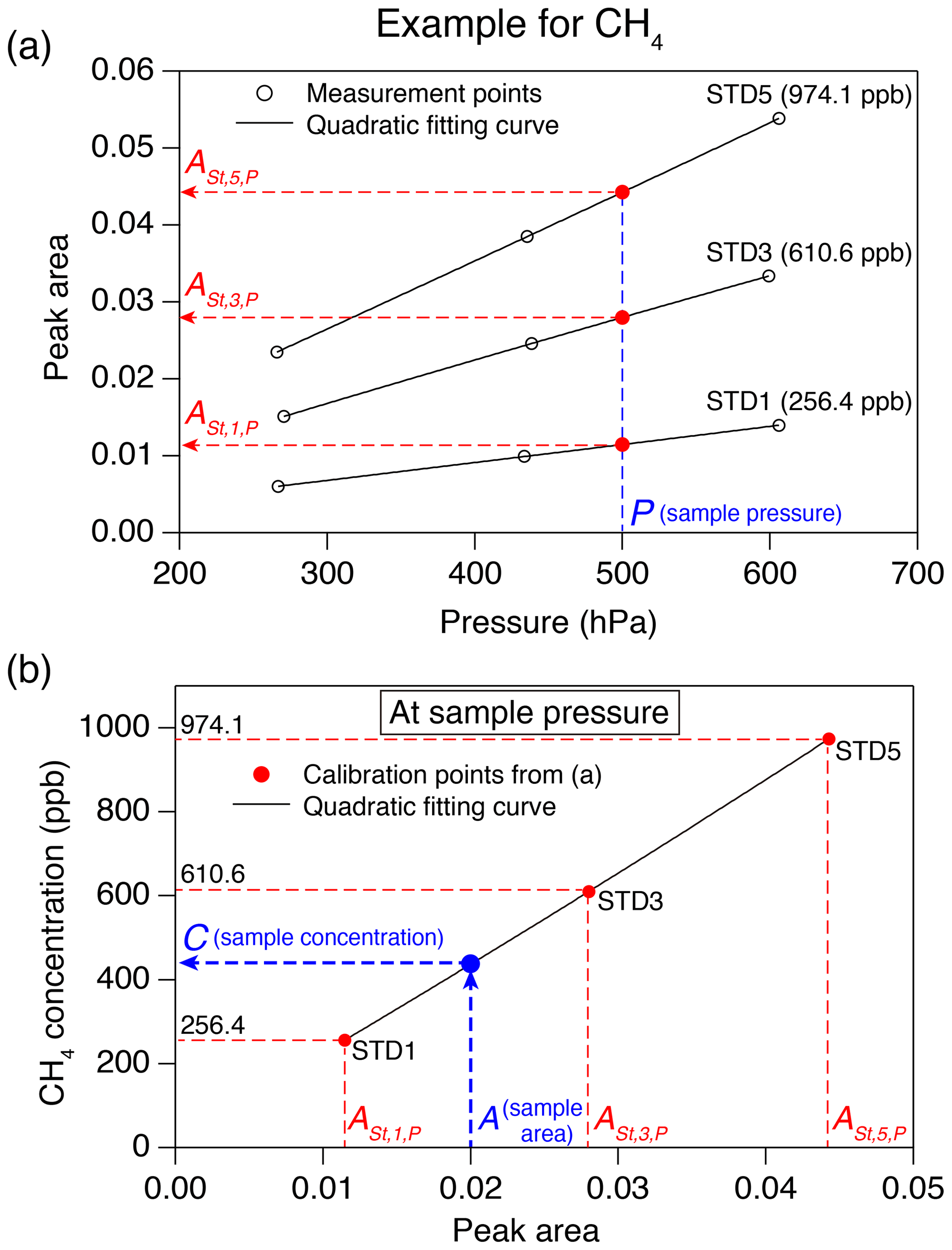
Figure 5Example of a calibration procedure for greenhouse gas concentration. (a) Peak areas for three standard gases measured at three pressures (black circles), with quadratic fits (black lines). Peak areas of the standard gases (, , and , red circles) estimated at the sample pressure (blue dashed line) are also shown. (b) Calibration curve at the sample pressure (black line) from the peak areas from panel (a). The numbers in the panel are CH4 concentrations of the standard gases, A is the peak area of the sample and C is the CH4 concentration of the sample.
The concentration of greenhouse gas in the sample air is determined based on the calibration measurements of the three standard gases at three pressures. As an example, the calibration procedure for CH4 concentration is schematically shown in Fig. 5. First, the peak areas of the three standard gases at the sample pressure (in the sample loop) are estimated by
where is peak area of standard gas n (=1, 3 and 5) calculated for the sample pressure (P), and an, bn and cn are coefficients obtained by second-order polynomial fit to the peak area vs. pressure from the calibration measurements (Fig. 5a). The greenhouse gas concentration in the sample is obtained by
where C is concentration; A is sample peak area; and d, e and f are coefficients obtained by the second-order polynomial fit to the standard gas concentrations vs. (n=1, 3 and 5) (Fig. 5b). Each sample air is measured at least twice, and the mean values are used.
3.1.2 Standard gases
The CH4, N2O and CO2 concentrations are determined against Tohoku University (TU) scales, which are based on gravimetrically prepared primary standard gases (Aoki et al., 1992; Tanaka et al., 1983). Uncertainties of the TU primary standards are < ± 0.2, 0.2 and 0.03 % for CH4, N2O and CO2 concentrations, respectively (Aoki et al., 1992, for CH4; Ishijima et al., 2001, for N2O; and Tanaka et al., 1987, for CO2). The ice-core standard gases are calibrated using the primary standard gases manufactured in 2008 for CH4 (300.1–2799.1 ppb) and CO2 (200.13–449.72 ppm) and those made in 1991 for N2O (100.0–400.1 ppb). Working standard gases at NIPR contain CH4, N2O and CO2 in purified air in 47 L aluminum cylinders (Taiyo Nissan Corp., Japan), whose concentrations were calibrated at Tohoku University using their working standard gases named “2007-Ice-Work” (with 25 measurements for each cylinder). We have five working standard gases (named STD 1–5) with different concentrations covering from preindustrial Holocene to glacial maxima (Table 2). Two additional cylinders (STD-A and B) are prepared and calibrated against the NIPR working standard gases at NIPR and used for various tests. Uncertainties of CH4, N2O and CO2 concentrations of the NIPR working standards are < ± 0.6 ppb, ± 0.3 ppb and ± 0.02 ppm, respectively (1 standard error of the mean).
For modern atmospheric concentration levels, the TU scales are in agreement with the NOAA/WMO scales within ∼ 2 ppb for CH4, ∼ 0.3 ppm for CO2 and ∼ 0.5 ppb for N2O as reported in the WMO/IAEA Round Robin Comparison Experiment (Dlugokencky, 2005; Tsuboi et al., 2017) (https://www.esrl.noaa.gov/gmd/ccgg/wmorr/index.html, last access: 10 December 2020.). However, at lower concentration levels, inter-calibration between TU and NOAA scales has not been conducted. For CH4 and N2O, we discuss the consistency of calibration scales by comparing our ice-core data with those from other laboratories (see Sect. 5.1).
3.2 Mass spectrometry for isotopic and elemental ratios of N2, O2 and Ar
Isotopic and elemental ratios (δ15N∕14N of N2, δ18O∕16O of O2, δO2∕N2 and δAr∕N2) are analyzed on a dual-inlet mass spectrometer (Thermo Fisher Scientific, Delta V) with nine Faraday cups and amplifiers to simultaneously collect ion beams of molecular masses 28, 29, 32, 33, 34, 36, 38, 40 and 44. The registers, typical beam intensities and other MS settings are given in Table 3. While we collect raw data from all of these cups, we do not use the signals of masses 33, 36 and 38 in this paper because high-precision values for isotopic ratios with these masses (including appropriate corrections for interference and nonlinearity in the mass spectrometer) are not established. To achieve high precision, we control the temperature around the mass spectrometer (especially around the inlet) by isolating the mass spectrometer from the room-air temperature fluctuation with plastic sheets and introducing temperature-controlled air generated by an air conditioner (Orion PAP03B) into the booth. Two large (∼ 45 cm diameter) and a small (∼ 20 cm diameter) fans in the booth vigorously mix the air to maintain the temperature around the inlet at 25.7 ± 0.3 ∘C all year round.

3.2.1 Measurement procedures
Our reference gas is commercially available purified air (> 99.9999 %, Taiyo Nissan Co.) in a 47 L cylinder filled in 3 L electropolished stainless-steel containers (hereafter reference cans), each with two bellow-seal valves (Swagelok SS-4H) creating a small pipette volume (1.3 mL) at the exit. The inner surface of the can is preconditioned by humidified O2 at > 120 ∘C as for the extraction line. The reference can attached to the standard side is rarely disconnected.
Our mass spectrometry largely follows Severinghaus et al. (2009). Prior to the daily sample measurements, a reference can is connected to the sample port of Delta V using a VCO® fitting (typically on the prior evening to stabilize the can's temperature), and the ports and pipettes are evacuated. The MS valves leading to the reference cans are closed, and both bellows are evacuated for 5 min. Then, the MS valves to the inlet ports are opened to check for leaks using an ion gauge, and all bellows and lines are further evacuated for 5 min. On both sides, the reference gas is introduced into the pipette of the can by closing the valve at the MS side and opening the other valve, and they are equilibrated for 10 min. The pipette volumes are disconnected from the cans, and the aliquots are expanded into the bellows and equilibrated for 10 min. Then, the bellows are isolated from the inlet and compressed to reach ∼ 34 mbar. The initial pressure in the fully expanded bellows is ∼ 28 mbar from a freshly filled can. The reference can is replaced by a new one when the initial pressure decreases to ∼ 18 mbar.
The reference gas from the sample port is measured against the standard side (can vs. can) for four blocks to check the SDs. Before each block, the acceleration voltage is optimized by centering the mass 40 peak, the background is measured after a 120 s idle time and the pressures are adjusted to 5000 ± 50 mV for mass 28 (3 × 10⁸ Ω), automatically with the ISODAT software. The idle time and integration time are 10 and 16 s, respectively. Each block consists of 17 changeover cycles, and only the latter 16 values are used. After running the four blocks, two blocks are run by unbalancing the sample pressure by ± 10 % against the standard side for obtaining pressure imbalance sensitivity (see below).
The GEPW tube containing the sample air is connected to the sample port, and the sample port is evacuated during the previous measurement. The procedure of the sample measurement is the same as the can vs. can measurement, except that the sample expansion into the bellow is made in one step by simply opening the tube valve. We run two blocks for each sample to obtain a total of 32 cycles. Typical SDs in 1 block (16 cycles) are 0.013 ‰, 0.029 ‰, 0.010 ‰ and 0.017 ‰ for δ15N, δ18O, δO2∕N2 and δAr∕N2, respectively.
3.2.2 Pressure imbalance and chemical slope corrections
The ratios of ion currents of different masses are slightly sensitive to the pressure in the ion source; thus a correction is applied with an established procedure (Severinghaus et al., 2003). The pressure imbalance sensitivity (PIS) is a slope of δ values against differences in beam intensity (, where I is the mean beam intensity in one block), which is determined by measuring the reference gas at the sample side at three pressures (at ΔP=0, +10 % and −10 %). The PIS is measured every day and used for correcting the sample values measured on the same day by
The PIS gradually changes over several weeks, and it shifts after a filament replacement.
Relative ionization efficiencies of gas are also sensitive to variations in the mixing ratio of the gas in total air (the sensitivity is called “chemical slope”) (Severinghaus et al., 2003). The chemical slopes are determined from the measurements of the reference gas added by pure O2 (+10 %, +20 % and +30 % of original O2 amount) for δ15N and pure N2 (+10 %, +20 % and +30 % of original N2 amount) for δ18O. The correction is made by
where CS1 and CS2 are chemical slopes for δ15N and δ18O, respectively. The chemical slopes are fairly stable and thus are measured only a few times per year. The typical values of CS1 and CS2 are 0.0005 ‰∕‰ and 0.0018 ‰∕‰, respectively.
The final normalization against the modern atmosphere (the ultimate standard gas for ice cores by definition) requires thorough investigation of the stability of reference gases and the atmospheric ratios, which we discuss in Sect. 4.2.
3.3 Total air content
Table 4Test results using a standard gas (STD-A) for greenhouse gases.

Values are differences from the calibrated concentrations of the STD-A cylinder (Table 3).
Total air content (TAC) is the amount of occluded air in a unit mass of ice (mLSTP kg−1) (Martinerie et al., 1992). In our system, TAC is calculated from
where P is pressure in the sample loops upon first expansion; T is air temperature near GC; m is mass of ice sample just before melting; and Va, Vb and Vc are the volume of the sample tube, the volume of the pipette at the split line, and the combined volume of GC inlet and sample loops, respectively. To take into account the ice mass loss during the evacuation, m is estimated from
where minitial is the initial ice mass measured in the cold room, mTrap1 is the ice mass in Trap 1 after all extractions for a day measured in the laboratory, rt () is the ratio of total evacuation time to the time of the first evacuation through Trap 1 (120/90 min), and nsample is the number of samples for the day. The ice loss for each sample thus estimated is 0.1–0.3 g.
Va and Vb were determined manometrically against a known volume (118.7 mL) with a pressure gauge (Paroscientific Digiquartz® model 745-100A, absolute 0.69 MPa full scale). The whole apparatus is first evacuated, and the air is introduced from a cylinder into the glass flask at about atmospheric pressure. The air is expanded into the manifold, pipette, and tube, and the pressure measured at each step is used to calculate the volumes by the ideal gas law. The expansion and recording are repeated 10 times, and they are averaged.
Similarly, Vc was determined manometrically for each sample tube (∼ 6.6 mL), which was attached to the GC inlet. N2 or air in a sample tube at a known pressure was expanded into the evacuated GC inlet and sample loops, and the pressure was recorded (valve on the sample tube is kept open). The expansions/evacuations were repeated a few times, and the gas in the sample tube was re-filled. The whole procedures were repeated a few times to obtain a total of 12 measurements for each tube.
The calibration of the volumes Va, Vb and Vc must be made for individual sample tubes because the volumes in the valves and end connections are slightly different from each other (Va, Vb and Vc are different by up to 0.8 %, 0.6 % and 0.5 %, respectively, between the tubes). Average Va, Vb and Vc are 6.6, 1.4 and 3.4 mL, respectively. The standard error of the mean for the 10–12 measurements of Va, Vb and Vc are 0.04 %, 0.10 % and 0.04 %, respectively. By propagating these values and the uncertainties of temperature (assumed to be 1 K), pressure (assumed to be 16 Pa) and ice mass (assumed to be 0.1 g), 1σ uncertainty of TAC is estimated to be 0.5 mLSTP kg−1.

Figure 6Standard gas (STD-A) composition measured against reference gas for (a) δ15N, (b) δ18O, (c) δO2∕N2 and (d) δAr∕N2. Filled markers represent samples transferred only through the split line, and open markers represent samples transferred through both extraction and split lines. Vertical grey lines indicate the timing of replacements of the reference can, and vertical light blue lines indicate the timing of filament replacements.
During air extraction, splitting and analyses, alteration of air composition may occur for various reasons, such as gas dissolution or chemical reaction in the meltwater, degassing from inner surfaces of vessel and line, and diffusive fractionations of isotopic ratios. Below, we evaluate the performance of the tubes, apparatus and instruments by various tests and controlled measurements (mimicking ice-core analyses with standard gas and gas-free ice).
4.1 CH4, N2O and CO2 concentrations
4.1.1 Tube storing test
We evaluate the concentration changes during gas storage in the sample tubes and test tubes (used for injecting standard gas to the apparatus, with metal-seal valves at both ends) by filling standard gas from a cylinder (STD-A) into evacuated tubes and measuring the sample tubes on the following day and the test tubes on the same day. The changes in CH4, N2O and CO2 concentrations thus obtained are insignificant with respect to the measurement precision for both the sample tubes (+0.8 ± 2.1 ppb, +1.3 ± 2.1 ppb and +0.1 ± 1.1 ppm, respectively, with n = 25) and test tubes (+0.7 ± 2.2 ppb, +0.9 ± 1.0 ppb and −0.2 ± 0.1 ppm, respectively, with n = 17) (Table 4). The excellent results of the storing tests are attributable to the passivation treatment of the tubes and the use of valves with clean inner surfaces (Fujikin metal diaphragm valves). We note from our earlier experience that CH4 is produced by up to several parts per billion by opening and closing metal bellow valves (Swagelok SS-4H) if they become old (after several hundred operations) and that CO2 concentration increases by up to ∼ 10 ppm if the passivation treatment is insufficient.
4.1.2 Standard gas transfer test
Gas-free ice for tests are made from ultra-pure water in a stainless-steel vessel (∼ 1800 mL) sealed with a ConFlat blank flange. The water is boiled for 20–30 min with an open outlet port on the flange, cooled to room temperature after closing the outlet and then put in a freezer at −20 ∘C. The side of the vessel is surrounded by insulation so that the water is frozen from the bottom over a few days. The ice is removed from the vessel, and ice with visible cracks and bubbles is removed (more than half of the ice).
Standard gas from a cylinder is flushed through a pre-evacuated line and test tube (volume is 3 or 5 mL) at 50 mL min−1 for 5 min and sampled at atmospheric pressure after ceasing the flow by closing an upstream valve. The relatively low flow rate for flushing prevents thermal fractionation of the gas due to adiabatic expansion at the pressure regulator (important for isotopic analyses), and the pre-evacuation and > 200 mL of total flow ensure clean sampling.
The test tube with standard gas and vessel with ∼ 50 g of gas-free ice are attached to the extraction line, and the vessel is evacuated for 120 min. The ice is melted while the vessel is evacuated (for 15 min) to remove any air degassed from the melt. We also use ice-core melt instead of gas-free ice melt for the blank test. In this case, the vessel with ice-core melt is evacuated for 30 min after a sample extraction to pump out any residual air. Then, the standard gas from the test tube is slowly injected into the extraction system and transferred continuously over the gas-free water into a sample tube, maintaining the pressure similar to that of ice-core extraction.
The standard gas thus transferred to the sample tubes is measured on the following day, after handling it with the split line (see below for the results of isotopic analyses). No significant changes in CH4, N2O and CO2 concentrations are observed with respect to the mean values of the test tubes' storing tests (+0.8 ± 2.7 ppb, −0.1 ± 1.7 ppb and +1.3 ± 0.7 ppm, Table 4). Based on the above results, we apply no corrections for CH4, N2O and CO2 concentrations.
4.2 Isotopic and elemental ratios of N2, O2 and Ar
4.2.1 Storing test of GEPW tubes
To evaluate the possible effect of gas storage in the GEPW tubes for 1 d, the reference gas was transferred to the tubes using the split line and measured the following day, and the results were compared with those measured on the same day. They are identical within the measurement uncertainties for all ratios (−0.002 ‰ ± 0.003 ‰ for δ15N, −0.002 ‰ ± 0.010 ‰ for δ18O, −0.012 ‰ ± 0.056 ‰ for δO2∕N2 and −0.013 ‰ ± 0.042 ‰ for δAr∕N2, with n=14); thus no corrections are applied for the storage duration in the GEPW tubes.
4.2.2 Standard gas transfer test
The standard gas filled in a test tube was transferred to a sample tube with the extraction line and gas-free water (the same experiment as in Sect. 4.1.2), and an aliquot was taken with the split line and transferred to a GEPW tube as the ice-core analysis (Fig. 6). On the other hand, the same standard gas filled in the same test tube was attached directly to the split line, and its aliquot was transferred to a GEPW tube, skipping the extraction line and overnight storage (Fig. 6). Comparison of the measured values from these two experiments gives the changes in the isotopic and elemental ratios during the ice-core air extraction and overnight storage, denoted as Δδextraction. The values of Δδextraction are −0.005 ‰ ± 0.001 ‰, −0.003 ‰ ± 0.002 ‰ and −0.102 ‰ ± 0.011 ‰ for δ15N, δ18O and δAr∕N2, respectively (errors are standard error, n > 100). The signs of changes are negative for all gases, suggesting a slightly less effective transfer of heavier isotopes with our extraction line. Based on these results, we employ the above values for δ15N and δAr∕N2 as constant corrections, and no correction for δ18O, for the ice-core data. We also conducted similar tests with ∼ 1 mLSTP sample size using a small test tube, in which whole gas was transferred to a GEPW tube without splitting. The changes are not significantly different from those of the larger sample sizes (−0.002 ‰ ± 0.002 ‰, +0.004 ‰ ± 0.006 ‰ and −0.113 ‰ ± 0.048 ‰ for δ15N, δ18O and δAr∕N2, respectively; errors are standard error with n=9).
Relatively large decrease and dependence on the sample size are found for δO2∕N2 in the above tests (−0.193 ‰ ± 0.015 ‰, −0.293 ‰ ± 0.029 ‰ and −0.482 ‰ ± 0.048 ‰ for 5, 3 and 1 mL, respectively). We interpret the result as O2 consumption by the inner walls of the extraction line and sample tubes, whose magnitude (number of O2 molecules consumed) might be only weakly dependent on the sample size. We use an exponential fit to the above data (Fig. 7),
where V is the sample size of air in mLSTP for correcting the ice-core data.
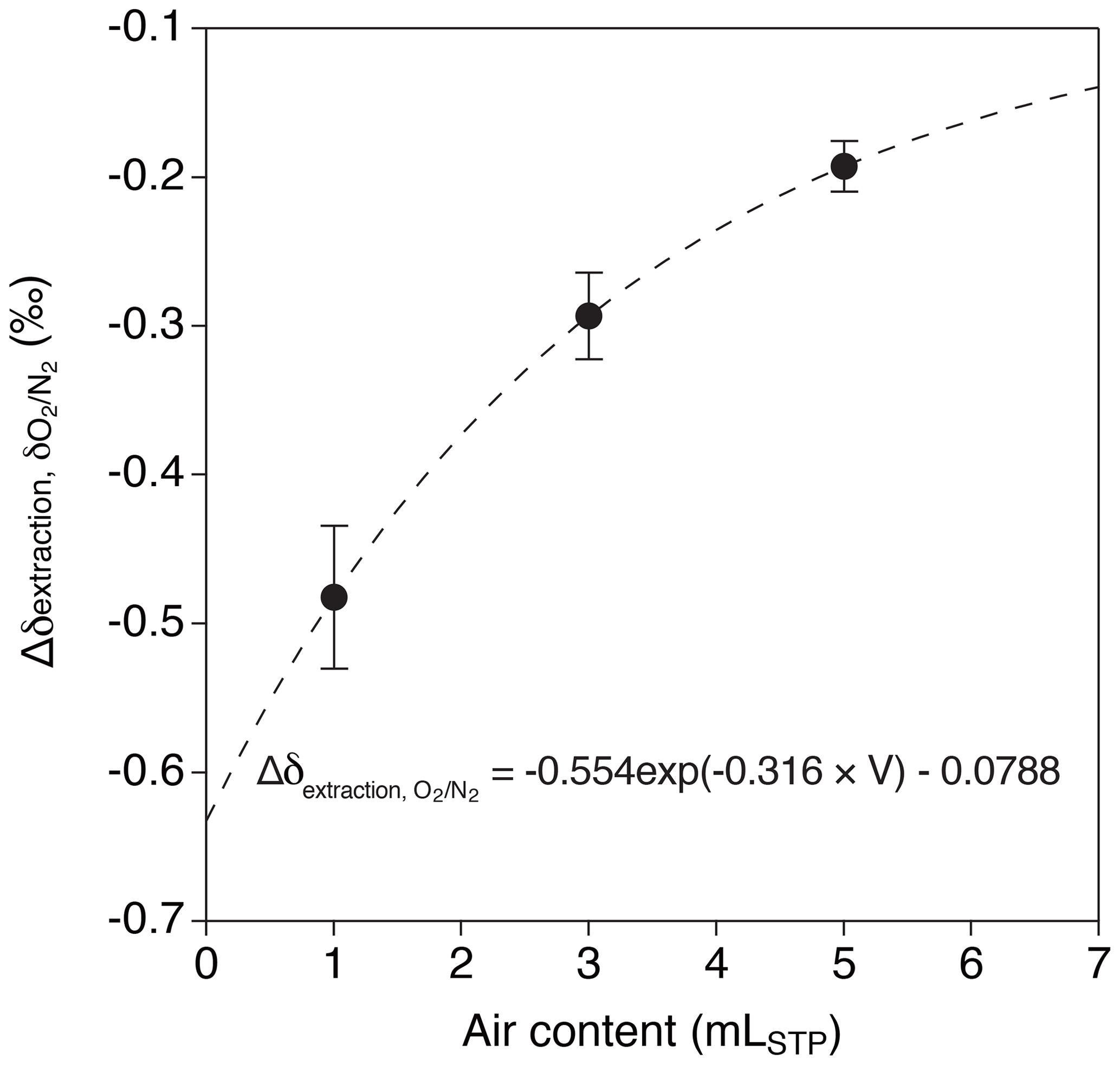
Figure 7Change of δO2∕N2 by wet extraction and overnight storage. Dashed line represents exponential fit to the data ().
4.2.3 Long-term stability of standard gas and atmosphere, and normalization of sample ratios
For normalization of the ice-core data and monitoring their long-term stability, standard gas in a cylinder (STD-A) and atmosphere (sampled outside the NIPR building) have been regularly measured against the reference can.
The atmospheric sampling and measurement procedures follow Headly (2008) and Orsi (2013). Briefly, the atmosphere is collected in a 1.5 L glass flask with a metal piston pump (Senior Aerospace, MB-158), aspirated air intake and two water traps. The flow rates of the sampling and aspiration lines are 4 and 15 L min−1, respectively, with a flushing time of > 10 min before sampling. In the laboratory, the flask air is expanded into three volumes in series (∼ 4, ∼ 1.5 and ∼ 2 mL) and allowed for 30 min to equilibrate, and the air in the middle volume is transferred to a GEPW tube. The STD-A is filled in a test tube (3 or 5 mL), and an aliquot of it (∼ 1 mLSTP) is transferred to a GEPW tube using the split line (see Sect. 4.1.2).

Figure 8Atmospheric composition measured against reference gas for (a) δ15N, (b) δ18O, (c) δO2∕N2 and (d) δAr∕N2. Open markers represent individual data points, whereas filled markers represent the means of values measured within several days (error bars are 1 SD). Grey plus (+) markers in panel (d) represent estimated δO2∕N2 of MTS-2017 against reference gas through the measurements of STD-A against the reference gas, assuming that δO2∕N2 of STD-A has not changed. Vertical grey lines indicate the timing of replacements of the reference can, and vertical light blue lines indicate the timing of filament replacements.
Table 5Composition of STD-A for mass spectrometer measurements.

δO2∕N2 is determined in July 2019 against the 2017 annual mean δO2∕N2 over Minamitorishima island provided by AIST. Other ratios are determined against outside air sampled monthly at NIPR over February 2016–December 2019.
The δ15N, δ18O, δO2∕N2 and δAr∕N2 of STD-A and atmosphere for 2016 to 2019 are shown in Figs. 6 and 8, and the values of the STD-A against the atmosphere are summarized in Table 5. Shifts in the ratios are commonly seen when the ion source filament or reference can is renewed (as indicated by vertical lines in the figure). However, there are no discernible trends and seasonal variations during the use of one reference can for all ratios except for δO2∕N2. Typical SDs of a set of atmospheric measurements (∼ 10 replicates) using two flasks within a few days are 0.003 ‰, 0.007 ‰, 0.020 ‰ and 0.034 ‰ for δ15N, δ18O, δO2∕N2, and δAr∕N2, respectively, while those of the STD-A measurements are 0.004 ‰, 0.008 ‰, 0.058 ‰ and 0.033 ‰ , respectively. Comparisons of δ15N, δ18O and δAr∕N2 between STD-A and atmosphere indicate slightly better reproducibilities for the atmospheric measurements, possibly due to fractionations during the filling of STD-A into the test tubes. Therefore, the atmosphere is the best choice for the normalization of those ratios.
General trends towards more positive values are seen for δO2∕N2 (Figs. 6d and 8d), presumably because O2 in the reference can is gradually consumed by oxidation of organic matter on the inner wall. Moreover, atmospheric δO2∕N2 in urban areas may show spikes and seasonal variations (Ishidoya and Murayama, 2014), which are much larger than our measurement precision. Indeed, δO2∕N2 of STD-A only shows linear trends (due to the drift in the reference can), but the atmospheric δO2∕N2 sometimes deviates from its linear trend by up to ∼ 0.5 ‰ (e.g., in December 2017, January 2018, April 2018, March 2019 and December 2019). Thus, the use of a standard gas in the cylinder (STD-A) for normalization, rather than the atmosphere sampled at the time of calibrations, is the better choice for precise δO2∕N2 measurements. We here define our “modern air” for δO2∕N2 as the annual average δO2∕N2 in 2017 observed over Minamitorishima island (hereafter MTS air) (24∘17′ N, 153∘59′ E) by the National Institute of Advanced Industrial Science and Technology (AIST) in cooperation with the Japan Meteorological Agency (Ishidoya et al., 2017) and determined δO2∕N2 in STD-A against it (+2.595 ‰ ± 0.008 ‰). We note that AIST recently developed a gravimetric δO2∕N2 calibration scale for precise and long-term atmospheric monitoring (Aoki et al., 2019).
In each month, the atmosphere is sampled in two flasks on the same day, and a total of 10 or more aliquots are measured and averaged. The STD-A is measured every week, and the values in the same month are averaged. The monthly atmospheric or STD-A values thus assigned against the reference can are averaged over 2 consecutive months, and the ice-core samples are normalized against the nearest 2-month-average values. The final corrected and normalized δ values of an ice-core sample are
where δATM is the 2-month-average atmospheric value against the reference can corrected for PIS and chemical slope (for effectively correcting for the drifts in the reference can).
We analyzed the Dome Fuji (hereafter DF) ice core, Antarctica, and NEEM ice core, Greenland, and compared the results with other records to evaluate the overall reliabilities of our methods. The reproducibilities of ice-core measurements are also assessed using the pooled standard deviation (SD) of duplicates (measurements of two ice samples from the same depth, Severinghaus et al., 2003) for some depths. The number of samples and depths are as follows: 49 samples from 40 depths in 112.88–157.81 m (bubbly ice, 0.2–2.0 kyr BP) and 70 samples from 35 depths in 1245.00–1918.59 m (clathrate ice, 79–150 kyr BP) from the DF core, and 74 samples from 47 depths in 112.68–449.10 m (bubbly ice and above brittle zone, 0.2–2.0 kyr BP) from the NEEM core.
Table 6Age control points for the Dome Fuji (DF) core from CH4 matching to the WAIS Divide core (WDC) (0–1800 CE)
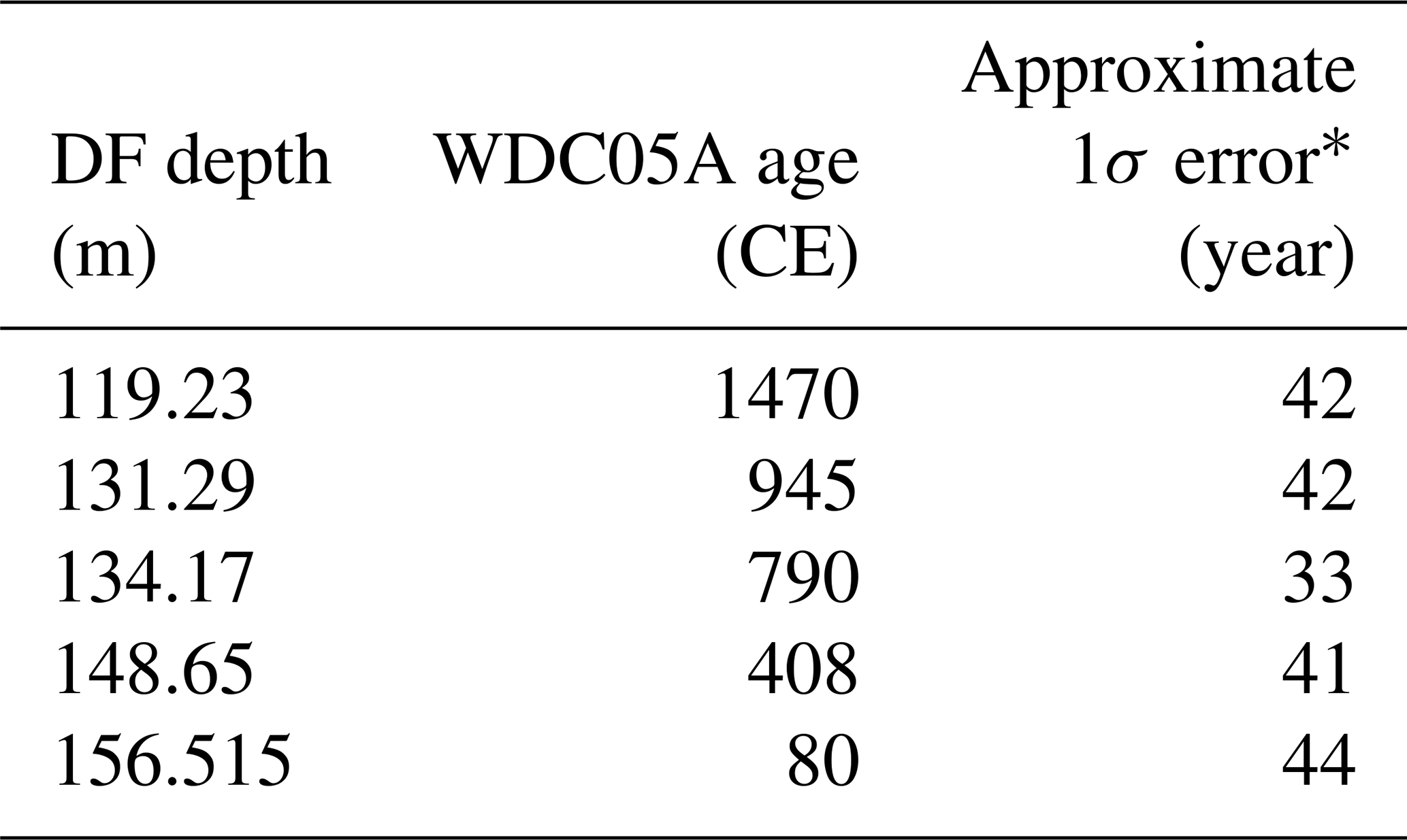
* Estimated as half of the mean age intervals from the tie point to the neighboring CH4 data points (uncertainty of WDC05A itself is also considered).
We employed the following age scales and synchronizations. For the preindustrial late Holocene (∼ 0 to ∼ 1800 CE), the GICC05 chronology was used for the NEEM core as published by Rasmussen et al. (2013), and a WAIS Divide core gas chronology (WDC05A) (Mitchell et al., 2013, 2011) was transferred to the DF core by CH4 synchronization (the tie points are shown in Fig. 10 and Table 6). For the other ice cores for comparisons (including GISP2, WDC, Law Dome cores), we employed their own published timescales (Table A1).
The following data were rejected or not acquired due to experimental errors. The DF sample at 144.75 m lost CH4, CO2, and N2O concentrations and TAC because of a connection failure between the GC and computer. δ15N, δ18O, δO2∕N2 and δAr∕N2 from the DF core at 1521.06, 1540.56 and 1712.10 m were rejected because of the leaky valve on the GEPW tube. The NEEM sample at 217.15 m showed anomalous CO2 and N2O concentrations as compared with another sample at the same depth (+83 ppm and +47 ppb, respectively); all GC data including CH4 were rejected for this sample. The NEEM sample at 229.80 and 438.83 m showed anomalously low δ15N and δ18O (half of the typical values, or lower), possibly due to gas handling error or leak. As all the anomalous NEEM data were acquired within 2 months after establishing the method, there would have been experimental errors that slipped our attention.
5.1 CH4, N2O and CO2 concentrations
The pooled SDs of the CH4, N2O and CO2 concentrations are ± 3.2 ppb, ± 1.3 ppb and ± 3.2 ppm for the DF bubbly ice (number of pairs = 8); ± 3.2 ppb, ± 2.2 ppb and ± 2.9 ppm for the DF clathrate ice (n = 28); and ± 2.9 ppb, ± 3.0 ppb and ± 5.3 ppm for the NEEM bubbly ice (n = 27) (Table 7). The pooled SDs of CH4 and N2O are similar to those reported from most precise measurements by other laboratories (± 2.8 ppb for CH4 by OSU, Mitchell et al., 2013; and ± 1.5 ppb for N2O by SNU, Ryu et al., 2018).
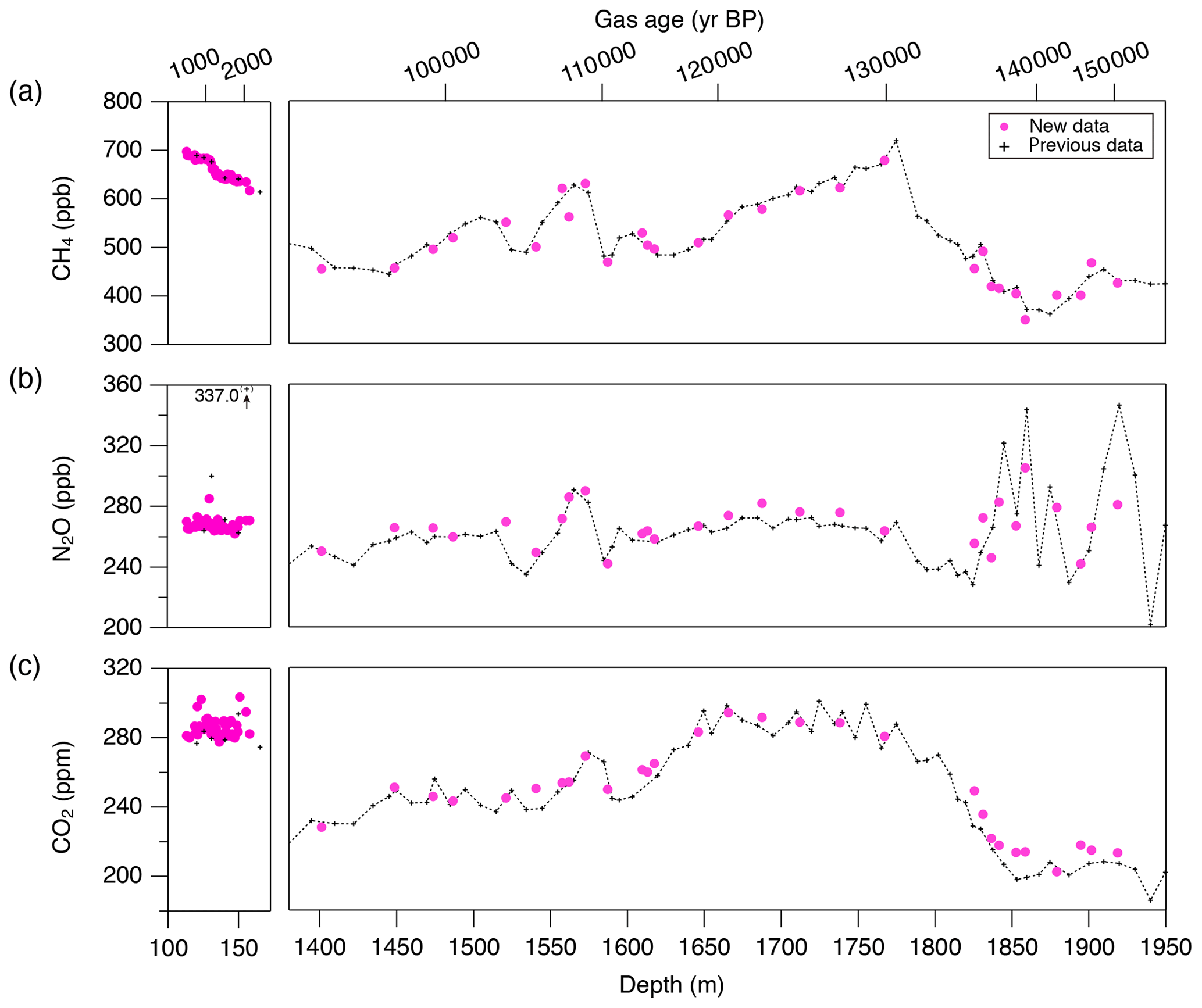
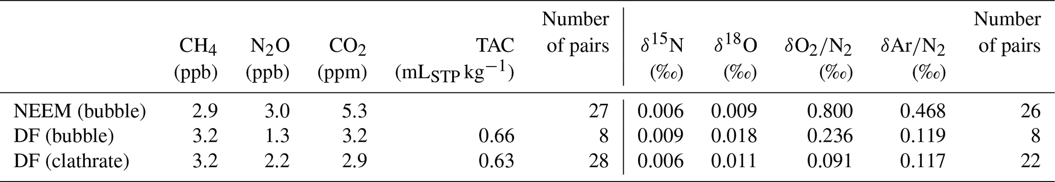
Figure 9CH4, N2O and CO2 concentrations of the Dome Fuji ice core, and comparison with previous records from the same core on the DFO-2006 gas age scale (Kawamura, 2001; Kawamura et al., 2007).

Figure 10(a) CH4, (b) N2O and (c) CO2 concentrations for 0–1800 CE from the DF and NEEM ice cores measured with our new method, and the comparison with published records (Ahn et al., 2012; Kawamura, 2001; Kawamura et al., 2007; Mitchell et al., 2013; Rubino et al., 2019; Ryu et al., 2020; Siegenthaler et al., 2005). Details are summarized in Table A1. The DF data are placed on the WDC05A chronology by placing five tie points between the CH4 variations of the DF and WD cores – thick tick marks at the bottom of panel (a), and all the other data are placed on the respective (published) timescales. Five CH4 outliers at two depths in the NEEM core, highlighted by dotted-line circles, are interpreted as natural artifacts (see text and Fig. 11).
Our new CH4, N2O and CO2 data from the DF core agree with the previous data from Tohoku University (Fig. 9) (Kawamura, 2001), indicating consistency of the TU concentration scales for ice-core analyses over the past ∼ 20 years. We compare our results for the preindustrial late Holocene (∼ 0 to 1800 CE) at ∼ 50-year resolution with other ice-core records from other groups on the NOAA concentration scales (Fig. 10). The DF CH4 data agree well with those from the WAIS Divide core by OSU (Mitchell et al., 2013) and Law Dome cores by CSIRO (Rubino et al., 2019), which are currently the best Antarctic records in terms of precision and resolution (see Fig. A1 in the Appendix for comparison with other records). We note that multi-decadal variations are smoothed out in the DF core because of the slow bubble-trapping process. For Greenland, our NEEM data show good agreement with the GISP2 data from OSU (Mitchell et al., 2013), including multi-decadal to centennial-scale variations.
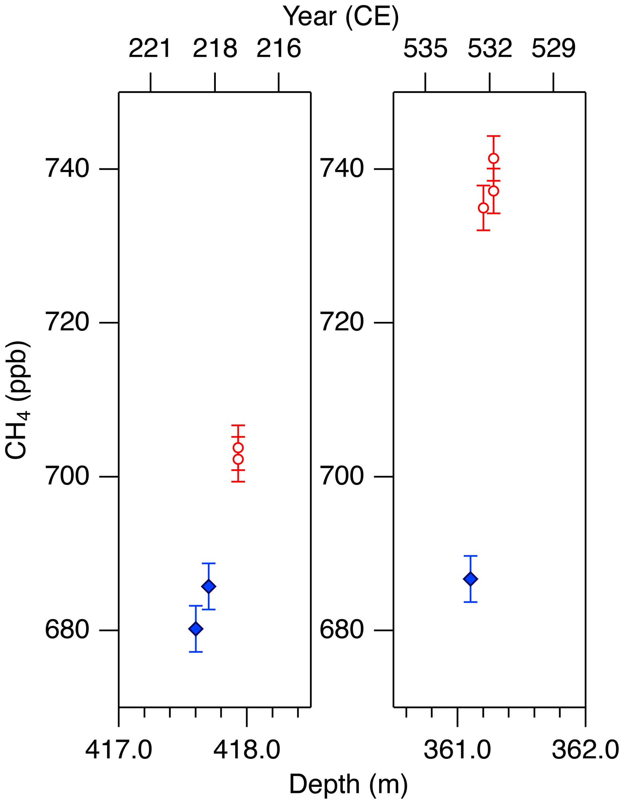
Figure 11Detailed views of individual CH4 data for the abrupt (non-atmospheric) increases in the NEEM core at ∼ 418 and 361 m. Data shown in blue agree with the GISP2 data, and those in red are unrealistically high (interpreted as natural artifacts).
We note that unrealistically high CH4 variabilities were found at two depths in the NEEM core (417.60–418.00 m and 361.05–361.35 m; gas ages are ∼ 218 and ∼ 532 CE, respectively) (Fig. 11). The change of ∼ 20 to 50 ppb between the neighboring depths (only < 1 year apart in age) is impossible to be of atmospheric origin considering diffusive mixing in firn. The good agreements between the duplicate measurements for these depths exclude the possibility of experimental failure. The N2O concentrations at the same depths are not significantly different from those in the neighboring depths, suggesting that the CH4 anomalies are not due to ice-sheet surface melt and associated gas dissolution, which should elevate both CH4 and N2O. Anomalously high CH4 concentrations with similar magnitudes have been reported from GISP2 and NEEM cores measured at other laboratories, and the reason may be CH4 production after bubble close-off (in the ice sheet) or during air extraction from dusty glacial-period ice (Mitchel et al., 2013; Rhodes et al., 2013, 2016; Lee et al., 2020). For the purpose of evaluating our system, we exclude the anomalous values from the calculation of pooled SDs and quantitative comparison with other records because they are extremely inhomogeneous. We speculate that the CH4 anomalies in our data originate in in situ production because we used the Holocene (low dust) ice, and full investigation of our system on CH4 production (as found by Lee et al., 2020) would require higher-resolution analyses of dusty ice and inter-comparison with other laboratories, which is beyond the scope of this paper. The CH4 concentration of 723.7 ppb at 961 CE (the mean of four discrete measurements), in the middle of an increase over a century, is also higher than the GISP2 data by ∼ 30 ppb, whereas the N2O concentration does not appear to be anomalous. The four discrete values agree within 12 ppb (717.6, 724.9, 729.5 and 722.9 ppb), excluding again the possibility of major experimental failure for the anomaly. This discrepancy could be due to uncertainty in age synchronization between the cores, a reversal of the NEEM gas age by firn layering (the possibility that the bubbles were closed off in the last stage of firn-ice transition, Rhodes et al., 2016) or CH4 production within the ice sheet as discussed above.
N2O concentrations from both polar regions should agree with each other within the uncertainty of ice-core analyses. Our datasets from the NEEM and DF cores agree with each other within ∼ 5 ppb without systematic bias, and they also agree with the Law Dome data by CSIRO within ∼ 5 ppb (Rubino et al., 2019). We also compare our data with the Monte Carlo spline fit through the NGRIP, TALDICE, EDML, and EDC data by the University of Bern (Fischer et al., 2019; see Fig. A1 for individual data points) and high-resolution data from the NEEM and Styx Glacier ice cores by SNU (Ryu et al., 2020). Multi-centennial-scale variations (i.e., relatively low concentrations around 600 CE and high concentrations around 1100 CE) are commonly seen in all the datasets. However, there appear to be some offsets between the data from NIPR, University of Bern and SNU. The NEEM and Styx Glacier data by SNU are systematically lower by ∼ 5 ppb than our data. Because the NEEM core is measured by both laboratories, the offset cannot be explained by the difference in the original N2O concentration in the ice. We examine here the possibility that our method overestimates the N2O concentration. Based on the standard gas transfer tests, we do not apply extraction correction for N2O concentration. This raises the possibility that, if our tests indeed underestimate the N2O dissolution, then our ice-core data should become lower than the true values. This scenario leads to an upward correction of our dataset and thus does not explain the offset. Therefore, the causes of the systematic offset between the two datasets may be the differences in standard gas scales and calibration methods employed by the two laboratories. The spline curve by the University of Bern shows the depth-dependent offset relative to other datasets. The 2σ error band of the spline curve overlaps well with our data between ∼ 1000 and 1800 CE, but it is systematically lower than our data and agrees with the SNU data for ∼ 0–1000 CE. We measure the ice samples in random order to avoid any apparent trends in the data that might originate in the drifts in the standard gases or instruments (on weekly to monthly timescales). The sample at 1076 CE (129.16 m) of the DF core shows very high concentration (∼ 20 ppb higher than the neighboring depths), which is unlikely to be due to experimental errors because the CH4 and CO2 concentrations of the same sample are not elevated. Anomalous N2O concentrations were also found in late Holocene DF samples in previous measurements (Kawamura, 2001), and they are possibly natural artifacts (N2O production in ice sheet) (Kawamura, 2001; Sowers, 2001).
The overall agreements of our CH4 and N2O data with the other datasets suggest the reliability of our method and consistency of the TU scales at low concentrations with the NOAA scales. We note that our method does not apply experimental corrections for CH4 and N2O concentrations. For reference, the OSU method (wet extraction with refreezing) applies solubility correction of 1 % (∼ 3–8 ppb) and blank correction of 2.5 ppb for CH4 (Mitchell et al., 2011), and the CSIRO method (dry extraction) applies blank corrections of 4.1 and 1.8 ppb for CH4 and N2O, respectively (MacFarling Meure et al., 2006). The negligible effect of gas dissolution in our method is explained by the immediate removal of the released air from the ice vessel, maintaining low pressure above the meltwater.
The CO2 concentration is generally measured with mechanical dry-extraction techniques (e.g., Ahn et al., 2009; Barnola et al., 1987; Monnin et al., 2001; Nakazawa et al., 1993a) and sublimation (Schmitt et al. 2011), because the wet-extraction method has a risk of contamination by acid–carbonate reaction and oxidation of organic materials in meltwater. While CO2 production in the meltwater indeed occurs, its magnitude is up to 20 ppm, and the glacial-interglacial CO2 variations are well captured in the DF record for the last 340 kyr BP (Kawamura et al., 2003). Our new wet-extraction CO2 values of the DF core for the last 2000 years agree with the Law Dome (MacFarling Meure et al., 2006), EDML (Siegenthaler et al., 2005) and WAIS Divide (Ahn et al., 2012) ice cores mostly within 0 to +10 ppm, with several ∼ 20 ppm deviations. The NEEM wet-extraction CO2 data are higher than those of DF and other ice cores by ∼ 10–30 ppm (maximum ∼ 60 ppm), which is much larger than the pooled SD (5.3 ppm for the NEEM dataset). This result is not surprising because it is well known that reliable CO2 reconstructions are only possible from Antarctic ice cores owing to in situ CO2 production in the Greenland ice sheet with high impurity concentrations (Anklin et al., 1995). Anklin et al. (1995) measured Eurocore (Greenland) late Holocene ice with both dry- and wet-extraction methods and found that the wet-extraction values were higher (by ∼ 30 to 100 ppm) than the dry-extraction values, which in turn are higher than the Antarctic records by up to ∼ 20 ppm. Their results thus suggest that the excess CO2 in our NEEM dataset might be partly produced during the extraction by chemical reactions in the meltwater.
5.2 Elemental and isotopic compositions of N2, O2 and Ar
5.2.1 Gas-loss fractionation and surface removal
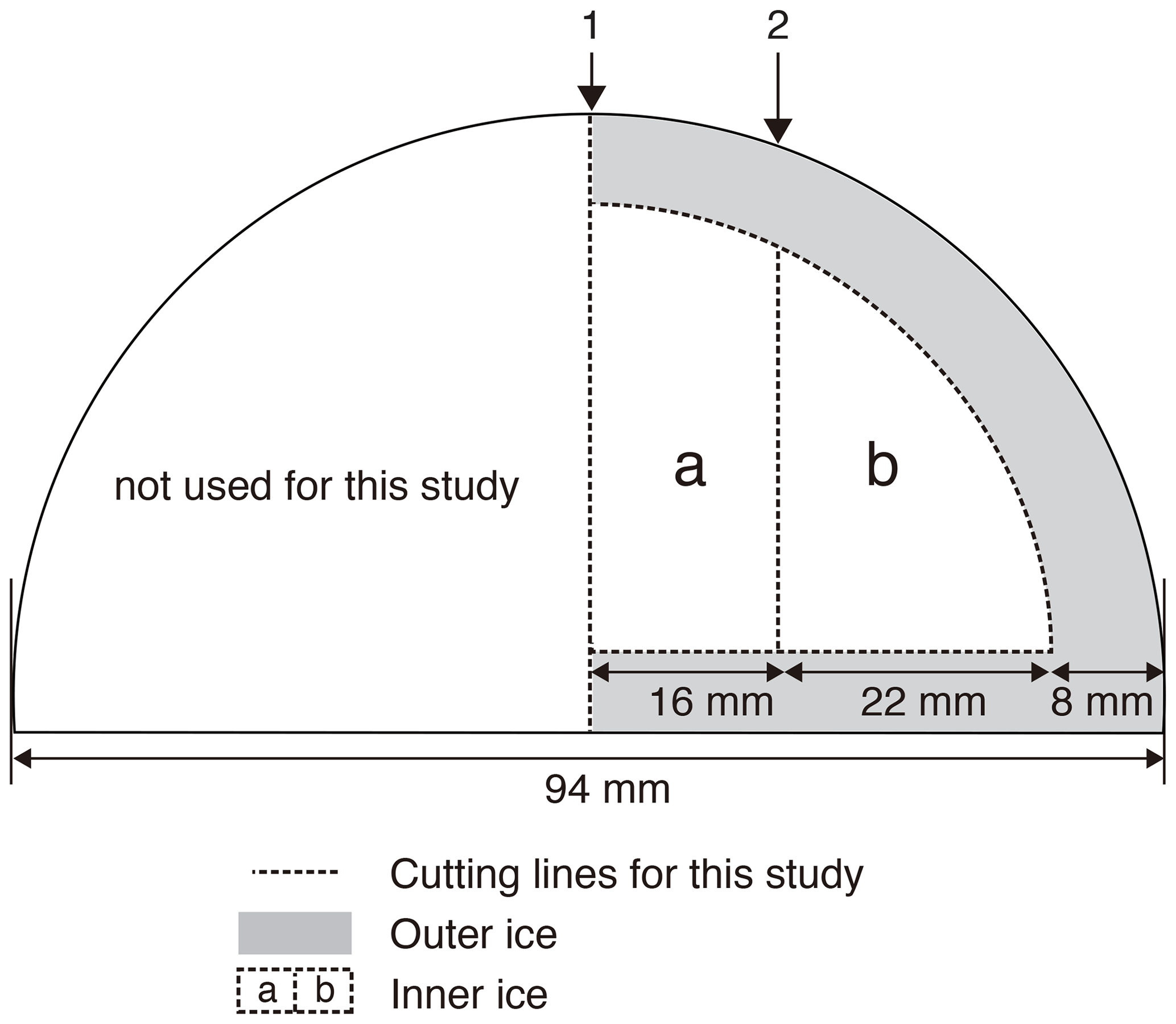
Figure 12Typical cross-sectional cutting plan of the DF core for duplicate measurements and outer–inner comparisons for mass spectrometer analyses. The sample length is ∼ 12 cm. The original outer surface (black line) has been exposed to the atmosphere for ∼ 20 years. The ice is first cut at line 1, then the outer part is removed, and finally the inner ice is cut at line 2 into “a” and “b” pieces. Dashed lines indicate the boundaries between “a,” “b,” and “outer” pieces. For a single (non-duplicate) measurement, the ice is not cut at line 1 (only cut at line 2 to produce the “b” piece).
Previous studies have indicated that gases can slightly be lost from ice cores during storage, causing size- and mass-dependent fractionations in δO2∕N2, δ18O and δAr∕N2 (Bender et al., 1995; Bereiter et al., 2009; Huber et al., 2006a; Ikeda-Fukazawa et al., 2005; Kawamura et al., 2007; Severinghaus et al., 2009). Greenhouse gas concentrations could also be biased (presumably to higher values, Ikeda-Fukazawa et al., 2004, 2005; Bereiter et al., 2009; Eggleston et al. 2016), but they would not be detected in most cases with the current measurement precision. As the δO2∕N2, δ18O and δAr∕N2 ratios become fractionated especially in the exposed outer part of the core, the surface must sufficiently be removed to precisely measure the air composition and accurately reconstruct the ratios as originally archived in the ice sheet (Bereiter et al., 2009; Ikeda-Fukazawa et al., 2005; Kawamura et al., 2007; Severinghaus et al., 2009). The thickness of sufficient surface removal should depend on the storage period, storage temperature and the form of air in ice (bubbles or clathrate hydrates). To examine whether those ratios as originally recorded in the ice sheet can be found in the long-stored DF core (at −50 ∘C for ∼ 20 years), we measured samples from the same depths with different thickness of surface removal (e.g., 8 and 5 mm) (Fig. 12). The outer ice pieces were also measured, and the results were compared with those from the inner ice.
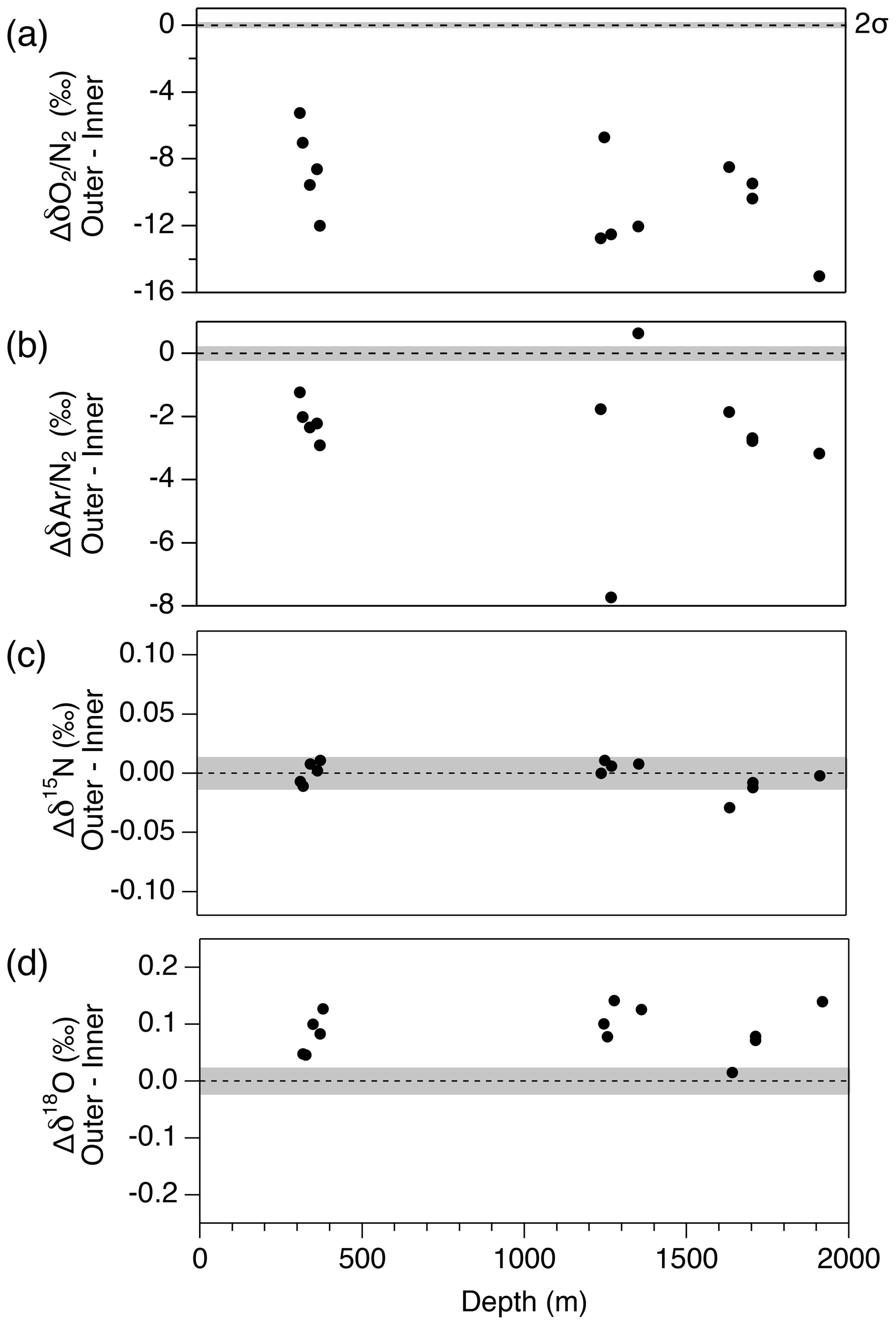
Figure 13Pair difference (Δ) between outer ice and inner ice for (a) δO2∕N2, (b) δAr∕N2, (c) δ15N and (d) δ18O. Grey shadings indicate the estimated 2σ uncertainty for clathrate ice (from pooled SDs of duplicates with > 8 mm of outer removal).
First, we compare the data from the outer ice and inner ice to validate the magnitude of gas-loss fractionation. For both the bubbly ice and clathrate ice (note that bubble–clathrate transition zone is not investigated), all the measured samples show lower δO2∕N2 and δAr∕N2 in the outer ice than those in the inner ice (Fig. 13). In addition, δO2∕N2 is more depleted than δAr∕N2, consistent with the gas-loss fractionations found in earlier studies, which proposed that the gas-loss fractionation is largely size dependent (molecular diameter of O2 is smaller than Ar) with weak mass dependency (Bender et al., 1995; Huber et al., 2006a; Severinghaus et al., 2009). Most samples show higher δ18O in the outer ice than in the inner ice. In contrast, δ15N from the outer and inner ice agree with each other, suggesting that detectable mass-dependent fractionation occurred for O2, but not for N2, via the gas loss from the outer ice.

Figure 14Pair difference between the two inner ice pieces with the thickness of outer removal of 5 and 8 mm for (a) δO2∕N2, (b) δAr∕N2, (c) δ15N and (d) δ18O. Grey shadings indicate the estimated 2σ uncertainty for clathrate ice (from pooled SDs of duplicates with > 8 mm of outer removal).
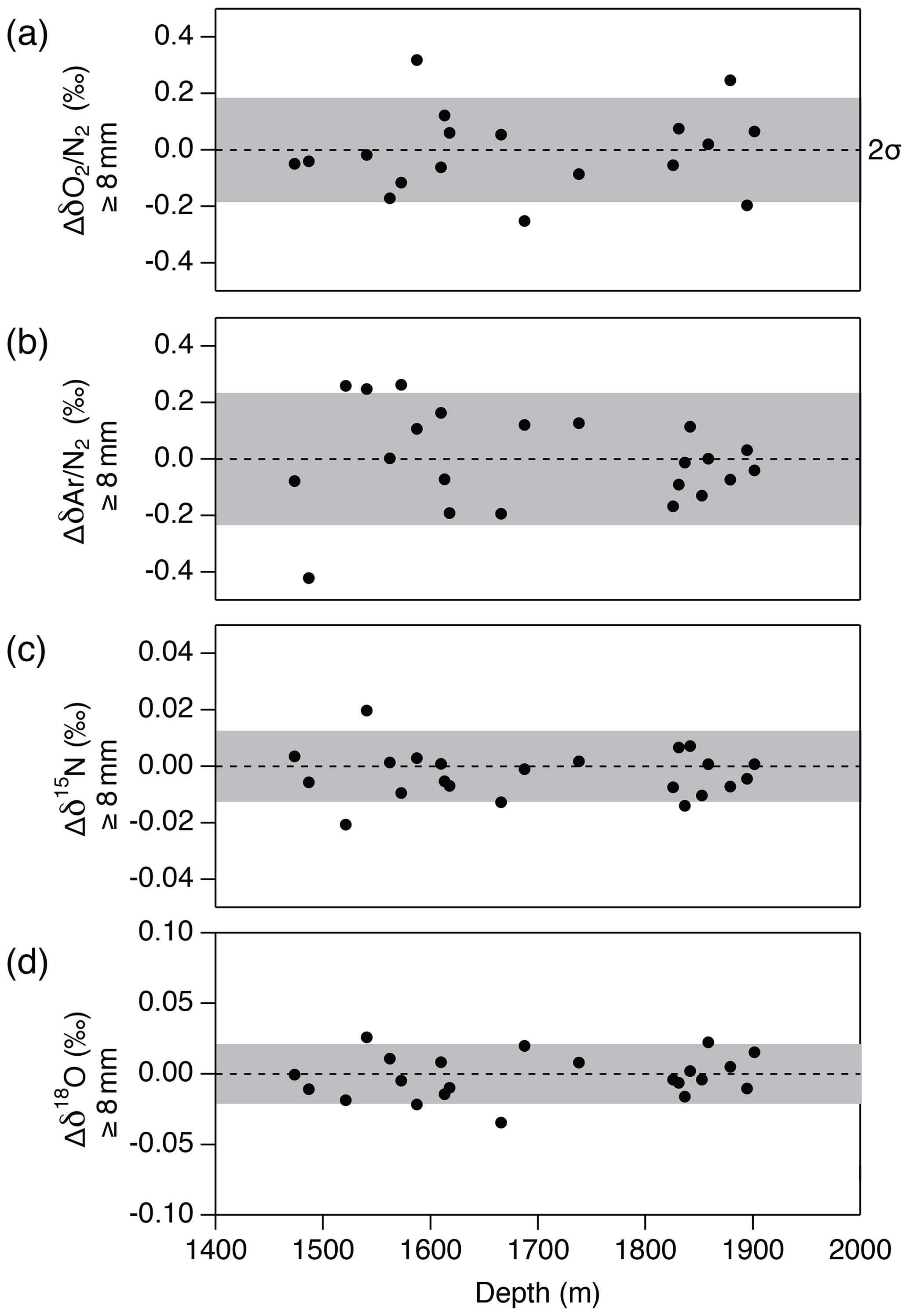
Figure 15Pair difference between the two inner ice pieces (data from the “b” piece minus that from the “a” piece) whose outer parts are removed by 8 mm or more for (a) δO2∕N2, (b) δAr∕N2, (c) δ15N and (d) δ18O. Grey shadings indicate the estimated 2σ uncertainty for clathrate ice (from pooled SDs of duplicates).
Next, we examine the δO2∕N2 data from the inner ice with different thicknesses of surface removal. Below 1380 m (pure clathrate ice), the δO2∕N2 values from the inner ice with the outer removal of 5 mm are mostly lower than those from the adjacent pieces with 8 mm removal (Fig. 14), suggesting that gas loss affects the gas composition to more than 5 mm from the surface. On the other hand, no significant differences are observed between δO2∕N2 values from the inner ice (with different outer removal) if the removal is 8 mm or more (we tested with combinations of 8, 9, 11 and 13 mm) (Fig. 15). The δAr∕N2, δ15N and δ18O data from the inner ice with surface removal of 5 and 8 mm are not different from each other, suggesting insignificant mass-dependent gas-loss fractionation in ice > 5 mm away from the surface. From these results, we conclude that the removal of 8 mm is sufficient to obtain the gas composition as originally trapped in the DF1 core. For our routine measurements of the DF core, we decided to cut 9 mm to include an extra margin.
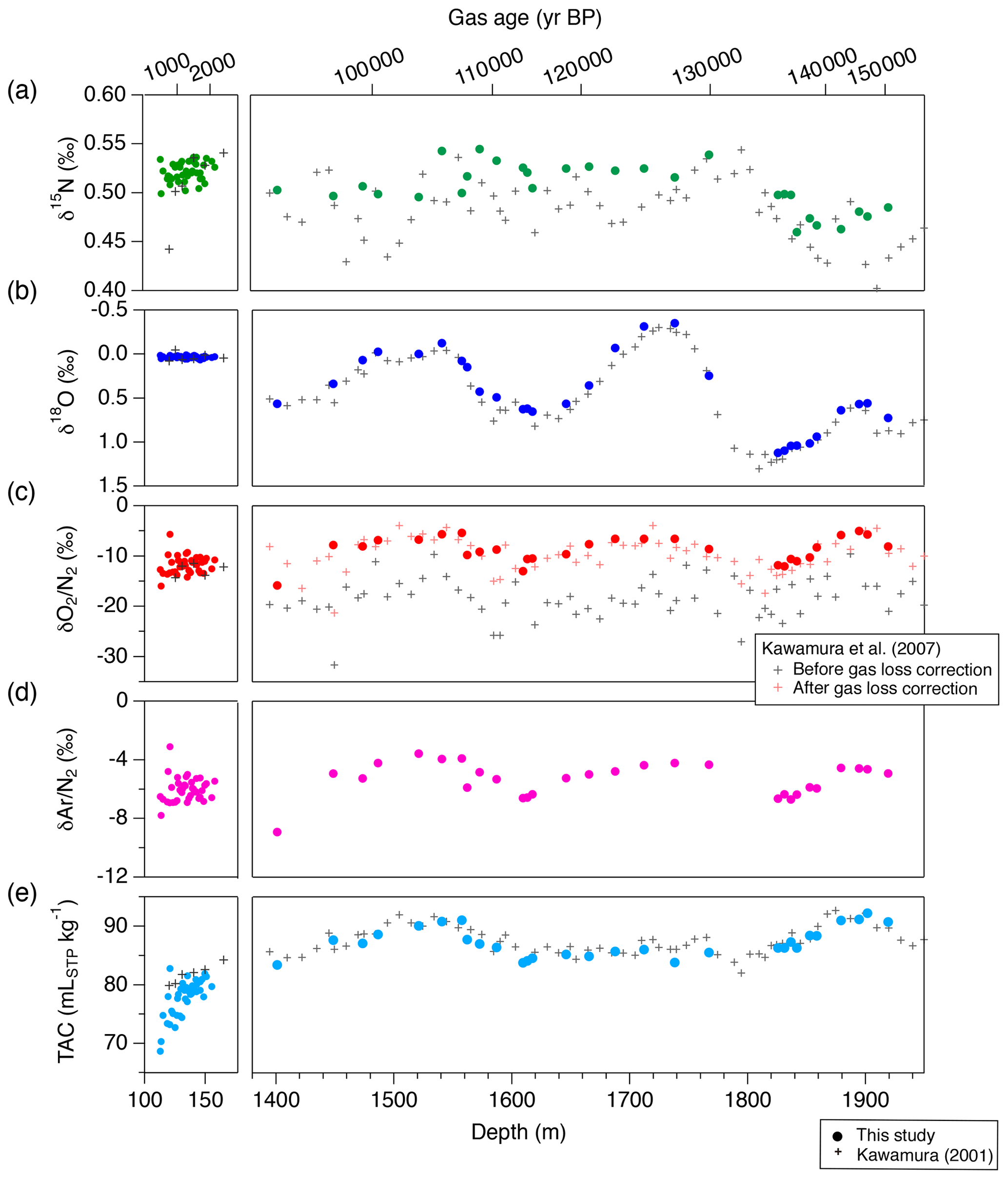
Figure 16The DF records of mass spectrometer measurements and TAC from this study (filled markers), and comparison with previous records from the same core on the DFO-2006 gas age scale (crosses, Kawamura, 2000; Kawamura et al., 2007). (a) δ15N, (b) δ18O, (c) δO2∕N2, (d) δAr∕N2 and (e) TAC. For the previous δO2∕N2 records in the right subpanel of panel (c), both raw data (black) and corrected data for gas-loss fractionation during core storage at −25 ∘C (red) are shown.
5.2.2 Reproducibility and comparison with previous data
The pooled SDs for the DF clathrate hydrate ice with removal thickness of > 8 mm are 0.006 ‰, 0.011 ‰, 0.091 ‰ and 0.117 ‰ for δ15N, δ18O, δO2∕N2 and δAr∕N2, respectively (Table 7). The reproducibility of δO2∕N2 is 1 order of magnitude better than those previously reported (Bender, 2002; Extier et al., 2018). The reproducibilities for δ15N and δ18O are comparable to but slightly worse than the most precise measurements by SIO (Seltzer et al., 2017; Severinghaus et al., 2009).
We compare our new DF data with previous data from Tohoku University (Fig. 16) (Kawamura, 2001; Kawamura et al., 2007). The previous δO2∕N2 data were significantly depleted due to gas loss during the sample storage at −25 ∘C (Fig. 16c, grey marks); thus they were corrected for effect by assuming a linear relationship between the storage duration and δO2∕N2 (Fig. 16c, red marks). Our new δO2∕N2 data agree with the gas-loss-corrected old data, suggesting that δO2∕N2 as originally trapped in the DF core can be reconstructed from the 20-year-old samples and that the relatively large gas-loss correction by Kawamura et al. (2007) was rather accurate. The new δ15N and δ18O data generally agree with those of Kawamura (2001) and Kawamura et al. (2007) within the uncertainty of the old data, although the large uncertainties of the old datasets do not permit precise comparisons.
The duplicate measurements of bubbly ice of the NEEM core (by removing more than 3 mm from the surface) produced pooled SDs for δ15N and δ18O (0.006 ‰ and 0.009 ‰) similar to those for the DF clathrate ice (Table 7). This suggests that the removal of 3 mm is sufficient for the bubbly ice at least for the isotopic ratios, possibly due to generally low pressure of bubbly ice (because it is shallower) compared with clathrate ice. On the other hand, pooled SDs for δO2∕N2 and δAr∕N2 of the bubble ice are much larger than those for the DF clathrate ice (0.236 ‰ and 0.119 ‰ for the DF core, and 0.800 ‰ and 0.468 ‰ for the NEEM core, respectively), possibly related to the natural variability of pressure and composition of individual air bubbles with different trapping histories (Ikeda-Fukazawa et al., 2001; Kobashi et al., 2015). The larger pooled SDs for the NEEM core than those of the DF core possibly reflect the natural difference within the ice sheets or artifacts (gas loss) during drilling, handling and storage at the NEEM site associated with the warmer environment compared to the Dome Fuji drilling site. We also note that, due to the small number of duplicates for the bubbly ice, it is difficult at this stage to assess whether there is small systematic lowering of δO2∕N2 and δAr∕N2 with the 3 mm removal.
5.3 Total air content
The pooled SDs for TAC are 0.66 and 0.67 mLSTP kg−1 for both DF bubbly ice and clathrate ice. The data from the clathrate ice agree with those from previous measurements using ∼ 300 g of ice (Kawamura, 2001), while the data from the bubbly ice appear to be lower than the previous data, especially for the shallowest depths (Fig. 16). These results may be explained by the fact that TAC of bubbly ice is biased towards lower values due to the so-called “cut-bubble effect” (Martinerie et al., 1990), in which bubbles intersecting the sample surfaces are cut and lose air. The cut-bubble effect is larger for samples with a smaller surface-to-volume ratio and samples from shallower depths.
We presented a new analytical technique for high-precision, simultaneous measurements of CH4, N2O and CO2 concentrations; isotopic and elemental ratios of N2, O2 and Ar; and total air content from a single ice-core sample with relatively small size (50–70 g) by a wet extraction. The ice sample is melted under a vacuum in 3 min, and the released air is continuously transferred and cryogenically trapped into a sample tube, with the total duration for extraction of about 10 min. The rapid and continuous transfer minimizes contaminations due to degassing from the inner walls of the apparatus, as well as dissolution of the sample air into the meltwater. The extracted air is homogenized in the sample tube for one night and split into two aliquots for mass spectrometric measurement (∼ 20 % of the sample) and gas chromatographic measurement (∼ 80 % of the sample).
The system performance was evaluated by measuring the standard gas after treating it as the ice-core air extraction, by passing it through the extraction and split lines with gas-free water in the extraction vessel. We do not observe significant changes in the mean CH4, N2O and CO2 concentrations, possibly because of the long evacuation, rapid and continuous gas transfer at low pressure over meltwater, and passivation treatments of the extraction lines and sample tubes. Thus, we do not apply corrections (e.g., so-called blank correction and solubility correction) for the greenhouse gas concentrations. For the mass spectrometry, we do not observe significant changes in δ18O, while we observe changes in δ15N, δO2∕N2 and δAr∕N2. Moreover, the change in δO2∕N2 is dependent on the sample size. Thus, we apply constant corrections for δ15N and δAr∕N2, as well as sample-size-dependent correction for δO2∕N2.
SDs of duplicate measurements for DF clathrate ice are 3.2 ppb, 2.2 ppb, and 2.9 ppm for CH4, N2O and CO2 concentrations, respectively, and 0.006 ‰, 0.011 ‰, 0.09 ‰ and 0.12 ‰ for δ15N, δ18O, δO2∕N2 and δAr∕N2, respectively. The CH4 and N2O data from the DF and NEEM ice cores for the last 2000 years agree well with those from the GISP2, WAIS Divide and Law Dome cores. We also demonstrate significant gas-loss-induced depletion of δO2∕N2 in the ice near the sample surface of the DF clathrate ice, which has been stored at −50 ∘C over ∼ 20 years. The original δO2∕N2, δAr∕N2, δ15N and δ18O in the ice sheet may still be obtained by removing the sample surface by > 8 mm.
Our new method will have many paleoclimatic applications, such as detecting subtle variations in greenhouse gas cycles (in particular CH4 inter-polar difference and N2O variations), hydrological cycles (δ18O of O2), insolation signals for dating (δO2∕N2 and δAr∕N2), and local climatic and glaciological conditions (δ15N and TAC) from deep ice cores with high temporal resolution.
Table A1Ice cores and timescales shown in this study.

* Offset correction was made to CH4 concentrations by following Beck et al. (2018).
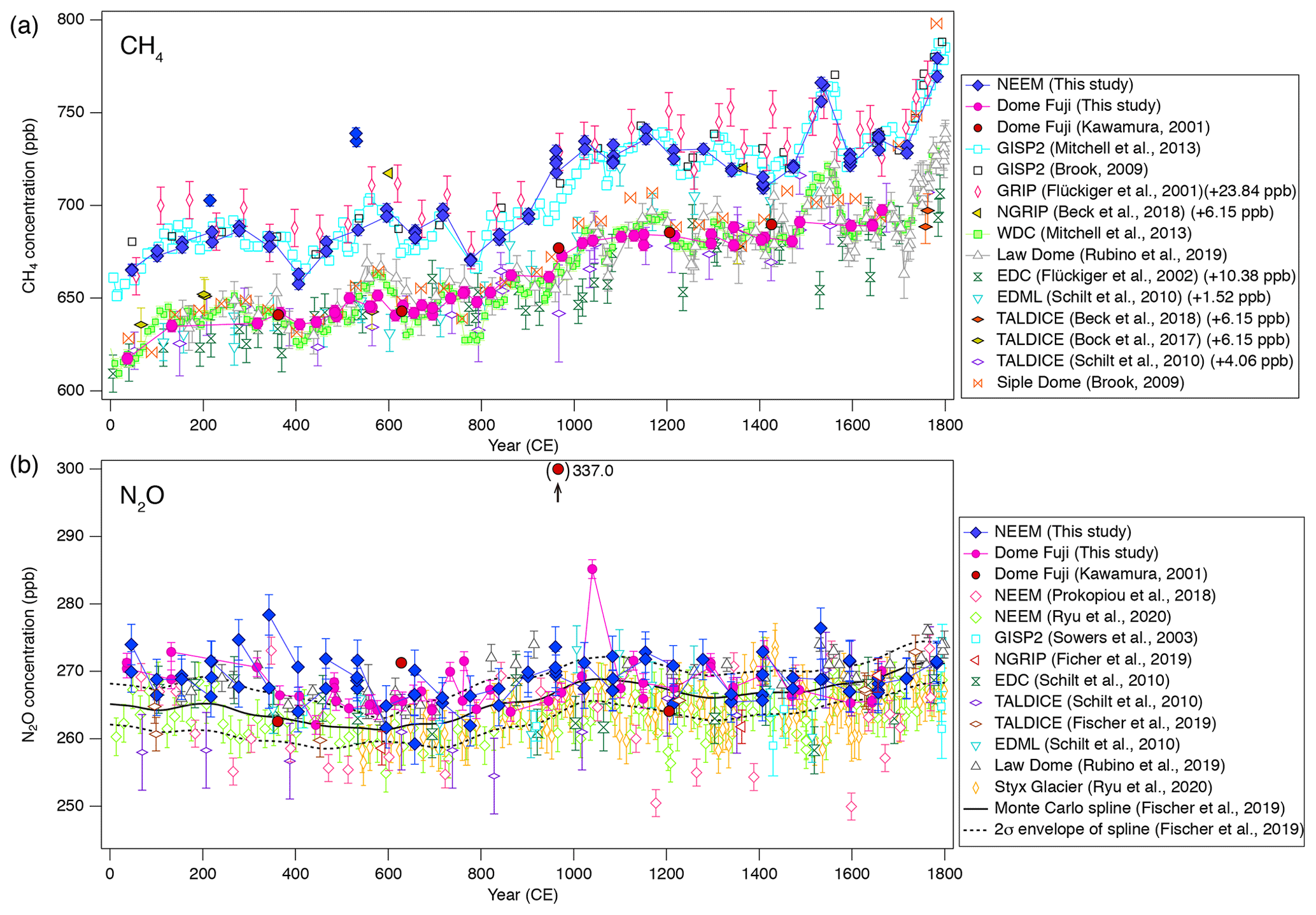
Figure A1(a) CH4 and (b) N2O concentrations for 0–1800 CE from the DF and NEEM ice cores measured with our new method, and the comparison with published records from other groups (Beck et al., 2018; Bock et al., 2017; Brook, 2009; Fischer et al., 2019; Flückiger et al., 2002; Kawamura, 2001; Mitchell et al., 2013; Prokopiou et al., 2018; Rubino et al., 2019; Ryu et al., 2020; Schilt et al., 2010; Sowers et al., 2003). The DF data are placed on the WDC05A chronology (see Fig. 10), and all the other data are placed on the respective (published) timescales (details are summarized in Table A1). The GRIP, NGRIP, EDC, EDML and TALDICE data are corrected for systematic offsets relative to the WDC data, as reported by Beck et al. (2018).
Gas data of the Dome Fuji and NEEM ice cores are available at the NIPR ADS data repository (https://doi.org/10.17592/001.2020050101; Oyabu et al., 2020) and will be available on the NOAA paleoclimate database.
The supplement related to this article is available online at: https://doi.org/10.5194/amt-13-6703-2020-supplement.
KeK designed the wet-extraction apparatus and mass spectrometer configuration and developed the overall concept of the splitting and multiple-species analyses. KeK, SS and AK designed the GC configurations. JPS and RB developed the calibration protocols for atmospheric normalization of mass spectrometer measurements except for δO2∕N2 and customized ISODAT scripts. AO designed the split line. RD developed GC controlling software with a discussion with KeK. SI provided the δO2∕N2 standard scale. DDJ provided the NEEM ice-core samples. KGA provided funding for the mass spectrometer and the NEEM samples as the national representative. SA and TN provided the greenhouse gas concentration scales and funding for the wet-extraction apparatus and cryostat. IO and KyK made the measurements. IO, KyK and KeK established the detailed procedures of ice-core measurements and calibrations. CS contributed to the early stages of development. IO and KeK wrote the manuscript, and all authors contributed to the discussion.
The authors declare that they have no conflict of interest.
We thank Yumiko Miura for a part of the data reduction; Akito Tanaka, Satoko Nakanishi, Mariko Hayakawa and Satomi Oda for the measurements; and Shinji Morimoto for providing the Tohoku University scales and assisting our standard gas calibrations. We acknowledge the Dome Fuji drilling projects led by Okitsugu Watanabe, Yoshiyuki Fujii, and Hideaki Motoyama and participants in the Japanese Antarctic Research Expedition and Ice Core Consortium related to the Dome Fuji fieldwork and management. NEEM is directed and organized by the Center of Ice and Climate at the Niels Bohr Institute and US NSF, Office of Polar Programs. It is supported by funding agencies and institutions in Belgium (FNRS-CFB and FWO), Canada (NRCan/GSC), China (CAS), Denmark (FIST), France (IPEV, CNRS/INSU, CEA and ANR), Germany (AWI), Iceland (RannIs), Japan (NIPR), Korea (KOPRI), the Netherlands (NWO/ALW), Sweden (VR), Switzerland (SNF), the United Kingdom (NERC), and the USA (US NSF, Office of Polar Programs). This study was supported by the Japan Society for the Promotion of Science (JSPS) and the Ministry of Education, Culture, Sports, Science and Technology of Japan (MEXT) KAKENHI grant numbers 17K12816, 17J00769 and 20H04327 to Ikumi Oyabu; 20H00639, 17H06316, 15KK0027, 26241011, 21671001 and 18749002 to Kenji Kawamura; 22221002 to Kumiko Goto-Azuma; 18K01129 to Shigeyuki Ishidoya; and 22310003 to Takakiyo Nakazawa. SA was supported by the GRENE Arctic Climate Change Research Project of MEXT. Shigeyuki Ishidoya was supported by the Global Environment Research Coordination System from the Ministry of the Environment. This study was also supported by Project Research KP305 and the Senshin Project from the National Institute of Polar Research and partially carried out in the Arctic Challenge for Sustainability II (ArCS II), program grant number JPMXD1420318865. We are grateful for constructive comments, remarks and advice from Jochen Schmitt and an anonymous reviewer.
This research has been supported by the JSPS KAKENHI (grant nos. 17K12816, 17J00769, 20H04327, 20H00639, 15KK0027, 26241011, 21671001, 18749002, 22221002, 18K01129 and 22310003); the Ministry of Education, Culture, Sports, Science and Technology of Japan (grant no. 17H06316 and GRENE Arctic Climate Change Research Project, Arctic Challenge for Sustainability II (ArCS II), program grant number JPMXD1420318865); the Ministry of the Environment of Japan (Global Environment Research Coordination System); and the National Institute of Polar Research (grant no. KP305 and Senshin Project).
This paper was edited by Frank Keppler and reviewed by Jochen Schmitt and one anonymous referee.
Ahn, J., Brook, E. J., and Howell, K.: A high-precision method for measurement of paleoatmospheric CO2 in small polar ice samples, J. Glaciol., 55, 499–506, https://doi.org/10.3189/002214309788816731, 2009.
Ahn, J., Brook, E. J., Mitchell, L., Rosen, J., McConnell, J. R., Taylor, K., Etheridge, D., and Rubino, M.: Atmospheric CO2 over the last 1000 years: A high-resolution record from the West Antarctic Ice Sheet (WAIS) Divide ice core, Global Biogeochem. Cy., 26, https://doi.org/10.1029/2011GB004247, 2012.
Anklin, M., Barnola, J. M., Schwander, J., Stauffer, B., and Raynaud, D.: Processes Affecting the CO2 Concentrations Measured in Greenland Ice, Tellus B, 47, 461–470, https://doi.org/10.1034/j.1600-0889.47.issue4.6.x, 1995.
Aoki, N., Ishidoya, S., Matsumoto, N., Watanabe, T., Shimosaka, T., and Murayama, S.: Preparation of primary standard mixtures for atmospheric oxygen measurements with less than 1 µmol mol−1 uncertainty for oxygen molar fractions, Atmos. Meas. Tech., 12, 2631–2646, https://doi.org/10.5194/amt-12-2631-2019, 2019.
Aoki, S., Nakazawa, T., Murayama, S., and Kawaguchi, S.: Measurements of atmospheric methane at the Japanese Antarctic Station, Syowa, Tellus, 44, 273–281, https://doi.org/10.3402/tellusb.v44i4.15455, 1992.
Barnola, J. M., Raynaud, D., Korotkevich, Y. S., and Lorius, C.: Vostok Ice Core Provides 160,000-Year Record of Atmospheric CO2, Nature, 329, 408–414, https://doi.org/10.1038/329408a0, 1987.
Bazin, L., Landais, A., Lemieux-Dudon, B., Toyé Mahamadou Kele, H., Veres, D., Parrenin, F., Martinerie, P., Ritz, C., Capron, E., Lipenkov, V., Loutre, M.-F., Raynaud, D., Vinther, B., Svensson, A., Rasmussen, S. O., Severi, M., Blunier, T., Leuenberger, M., Fischer, H., Masson-Delmotte, V., Chappellaz, J., and Wolff, E.: An optimized multi-proxy, multi-site Antarctic ice and gas orbital chronology (AICC2012): 120–800 ka, Clim. Past, 9, 1715–1731, https://doi.org/10.5194/cp-9-1715-2013, 2013.
Beck, J., Bock, M., Schmitt, J., Seth, B., Blunier, T., and Fischer, H.: Bipolar carbon and hydrogen isotope constraints on the Holocene methane budget, Biogeosciences, 15, 7155–7175, https://doi.org/10.5194/bg-15-7155-2018, 2018.
Bender, M., Sowers, T., and Lipenkov, V.: On the concentrations of O2, N2, and Ar in trapped gases from ice cores, J. Geophys. Res., 100, 18651–18660, https://doi.org/10.1029/94JD02212, 1995.
Bender, M. L.: Orbital tuning chronology for the Vostok climate record supported by trapped gas composition, Earth Planet. Sc. Lett., 204, 275–289, https://doi.org/10.1016/S0012-821X(02)00980-9, 2002.
Bereiter, B., Schwander, J., Luthi, D., and Stocker, T. F.: Change in CO2 concentration and O2∕N2 ratio in ice cores due to molecular diffusion, Geophys. Res. Lett., 36, L05703–05705, https://doi.org/10.1029/2008GL036737, 2009.
Bereiter, B., Kawamura, K., and Severinghaus, J. P.: New methods for measuring atmospheric heavy noble gas isotope and elemental ratios in ice core samples, Rapid Commun. Mass Sp., 32, 801–814, doi/10.1002/rcm.8099, 2018.
Blunier, T. and Brook, E. J.: Timing of millennial-scale climate change in Antarctica and Greenland during the last glacial period, Science, 291, 109–112, https://doi.org/10.1126/science.291.5501.109, 2001.
Blunier, T., Chappellaz, J., Schwander, J., Stauffer, B., and Raynaud, D.: Variations in atmospheric methane concentration during the Holocene epoch, Nature, 374, 46–49, https://doi.org/10.1038/374046a0, 1995.
Bock, M., Schmitt, J., Beck, J., Schneider, R., and Fischer, H.: Improving accuracy and precision of ice core δD(CH4) analyses using methane pre-pyrolysis and hydrogen post-pyrolysis trapping and subsequent chromatographic separation, Atmos. Meas. Tech., 7, 1999–2012, https://doi.org/10.5194/amt-7-1999-2014, 2014.
Bock, M., Schmitt, J., Beck, J., Seth, B., Chappellaz, J., and Fischer, H.: Glacial/interglacial wetland, biomass burning, and geologic methane emissions constrained by dual stable isotopic CH4 ice core records, P. Natl. Acad. Sci. USA, 114, E5778–E5786, https://doi.org/10.1073/pnas.1613883114, 2017.
Brook, E. J.: Methane measurements from the GISP2 and Siple Dome ice cores, U.S. Antarctic Program (USAP) Data Center, https://doi.org/10.7265/N58P5XFZ, 2009.
Brook, E. J., Sowers, T., and Orchardo, J.: Rapid variations in atmospheric methane concentration during the past 110,000 years, Science, 273, 1087–1091, https://doi.org/10.1126/science.273.5278.1087, 1996.
Brook, E. J., White, J. W. C., Schilla, A. S. M., Bender, M. L., Barnett, B., Severinghaus, J. P., Taylor, K. C., Alley, R. B., and Steig, E. J.: Timing of millennial-scale climate change at Siple Dome, West Antarctica, during the last glacial period, Quaternary Sci. Rev., 24, 1333–1343, https://doi.org/10.1016/j.quascirev.2005.02.002, 2005.
Buizert, C., Cuffey, K. M., Severinghaus, J. P., Baggenstos, D., Fudge, T. J., Steig, E. J., Markle, B. R., Winstrup, M., Rhodes, R. H., Brook, E. J., Sowers, T. A., Clow, G. D., Cheng, H., Edwards, R. L., Sigl, M., McConnell, J. R., and Taylor, K. C.: The WAIS Divide deep ice core WD2014 chronology – Part 1: Methane synchronization (68–31 ka BP) and the gas age–ice age difference, Clim. Past, 11, 153–173, https://doi.org/10.5194/cp-11-153-2015, 2015.
Chappellaz, J., Blunier, T., Kints, S., Dällenbach, A., Barnola, J.-M., Schwander, J., Raynaud, D., and Stauffer, B.: Changes in the atmospheric CH4 gradient between Greenland and Antarctica during the Holocene, J. Geophys. Res., 102, 15987–15997, https://doi.org/10.1029/97JD01017, 1997.
Chappellaz, J. A., Fung, I. Y., and Thompson, A. M.: The atmospheric CH4 increase since the Last Glacial Maximum, Tellus, 45, 228–241, https://doi.org/10.3402/tellusb.v45i3.15726, 1993.
Dlugokencky, E. J.: Conversion of NOAA atmospheric dry air CH4 mole fractions to a gravimetrically prepared standard scale, J. Geophys. Res., 110, https://doi.org/10.1029/2005JD006035, 2005.
Eggleston, S., Schmitt, J., Bereiter, B., Schneider, R., and Fischer, H.: Evolution of the stable carbon isotope composition of atmospheric CO2 over the last glacial cycle, Paleoceanography, 31, 434–452, https://doi.org/10.1002/2015PA002874, 2016.
Extier, T., Landais, A., Bréant, C., Prié, F., Bazin, L., Dreyfus, G., Roche, D. M., and Leuenberger, M.: On the use of δ18Oatm for ice core dating, Quaternary Sci. Rev., 185, 244–257, https://doi.org/10.1016/j.quascirev.2018.02.008, 2018.
Fischer, H., Schmitt, J., Bock, M., Seth, B., Joos, F., Spahni, R., Lienert, S., Battaglia, G., Stocker, B. D., Schilt, A., and Brook, E. J.: N2O changes from the Last Glacial Maximum to the preindustrial – Part 1: Quantitative reconstruction of terrestrial and marine emissions using N2O stable isotopes in ice cores, Biogeosciences, 16, 3997–4021, https://doi.org/10.5194/bg-16-3997-2019, 2019.
Flückiger, J., Dällenbach, A., Blunier, T., Stauffer, B., Stocker, T. F., Raynaud, D., and Barnola, J. M.: Variations in atmospheric N2O concentration during abrupt climatic changes, Science, 285, 227–230, https://doi.org/10.1126/science.285.5425.227, 1999.
Flückiger, J., Moon, J., Stauffer, B., Schwander, J., and Stocker, T. F.: High-resolution Holocene N2O ice core record and its relationship with CH4 and CO2, Global Biogeochem. Cy., 16, 1010, https://doi.org/10.1029/2001GB001417, 2002.
Headly, M.: Krypton and xenon in air trapped in polar ice cores: paleo-atmospheric measurements for estimating past mean ocean temperature and summer snowmelt frequency, PhD thesis, UC San Diego, USA, ProQuest ID: umi-ucsd-2223, Merritt ID: ark:/20775/bb7065849g, available at: https://escholarship.org/uc/item/5jv9j6kw (last access: 10 December 2020), 2008.
Huber, C., Beyerle, U., Leuenberger, M., Schwander, J., Kipfer, R., Spahni, R., Severinghaus, J. P., and Weiler, K.: Evidence for molecular size dependent gas fractionation in firn air derived from noble gases, oxygen, and nitrogen measurements, Earth Planet. Sc. Lett., 243, 61–73, https://doi.org/10.1016/j.epsl.2005.12.036, 2006a.
Huber, C., Leuenberger, M., Spahni, R., Flückiger, J., Schwander, J., Stocker, T. F., Johnsen, S., Landais, A., and Jouzel, J.: Isotope calibrated Greenland temperature record over Marine Isotope Stage 3 and its relation to CH4, Earth Planet. Sc. Lett., 243, 504–519, https://doi.org/10.1016/j.epsl.2006.01.002, 2006b.
Ikeda-Fukazawa, T., Hondoh, T., Fukumura, T., Fukazawa, H., and Mae, S.: Variation in N2∕O2 ratio of occluded air in Dome Fuji Antarctic ice, J. Geophys. Res., 106, 17799–17810, https://doi.org/10.1029/2000JD000104, 2001.
Ikeda-Fukazawa, T., Kawamura, K., and Hondoh, T.: Mechanism of molecular diffusion in ice crystals, Mol. Simulat., 30, 973–979, https://doi.org/10.1080/08927020410001709307, 2004.
Ikeda-Fukazawa, T., Fukumizu, K., Kawamura, K., Aoki, S., Nakazawa, T., and Hondoh, T.: Effects of molecular diffusion on trapped gas composition in polar ice cores, Earth Planet. Sc. Lett., 229, 183–192, https://doi.org/10.1016/j.epsl.2004.11.011, 2005.
Ishidoya, S. and Murayama, S.: Development of a new high precision continuous measuring system for atmospheric O2∕N2 and Ar∕N2 and its application to the observation in Tsukuba, Japan, Tellus B, 66, 22574, https://doi.org/10.3402/tellusb.v66.22574, 2014.
Ishidoya, S., Tsuboi, K., Murayama, S., Matsueda, H., Aoki, N., Shimosaka, T., Kondo, H., and Saito, K.: Development of a continuous measurement system for atmospheric O2∕N2 ratio using a Paramagnetic analyzer and its application in Minamitorishima Island, Japan, SOLA, 13, 230–234, https://doi.org/10.2151/sola.2017-042, 2017.
Ishijima, K., Nakazawa, T., Sugawara, S., Aoki, S., and Saeki, T.: Concentration variations of tropospheric nitrous oxide over Japan, Geophys. Res. Lett., 28, 171–174, https://doi.org/10.1029/2000GL011465, 2001.
Kawamura, K.: Variations of atmospheric components over the past 340000 years from Dome Fuji deep ice core, Antarctica, PhD thesis, Tohoku University, Japan, available at: http://hdl.handle.net/10097/38833 (last access: 10 December 2020), 2001.
Kawamura, K., Nakazawa, T., Aoki, S., Sugawara, S., Fujii, Y., and Watanabe, O.: Atmospheric CO2 variations over the last three glacial–interglacial climatic cycles deduced from the Dome Fuji deep ice core, Antarctica using a wet extraction technique, Tellus B, 55, 126–137, https://doi.org/10.1034/j.1600-0889.2003.00050.x, 2003.
Kawamura, K., Parrenin, F., Lisiecki, L., Uemura, R., Vimeux, F., Severinghaus, J. P., Hutterli, M. A., Nakazawa, T., Aoki, S., Jouzel, J., Raymo, M. E., Matsumoto, K., Nakata, H., Motoyama, H., Fujita, S., Goto-Azuma, K., Fujii, Y., and Watanabe, O.: Northern Hemisphere forcing of climatic cycles in Antarctica over the past 360,000 years, Nature, 448, 912–916, https://doi.org/10.1038/nature06015, 2007.
Kobashi, T., Severinghaus, J. P., and Barnola, J.-M.: 4 ± 1.5 ∘C abrupt warming 11,270 yr ago identified from trapped air in Greenland ice, Earth Planet. Sc. Lett., 268, 397–407, https://doi.org/10.1016/j.epsl.2008.01.032, 2008a.
Kobashi, T., Severinghaus, J. P., and Kawamura, K.: Argon and nitrogen isotopes of trapped air in the GISP2 ice core during the Holocene epoch (0–11,500 B.P.): Methodology and implications for gas loss processes, Geochim. Cosmochim. Ac., 72, 4675–4686, https://doi.org/10.1016/j.gca.2008.07.006, 2008b.
Kobashi, T., Kawamura, K., Severinghaus, J. P., Barnola, J.-M., Nakaegawa, T., Vinther, B. M., Johnsen, S. J., and Box, J. E.: High variability of Greenland surface temperature over the past 4000 years estimated from trapped air in an ice core, Geophys. Res. Lett., 38, https://doi.org/10.1029/2011GL049444, 2011.
Kobashi, T., Ikeda-Fukazawa, T., Suwa, M., Schwander, J., Kameda, T., Lundin, J., Hori, A., Motoyama, H., Döring, M., and Leuenberger, M.: Post-bubble close-off fractionation of gases in polar firn and ice cores: effects of accumulation rate on permeation through overloading pressure, Atmos. Chem. Phys., 15, 13895–13914, https://doi.org/10.5194/acp-15-13895-2015, 2015.
Landais, A., Dreyfus, G., Capron, E., Masson-Delmotte, V., Sanchez-Goni, M. F., Desprat, S., Hoffmann, G., Jouzel, J., Leuenberger, M., and Johnsen, S.: What drives the millennial and orbital variations of δ18Oatm?, Quaternary Sci. Rev., 29, 235–246, https://doi.org/10.1016/j.quascirev.2009.07.005, 2010.
Lee, J. E., Edwards, J. S., Schmitt, J., Fischer, H., Bock, M., and Brook, E. J.: Excess methane in Greenland ice cores associated with high dust concentrations, Geochim. Cosmochim. Ac., 270, 409–430, https://doi.org/10.1016/j.gca.2019.11.020, 2020.
Lipenkov, V., Candaudap, F., Ravoire, J., Dulac, E., and Raynaud, D.: A new device for the measurement of air content in polar ice, J. Glaciol., 41, 423–429, https://doi.org/10.1017/S0022143000016294, 1995.
Lipenkov, V. Y., Raynaud, D., and Loutre, M. F.: On the potential of coupling air content and O2∕N2 from trapped air for establishing an ice core chronology tuned on local insolation, Quaternary Sci. Rev., 30, 3280–3289, https://doi.org/10.1016/j.quascirev.2011.07.013, 2011.
MacFarling Meure, C., Etheridge, D., Trudinger, C., Steele, P., Langenfelds, R., van Ommen, T., Smith, A., and Elkins, J.: Law Dome CO2, CH4 and N2O ice core records extended to 2000 years BP, Geophys. Res. Lett., 33, L14810, https://doi.org/10.1029/2006GL026152, 2006.
Martinerie, P., Lipenkov, V. Y., and Raynaud, D.: Correction of air-content measurements in polar ice for the effect of cut bubbles at the surface of the sample, J. Glaciol., 36, 299–303, https://doi.org/10.3189/002214390793701282, 1990.
Martinerie, P., Raynaud, D., Etheridge, D. M., Barnola, J. M., and Mazaudier, D.: Physical and climatic parameters which influence the air content in polar ice, Earth Planet. Sc. Lett., 112, 1–13, https://doi.org/10.1016/0012-821X(92)90002-D, 1992.
Martinerie, P., Lipenkov, V. Y., and Raynaud, D.: Air content paleo record in the Vostok ice core (Antarctica): A mixed record of climatic and glaciological parameters, J. Geophys. Res., 99, 10565–10576, https://doi.org/10.1029/93JD03223, 1994.
Mitchell, L., Brook, E., Lee, J. E., Buizert, C., and Sowers, T.: Constraints on the late Holocene anthropogenic contribution to the atmospheric methane budget, Science, 342, 964–966, https://doi.org/10.1126/science.1238920, 2013.
Mitchell, L. E., Brook, E. J., Sowers, T., McConnell, J. R., and Taylor, K.: Multidecadal variability of atmospheric methane, 1000–180 C.E., J. Geophys. Res.-Biogeo., 116, G02007, https://doi.org/10.1029/2010JG001441, 2011.
Monnin, E., Indermühle, A., Dällenbach, A., Flückiger, J., Stauffer, B., Stocker, T. F., Raynaud, D., and Barnola, J.-M.: Atmospheric CO2 Concentrations over the Last Glacial Termination, Science, 291, 112–114, https://doi.org/10.1126/science.291.5501.112, 2001.
Nakazawa, T., Machida, T., Esumi, K., Tanaka, M., Fujii, Y., Aoki, S., and Watanabe, O.: Measurements of CO2 and CH4 concentrations a polar ice core, J. Glaciol., 39, 209–215, https://doi.org/10.3189/S0022143000015860, 1993a.
Nakazawa, T., Machida, T., Tanaka, M., Fujii, Y., Aoki, S., and Watanabe, O.: Differences of the atmospheric CH4 concentration between the Arctic and Antarctic regions in pre-industrial/pre-agricultural era, Geophys. Res. Lett., 20, 943–946, https://doi.org/10.1029/93GL00776, 1993b.
NEEM community members: Eemian interglacial reconstructed from a Greenland folded ice core, Nature, 493, 489–494, https://doi.org/10.1038/nature11789, 2013.
Orsi, A. J.: Temperature reconstruction at the West Antarctic Ice Sheet Divide, for the last millennium, from the combination of borehole temperature and inert gas isotope measurements, PhD thesis, UC San Diego, USA, ProQuest ID: Orsi_ucsd_0033D_13075, Merritt ID: ark:/20775/bb4779580x, available at: https://escholarship.org/uc/item/02g3c5fq (last access: 10 December, 2020), 2013.
Orsi, A. J., Cornuelle, B. D., and Severinghaus, J. P.: Magnitude and temporal evolution of Dansgaard–Oeschger event 8 abrupt temperature change inferred from nitrogen and argon isotopes in GISP2 ice using a new least-squares inversion, Earth Planet. Sc. Lett., 395, 81–90, https://doi.org/10.1016/j.epsl.2014.03.030, 2014.
Oyabu, I., Kawamura, K., and Kitamura, K.: Dome Fuji and NEEM ice cores, gas data (15N, 18O, O2/N2, Ar/N2, CH4, N2O, CO2, TAC), 1.00, Arctic Data archive System (ADS), Japan, Arctic Environment Research Center, National Institute of Polar Research, https://doi.org/10.17592/001.2020050101, 2020.
Parrenin, F., Cavitte, M. G. P., Blankenship, D. D., Chappellaz, J., Fischer, H., Gagliardini, O., Masson-Delmotte, V., Passalacqua, O., Ritz, C., Roberts, J., Siegert, M. J., and Young, D. A.: Is there 1.5-million-year-old ice near Dome C, Antarctica?, The Cryosphere, 11, 2427–2437, https://doi.org/10.5194/tc-11-2427-2017, 2017.
Prokopiou, M., Sapart, C. J., Rosen, J., Sperlich, P., Blunier, T., Brook, E., van de Wal, R. S. W., and Röckmann, T.: Changes in the isotopic signature of atmospheric nitrous oxide and its global average source during the last three millennia, J. Geophys. Res., 123, 10757–10773, https://doi.org/10.1029/2018JD029008, 2018.
Rasmussen, S. O., Abbott, P. M., Blunier, T., Bourne, A. J., Brook, E., Buchardt, S. L., Buizert, C., Chappellaz, J., Clausen, H. B., Cook, E., Dahl-Jensen, D., Davies, S. M., Guillevic, M., Kipfstuhl, S., Laepple, T., Seierstad, I. K., Severinghaus, J. P., Steffensen, J. P., Stowasser, C., Svensson, A., Vallelonga, P., Vinther, B. M., Wilhelms, F., and Winstrup, M.: A first chronology for the North Greenland Eemian Ice Drilling (NEEM) ice core, Clim. Past, 9, 2713–2730, https://doi.org/10.5194/cp-9-2713-2013, 2013.
Rasmussen, S. O., Bigler, M., Blockley, S. P., Blunier, T., Buchardt, S. L., Clausen, H. B., Cvijanovic, I., Dahl-Jensen, D., Johnsen, S. J., Fischer, H., Gkinis, V., Guillevic, M., Hoek, W. Z., Lowe, J. J., Pedro, J. B., Popp, T., Seierstad, I. K., Steffensen, J. P., Svensson, A. M., Vallelonga, P., Vinther, B. M., Walker, M. J. C., Wheatley, J. J., and Winstrup, M.: A stratigraphic framework for abrupt climatic changes during the Last Glacial period based on three synchronized Greenland ice-core records: refining and extending the INTIMATE event stratigraphy, Quaternary Sci. Rev., 106, 14–28, https://doi.org/10.1016/j.quascirev.2014.09.007, 2014.
Raynaud, D., Lipenkov, V., Lemieux-Dudon, B., Duval, P., Loutre, M.-F., and Lhomme, N.: The local insolation signature of air content in Antarctic ice. A new step toward an absolute dating of ice records, Earth Planet. Sc. Lett., 261, 337–349, https://doi.org/10.1016/j.epsl.2007.06.025, 2007.
Rhodes, R. H., Faïn, X., Stowasser, C., Blunier, T., Chappellaz, J., McConnell, J. R., Romanini, D., Mitchell, L. E., and Brook, E. J.: Continuous methane measurements from a late Holocene Greenland ice core: Atmospheric and in-situ signals, Earth Planet. Sc. Lett., 368, 9–19, https://doi.org/10.1016/j.epsl.2013.02.034, 2013.
Rhodes, R. H., Faïn, X., Brook, E. J., McConnell, J. R., Maselli, O. J., Sigl, M., Edwards, J., Buizert, C., Blunier, T., Chappellaz, J., and Freitag, J.: Local artifacts in ice core methane records caused by layered bubble trapping and in situ production: a multi-site investigation, Clim. Past, 12, 1061–1077, https://doi.org/10.5194/cp-12-1061-2016, 2016.
Rubino, M., Etheridge, D. M., Thornton, D. P., Howden, R., Allison, C. E., Francey, R. J., Langenfelds, R. L., Steele, L. P., Trudinger, C. M., Spencer, D. A., Curran, M. A. J., van Ommen, T. D., and Smith, A. M.: Revised records of atmospheric trace gases CO2, CH4, N2O, and δ13C-CO2 over the last 2000 years from Law Dome, Antarctica, Earth Syst. Sci. Data, 11, 473–492, https://doi.org/10.5194/essd-11-473-2019, 2019.
Ryu, Y., Ahn, J., and Yang, J.-W.: High-Precision Measurement of N2O Concentration in Ice Cores, Environ. Sci. Technol., 52, 731–738, https://doi.org/10.1021/acs.est.7b05250, 2018.
Ryu, Y., Ahn, J., Yang, J.-W., Brook, E. J., Timmermann, A., Blunier, T., Hur, S., and Kim, S.-J.: Atmospheric nitrous oxide variations on centennial time scales during the past two millennia, Global Biogeochem. Cy., 34, https://doi.org/10.1029/2020GB006568, 2020.
Schilt, A., Baumgartner, M., Blunier, T., Schwander, J., Spahni, R., Fischer, H., and Stocker, T. F.: Glacial-interglacial and millennial-scale variations in the atmospheric nitrous oxide concentration during the last 800,000 years, Quaternary Sci. Rev., 29, 182–192, https://doi.org/10.1016/j.quascirev.2009.03.011, 2010.
Seierstad, I., Abbott, M. B., Bigler, M., Blunier, T., Bourne, A. J., Brook, E., Buchardt, S. L., Buizert, C., Clausen, H., Cook, E., Dahl-Jensen, D., Davies, S. M., Guillevic, M., Johnsen, S., Pedersen, D. S., Popp, T., Rasmussen, S. O., Severinghaus, J. P., Svensson, A., and Vinther, B.: Consistently dated records from the Greenland GRIP, GISP2 and NGRIP ice cores for the past 104 ka reveal regional millennial-scale δ18O gradients with possible Heinrich event imprint, Quaternary Sci. Rev., 106, 29–46, https://doi.org/10.1016/j.quascirev.2014.10.032, 2014.
Seltzer, A. M., Buizert, C., Baggenstos, D., Brook, E. J., Ahn, J., Yang, J.-W., and Severinghaus, J. P.: Does δ18O of O2 record meridional shifts in tropical rainfall?, Clim. Past, 13, 1323–1338, https://doi.org/10.5194/cp-13-1323-2017, 2017.
Severinghaus, J. P. and Brook, E.: Abrupt climate change at the end of the last glacial period inferred from trapped air in polar Ice, Science, 286, 930–934, https://doi.org/10.1126/science.286.5441.930, 1999.
Severinghaus, J. P., Sowers, T., Brook, E., Alley, R. B., and Bender, M.: Timing of abrupt climate change at the end of the Younger Dryas interval from thermally fractionated gases in polar ice, Nature, 391, 141–146, https://doi.org/10.1038/34346, 1998.
Severinghaus, J. P., Grachev, A., Luz, B., and Caillon, N.: A method for precise measurement of argon 40∕36 and krypton∕argon ratios in trapped air in polar ice with applications to past firn thickness and abrupt climate change in Greenland and at Siple Dome, Antarctica, Geochim. Cosmochim. Ac., 67, 325–343, https://doi.org/10.1016/S0016-7037(02)00965-1, 2003.
Severinghaus, J. P., Beaudette, R., Headly, M. A., Taylor, K., and Brook, E. J.: Oxygen-18 of O2 Records the Impact of Abrupt Climate Change on the Terrestrial Biosphere, Science, 324, 1431–1434, https://doi.org/10.1126/science.1169473, 2009.
Schmitt, J., Schneider, R., and Fischer, H.: A sublimation technique for high-precision measurements of δ13CO2 and mixing ratios of CO2 and N2O from air trapped in ice cores, Atmos. Meas. Tech., 4, 1445–1461, https://doi.org/10.5194/amt-4-1445-2011, 2011.
Schmitt, J., Seth, B., Bock, M., and Fischer, H.: Online technique for isotope and mixing ratios of CH4, N2O, Xe and mixing ratios of organic trace gases on a single ice core sample, Atmos. Meas. Tech., 7, 2645–2665, https://doi.org/10.5194/amt-7-2645-2014, 2014.
Siegenthaler, U., Monnin, E., Kawamura, K., Spahni, R., Schwander, J., Stauffer, B., Stocker, T. F., Barnola, J.-M., and Fischer, H.: Supporting evidence from the EPICA Dronning Maud Land ice core for atmospheric CO2 changes during the past millennium, Tellus B, 57, 51–57, https://doi.org/10.3402/tellusb.v57i1.16774, 2005.
Sowers, T.: N2O record spanning the penultimate deglaciation from the Vostok ice core, J. Geophys. Res., 106, 31903–31914, https://doi.org/10.1029/2000JD900707, 2001.
Sowers, T., Bender, M., and Raynaud, D.: Elemental and isotopic composition of occluded O2 and N2 in polar ice, J. Geophys. Res., 94, 5137–5150, https://doi.org/10.1029/JD094iD04p05137, 1989.
Sowers, T., Alley, R. B., and Jubenville, J.: Ice core records of atmospheric N2O covering the last 106,000 years, Science, 301, https://doi.org/10.1126/science.1085293, 2003.
Tanaka, M., Nakazawa, T., and Aoki, S.: High Quality Measurements of the Concentration of Atmospheric Carbon Dioxide, J. Meteorol. Soc. Jpn., Ser. II, 61, 678–685, https://doi.org/10.2151/jmsj1965.61.4_678, 1983.
Tanaka, M., Nakazawa, T., Shiobara, M., Ohshima, H., Aoki, S., Kawaguchi, S., Yamanouchi, T., Makino, Y., and Murayama, H.: Variations of atmospheric carbon dioxide concentration at Syowa Station (69∘00′ S, 39∘35′ E), Antarctica, Tellus B, 39, 72, https://doi.org/10.3402/tellusb.v39i1-2.15324, 1987.
Tsuboi, K., Nakazawa, T., Matsueda, H., Machida, T., Aoki, S., Morimoto, S., Goto, D., Shimosaka, T., Kato, K., Aoki, N., Watanabe, T., Mukai, H., Thojima, Y., Katsumata, K., Murayama, S., Ishidoya, S., Fujitani, T., Koide, H., Takahashi, M., Kawasaki, T., Takizawa, A., and Sawa, Y.: InterComparison Experiments for Greenhouse Gases Observation (iceGGO) in 2012–2016, Technical Reports of the Meteorological Research Institute, 79, https://doi.org/10.11483/mritechrepo.79, Meteorological Research Institute, Tokyo (Japan), 2017.
WAIS Divide Project Members: Precise interpolar phasing of abrupt climate change during the last ice age, Nature, 520, 661–665, https://doi.org/10.1038/nature14401, 2015.
- Abstract
- Introduction
- Air extraction and split
- Measurements of extracted air
- Evaluation of system performance using standard gas and atmosphere
- Ice-core analyses and comparison with published records
- Conclusions
- Appendix A: Comparison with other available records
- Data availability
- Author contributions
- Competing interests
- Acknowledgements
- Financial support
- Review statement
- References
- Supplement