A cavity-enhanced ultraviolet absorption instrument for high-precision, fast-time-response ozone measurements

The NASA Rapid Ozone Experiment (ROZE) is a broadband cavity-enhanced UV (ultraviolet) absorption instrument for the detection of in situ ozone (O₃). ROZE uses an incoherent LED (light-emitting diode) light source coupled to a high-finesse optical cavity to achieve an effective pathlength of ∼ 104 m. Due to its high sensitivity and small optical cell volume, ROZE demonstrates a 1σ precision of 80 pptv (parts per trillion by volume) in 0.1 s and 31 pptv in a 1 s integration time, as well as an e-fold time response of 50 ms. ROZE can be operated in a range of field environments, including low- and high-altitude research aircraft, and is particularly suited to O₃ vertical-flux measurements using the eddy covariance technique. ROZE was successfully integrated aboard the NASA DC-8 aircraft during July–September 2019 and validated against a well-established chemiluminescence measurement of O₃. A flight within the marine boundary layer also demonstrated flux measurement capabilities, and we observed a mean O₃ deposition velocity of 0.029 ± 0.005 cm s⁻¹ to the ocean surface. The performance characteristics detailed below make ROZE a robust, versatile instrument for field measurements of O₃.

1 Introduction

In the troposphere, ozone (O₃) adversely affects air quality and acts as a greenhouse gas. Dry deposition to Earth's terrestrial and oceanic surfaces represents a significant loss pathway for tropospheric O₃ (Young et al., 2018) and thus influences tropospheric composition and O₃ pollution. Additionally, O₃ uptake through plant stomata leads to vegetation and crop damage (Ainsworth et al., 2012; Mills et al., 2018) and poor ecosystem health (Lombardozzi et al., 2015), potentially amplifying the effects of O₃ on climate (Sitch et al., 2007) and air quality (Sadiq et al., 2017). Despite its role in the tropospheric O₃ budget, dry-deposition velocities (v_d) of O₃ remain poorly constrained (Wesely and Hicks, 2000; Hardacre et al., 2015). The observational records of terrestrial v_d(O₃) are limited in number and do not capture the full variability in O₃ deposition rates with land cover (Clifton et al., 2020a). Furthermore, studies of O₃ deposition to the ocean (e.g., Kawa and Pearson, 1989; Faloona et al., 2005; Helmig et al., 2012; Novak et al., 2020) report deposition velocities of ∼ 0.01–0.05 cm s⁻¹, which are 1–2 orders of magnitude lower than typical terrestrial values. Observations from Helmig et al. (2012) also suggest that O₃ deposition may vary with sea surface temperature. Global chemistry modeling frameworks that incorporate O₃ dry deposition (e.g., Bey et al., 2001; Lamarque et al., 2012) often apply fixed deposition rates to the ocean and heavily parameterized deposition schemes over land (Wesely, 1989). However, process-level representation of O₃ deposition improves agreement between modeled and observed surface O₃ concentrations (Clifton et al., 2020b; Pound et al., 2020). The range and variability in O₃ deposition rates thus motivates the need for further v_d(O₃) measurements to refine both atmospheric and land surface model predictions.

Measurements of vertical O₃ fluxes are typically accomplished via eddy covariance (EC) analysis. The EC technique demands fast-time-response, high-precision sensors to resolve the turbulence-driven variability in scalar concentrations. O₃ fluxes are therefore measured using highly sensitive O₃ detection methods such as chemiluminescence (e.g., Bariteau et al., 2010; Muller et al., 2010) and, more recently, chemical ionization mass spectrometry (CIMS) (Novak et al., 2020). Chemiluminescence detectors employ either nitric oxide (NO) gas or organic dyes, which generate photons on reaction with O₃. While these instruments exhibit good sensitivity, they have practical drawbacks involving the use of cylinders containing toxic compressed gases or dangerous chemical dyes. Novak et al. (2020) successfully demonstrated the use of oxygen anion CIMS to measure O₃ and its vertical fluxes with a detection limit of <0.005 cm s⁻¹ over the ocean. To the best of our knowledge, ultraviolet (UV) absorption instruments have not previously been utilized for O₃ flux measurements due to insufficient sensitivity (e.g., Gao et al., 2012). However, advancements in incoherent cavity-enhanced absorption spectroscopy (Fiedler et al., 2003) facilitate the development of high-sensitivity sensors that are both robust and compact. Furthermore, UV absorption has the advantage of providing direct detection of O₃ without the need for a chemical titration source.

We report on the development of the NASA Rapid Ozone Experiment (ROZE), a cavity-enhanced UV absorption instrument for the in situ detection of O₃. The long optical pathlength and small cavity volume enable high-precision measurements in short averaging times, making ROZE suitable for O₃ flux measurements with the EC technique. The compact instrument design supports integration aboard research aircraft for both tropospheric and stratospheric deployment. We describe the principle of operation along with major instrument components and performance characteristics below. We also discuss the field performance of ROZE and demonstrate its EC capabilities using aircraft observations of O₃ deposition to the ocean surface.

2 Principle of operation

Incoherent broadband cavity-enhanced absorption spectroscopy (IBBCEAS) is an established tool for the detection of trace gas species (Fiedler et al., 2003; Ball et al., 2004; Washenfelder et al., 2008) including O₃ (Darby et al., 2012; Gomez and Rosen, 2013). IBBCEAS relies on a broadband, incoherent light source coupled to a high-finesse optical cavity. Typically, a multi-channel detector resolves structured absorption features in the ultraviolet (UV) or visible spectral regions. IBBCEAS exploits the long optical pathlength generated in the cavity to enhance sensitivity, comparable to other cavity-enhanced methods such as cavity ring-down spectroscopy (CRDS). However, unlike CRDS, IBBCEAS uses a relatively inexpensive light source as compared to a narrow linewidth laser. Furthermore, the incoherent light source relaxes the stringent requirements for cavity alignment that accompany other cavity enhanced methods such as CRDS, enabling a more robust instrument configuration for field environments.

ROZE employs the IBBCEAS technique for high-sensitivity measurements of O₃. As illustrated in Fig. 1, a light-emitting diode (LED) in the UV (λ_max=265 nm) is collimated with an aspheric lens and coupled into an optical cavity formed by two high-reflectivity mirrors. Exiting light is passed to a photomultiplier tube (PMT) detector through a series of collection and filter optics. Figure 2 depicts the normalized detected LED intensity, which accounts for the LED spectral irradiance, the optical bandpass filter transmission, and the wavelength-dependent PMT response. The LED spectrum overlaps with the O₃ Hartley band, and any O₃ present in the sample cell attenuates the light intensity received at the detector. The use of optical filters on the PMT precludes the need for wavelength resolution from a grating spectrometer and simplifies data reduction. Section 3.1 provides further details on the ROZE optical system.

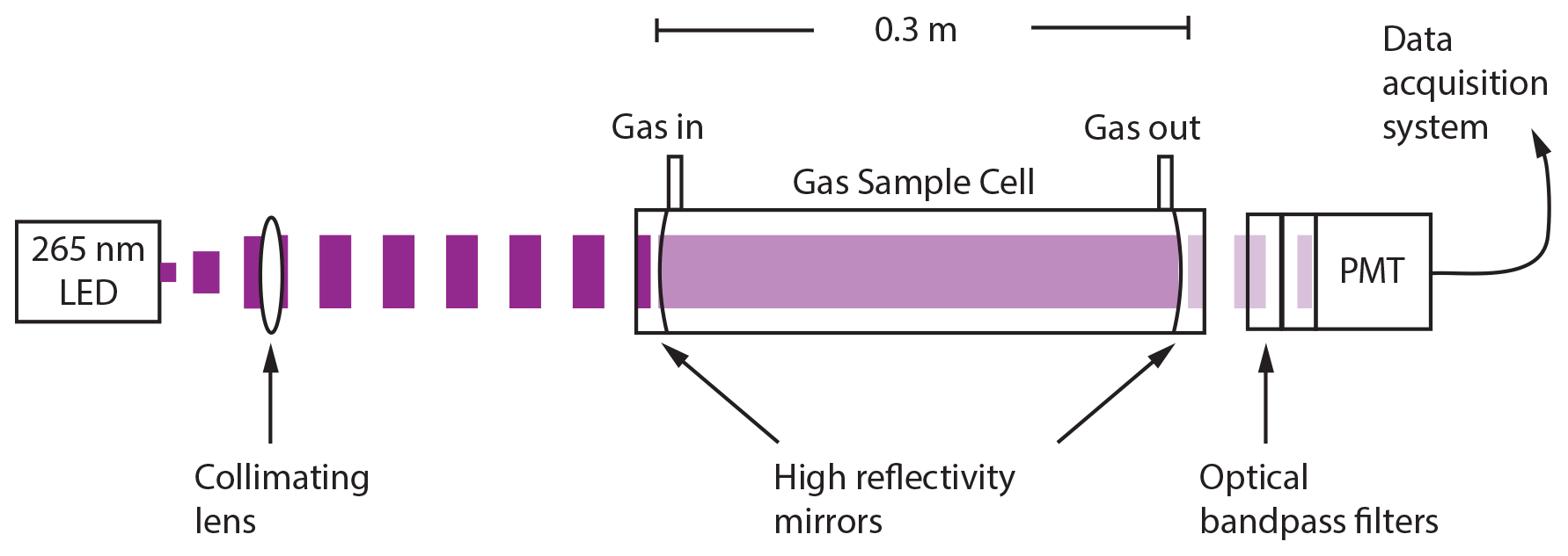
Figure 1 Incoherent broadband cavity-enhanced detection technique for O₃. An LED at 265 nm is collimated with a lens and coupled into the detection cell via high-reflectivity mirrors (R>99.7 %) that comprise the optical cavity and create a long effective optical pathlength. The light attenuated by the sample is then detected using a photomultiplier tube (PMT) operated in analog mode. The sample enters and exits the cell orthogonal to the beam propagation.

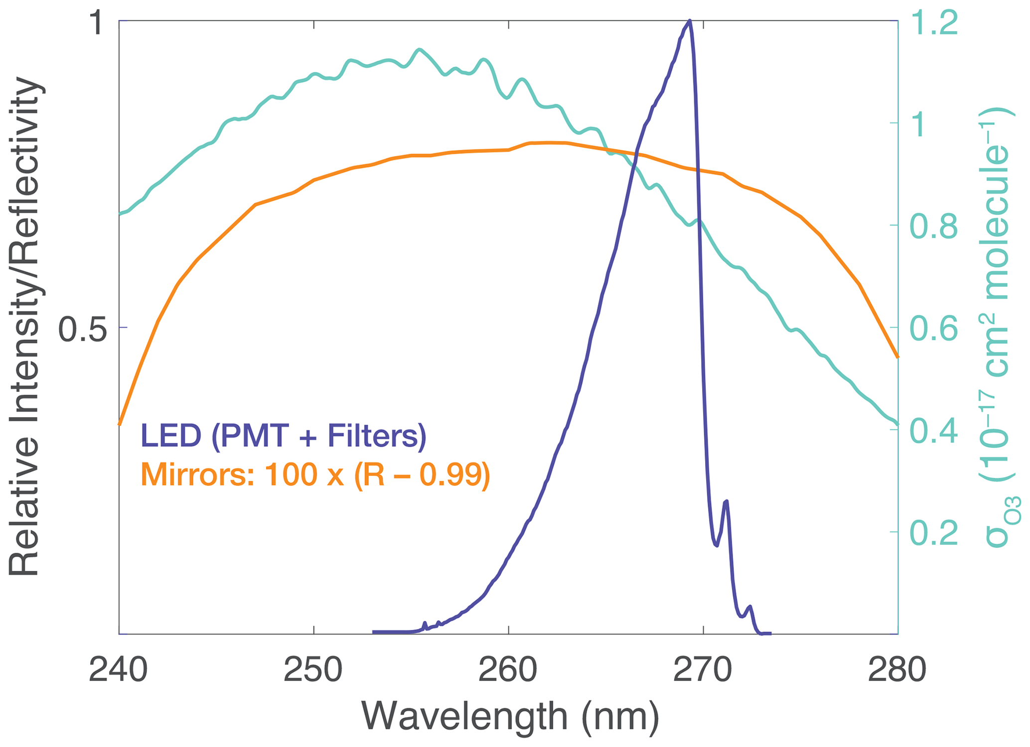
Figure 2 LED spectrum, mirror reflectivity, and O₃ absorption cross section: the LED (λ_max=265 nm, FWHM = 10 nm; full width at half maximum) spectrum was measured using a grating spectrometer (0.1 nm resolution) with the instrument PMT and associated detector optics. The mirror curve depicts $\mathrm{100}\times \left[R-\mathrm{0.99}\right]$, where R is the reflectivity, over a range of wavelengths. The right axis shows the absorption cross section for the O₃ Hartley band. O₃ and Rayleigh cross sections were determined as the weighted average with the normalized intensity of the LED and PMT detector optics.

Attenuation of light intensity in an IBBCEAS cavity results from trace gas absorption as well as extinction due to the mirrors and Rayleigh scatter. Accounting for these additional losses, the Beer–Lambert absorption coefficient, α_abs, is related to the observed change in intensity transmitted through the cavity as follows (Washenfelder et al., 2008):

$$\begin{array}{}\text{(1)}& {\mathit{\alpha }}_{\mathrm{abs}}=\left({\displaystyle \frac{I_{\mathrm{0}}-I}{I}}\right)\left({\displaystyle \frac{\mathrm{1}-R}{d}}+{\mathit{\alpha }}_{\mathrm{Ray}}\right).\end{array}$$

Here, I₀ is light intensity in the absence of any absorbing species; I is the intensity attenuated due to absorption; R is the mirror reflectivity; d is the physical distance separating the cavity mirrors; and α_Ray is the extinction due to Rayleigh scatter, a non-negligible component in the UV. The term $(\mathrm{1}-R)/d$ gives the theoretical cavity loss, α_cav, and represents the inverse of the maximum effective optical pathlength, L_eff. In cavity-enhanced techniques, L_eff can be many orders of magnitude larger than d, resulting in high sensitivity to the absorbing species. Equation (1) can also be expressed as α_abs=Nσ_abs, where N is number density of the absorbing species and σ_abs is the absorption cross section. In principle, accurate trace gas measurements require calibration of the α_cav term yielding L_eff, knowledge of the Rayleigh and absorption cross sections in the detected spectral region, and the measured I₀ and I terms. The data processing and calibration for ROZE will be discussed in Sects. 3.4 and 4.1, respectively.

3 Instrument description

ROZE consists of three main subsystems housed in a compact 58 cm long × 44 cm wide × 18 cm high chassis, with a total instrument weight of 19 kg (Fig. 3). The optical plate – a custom aluminum honeycomb panel supported by friction-dampened spring vibration isolators – provides a stable platform for the optical components, consisting of the LED, sample cell, and PMT. The remaining subsystems include the flow handling and the data acquisition. Each major subsystem is described in greater detail below. ROZE operates at 24 V_DC with a low-profile AC-DC switching power supply (Vicor VI-LU3-IU) capable of running off 115 or 230 V_AC (47–440 Hz), which can be supplied directly from the aircraft. Power consumption is less than 200 W and typically ∼ 100 W. Table 1 summarizes ROZE design and performance characteristics.

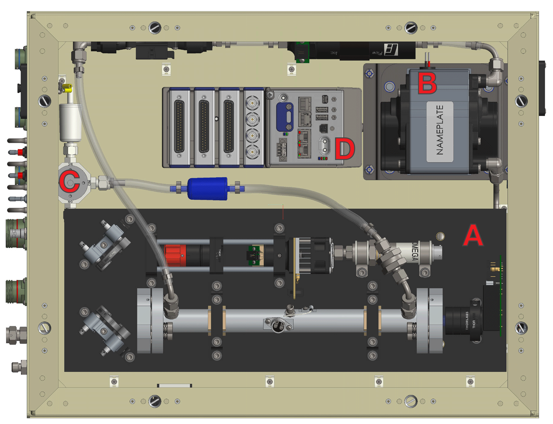
Figure 3 A top view of the ROZE instrument chassis. Major components include (a) the optical plate, which consists of the LED assembly, associated optics, the optical cell, and the PMT detector; (b) the diaphragm pump which can pull up to ∼ 18 SLM (standard liter per minute) through the flow system; (c) the three-way valve which switches between the sample line and air scrubbed of O₃ using a Carulite filter; and (d) the data acquisition system.

Table 1 Summary of ROZE performance capabilities.

3.1 Optical components

3.1.1 LED assembly

A UV LED (λ_max=265 nm, FWHM = 10 nm) (Thorlabs M265D2) is mounted to a custom heat sink and temperature-controlled to 30 ^∘C with a thermoelectric cooler (TE Technology CH-21-1.0-1.3 and Wavelength Electronics PTC2.5K-CH). The LED output power is separately monitored by a photodiode (Marktech MTPD4400D-1.5) inserted into the edge of a lens tube that holds the LED. The LED assembly attaches to a custom cage mount system that also houses the associated optics, including the aspheric collimation lens (f=79 mm, Thorlabs ASL10142M) and a beam expander (Thorlabs BE02-UVB) in reverse to shrink the collimated LED output. For compactness, the LED assembly and cage system are mounted parallel to the sample cell, and two mirrors (Thorlabs NB1-K04) turn the beam 180^∘ into the cell (see Fig. 3).

3.1.2 Sample cell

The sample cell is manufactured from an aluminum alloy tube measuring 30 cm in length with a 1.2 cm inner diameter. The cell mirrors (Layertec 109561) have a reflectivity of R>99.7 % over the detected spectral range (Fig. 2) and a 500 mm radius of curvature. The mirrors are held directly at the cell ends on face type o-ring seals using custom, non-adjustable mounts fastened to tube collars. The mirror positions are configured to maximize centricity. Two gas ports direct the sample flow into and out of the cell at right angles. The sample enters through a custom stainless-steel cylindrical diffuser, a ring with circumferential openings adjacent to the cell mirrors, that nests within the cell tube orthogonal to the ports. The diffuser helps minimize noise due to Rayleigh scatter from turbulence within the cell at high sample flow rates. A 2 µm pleated mesh filter (Swagelock) affixes to the sample cell inlet port to exclude dust and other particles from affecting the mirror reflectivity, as the mirrors are not independently purged. A pressure transducer (Omega MMA015V10P4K1T4A6) measures the cell pressure from a port near the cell center. The entire cell is thermally regulated to 35 ^∘C using resistive heaters and a precision heater control (Wavelength Electronic PTC2.5K-CH).

3.1.3 PMT assembly

A PMT (Hamamatsu H10720-113) operating in analog mode collects the light exiting the cell. Two optical bandpass filters (Thorlabs FGUV5-UV and Semrock FF01-260/16) transmit the cell output to a collection lens (f=35 mm, Thorlabs LA4052-UV), which images the beam onto the PMT photocathode. A UV window (Thorlabs WG40530-UV) glued into a custom PEEK lens tube adapter seals to the PMT face with a Viton gasket, creating a leak-tight package for low-pressure (high-altitude) operation. The PMT is thermally stabilized to 35 ^∘C in the same manner as the sample cell. The PMT signal is passed to an amplifier circuit (Analog Devices EVAL-ADA4625-1ARDZ) before digitization by the data acquisition system described below.

3.2 Flow system

The ROZE flow system is designed to achieve rapid flushing of the detection cell as required for fast concentration measurements. However, ROZE samples at ambient pressure to maximize sensitivity, necessitating high throughput with a minimal pressure differential. ROZE utilizes a linear diaphragm pump (Thomas 6025SE-150113) that can achieve a flow rate of up to 18 SLM (standard liter per minute) through the system. The pump speed can also be adjusted by varying the supply current and has three pre-set speeds (e.g., 2, 5, and 11 SLM) that can be changed by a switch on the chassis front panel. A flow meter (Honeywell AWM5104) located between the cell exhaust and the pump monitors the sample flow in real time. ROZE uses fluorinated ethylene propylene (FEP) tubing both external and internal to the chassis upstream of the sample cell. External to the chassis, the inlet details depend on the aircraft platform. ROZE has previously used the inlet detailed in Cazorla et al. (2015) when flying on the NASA DC-8 aircraft. The instrument exhaust plumbs directly to an exhaust port near the rear of the aircraft.

ROZE O₃ measurements also require knowledge of the reference intensity (I₀) as detailed in Eq. (1). A three-way solenoid valve (NResearch TC648T032) switches between the sample line (ambient air from the aircraft inlet) and the zero port, which attaches to an internal Carulite O₃ scrubber (2B Technologies) to produce O₃-free air. Periodic zeroing during operation captures long-term drift in I₀ due to the LED output, PMT response, and changing environmental conditions. Typically, the instrument opens to the O₃ scrubber for 10 s every 5 min.

3.3 Data acquisition

ROZE utilizes a CompactRIO (National Instruments cRIO-9030) that incorporates a real-time operating system and a field-programmable gate array (FPGA). The FPGA is configured for modulation of the LED and subsequent digitization of the PMT signal. To improve measurement precision and remove background due to ambient light scatter, the FPGA modulates the LED at 1 kHz with a 90 % duty cycle (900 µs on and 100 µs off) via an external LED driver (Wavelength Electronics FL591FL). A 16 bit analog-to-digital converter (ADC) digitizes the amplified PMT signal at a digitization rate of 100 kHz. This high rate enables us to average each LED “on” and “off” pulse amplitude. We then take the difference of the on and off signals to remove background noise, both optical (i.e., stray light) and electronic. The 1 kHz differences are further averaged to 10 Hz and recorded. Other diagnostic housekeeping variables (e.g., sample flow, temperatures, and LED power) are recorded at 1 Hz. Additionally, an analog output commands the three-way valve to open to the zero line with a user-defined period and duration.

3.4 Data processing

In practice, the absorbance calculation for ROZE factors in the pressure difference between the sample and zero lines, as derived by Min et al. (2016):

$$\begin{array}{}\text{(2)}& {\mathit{\alpha }}_{{\mathrm{O}}_{\mathrm{3}}}=\left({\displaystyle \frac{I_{\mathrm{Z}}}{I}}-\mathrm{1}\right)\left({\mathit{\alpha }}_{\mathrm{cav}}+{\mathit{\alpha }}_{\mathrm{Ray},\mathrm{Z}}\right)+\mathrm{\Delta }{\mathit{\alpha }}_{\mathrm{Ray}}.\end{array}$$

Analogous to Eq. (1), I_Z is the intensity measured when sampling through the zero line (O₃-scrubbed air); I is the intensity when sampling ambient air; and $\mathrm{\Delta }{\mathit{\alpha }}_{\mathrm{Ray}}={\mathit{\alpha }}_{\mathrm{Ray},\mathrm{Z}}-{\mathit{\alpha }}_{\mathrm{Ray},\mathrm{S}}$, where α_Ray,Z and α_Ray,S give the Rayleigh extinction (α_Ray=N_airσ_Ray) of the zero and the sample, respectively. Using the measured I_Z, I, and the known Rayleigh scatter and O₃ absorption cross sections, the O₃ number density can then be determined as ${\mathit{\alpha }}_{{\mathrm{O}}_{\mathrm{3}}}=N_{{\mathrm{O}}_{\mathrm{3}}}{\mathit{\sigma }}_{{\mathrm{O}}_{\mathrm{3}}}$. The Rayleigh scattering (Bucholtz, 1995) and O₃ absorption (Serdyuchenko et al., 2014) cross sections are calculated as the weighted average over the collected spectral range (Fig. 2). Using known cross sections and a calibrated α_cav (inverse effective pathlength), the observed change in intensity yields a direct measure of the O₃ concentration.

4 Performance

4.1 Sensitivity and calibration

The effective pathlength of the ROZE optical cavity determines the instrument sensitivity to O₃ (i.e., the attenuation in intensity per unit O₃). The cavity extinction, and thus the effective pathlength, are dictated by the mirror reflectivity as described above but require independent calibration. Calibration can be accomplished via standard addition of O₃ or Rayleigh attenuation (in the absence of absorbing species) at varied sample pressures. The former method relies on commercially available O₃ generators or sensors for verification, which lack the required accuracy and may drift over time. In contrast, the Rayleigh calibration provides a convenient and straightforward alternative. Both methods are described below.

Figure 4a depicts the ROZE calibration using known concentrations of O₃. A commercial O₃ source (2B Technologies 306) generated known amounts of O₃, with the zero O₃ addition serving as the I_Z baseline. Per Eq. (2), the slope of the observed attenuation (d$I=I_{\mathrm{Z}}/I-\mathrm{1})$ as a function of O₃ number density is proportional to the remaining extinction terms (α_cav+α_Ray). Solving for α_cav using the O₃ cross section and the calculated Rayleigh extinction, the calibration yields an effective pathlength of L_eff=108 ± 6 m. The alternate calibration uses the Rayleigh extinction in zero air over a range of cell pressures (Fig. 4b). In the absence of absorbing species, an expression for α_cav can be derived following the approach in Washenfelder et al. (2008) as

$$\begin{array}{}\text{(3)}& {\mathit{\alpha }}_{\mathrm{Ray}}=\left({\displaystyle \frac{I_{\mathrm{0}}}{I}}-\mathrm{1}\right){\mathit{\alpha }}_{\mathrm{cav}}.\end{array}$$

I₀ represents the intensity at vacuum, which can be extrapolated from a linear fit of counts as a function of cell pressure. The slope of the observed change in intensity with number density therefore yields a direct measure of the cavity extinction, resulting in an effective pathlength of 104 ± 4 m. The two methods agree to within the 2σ fit uncertainties, and we use L_eff as determined by the Rayleigh calibration for subsequent calculations.

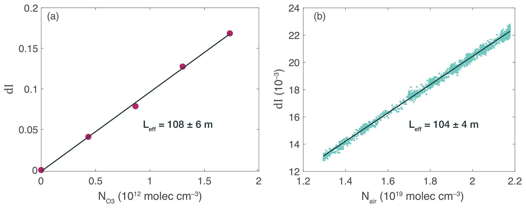
Figure 4 ROZE calibration. (a) The effective pathlength (L_eff) as determined by attenuation (dl) due to known additions of O₃ from a commercial ozone generator. The slope yields the effective pathlength as determined from Eq. (1) in the text using the known O₃ absorption cross section. (b) Attenuation due to Rayleigh scatter over a range of cell pressures. The slope of attenuation as a function of number density gives the pathlength using the known Rayleigh scattering cross section for zero air. The pathlength derived from both calibrations agree to within the 2σ fit uncertainty.

4.2 Precision and accuracy

The major contributions to instrument noise include PMT electrical noise and differential scatter or absorption due to non-uniform flow within the sample cell at high flow rates. The flow diffuser (see Sect. 3.1.2) effectively reduces the flow noise, while decreasing the gain on the PMT amplifier circuit minimizes the PMT electrical noise. The ROZE precision can be determined from the continuous sampling of zero air at a constant pressure. Figure 5 depicts the Allan–Werle deviation plot (1σ) for ROZE (in pptv – parts per trillion by volume – O₃ equivalents) as calculated from optical extinction measurements of zero air acquired over 1.5 h at 944 mbar. For short integration times (<10 s), a fit of the data gives a τ^−0.47 decay, indicating the Allan deviation closely follows the square root of the averaging time (${\mathit{\tau }}^{-\mathrm{1}/\mathrm{2}}$) as expected for white noise. At the native 0.1 s sampling rate, the 1σ precision for O₃ is 80 pptv and reduces to 31 pptv with 1 s averaging. For the given cell pressure and a temperature of 35 ^∘C, this translates to a 1σ precision of 6.7×10⁸ molecules cm⁻³ (1 s average) of O₃.

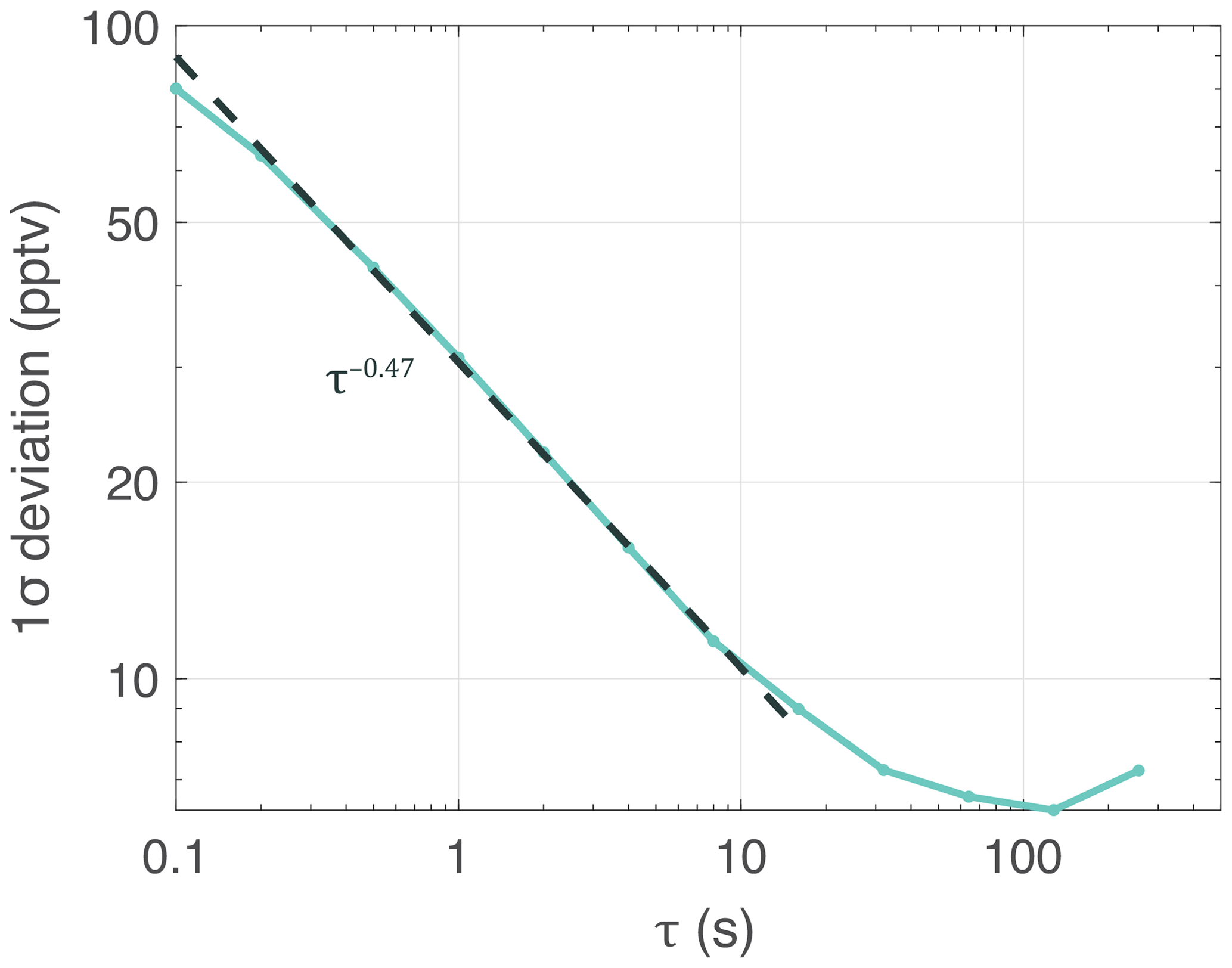
Figure 5 Allan deviation plot for 1.5 h of sampling zero air at constant pressure (944 mbar). The 1σ precision is expressed in pptv equivalents of O₃ as a function of the integration time τ. The curve demonstrates a precision of 31 pptv in a 1 s integration time. The dashed line shows a τ^−0.47 decay for short integration times (<10 s), comparable to the ${\mathit{\tau }}^{-\mathrm{1}/\mathrm{2}}$ decay expected for white noise.

The absolute accuracy of the ROZE measurement depends on uncertainties in the literature-reported values of the O₃ and Rayleigh cross sections, the measured cell temperature and pressure, and the calibrated cavity extinction. The reported O₃ absorption cross section has an uncertainty of 2 % (Gorshelev et al., 2014), and we estimate a conservative uncertainty of 3 % for the Rayleigh scattering cross section (Bucholtz, 1995). The cell pressure and temperature are accurate to within 0.2 % and 0.5 %, respectively, and the calibrated cavity extinction has an additional 4 % slope uncertainty from the linear fit. These errors propagate through Eq. (2) to yield a total measurement uncertainty of 6.2 % in the O₃ number density.

4.3 Response time

The flush time of the sample cell limits the true instrument response time despite the 10 Hz data acquisition rate. A rapid flush rate is critical for high-spatial-resolution measurements from a fast-moving platform. Additionally, fast concentration measurements are required for sampling turbulent eddies for airborne EC, and the necessary time response scales with aircraft speed. Response times of 10 Hz are typically considered sufficient for ground-based EC (Aubinet et al., 2012), while for airborne EC, a response time of 1–5 Hz is typically sufficient due to larger eddy scales at altitude (Wolfe et al., 2018). Figure 6a shows the instantaneous instrument response to a 10 ms pulse of O₃ injected into a zero-air carrier flow using a fast switching valve (The Lee Company IEP series). During this experiment, the pump maintained a sample flow rate of 18 SLM. A series of exponential decay fits for several O₃ pulses yields an e-folding time constant of ${\mathit{\tau }}_{\mathrm{r}}=\mathrm{50}\pm \mathrm{4}$ ms (Fig. 6b), which corresponds to a 3e-fold cell flush rate of 9.5 Hz.

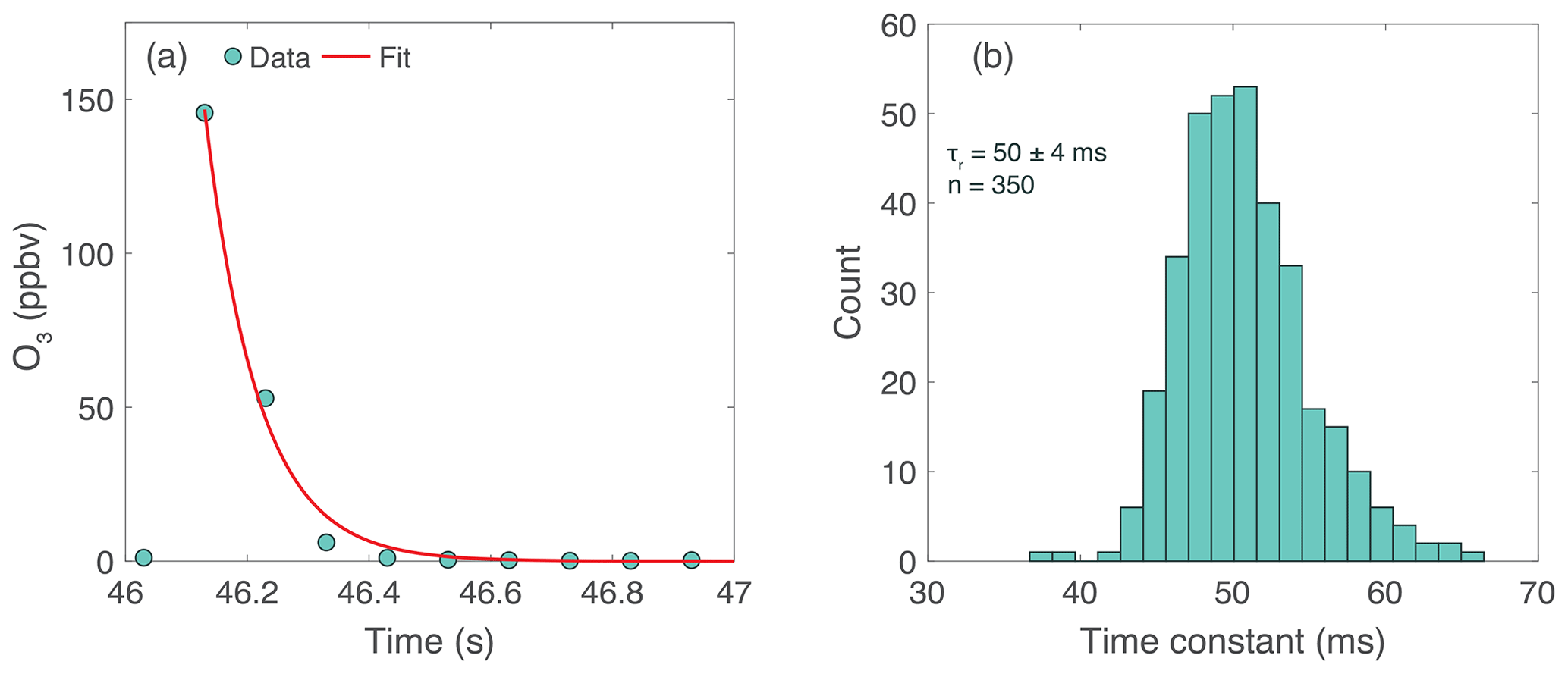
Figure 6 ROZE time response. (a) Ozone was injected into the flow system via a pulsed valve at 2 s intervals with a sample flow of 18 SLM. An exponential decay function was fitted to each individual pulse (pulse data shown in blue; fit shown in red). (b) Histogram of time constants for all 350 pulses. The e-folding decay time of 50 ± 4 ms corresponds to a 3e-fold cell flush rate of 9.5 Hz.

5 Field demonstration

ROZE can be operated on both low- and high-altitude aircraft platforms. Though ROZE has not yet flown on a high-altitude unpressurized aircraft (such as the NASA ER-2), laboratory experiments in a thermal-vacuum chamber have demonstrated no loss of performance down to a pressure and temperature of 50 mbar and 250 K (results not shown). In summer 2019, ROZE flew aboard the NASA DC-8 for the Fire Influence on Regional to Global Environments Experiment, Air Quality (FIREX-AQ) campaign over the central and northwestern United States. The instrument operated as described above, with the addition of an inline particle filter (Balston 9922-05-DQ) to protect the cavity mirrors from fine particulates in the targeted smoke plumes. Although more aggressive filtering comes at the cost of reduced flow rates and thus lowers the instrument response time, O₃ deposition measurements were not a primary objective of FIREX-AQ. Below, we detail comparisons of ROZE against an established O₃ measurement. Additionally, level flight legs in the marine boundary layer during a flight over the ocean provide an initial demonstration of O₃ vertical-flux measurements.

5.1 FIREX-AQ validation against chemiluminescence

FIREX-AQ flights targeted forest wildfires and agricultural burns. In fresh, concentrated smoke plumes, UV-active species such as SO₂, aromatic hydrocarbons, and other volatile organic compounds (VOCs) can give rise to positive artifacts in the O₃ signal (Long et al., 2020), as the UV absorption technique lacks selectivity (see Birks, 2015). The potential for overestimating O₃ due to interfering absorbers can also be of concern in highly polluted urban environments (e.g., Spicer et al., 2010). In general, these studies demonstrate that UV-absorption-based O₃ analyzers are not always ideally suited to such applications. Nonetheless, modifications such using an O₃-selective scrubber material (e.g., heated graphite) to preserve VOCs and thus account for interferences in the background (I_Z) signal have been shown to reduce positive artifacts (Turnipseed et al., 2017). As we did not substitute the ROZE scrubber for the FIREX-AQ deployment, an onboard, independent measurement of formaldehyde (HCHO) was used as a plume indicator. ROZE O₃ data are therefore quality-filtered to remove points sampled within dense smoke plumes using HCHO mixing ratios above 5 ppbv.

The DC-8 FIREX-AQ payload included the NOAA Nitrogen Oxides and Ozone (NOyO3) instrument, a well-established O₃ measurement using the chemiluminescence technique (Ryerson et al., 2000; Bourgeois et al., 2020). ROZE operated simultaneously with the NOyO3 instrument during several flights. Figure 7 shows a comparison of ROZE and NOyO3 data for the 30 July 2019 flight over the northwestern United States. During this flight, no fresh smoke plumes were sampled, and no filtering of the ROZE data was necessary. Figure 7a depicts a ∼ 25 min subset of the full time series to illustrate the ROZE instrument precision. Both measurements (averaged to 1 s) track the dynamic features in O₃ mixing ratios well. The correlation plot for the full flight (Fig. 7b) demonstrates strong agreement between the two measurements, with a slope of 0.98 ± 0.01 and an intercept of 0.17 ± 0.02 ppbv O₃ (r²=0.99). Note the intercept is less than 1 % of the minimum observed O₃ mixing ratios for this flight. Comparisons for 15 flights from the campaign indicate a range of 0.96–1.04 in slope and −1.6–1.4 ppbv O₃ in intercept (in all cases, this offset is <4 % of the minimum measured O₃), consistent with the measurement uncertainty.

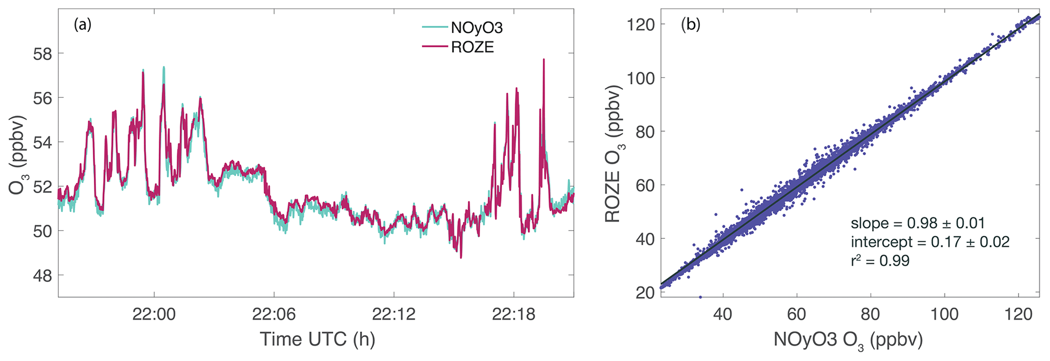
Figure 7 ROZE and NOyO3 measurements of O₃ from a FIREX-AQ flight on 30 July 2019 over the northwestern US. (a) Time series of ROZE and NOyO3 data (averaged to 1 s). (b) Correlation plot of ROZE and NOyO3 O₃ measurements from the full flight. A linear fit to the data yields a slope of 0.98 ± 0.01 and an intercept of 0.17 ± 0.02 ppbv.

5.2 Ozone flux measurements

5.2.1 Eddy covariance flux

The vertical flux of O₃ can be directly quantified using the eddy covariance (EC) technique. EC defines the flux (F) as the temporally or spatially averaged covariances in the vertical wind speed (w) and the scalar species of interest (in this case the O₃ mixing ratio $X_{{\mathrm{O}}_{\mathrm{3}}}$):

$$\begin{array}{}\text{(4)}& F_{{\mathrm{O}}_{\mathrm{3}}}=\langle w^{\prime }{X}_{{\mathrm{O}}_{\mathrm{3}}}^{\prime }\rangle .\end{array}$$

In the equation above, the primes denote instantaneous deviations from the mean value, and the brackets indicate an average over a prescribed interval as discussed below. Since deposition dominates transfer across the air–surface interface, the O₃ flux can instead be expressed as a transfer rate or deposition velocity (v_d):

$$\begin{array}{}\text{(5)}& v_{\mathrm{d}}=-{\displaystyle \frac{F_{{\mathrm{O}}_{\mathrm{3}}}}{{\overline{X}}_{{\mathrm{O}}_{\mathrm{3}}}}}.\end{array}$$

Here, the overbar indicates the mean O₃ mixing ratio over the averaging period. The deposition velocity, in units of cm s⁻¹, yields a normalized metric of the deposition efficiency and incorporates both chemical and physical transfer processes.

During the FIREX-AQ campaign, the flight on 17 July 2019 contained a level segment within the turbulent marine boundary layer suitable for EC. The flux transects were located over the Pacific Ocean, ∼ 200 miles southwest of the Los Angeles basin. To quantify O₃ deposition, the Meteorological Measurement System (MMS) instrument provided 3-D wind vector data (Chan et al., 1998), which were used in conjunction with ROZE O₃ measurements. A 1-D coordinate rotation was applied to the wind vector to force the mean vertical wind to zero, and the native 20 Hz MMS data were averaged to the ROZE 10 Hz time base. Note that the additional particle filter reduced the ROZE sample flow to 11.3 SLM, and we estimate the time constant from the decay in intensity following the zero-O₃ additions as τ_r=90 ms (5.5 Hz 3e-fold flush rate). We also use 20 Hz water vapor measurements from the open-path Diode Laser Hygrometer (DLH) (Diskin et al., 2002) as a benchmark for the flux performance; 20 Hz DLH data were averaged to the ROZE time base and used to apply a moist-to-dry air correction for raw O₃ observations, negating the need for density corrections to the calculated flux (Webb et al., 1980). This density correction reduces the O₃ flux by ∼ 6 %. For the EC calculations, we selected two ∼ 50 km transects with consistent aircraft heading, stationary flow, and level altitude (∼ 170 m). Scalar data were detrended by subtracting a 20 s running mean, which corresponds to spatial scales of ∼ 2.7 km. The detrending length was chosen to remove non-turbulent variability (e.g., changing chemical conditions) while still capturing the largest flux-contributing eddies as identified by examination of the co-spectra from a range of averaging windows. Scalar data were then synchronized to the vertical winds using a time lag that optimized covariance.

5.2.2 Spectral analysis

Spectral analysis aids in decomposing the contributions of eddies at different scales (frequencies) to the overall signal and provides a quality assessment of the ROZE flux measurements. Figure 8 displays the lag covariance, power spectrum, and co-spectrum for O₃ and vertical-wind fluctuations generated using fast Fourier transforms (FFTs) for a single transect. The spectra for water vapor are also displayed for comparison. The lagged cross-cross-covariance functions (Fig. 8a) demonstrate defined peaks at lags of <0.5 s, with the peak non-normalized covariance yielding a measure of the flux. Dividing out the background O₃ mixing ratio of 29 ppbv, we find a mean deposition velocity of 0.029 cm s⁻¹ for the two transects. The power spectra in Fig. 8b show that vertical winds follow the theoretical $f^{-\mathrm{5}/\mathrm{3}}$ decay expected in the inertial subrange (Kaimal et al., 1972). The slope for the O₃ power spectrum initially follows the same decay but flattens at ∼ 1 Hz, indicating that the turbulence-driven variability in O₃ approaches the ROZE precision limit in higher-frequency eddies. However, the normalized frequency-weighted co-spectral power of w^′ with $X_{{\mathrm{O}}_{\mathrm{3}}}^{\prime }$ (Fig. 8c, solid lines) shows that flux-carrying eddies below ∼ 0.6 Hz dominate the total signal. The ogive, the cumulative integral of the co-spectrum (Fig. 8c, dashed lines) further indicates that 99 % of flux-carrying eddies occur at frequencies below ∼ 4 Hz. These results demonstrate the adequate ROZE time response for airborne EC.

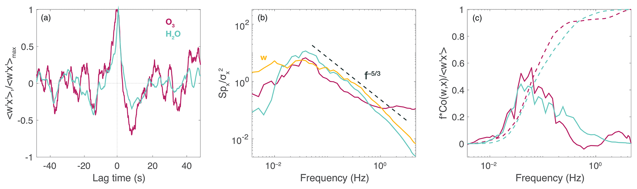
Figure 8 Example spectra from a 50 km flux leg at 170 m altitude during the 17 July 2019 flight over the Pacific Ocean. (a) Vertical-wind-scalar (w and x, respectively) cross-covariance functions normalized by the maximum covariance for O₃ and water vapor. (b) Power spectra normalized to total variance for w, O₃, and H₂O. The dashed line represents the $f^{-\mathrm{5}/\mathrm{3}}$ theoretical decay for the inertial subrange. (c) Solid lines depict co-spectral power (frequency-multiplied and covariance-normalized) of O₃ and H₂O with vertical wind. Dashed lines depict the respective ogives (cumulative integrals).

5.2.3 Flux measurement uncertainty

Detailed methods to quantify flux errors for airborne EC can be found elsewhere (Lenschow et al., 1994; Langford et al., 2015; Wolfe et al., 2018). Here, we aim to quantify the random and systematic flux errors that reflect the overall instrument performance. We use the empirical formulation of Finkelstein and Sims (2001) to estimate the total random error (RE_TOT) as the variance of the scalar-wind covariance. In this approach, the RE_TOT is determined using auto- and cross-correlation functions (as in Fig. 8a) over lag times that are sufficient to capture the timescale of the correlation (here ∼ 10 s). Averaging over the flux legs yields a RE_TOT of 0.005 cm s⁻¹. The RE_TOT encompasses both instrument noise as well as error from the random sampling of turbulence. To isolate the RE component due solely to instrument noise (RE_noise), we follow the approach of Mauder et al. (2013). In this method, the standard deviation of the instrument noise is derived from the scalar auto-covariance and then propagated to determine its contribution to the cross-covariance uncertainty. Note that RE_noise still depends on the turbulence regime and therefore varies with atmospheric conditions. We calculate RE_noise to be 0.0015 cm s⁻¹ averaging over the two flux transects. These results indicate that instrument noise constitutes ∼ 30 % of the total random error.

Additionally, the instrument time response can lead to systematic flux errors as a consequence of undersampling contributions from high-frequency eddies. We determine the systematic error due to the instrument response time (SE_RT) following the Horst (1997) model, whereby the attenuation in the measured signal can be expressed as a co-spectral transfer function based on the characteristic instrument response time. Using the ROZE response time of τ_r=90 ms, we determine SE_RT to be <2 %, indicating minimal attenuation in the measured flux signal.

6 Summary and conclusions

The NASA ROZE instrument provides high-sensitivity, fast-time-response measurements of O₃ via broadband cavity-enhanced UV absorption. The compact, robust instrument package is adaptable to diverse field environments, including low- and high-altitude aircraft platforms. ROZE currently achieves a 1σ precision of ∼ 30 pptv s⁻¹ and an overall accuracy of 6.2 %. ROZE was successfully integrated aboard the NASA DC-8 aircraft, and the field performance compares favorably with an independent O₃ measurement to within ROZE uncertainty. The maximum observed time response for laboratory tests was 50 ms, with additional filtering during aircraft operation slowing the time response to 90 ms. The instrument precision and time response make ROZE particularly well suited for measurements of vertical O₃ flux using eddy covariance analysis. ROZE has measured O₃ deposition velocities of 0.029 ± 0.005 cm s⁻¹ to the ocean surface, with minimal (<2 %) response time attenuation in the flux signal. The demonstrated performance of ROZE makes the instrument an ideal and versatile option for field measurements of both O₃ concentrations and fluxes.