Integrated System for Atmospheric Boundary Layer Height Estimation (ISABLE) using a ceilometer and microwave radiometer

Accurate boundary layer structure and height are critical in the analysis of the features of air pollutants and local circulation. Although surface-based remote sensing instruments provide a high temporal resolution of the boundary layer structure, there are numerous uncertainties in terms of the accurate determination of the atmospheric boundary layer heights (ABLHs). In this study, an algorithm for an integrated system for ABLH estimation (ISABLE) was developed and applied to the vertical profile data obtained using a ceilometer and a microwave radiometer in Seoul city, Korea. A maximum of 19 ABLHs were estimated via the conventional time-variance, gradient, wavelet, and clustering methods using the backscatter coefficient from the ceilometer. Meanwhile, several stable boundary layer heights were extracted through near-surface inversion and environmental lapse rate methods using the potential temperature from the microwave radiometer. The ISABLE algorithm can find an optimal ABLH from post-processing, such as k-means clustering and density-based spatial clustering of applications with noise (DBSCAN) techniques. It was found that the ABLH determined using ISABLE exhibited more significant correlation coefficients and smaller mean bias and root mean square error between the radiosonde-derived ABLHs than those obtained using the most conventional methods. Clear skies exhibited higher daytime ABLH than cloudy skies, and the daily maximum ABLH was recorded in summer because of the more intense radiation. The ABLHs estimated by ISABLE are expected to contribute to the parameterization of vertical diffusion in the atmospheric boundary layer.

1 Introduction

The atmospheric boundary layer (ABL) is the lowest part of the troposphere, which is directly influenced by the surface of the earth (Garratt, 1994). The ABL is repeated in a daily cycle with a well-mixed layer (ML) or a convective boundary layer (CBL) in the daytime and a stable boundary layer (SBL) at nighttime. The former mixes air vertically via convection which results from surface heating or mechanical turbulence due to vertical wind shear, while the latter appears in the lower ABL, and a residual layer (RL) remains in the upper ABL without any external force. The ML is one of the essential meteorological factors that affect the vertical mixing of air pollutants. In the presence of a well-developed SBL at night, air pollutants near the surface tend to be trapped inside the SBL because of the low vertical diffusivity, and their concentrations could increase sharply (Stull, 1988; Emeis and Schäfer, 2006). In this study, the ABL is confined as a single layer, which is consisted of a ML or a SBL to exclude its complexity.

The ABL height (ABLH) has been primarily utilized as a meteorological factor in estimating the vertical diffusivity near the surface and air pollutant concentration (Stull, 1988; Garratt, 1993). Many previous studies have developed various methodologies for determining ABLH, including only a ML height (MLH) or a SBL height (SBLH). ABLH has traditionally been determined using in situ radiosonde (RS) data. The parcel method using the vertical profile of virtual potential temperature (Holzworth, 1964; Seibert et al., 2000) and the gradient method using the vertical gradient of the virtual potential temperature or mixing ratio have been extensively used (Oke, 1987; Stull, 1988). Alternatively, ABLH can be determined using the bulk Richardson number, which includes the thermal turbulence term generated by surface heating as well as the mechanical turbulence term arising from the vertical wind shear (Vogelezang and Holtslag, 1996; Zilitinkevich and Baklanov, 2002; Zhang et al., 2014). The ABLH estimated using in situ RS sounding has widely been considered as a true reference value in many previous studies (e.g., Eresmaa et al., 2006; Basha and Ratnam, 2009; and Collaud Coen et al., 2014). However, there are still some limitations in terms of clearly distinguishing ABLH from radiosonde observations (Seibert et al., 2000). ABLH tends to be determined as similar values irrespective of the methodologies used under a well-developed convective boundary layer (BL) during daytime and SBL at night, while it gives different values with respect to methodologies under a cloudy sky and in the presence of complex local circulations. Furthermore, the major drawback of RS sounding data their its coarse temporal resolution ranging from 6 to 12 h (Schween et al., 2014).

During the past two decades, several researchers have determined ABLH using surface-based remote sensing instruments to overcome the coarse resolution of RS data. An aerosol lidar and a lidar-type ceilometer (hereinafter referred to as merely ceilometer) measure the intensity of signals which have been backscattered by atmospheric materials, such as aerosols, clouds, and mineral dust. The intensity of the backscattered signal at each level can be converted to the backscattering coefficient at the level with several assumptions. The measured backscattering coefficient can be used to analyze the features of the vertical distribution of aerosols, while the ABLH can be determined through the separation of aerosol layers. In a ML, the vertical mixing of aerosol particles is active and the backscattering coefficient is relatively homogeneous, whereas it decreases sharply above the MLH. Based on the foregoing features, the gradient method designates the altitude with the maximum vertical gradient of the backscattering coefficient as the ABLH (e.g., Flamant et al., 1997; Sicard et al., 2005; Lammert and Bösenberg, 2006; Münkel et al., 2007; Emeis et al., 2008; Summa et al., 2013; and Schween et al., 2014). The wavelet method determines ABLH as the altitude at which the wavelet covariance coefficient is at its maximum (e.g., Gamage and Hageberg, 1993; Cohn and Angevine, 2000; Brooks, 2003; and Morille et al., 2007). Menut et al. (1999) analyzed the ABL structure using the inflection point method (second derivative method) and centroid method (time-variance method) for the purpose of understanding the chemical and physical processes involved in pollution events in Paris. The growth and decline of the ABLH are repetitive due to the heating and cooling of the surface. As a result, the vertical aerosol distribution in the aerosol layer changes with time, and the ABLH can therefore be determined using the time variance of the aerosol temporal distribution. Toledo et al. (2014) and Caicedo et al. (2017) determined ABLH as a classification of the distribution of the backscattering coefficient value whose vertical profile rapidly decreases or increases using k-means clustering. Moreover, the ABLH was estimated using an extended Kalman filter (EKF) (Lange et al., 2014, 2015; Saeed et al., 2016). The EKF technique can be used in low signal-to-noise ratio (SNR) atmospheric scenarios without long-time averaging and range smoothing except for low SNR (Dang et al., 2019). Previous studies integrated multiple methodologies; i.e., Pal et al. (2013) combined the gradient method based on a first derivative of the Gaussian wavelet covariance analysis and the spatial/temporal variance method; and Hicks et al. (2015) combined the error function-ideal profile method and wavelet covariance transform method to estimate ABLH.

Even though several methods have been developed, no consensus on a specific algorithm has been reached (Schween et al., 2014). Different methodologies provide different ABLHs with respect to weather conditions and phenomena. Under complicated ABL structures (e.g., presence of multiple layers of aerosols), the ABLH could be determined as different values according to the methodology used. Based on the foregoing methodologies, it is difficult to produce a single consistent ABLH with the use of ABLHs using the previous methods. Therefore, this study aims to develop an integrated system for ABLH estimation (ISABLE) to determine a single optimized ABLH with statistically significant results from several ABLH candidates. Furthermore, seasonal and diurnal variation of the ABLH in an urban area in Seoul, Korea, shall be investigated with the use of long-term ABLHs estimated using ISABLE.

Section 2 introduces the observation station and instruments used in this study. Section 3 describes the used data and pre-processing. Section 4 describes the ABLH estimation methods and ISABLE algorithm. In Sect. 5, the ABLH estimated using available methods is compared with the radiosonde-derived ABLH, and the seasonal and diurnal variation features are described. Finally, the summary and discussion on the findings are presented in Sect. 6.

2 Site and instrumentation

We used a ceilometer, a microwave radiometer (MWR), and a net radiometer installed at the Jungnang Station (127.08^∘ E, 37.59^∘ N, 45 m; Fig. 1), a supersite of UMS-Seoul (urban meteorological observation system network in the Seoul Metropolitan Area; Park et al., 2017). The station is located in Seoul city, Korea, and the surrounding buildings form an environment that can be classified as a dense urban residential area with homogeneous heights (Park, 2018). The location is classified as both urban climate zone 2 (UCZ-2; intensely developed high density) according to the urban climate zone classification (Oke, 2006) and local climate zone 2E (LCZ-2E; compact mid-rise, bare rock, or paved) according to the local climate zone classification (Stewart and Oke, 2012). Seoul city is affected by local circulation, such as sea–land and mountain–valley breezes, due to the Yellow Sea and mountainous terrain (Park and Chae, 2018).

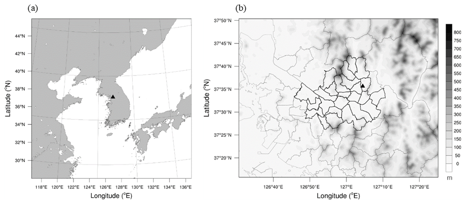
Figure 1 Location of Jungnang Station (triangle) in (a) East Asia and in (b) the Seoul Metropolitan Area with its topography.

The ceilometer (model CL51, manufacturer Vaisala) produces a real-time vertical profile of backscattering coefficients each minute at intervals of 10 up to 15 400 m above ground level using a laser (InGaAs diode laser) with a wavelength of 910 nm (Vaisala, 2010). It also measures the cloud base heights of three layers up to 13 000 m and the 5 min mean cloud cover at intervals of 1 min.

The MWR (model HATPRO-G4, manufacturer RPG) observes atmospheric attenuation and brightness temperature from electromagnetic radiation emitted from the atmosphere using 14 channels (22 to 31 GHz, 7 water vapor channels; 51 to 58 GHz, 7 temperature channels) (RPG, 2015). The measured atmospheric attenuation and brightness temperature were converted to a vertical profile of atmospheric temperature, relative humidity, and liquid water path using a neural network model. The MWR produces two types of temperature profiles, i.e., zenith measurements for the entire troposphere (0 to 10 km) and elevation scanning that provides an enhanced vertical resolution within the boundary layer (0 to 2 km). The temperature profiles of the two types are merged into a single profile. The vertical resolution is denser in the lower layer; however, it decreases with regard to height (30 m up to 1.2 km, 200 m up to 5 km, and 400 m up to 10 km), and a profile is produced every 1 min.

The net radiation obtained via the net radiometer (model CNR 4, manufacturer Kipp & Zonen) was used to classify ABLH as daytime and nighttime values (Kipp and Zonen, 2014).

3 Data and pre-processing

3.1 Radiosonde experiment

Vertical profiles observed using RS sounding are widely used in verifying surface-based remote sensing instruments because it directly observes the temperature, relative humidity (or mixing ratio), wind direction and speed, and pressure with height. The vertical profile of the potential temperature and virtual potential temperature can be calculated using the observed meteorological variables.

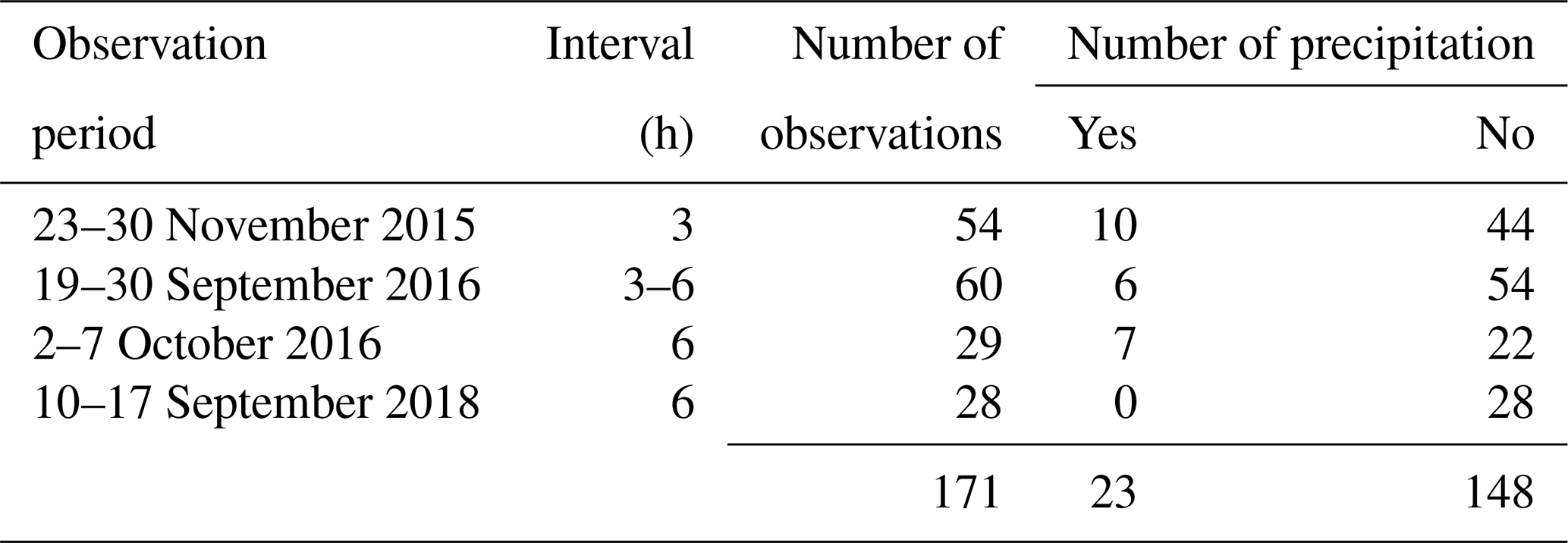
In order to analyze the structure of the atmospheric boundary layer in urban areas, 171 RS sounding data were acquired during the four intensive observation campaigns at Jungnang Station. Because of 23 precipitation cases, 148 RS soundings were used to estimate the ABLH (Table 1). Weather conditions were divided into two categories, i.e., clear sky (cloud cover (CC) ≤30 %) and cloudy sky (CC ≥80 %) for the purpose of investigating the features of the ABLH with respect to weather.

Table 1 Information on GPS radiosonde observations at Jungnang Station in Seoul city, Korea.

3.2 Ceilometer

The backscattering coefficients observed using the ceilometer contain noise, especially near-range artifacts in the lower atmosphere proximate to the lens of the instrument, as well as atmospheric scattering due to intense daytime solar radiation, clouds, and precipitation. The noise can be reduced through the temporal and spatial moving averages of the backscattering coefficients, and they can maintain the vertical and temporal characteristics of backscattering coefficients. Moving average for 10 range gates (100 m) and 10 time steps (10 min) was conducted.

The SNR is introduced to prevent noise from causing the estimation of the ABLH at unreliable heights (de Haij et al., 2006; Heese et al., 2010; Kotthaus et al., 2016). Generally, backscattering coefficients at a higher level than the SNR stop level (h_SNR), the first altitude at which the SNR is less than one, are not used. The SNR at height z is calculated using the formulas introduced by de Haij et al. (2007), as follows:

$$\begin{array}{}\text{(1)}& {\displaystyle }\mathrm{BN}={\displaystyle \frac{\mathrm{1}}{N}}{\sum }_{z=\mathrm{12}\text{km}}^{\mathrm{15}\text{km}}\mathit{\beta }\left(z\right),\text{(2)}& {\displaystyle }{\mathit{\sigma }}_{{\mathit{\beta }}_{\mathrm{SNR}}}=\sqrt{{\displaystyle \frac{\mathrm{1}}{N}}{\sum }_{z=\mathrm{12}\text{km}}^{\mathrm{15}\text{km}}{\left(\mathit{\beta }\left(z\right)-\mathrm{BN}\right)}^{\mathrm{2}}},\text{(3)}& {\displaystyle }\mathrm{SNR}\left(z\right)={\displaystyle \frac{\mathit{\beta }\left(z\right)}{\mathrm{BN}+{\mathit{\sigma }}_{{\mathit{\beta }}_{\mathrm{SNR}}}}},\end{array}$$

where z is the height; β(z) pertains to the backscattering coefficient at z; BN refers to background noise, which is calculated as the mean of β(z) from 12 to 15 km; and N denotes the number of levels between 12 and 15 km (N=300). ${\mathit{\sigma }}_{{\mathit{\beta }}_{\mathrm{SNR}}}$ is the standard deviation of β(z) at altitudes between 12 and 15 km. If the upper layer contains much noise, the SNR of the lower layer becomes smaller, and if the lower air is clean, h_SNR can be distributed in the lowest layer. When the SNR is being calculated, heights above 120 m are used to eliminate the discontinuity due to the instrumental limitation in the lower atmosphere.

Figure 2 shows the comparison of the backscattering coefficients, h_SNR, before and after pre-processing. Strong noises with random backscattering coefficients were found at heights above 2500 m throughout the day (Fig. 2a). When the shortwave radiation was intense during the daytime, the noise was mainly due to sunlit scattering and low SNR values. Especially in the presence of daytime clouds (14:00 to 16:00 LST), the SNR decreased and the h_SNR became lower. Furthermore, the backscattering coefficient is often found to decrease rapidly around 120 and 400 to 500 m high during the daytime with intense solar radiation. It was considered an error in the mechanical instruments or artifacts resulting from the surrounding environment. After pre-processing, noise signals at higher altitude have decreased and maintained their main features (Fig. 2b). But vertical broadening at heights with intense signals was shown as a result of the moving average. And the mean h_SNR became 331 m higher than before. The pre-processing made the values much more stable, although under poor circumstances with strong solar radiation and daytime clouds. Also, artifacts at high altitudes were mitigated.

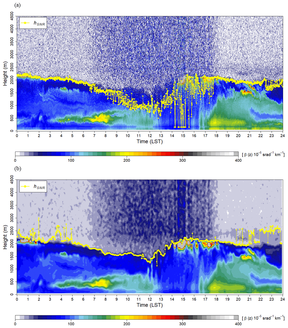
Figure 2 Time–height cross sections of the backscattering coefficient obtained using a ceilometer and signal-to-noise ratio (SNR) stop level (h_SNR) (a) before and (b) after pre-processing.

3.3 Microwave radiometer

The temperature of the MWR and the humidity depend on the generalized atmospheric conditions because they are estimated using an artificial neural network (Collaud Coen et al., 2014). In order to retrieve temperature and humidity with an artificial neural network, a training data set is required. The variables were retrieved using software embedded in the MWR. Given that the neural network cannot guarantee the accuracy of the retrieved data beyond the range of the training data set, the retrieved data include uncertainties. Nevertheless, the SBL formed via surface cooling during nighttime is determined only by the thermal parameter. Cimini et al. (2006) found that most methods had the best performances near the surface and that the bias and standard deviation increased with height. It was also determined that the bias in temperature retrieval is acceptable (<0.5 K) in most methods. The potential temperature calculated by the MWR was used to determine the nocturnal SBLH.

The potential temperature was computed using the vertical profiles of temperature, humidity, and pressure, which were calculated using the ideal gas equation with the assumption of the hydrostatic equation (Holton and Hakim, 2012). The vertical pressure p₂ at z₂ is calculated as follows:

$$\begin{array}{}\text{(4)}& p_{\mathrm{2}}=p_{\mathrm{1}}\exp \left(-g{\displaystyle \frac{z_{\mathrm{2}}-z_{\mathrm{1}}}{R{\stackrel{\mathrm{‾}}{T}}_z}}\right),\end{array}$$

where p₁ is the air pressure z₁ below the z₂, ${\stackrel{\mathrm{‾}}{T}}_z$ pertains to the mean temperature between z₁ and z₂, R refers to the gas constant for air (287 J kg⁻¹ K⁻¹), and g denotes the gravitational acceleration. The potential temperature is calculated using the following equation:

$$\begin{array}{}\text{(5)}& {\mathit{\theta }}_z=T_z{\left({\displaystyle \frac{p_{\mathrm{0}}}{p_z}}\right)}^{\frac{R}{c_{\mathrm{p}}}},\end{array}$$

where θ_z is the potential temperature at height z, and p₀ and p_z are the air pressures at the 1000 hPa level and height z, respectively. Moreover, c_p pertains to the specific heat of dry air at constant pressure (1004 J kg⁻¹ K⁻¹).

4 Methodology

4.1 Review of the ABLH estimation method using radiosonde

A parcel method, a gradient method, and a bulk Richardson number method can be considered to estimate the ABLH using the sounding data obtained via radiosonde. Among them, the bulk Richardson number method was used to determine the reference ABLH. The bulk Richardson number (Ri_b) is defined as the ratio of buoyancy forcing vis-à-vis mechanical forcing by vertical wind shear:

$$\begin{array}{}\text{(6)}& R{i}_{\mathrm{b}}={\displaystyle \frac{\left(g/\phantom{g{\mathit{\theta }}_{\mathrm{0}}}{\mathit{\theta }}_{\mathrm{0}}\right)({\mathit{\theta }}_z-{\mathit{\theta }}_{\mathrm{0}})}{{u_z}^{\mathrm{2}}+{v_z}^{\mathrm{2}}}}z,\end{array}$$

where z is the height, u_z and v_z are the west–east and south–north wind speeds at z, respectively, θ₀ pertains to the surface potential temperature, and θ_z refers to the potential temperature at z. According to Stull (1988), laboratory research suggested that turbulence occurs when Ri is smaller than the critical Ri, Ri_c. Many previous studies have reported Ri_c values between 0.1 and 1.0 (e.g., Holtslag and Boville, 1993; Jeričević and Grisogono, 2006; and Esau and Zilitinkevich, 2010). The values of 0.25 and 0.5 were the most utilized Ri_c (Zhang et al., 2014). In this study, we used a value of 0.5 for the Ri_c.

In order to determine the ABLH in the case of stable stratification, Collaud Coen et al. (2014) determined the nocturnal SBLH using the temperature and potential temperature profiles from the radiosonde and MWR. SBLH is determined as a surface-based temperature inversion (SBI) height at which the temperature decreases with height (ΔT∕Δz<0) for the first time (Stull, 1988; Seidel et al., 2010). Actually, it is not easy to detect a SBLH using RS sounding. This is because the vertical variations of the temperature and the wind in the RL can be more substantial compared to those in the SBL. Thus, the SBLH has been generally estimated using the methodologies with temperature inversion. In this study, the ABLHs were estimated with Ri_b in both daytime and nighttime, and if a SBL was formed at nighttime, the SBLHs were determined via the SBI method. Nonetheless, the top of the RL is still determined as a SBLH due to the large variation of temperature and turbulence (Collaud Coen et al., 2014).

4.2 Review of the ABLH estimation method using a ceilometer

4.2.1 Time-variance method

The time-variance method (VAR) computes for the standard deviation (${\mathit{\sigma }}_{{\mathit{\beta }}_{(z,t)}}$) of the backscattering coefficient profile measured by the ceilometer for 10 min using Eq. (7).

$$\begin{array}{}\text{(7)}& {\displaystyle }{\mathit{\sigma }}_{{\mathit{\beta }}_{\mathrm{VAR}}}=\sqrt{{\displaystyle \frac{\mathrm{1}}{N}}{\sum }_{t=\mathrm{1}}^N{\left(\mathit{\beta }(z,t)-\stackrel{\mathrm{‾}}{\mathit{\beta }(z,t)}\right)}^{\mathrm{2}}},\text{(8)}& {\displaystyle }{h}_{\mathrm{VAR}}=\max \left({\mathit{\sigma }}_{{\mathit{\beta }}_{\mathrm{VAR}}}\right),z\mathit{<}{h}_{\mathrm{SNR}},\end{array}$$

where β(z,t) is the backscattering coefficient profile at time t, $\stackrel{\mathrm{‾}}{\mathit{\beta }(z,t)}$ pertains to the 10 min mean backscattering coefficient, and N refers to the number of profiles (in this study, N=10). ${\mathit{\sigma }}_{{\mathit{\beta }}_{\mathrm{VAR}}}$ represents the peak at high temporal variability, and thus the ABLH estimated by VAR (h_VAR) is determined as the height at which ${\mathit{\sigma }}_{{\mathit{\beta }}_{\mathrm{VAR}}}$ shows a maximum value, which is less than h_SNR (1480 m). The ${\mathit{\sigma }}_{{\mathit{\beta }}_{\mathrm{VAR}}}$ profile was smoothed using a local quadratic polynomial regression (Cleveland and Loader, 1996) to eliminate spurious variance peaks at small-scale fluctuations. Nevertheless, σ_β(z,t) contains a spurious peak above h_SNR and gradually increases with height. For the foregoing reasons, h_VAR was calculated only below h_SNR.

Figure 3a shows the profiles of the ${\mathit{\sigma }}_{{\mathit{\beta }}_{\mathrm{VAR}}}$ (red line), $\stackrel{\mathrm{‾}}{\mathit{\beta }(z,t)}$ (black line), and β(z,t) at intervals of 1 min (dashed gray line) for 10:50 to 11:00 LST on 23 September 2016, and the ABLH was determined by VAR (h_VAR=670 m).

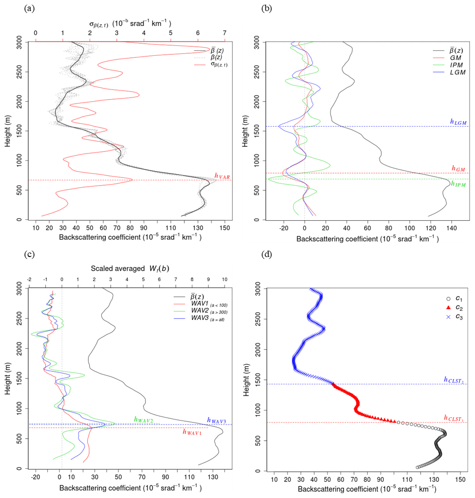
Figure 3 Examples of ABLH estimations. (a) Time-variance method: 10 min averaged β_(z) (bold black line) and standard deviation (${\mathit{\sigma }}_{{\mathit{\beta }}_{(z,t)}}$) (red line) at 11:00 LST on 23 September 2016; the gray curves are β_(z) at intervals of 1 min from 10:50 to 11:00 LST; h_VAR is the ABLH retrieved by the time-variance method. (b) Gradient method (GM, IPM, LGM): the bold black line indicates the 10 min averaged β_(z), while the thin solid, dashed, and dash-dotted lines indicate the GM, IPM, and LGM, respectively; the ABLHs ($h_{\mathrm{GM}},h_{\mathrm{IMP}},h_{\mathrm{IPM}}$) are determined via each method. (c) Wavelet covariance transform method (WAV): the bold black line indicates the 10 min averaged β_(z), while the thin solid, dashed, and dash-dotted lines indicate that of WAV1, 2, and 3, respectively; and h_WAV1, h_WAV2, and h_WAV3 denote ABLHs, the peaks in each WAV profile. (d) The k-means clustering analysis method: black circles, red triangles, and blue “×” marks represent the different clusters, while the boundaries of the clusters (h_CLST1, h_CLST2) denote the ABLH.

4.2.2 Gradient method

The gradient method is one of the most commonly used methodologies for estimating ABLH. The maximum negative peak of the first derivative with respect to the height of the backscattering coefficient from the ceilometer was determined as the ABLH. Generally, the first derivative (GM: gradient method), second derivative (IPM: inflection point method), and logarithmic derivative (LGM: logarithmic gradient method) are used, and the equations are shown below:

$$\begin{array}{}\text{(9)}& {\displaystyle }{h}_{\mathrm{GM}}=\min \left({\displaystyle \frac{\partial \mathit{\beta }\left(z\right)}{\partial z}}\right),\text{(10)}& {\displaystyle }{h}_{\mathrm{IPM}}=\min \left({\displaystyle \frac{{\partial }^{\mathrm{2}}\mathit{\beta }\left(z\right)}{\partial z^{\mathrm{2}}}}\right),\text{(11)}& {\displaystyle }{h}_{\mathrm{LGM}}=\min \left({\displaystyle \frac{\partial \ln \mathit{\beta }\left(z\right)}{\partial z}}\right).\end{array}$$

Figure 3b shows the results of the gradient methods corresponding to 11:00 LST on 23 September 2016. The bold solid line is a smoothed β(z) profile, while the GM, IPM, and LGM results are represented by the solid, dotted, and dash-dotted lines, respectively. h_GM, h_IPM, and h_LGM indicate ABLH with a maximum negative gradient for each method. The value of h_GM (790 m) is slightly higher than that of h_IPM (690 m) and lower than that of h_LGM (1580 m). The fact that h_GM is slightly higher than h_IPM and lower than h_LGM is consistent with the findings of previous studies (e.g., Emeis et al., 2008). The second-largest negative (800 m) in the LGM was similar to h_GM, and the second-largest negative in GM (1570 m) was also similar to the h_LGM height. The h_IPM is similar to h_VAR (670 m), and both are located at an altitude where β(z) begins to decrease sharply. Notwithstanding that the altitude at which the maximum negative gradient for each method can be different, they can be similar to the altitude corresponding to the second peaks for other methods.

4.2.3 Wavelet covariance transform method

The wavelet covariance transform method (WAV) is also one of the most commonly used methods. The WAV uses the Haar step function, which is defined as follows:

$$\begin{array}{}\text{(12)}& h\left({\displaystyle \frac{z-b}{a}}\right)=\left\{\begin{array}{l}+\mathrm{1}:b-\frac{a}{\mathrm{2}}\le z\le b\\ -\mathrm{1}:b\le z\le b+\frac{a}{\mathrm{2}}\\ \mathrm{0}:\mathrm{elsewhere}\end{array}\right.,\end{array}$$

where b is the translation of the function (the location at which the function is centered), and a pertains to the dilation of the function (the spatial extent). The covariance transform of the Haar function, W_β, is defined as follows:

$$\begin{array}{}\text{(13)}& {\displaystyle }{W}_{\mathit{\beta }}(a,b)={\displaystyle \frac{\mathrm{1}}{a}}{\int }_{z_{\mathrm{b}}}^{z_{\mathrm{t}}}\mathit{\beta }\left(z\right)h\left({\displaystyle \frac{z-b}{a}}\right)\mathrm{d}z,\text{(14)}& {\displaystyle }{h}_{\mathrm{WAV}}=\max \left(W_{\mathit{\beta }}\right(a,b\left)\right),\end{array}$$

where z_b and z_t are the bottom and top heights of the profile, respectively. The altitude with the maximum value of W_β(a,b) is determined using ABLH (h_WAV). In this study, a is set to 24 dilations at intervals of 15 m from 15 to 360 m, while b is set to 10 m step size from 60 to 3000 m (de Haij et al., 2006, 2007).

Davis et al. (2000) illustrated the importance of determining the dilation through experiments that used the airborne lidar backscattering profile. Smaller dilations are sensitive to small-scale fluctuations of β(z) and are inclined to include noise, while larger dilations tend to ignore small-scale structures and detect changes in scale, such as the entrainment zone. Especially in the real atmosphere, small-scale fluctuation of β(z) due to sudden turbulence appears, and it plays an important role in mechanical mixing in ML. In order to consider small-scale features, W_β(a,b) profiles were processed by averaging over a<100 m (WAV1), a>300 m (WAV2), and the total a (WAV3) (de Haij et al., 2007). The height with the maximum values of W_β(a,b) by WAV1, WAV2, and WAV3 can be determined as the ABLH (h_WAV1, h_WAV2, h_WAV3), respectively.

Figure 3c shows the results of the wavelet method. The bold solid line is a smoothed β(z), while the solid, dashed, and dash-dotted lines indicate the results of WAV1, WAV2, and WAV3, respectively. As described in Sect. 4.2.2, β(z) decreases rapidly at altitudes of approximately 700 and 1500 m, while W_β(a,b) peaks at very close altitudes. In WAV1, the first peak (h_WAV1) appeared at 680 m, which is very close to h_VAR (670 m) and h_IMP (690 m). WAV2 (WAV3) showed two peaks at 750 m (730 m) and 1550 m (1550 m). The first peaks (h_WAV2, h_WAV3) were similar to h_GM (790 m), and the second peaks were similar to h_LGM (1580 m; second peak of h_GM).

4.2.4 Clustering analysis method

The k-means clustering analysis (CLST) is a nonhierarchical clustering method that can determine the ABLH by dividing the height where the backscattering coefficient profile from the ceilometer sharply decreases or increases. The cluster center is applied to the backscattering coefficient to minimize the sum of the squared errors (Toledo et al., 2014). The number of cluster seeds was determined using the Dunn index (Dunn, 1974; Toledo et al., 2014).

Figure 3d shows the ABLH estimation results using the k-means clustering analysis method at 11:00 LST on 23 September 2016. As a result of the cluster validation, the optimal number calculated by the Dunn index was three, and the clusters were distinguished at 800 m (h_CLST1) and 1430 m (h_CLST2). The altitude at which a cluster changes to another cluster can be determined as the ABLH. The values of h_CLST1 were similar to those of h_GM (790 m) and h_WAV1 (770 m). h_CLST2 was slightly lower than h_LGM (1580 m) and h_WAV2 (1530 m).

4.3 Nocturnal SBLH estimation using a microwave radiometer

It is possible to estimate the nocturnal SBLH by determining the thermal stability and instability from the microwave-radiometer-derived vertical profiles of thermal parameters, such as temperature and potential temperature (Collaud Coen et al., 2014; Saeed et al., 2016). Given the vertical profile of the atmospheric temperature, it is possible to determine the altitude of d$T/\mathrm{d}z=\mathrm{0}$ according to the SBI method for the purpose of establishing the thermal stability. However, in real atmospheric conditions, the air parcel follows the environmental lapse rate (ELR), which differs depending on the time and place rather than the theoretical lapse rate (TLR), and the criterion of the potential temperature gradient is also dominant in the ELR. In this study, it is assumed that there is a high possibility that SBL (dθ∕dz) exists near the surface to be larger than the ELR. After that, we set the threshold (${\stackrel{\mathrm{‾}}{\mathrm{\Gamma }}}_f$) of the ELR, taking into consideration the vertical variability of dθ∕dz to distinguish the distinct layers.

Figure 4a and b show the vertical profiles of the potential temperature and the vertical gradient of the potential temperature obtained by a MWR at Jungnang Station at 15:00 LST (solid line) and 21:00 LST (dashed line) on 23 September 2016, as well as 00:00 LST (dotted line) on 24 September 2016. The potential temperature decreases with height at a constant rate above 2000 m (Fig. 4a), and it can be considered a slope of the ELR. The TLR and ELR are shown in Fig. 4b as solid and dashed gray lines, respectively. It was thermally unstable at 15:00 LST on 23 September 2016 when the value near the surface was smaller than the TLR (Fig. 4b). As the near-surface temperature decreased due to surface cooling after sunset and a stable layer with a positive value of dθ∕dz appeared, the slope of dθ∕dz increased and a more stable layer was formed at 00:00 LST on 24 September 2016. At this time, the daily mean potential temperature gradient in the free atmosphere over 2000 m was 5.5 K km⁻¹, and this value is used as the threshold (${\stackrel{\mathrm{‾}}{\mathrm{\Gamma }}}_f$) for the ELR.

Figure 4 Vertical profiles of (a) potential temperature, (b) gradient of potential temperature, (c) vertical variances of dθ∕dz at 15:00 LST (solid line) and 21:00 LST (dashed line) on 23 September 2016, as well as 00:00 LST (dotted line) on 24 September 2016. The vertical lines in panel (b) denote the theoretical lapse rate (solid gray line) and the environmental lapse rate (dashed gray line). The gray line denotes the altitude at which the vertical variance at 00:00 LST on 24 September 2016 decreases sharply.

Thus, it can be concluded that the layer is considered as a stably affecting layer if dθ∕dz is greater than ${\stackrel{\mathrm{‾}}{\mathrm{\Gamma }}}_f$ and an unstably affecting layer if dθ∕dz is smaller than ${\stackrel{\mathrm{‾}}{\mathrm{\Gamma }}}_f$. The dθ∕dz in the lower atmosphere at 21:00 LST on 23 September 2016 is greater than 0 K km⁻¹, which is the stable condition in the TLR criterion; however, it was smaller than 5.5 K km⁻¹. Therefore, it is difficult to determine it as stable in the ELR. Figure 4c shows the vertical variance of dθ∕dz. The vertical variance was calculated for 150 m at each altitude. At 15:00 LST on 23 September 2016, which was well mixed vertically, the variance of dθ∕dz in the lower atmosphere was close to 0 K km⁻¹, whereas there was a significant variance of dθ∕dz at 21:00 LST on 23 and 00:00 LST on 24 September 2016. It is possible to determine the altitude at which the vertical variance decreases rapidly (500 m; gray line in Fig. 4b) at 00:00 LST on 24 September 2016, satisfying the ELR condition, and dθ∕dz at an altitude of 3.6 K km⁻¹.

Since both ${\stackrel{\mathrm{‾}}{\mathrm{\Gamma }}}_f$ and dθ∕dz depend on time, we determined the altitude at which the vertical variance of the daily data decreases sharply every 10 min while satisfying the stable ELR condition ($\mathit{>}{\stackrel{\mathrm{‾}}{\mathrm{\Gamma }}}_f$) for threshold setting. With regard to the distinct layer classification, the altitude of the maximum vertical variance during a day and the potential temperature gradient of that day as the critical lapse rate of that day (CLR Γ_cr) were determined.

$$\begin{array}{}\text{(15)}& {\displaystyle }\mathrm{Var}{\left({\displaystyle \frac{\partial \mathit{\theta }}{\partial z}}\right)}_z={\displaystyle \frac{\mathrm{1}}{H}}{\sum }_{z=\mathrm{1}}^H{\left[{\left({\displaystyle \frac{\partial \mathit{\theta }}{\partial z}}\right)}_z-{\left(\overline{{\displaystyle \frac{\partial \mathit{\theta }}{\partial z}}}\right)}_z\right]}^{\mathrm{2}},\text{(16)}& {\displaystyle }{\mathrm{\Gamma }}_{\mathrm{cr}}=\begin{array}{c}max\\ t=\mathrm{1}\mathrm{d}\end{array}\left\{max{\left(\mathrm{Var}\left({\displaystyle \frac{\partial \mathit{\theta }}{\partial z}}\right)\right)}_t\right\},\end{array}$$

where $\mathrm{Var}{\left(\frac{\partial \mathit{\theta }}{\partial z}\right)}_z$ is the vertical variance of the potential temperature gradient at z height, ${\left(\frac{\partial \mathit{\theta }}{\partial z}\right)}_z$ pertains to the potential temperature gradient at z height, ${\left(\frac{\overline{\partial \mathit{\theta }}}{\partial z}\right)}_z$ represents the mean potential temperature gradient over ±150 m at z height, and H denotes the number of vertical intervals (H=6; 300 m).

As a result, on 23 September 2016, Γ_cr was 7.0 K km⁻¹, and the altitude at which the dθ∕dz profile crosses CLR was determined as SBLH. In order to improve the quality of the MWR data, surface heating via shortwave radiation (net radiation >0 W m⁻²) and precipitation were removed.

During the radiosonde intensive observation period, only four SBL cases were detected using the SBI methodology from the radiosonde. The SBLH via the SBI method was compared with that obtained using the CLR method. Figure 5 shows the vertical profile of the potential temperature gradient, threshold of lapse rate (Γ_cr), and SBLH estimated using each methodology, i.e., SBI using the radiosonde (RS_SBI), SBI using the MWR (MWR_SBI), and CLR using the MWR (MWR_CLR). SBLHs were estimated at the same time using the radiosonde and MWR (Fig. 5a to c). In case of Fig. 5d, the MWR showed SBL an hour later (01:00 LST). The MWR_SBI was estimated to be lower than MWR_CLR and only when the atmosphere condition was markedly stable (Fig. 5b, c). In this study, the CLR method was applied to estimate SBLH using the MWR, which estimates SBLH more accurately and stably.

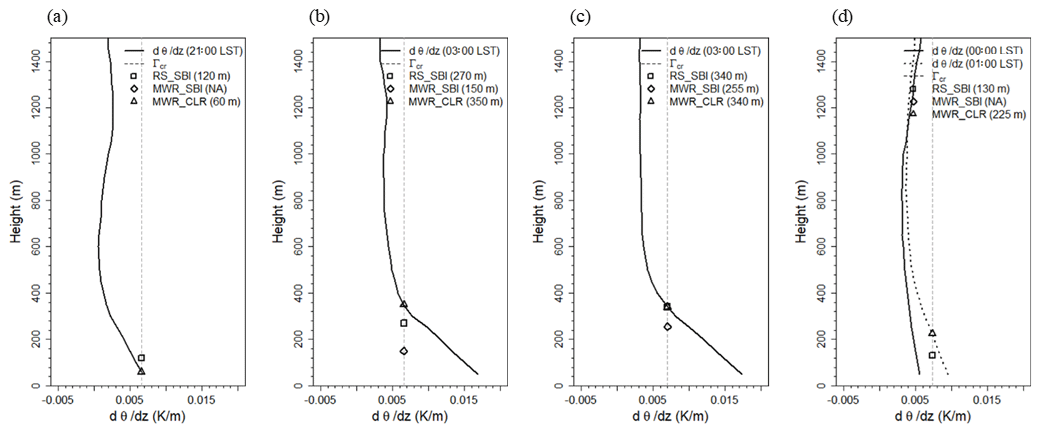
Figure 5 Vertical profiles of potential temperature, threshold of lapse rate (Γ_cr), and the SBLHs estimated by the radiosonde and the MWR at (a) 21:00 LST on 22 September 2016, (b) 03:00 LST on 23 September 2016, (c) 03:00 LST on 24 September 2016, and (d) 00:00 LST on 27 September 2016. The SBI method was applied to two measurements (RS_SBI, MWR_SBI), while the CLR method was applied to the MWR (MWR_CLR).

4.4 Integrated system for ABLH estimation

In a real atmosphere, there is not only one ABL but a complicated structure with several layers that are dependent on time, place, and atmospheric phenomena. Therefore, ABLH shows differences among methodologies and is an arbitrary decision by the researcher. In this study, an integrated system for ABLH estimation (ISABLE) was developed to determine the optimal ABLH. ISABLE applies the four methodologies described above using the backscattering coefficient from the ceilometer as well as the CLR method that uses the potential temperature profiles from the MWR.

4.4.1 Integration method

Figure 6 shows the schematic flow of the ABLH candidate group selection process. INPUT is the ABLH estimated by applying the four methods using a backscattering coefficient from the ceilometer, and in the present study, it was estimated to be up to 19 layers. The VAR selects a maximum of three peaks as ABLH candidates. In the GM, a maximum of five peaks are found to minimize redundancy at the chosen level. In the WAV method, up to three altitudes are selected as ABLH candidates for WAV3 considering the full dilation, and WAV1 and WAV2 select two altitudes to minimize the redundancy to WAV3. The CLST selected a maximum of four altitudes to remove the possible noise structure. The minimum distance between the nearest two ABLH candidates was set to 150 m. The reason is that the typical thickness of a well-defined entrainment zone was reported to be between 100 and 300 m (Angevine et al., 1994). If there were multiple peaks chosen using each methodology within a 150 m interval, the remaining peaks except for the most significant one were removed from the ABLH candidates for the method.

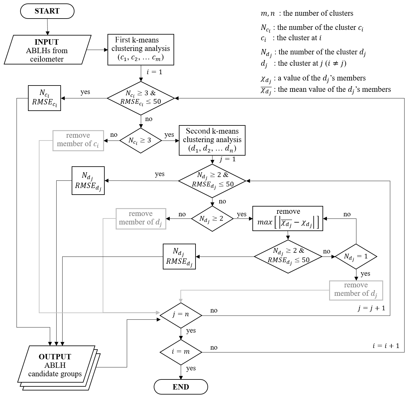
Figure 6 Flowchart of the algorithm for ABLH estimation from the vertical profile of the backscattering coefficient obtained using a ceilometer.

The ABLH candidate groups were selected via the k-means clustering analysis method for the maximum of 19 ABLHs. Through the first clustering, groups with three or more members and RMSE less than or equal to 50 m are classified into the ABLH candidate groups. If the number of members is less than three and the RMSE is higher than 50 m, the member is excluded from the ABLH candidate groups. If the number of members is greater than or equal to three but the RMSE exceeds 50 m, a second clustering analysis is performed.

The second clustering analysis on members of the undetermined candidate group is performed such that if the number of members is greater than or equal to two and the RMSE is less than 50 m, the group is classified into the ABLH candidate groups. If the number of members is less than two, the members are removed; if the number of members is greater than or equal to two and the RMSE exceeds 50 m, the member with the farthest distance from the mean of the group is removed. The foregoing procedure is repeated until the number of members is greater than or equal to two and the RMSE does not exceed 50 m. Thereafter, the last group is classified as an ABLH candidate group.

The final OUTPUT, the ABLH candidate groups, is ranked in descending order of the number of members, and if the number of members is the same, the RMSE is ranked in ascending order. Up to five groups were selected, and the average of each group was determined as the final ABLHs estimated by the ceilometer backscattering coefficient. If the SBLH is observed by the MWR, it is added to the final ABLHs.

4.4.2 ISABLE post-processing

Various ABLH estimation methodologies have been merged with ISABLE. However, there are still limitations in terms of estimating the ABLH, such as observational errors and small-scale fluctuations in a real atmosphere, and the appropriate post-processing, which is required as per Kotthaus and Grimmond (2018). Unreasonable ABLHs, such as the ABLH above h_SNR, and near-range artifacts caused by instrument-related and isolated ABLH-related small-scale structures are removed through the three-step post-process.

Figure 7a shows the ABLHs determined by ceilometer observations without post-processing (CM_ABLH) from 18:00 LST on 22 September 2016 to 12:00 LST on 25 September 2016. There are not only ABLHs higher than h_SNR within the range of 10:00 to 12:00 LST on 25 September 2016, but also near-range ABLHs in the daytime (12:00 to 16:00 LST) when the convective is well developed, and isolated ABLHs that seem independent without time–space continuity are formed. First, the ABLHs that are higher than h_SNR are removed. As a result, the ABLHs that appeared at approximately 2500 m within 10:00 to 12:00 LST on 25 September 2016 were removed (Fig. 7b). As mentioned in Sect. 3.2, the altitude higher than h_SNR contained less meaningful information because the backscatter signal, as compared with the background noise, is weak. Second, the ABLHs in the lower atmosphere during the daytime, represented by the near-range artifacts, were removed (Fig. 7c). The ABLH grows slowly after sunrise, while it overgrows approximately 1 to 2 h before noon. The maximum ABLH appears approximately 2 to 3 h after noon (14:00 to 16:00 LST). During this period, vertical mixing through convection is active due to surface heating, and thus the ABLH grows to the maximum. Therefore, the ABLH that appears in the lower layer at the time might be inappropriate due to instrumental noise or near-range artifacts. Using the radiation observation at Jungnang Station, the convective mixing period was set from 1 h before the time of maximum net radiation to 1 h after sunset (the net radiation is 0 W m⁻²). It was found that backscattering signals were weakened at about 120 m and 400 to 500 m high, respectively, during the daytime with intense solar radiation (Fig. 2a). Due to the weakened signal, the 400 to 500 m could be often estimated as an ABLH. So, ABLHs below 500 m at the time were assumed to be unreasonable and were neglected (Fig. 7b). Third, in order to find the discontinuous ABLH caused by small-scale fluctuations and a separated small-scale aerosol layer, the ABLH is assumed to be discontinuous if no other ABLHs are present within ±10 time steps (100 min) and ±12 range gates (120 m). Additionally, the density-based spatial clustering of applications with noise (DBSCAN; Ester et al., 1996) can eliminate isolated ABLHs. DBSCAN is an algorithm that extracts the noise contained in a cluster. Each point (core point) of a cluster and neighborhoods (border points) within a given radius (ε) must contain a minimum number of points (MinPts) within ε. In order to apply the same ε to the time–height axes, DBSCAN is performed on a normalized ABLH with values between 0 and 1. Figure 7d shows the result of the discontinuity check using DBSCAN with ε=0.0125 (t=72 min; z=56 m) and MinPts = 3. The discontinuous and sole ABLHs were removed, and the boundary layer distinction became more pronounced.

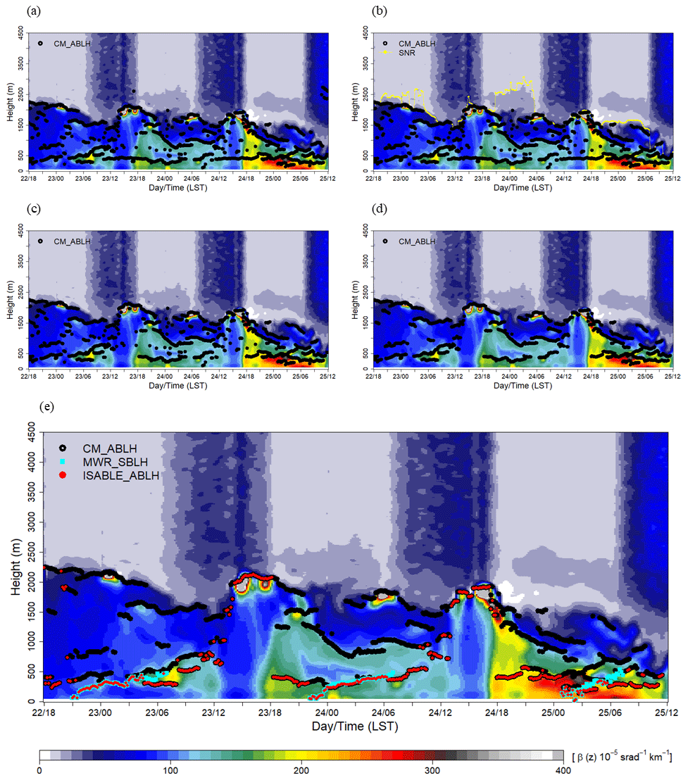
Figure 7 Post-processing steps for determining the ABLH by ISABLE (ISABLE_ABLH): (a) time series of the ABLH (CM_ABLH) without quality control; (b) applying h_SNR threshold height and eliminating unreasonable values near the lens of the ceilometer; (c) removing isolated ABLH using temporal discontinuity and DBSCAN; (d) the SBLHs estimated via microwave radiometer (MWR_SBLH) were merged and then post-processing was applied; (e) final ABLHs were used to determine the lowest layer.

Figure 7e shows the backscattering coefficient and CM_ABLH from those after post-processing. In addition, the nocturnal SBLH estimated using a microwave radiometer (MWR_ABLH) was merged with the CM_ABLH. Finally, the ABLHs determined via ISABLE (ISABLE_ABLH) were determined as the lowest of the remaining CM_ABLHs and MWR_ABLH.

5 Results

5.1 Diurnal variation of the ABLH from radiosonde

ABLHs were calculated using the 148 radiosonde observations launched at the Jungnang Station in Seoul from 2015 to 2018. Figure 8 shows the diurnal variation of the ABLH. The ABLH estimated using radiosonde exhibited a maximum at 15:00 LST (mean = 1019 m, median = 925 m) and a minimum at 06:00 LST (mean = 418 m, median = 250 m). At night, the mean ABLHs were determined as around 500 m, and outliers appeared above 1 km, which were identified as the RL or clouds (Fig. 8). The interquartile range (IQR; Q3–Q1) showed the minimum value (268 m) at 09:00 LST and the maximum (740 m) at 18:00 LST. Overall, ABLHs were concentrated in the lower layer at night, and the IQR values increased as the ML developed after sunrise.

Figure 8 Box plot of 3 h interval ABLHs estimated using the 148 radiosondes observed at Jungnang Station from 2015 to 2018. The rhombus is the mean ABLH, the dots are outliers, and the gray crosses represent the 10th and 90th percentiles, respectively. IQR implies an interquartile range. The numbers at the top indicate the data frequency.

The SBL over rural areas such as a grass field or crop field is well developed due to active radiative cooling at night, especially under clear skies. In contrast, the radiative cooling over urban areas was not always active because of heat storage by urban materials and anthropogenic heat by energy use (Hong et al., 2013; Park et al., 2014). As a result, formation and evolution of SBL were not active over dense urban areas such as Jungnang Station.

5.2 ISABLE performance assessment

Figure 9 shows the ABLHs obtained by radiosonde observation (RS), the ISABLE algorithm, and the results of each methodology obtained using a ceilometer and a MWR from 18:00 LST on 22 September 2016 to 12:00 LST on 25 September 2016. The period corresponds to the longest observation period with an interval of 3 h and without any missing data among available RS data. The same diurnal variation was observed in the RS and ISABLE results. The correlation coefficient (R) between the two exhibited a high correlation of 0.98, with a mean bias (MB) of −101 m and a root mean square error (RMSE) of 135 m. The ABLHs from ISABLE as well as ceilometer-based methods (GM, WAV2, WAV3, and CLST) were similar to those by RS during the daytime; however, the ABLHs from the former appeared at higher levels than those from the latter during the nighttime. This might be mainly due to the more significant signal in the RL. ISABLE tried to complement the shortcomings by integrating the four methodologies through considering the SBL using a vertical temperature from MWR at night. The maximum ABLHs during daytime appeared at 16:00 LST on 23 September 2016, and the RS and the ISABLE algorithm estimated ABLHs of 1620 and 2009 m, respectively. At this time, a cumulus cloud was formed over the top of the ABL due to strong convection, and the cloud base height observed by the ceilometer was 1910 m. The ABLH estimation results showed that RS was below the cloud, while ISABLE and individual methodologies (GM: 2080 m, WAV2: 2060 m, WAV3: 2050 m) detected ABLHs as the cloud. In the presence of clouds, the Ri_b method tends to detect the base of the cloud layer, where the temperature profile changes rapidly. The GM and WAV2 methods using the ceilometer determine the ABLHs as the top of the layer because of the strong negative gradient of the backscattering coefficient, whereas the CLST can detect both the base and top of the cloud layer. In ISABLE, the effect of clouds is compensated for by averaging multiple heights determined by individual methodologies. However, the ISABLE algorithm still has limitations in the presence of thick clouds.

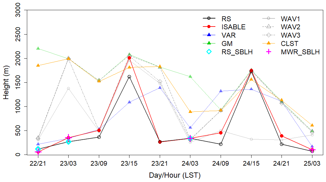
Figure 9 Time series of the ABLH estimated via radiosonde, ISABLE, VAR, GM, WAV1, WAV2, WAV3, and CLST methodologies from 21:00 LST on 22 September 2016 to 03:00 LST on 25 September 2016. The SBLHs, estimated via radiosonde (RS_SBLH) and microwave radiometer (MWR_SBLH), are indicated at nighttime.

Table 2 shows the performance of the ABLHs estimated by ISABLE and the four methodologies with respect to the ABLH determined using the Ri_b calculated via RS. Moreover, Fig. 10 shows the scatter plots of ABLHs estimated via RS and ceilometer/MWR (WAV1 and 3 are not included). The total RSs (number of data sets: 148) were classified into four time zones: i.e., near sunrise (N=47; 06:00 to 11:00 LST), daytime (N=31; 12:00 to 17:00 LST), near sunset (N=34; 18:00 to 22:00 LST), and nighttime (N=36; 23:00 to 05:00 LST). The correlation coefficient between the ABLHs of RS and ISABLE for the entire period was 0.72, MB was −34 m, and RMSE was 322 m. With regard to the individual methodologies, VAR exhibited the best performance (R=0.60; MB = 219 m; RMSE = 372 m), and CLST exhibited the second best performance (R=0.45; MB = 125 m; RMSE = 474 m). These two methodologies showed the best performances during the daytime. The scatter distribution of GM, WAV2, and CLST at sunrise, sunset, and nighttime could be fitted to two groups with different linear functions. In cases where symbols were plotted below the trend line (dashed line), RLs during nighttime or cloud layers in daytime existed at the layer. ISABLE (Fig. 10e) showed significant improvement near sunrise and sunset time but showed a lower correlation with the individual methodologies in nighttime because the ABLH was often underestimated, as compared with RS. There were only four SBLH estimations via RS, while 24 SBLHs were observed via MWR, which resulted in significantly lower ISABLE performance at nighttime, as compared with those of the four methodologies. Overestimation of RS_ABLHs could lead to an underestimation of ABLHs. Anthropogenic heat release from urban materials could be one reason for detecting a lower number of SBLHs at night (Hong et al., 2013; Park et al., 2014). Further analysis is required in considering the accuracy and uncertainty of the two instruments as well as the effects of urban heat islands. The performances of WAV1 and WAV3 were significantly poorer than those of other individual methodologies. The shorter dilation (a<100 m) used in WAV1 seems to be unsuitable for estimating the ABLH, and it might affect the ABLH of WAV3.

Table 2 Statistical performance between ABLHs obtained by various methods, including ISABLE and radiosonde observations for all data (N=148), sunrise (N=47; 06:00 to 11:00 LST), daytime (N=31; 12:00 to 17:00 LST), sunset (N=34; 18:00 to 22:00 LST), and nighttime (N=36; 23:00 to 05:00 LST).

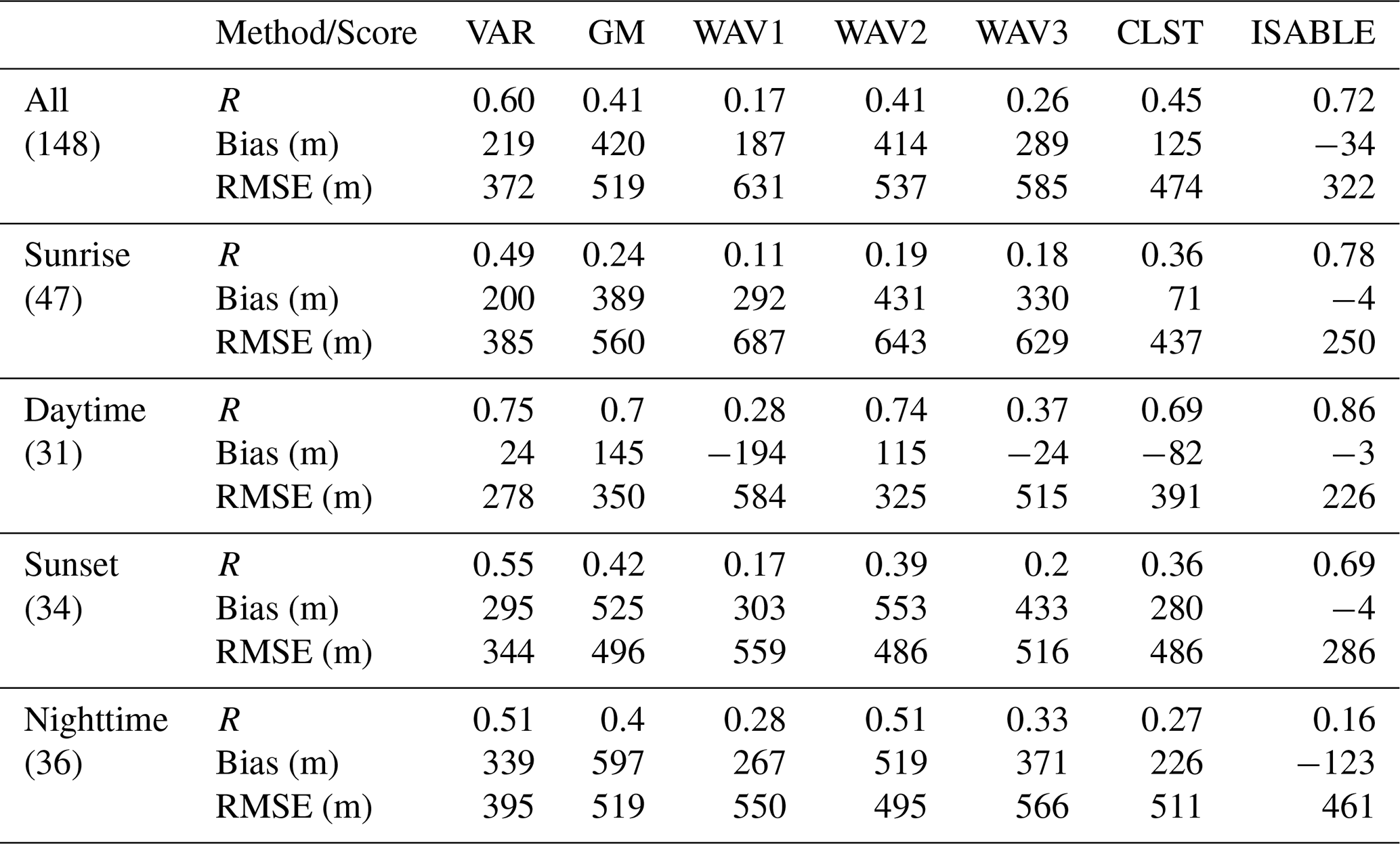
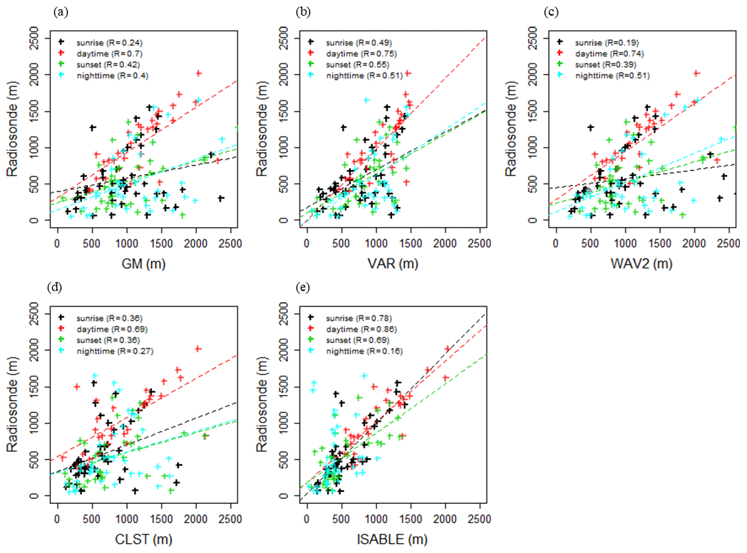
Figure 10 Comparison of ABLH (m) estimates using ISABLE with ABLH estimated via (a) GM, (b) VAR, (c) WAV2, (d) CLST, and (e) ISABLE for sunrise time (N=47; 06:00 to 11:00 LST), daytime (N=31; 12:00 to 17:00 LST), sunset time (N=34; 18:00 to 22:00 LST), and nighttime (N=36; 23:00 to 05:00 LST). The numbers in parentheses represent the correlation coefficients.

Table 3 and Fig. 11 show the performances of the ABLHs via ceilometer/MWR and the scatter plots between two ABLHs for two categories of clear (N=36; CC ≤ 30 %) and cloudy (N=26; CC ≥ 80 %) skies. The foregoing analysis is made with the use of data from 2016 to 2018 due to the availability of cloud cover data. GM and WAV2 were found to show lower verification scores in clear-sky cases in previous studies. This is mainly because the GM and WAV2 methods tend to determine the altitude of clouds or RL. As a result, even in Fig. 11, scatter plots could be fitted to two groups with different linear lines, and the resulting performance scores decreased. Most deviations were related to the RL at nighttime. In order to reduce the deviation in GM and WAV2, ISABLE statistically integrates up to five candidates of the ABLHs estimated from four methodologies and is set to determine the lowest candidate as the final ABLH so that it could detect the height below the RL or cloud base.

Table 3 Statistical performance between ABLHs obtained by various methods, including ISABLE and radiosonde observations for clear (N=36; CC ≤ 30 %) and cloudy skies (N=26; CC ≥ 80 %) for the period from August 2016 to October 2018.

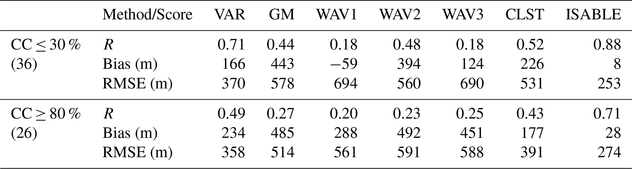
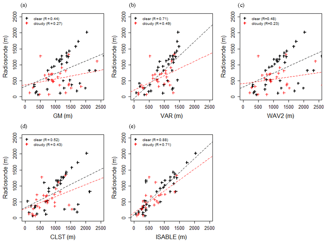
Figure 11 The same as Fig. 10, except that the data herein pertain to clear-sky cases (N=36; CC ≤ 30 %) and cloudy-sky cases (N=26; CC ≥ 80 %).

The MB and RMSE for nocturnal SBLH were as good as 6.7 and 72 m, respectively, although the number of available data were not sufficient.

5.3 Diurnal and seasonal variations in ABLH from ISABLE

For the period from August 2016 to October 2018, the ISABLE ABLH was determined using the vertical profiles of the backscattering coefficient from the ceilometer and potential temperature from the MWR at Jungnang Station in Seoul. Unfortunately, cloud cover from 2015 to July 2016 was not observed, and the period was excluded from the analysis. Figure 12 shows the diurnal variations over the observation period of clear (Fig. 12a) and cloudy (Fig. 12b) skies. The period mean hourly ABLHs were high in the clear skies during the daytime and in the cloudy skies during the nighttime. The ABLHs for clear skies were significantly higher than those for cloudy skies during the daytime; however, the difference was not as significant during the nighttime. The period mean hourly maximum ABLH was 1220 m at 16:00 LST on clear skies, while it was 1090 m at 15:00 LST on cloudy skies. The diurnal pattern and mean of the ABLH on clear skies seemed to be similar to those on cloudy skies. But the median of the ABLH was 1170 m at 16:00 LST on clear skies, which is 210 m higher than that (960 m) at 15:00 LST on cloudy skies. Variances of the ABLH on cloudy skies were also larger than those on clear skies. Generally, IQR values of the ABLH were large during the daytime and small at nighttime. IQR values were significantly large during the transition period, especially during the developing ML period (11:00 to 12:00 LST), and during the declining ML and developing SBL periods (18:00 to 19:00 LST).

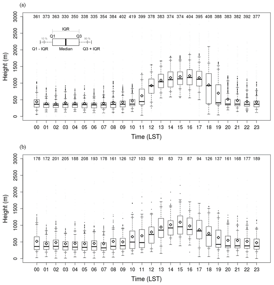
Figure 12 Box plots of hourly ABLHs estimated by ISABLE on (a) clear (cloud cover ≤ 30 %) and (b) cloudy (cloud cover ≥ 80 %) cases for the period from August 2016 to October 2018.

Figure 13 shows the diurnal variations of the ABLH for clear skies by season. The period mean maximum hourly ABLH was 1401 m at 15:00 LST in JJA (June, July, August; Fig. 13c) and the second-highest was 1257 m at 16:00 LST in SON (September, October, November; Fig. 13d). In DJF (December, January, February; Fig. 13a), the period mean maximum hourly ABLH was as low as 1093 m at 16:00 LST. This is consistent with the net radiation in an urban residential area in Seoul (Park et al., 2014). The minimum hourly ABLH showed the lowest value of 333 m at 02:00 LST in DJF and occurred at a relatively higher level of 470 m at 03:00 LST in JJA. The ABL during the nighttime in JJA is less thermodynamically stable than that in DJF, mainly due to anthropogenic heat release in urban areas.

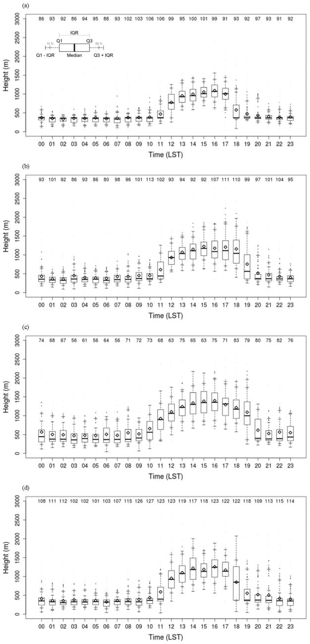
Figure 13 Box plots of hourly ABLHs for clear skies in (a) winter, (b) spring, (c) summer, and (d) autumn for the period from August 2016 to October 2018.

The hourly IQR is small before sunrise, increases with the evolution of ML, and decreases again after sunset in all seasons. Notably, it was the most considerable transition time near sunrise and sunset. The difference in IQR between the daytime and nighttime by season was evident in DJF, MAM, and SON but not in JJA. The ratio of IQR during nighttime to daytime in DJF was as low as 0.29 (02:00 LST, 92 m; 1600 LST, 311 m), while it was as high as 0.52 in JJA (02:00 LST, 295 m; 16:00 LST, 567 m). This implies that the estimated ABLHs are relatively dispersed both in daytime and nighttime in JJA.

ML and SBL growth and decline are directly affected by the sunrise and sunset periods. In the transition period, the uncertainty of the ABLH and the IQR increases. The IQR peaks occurred at 12:00 and 18:00 LST in DJF and at 11:00 and 19:00 LST in MAM. It can be seen that the evolution of ML occurred quickly, but the decline of ML or SBL evolution occurred slowly. The large IQR at 10:00 and 20:00 LST in JJA implied that the ML developed at the earliest time and declined at the latest time in summer. The large IQR at 12:00 and 18:00 LST in SON was due to the delayed sunrise and earlier sunset (Fig. 13d).

Figure 14 shows the seasonal distribution of the ABLH during the daytime (14:00 to 16:00 LST) and nighttime (03:00 to 05:00 LST). The mean ABLH during daytime was 1377, 1222, and 1184 m in JJA, SON, and MAM, respectively (Fig. 14a). The IQR in JJA (528 m) was larger than those in MAM (389 m) and SON (464 m). In DJF, the mean ABLH was the lowest (1049 m), and the IQR was the smallest (302 m). The mean ABLH at nighttime was the highest (474 m), and IQR was the largest (240 m) in JJA (Fig. 14b). The mean ABLH (IQR) was 413 m (151 m), 368 m (133 m), and 359 m (113 m) in MAM, SON, and DJF, respectively.

Figure 14 Box plot of seasonal ABLH during the (a) daytime (14:00 to 16:00 LST) and (b) nighttime (03:00 to 05:00 LST) for the period from August 2016 to October 2018.

Figure 15 shows diurnal variations of hourly mean net radiation and its 90th and 10th percentiles, as well as hourly mean ABLH estimated by ISABLE during the clear skies. Theoretically, the surface is heated from the time when net radiation becomes positive, and a ML evolves to balance the energy provided from the surface during the positive net radiation with the energy consumed to heat the overlying air volume. In reality, the ABL started to evolve from 3 h after the positive net radiation. The peak of net radiation occurred at 12:00 LST, while the peak of the ABLH occurred at about 16:00 LST. The ABLH declined rapidly at 1 to 2 h before the negative net radiation. The net radiation in MAM was similar to that in JJA and larger than that in SON, while the ABLH in MAM was similar to that in SON. The difference between the 10th and 90th percentiles of net radiation around 07:00 to 08:00 LST was more significant in MAM than in the other seasons. The differences around 12:00 to 13:00 LST in DJF are lower than in the other seasons. It implies that net radiation, as well as other minor factors, could fully explain the diurnal variation of the ABLH. The difference of net radiation at the same time in the same season could be mainly due to cloud and partly due to moisture and air pollutants.

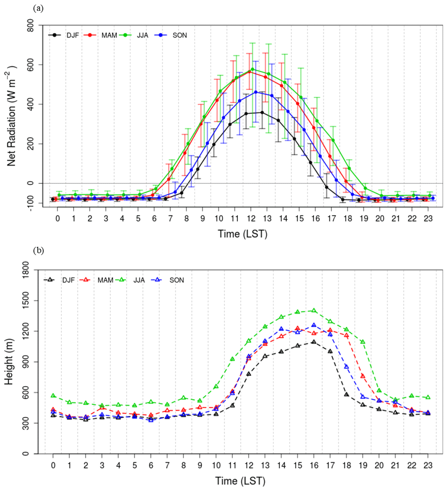
Figure 15 Seasonal mean diurnal variation of (a) net radiation with the 10th and 90th percentiles, and (b) ABLH estimated by ISABLE from August 2016 to October 2018.

6 Summary and discussion

The ISABLE algorithm developed in this study integrated the conventional ABLH estimation methodologies to produce optimal ABLH and applied statistical post-processing techniques to improve accuracy. A maximum of five ABLHs were estimated every 10 min using the ceilometer backscattering coefficient for each methodology (i.e., time-variance method, gradient method, wavelet covariance transform method, and clustering analysis method). The determined ABLHs were divided into five maximum clusters via the k-means cluster analysis method, and the ABLH was finally determined as the average of the members of the clusters satisfying the statistical conditions. The nocturnal SBLH was estimated using a potential temperature profile from a microwave radiometer. The SBLH was determined using the CLR method proposed in this study, which uses the threshold of the environmental lapse rate of potential temperature over the day. The ABLHs estimated by the ceilometer were post-processed in three steps (i.e., SNR threshold, instrument-related near-range artifact, and isolated ABLHs) to remove unreasonable values. The lowest altitude among the ABLH and the nocturnal SBLH was finally determined as an optimized ISABLE ABLH.

From 2015 to 2018, ABLH levels were determined using the ISABLE algorithm (ISABLE_ABLH) at 10 min intervals and were compared with and verified against the ABLH estimated by radiosonde observations (RS_ABLH) at Jungnang Station in Seoul city, Korea. The Ri_b was calculated using the vertical profile of the potential temperature and wind obtained by RS to estimate the ABLH during the entire sounding. The nocturnal SBLH was determined by the vertical temperature profile with the use of the SBI method at nighttime. The performance of ISABLE was verified by comparing the ISABLE_ABLH and ABLH estimated from each methodology with RS_ABLH. It was determined that the correlation coefficient between ISABLE_ABLH and RS_ABLH was the highest (R=0.72), as compared to other methodologies. The MB and RMSE showed the smallest values (−34 and 322 m), implying the best performance. Furthermore, the ISABLE algorithm was verified through the separation of the data into four time zones: i.e., daytime (12:00 to 17:00 LST), nighttime (23:00 to 05:00 LST), sunrise transition time (06:00 to 11:00 LST), and sunset transition time (18:00 to 22:00 LST). As a result, the correlation coefficient, MB, and RMSE between ISABLE_ABLH and RS_ABLH exhibited the best performance at 0.86, −3, and 236 m during daytime, respectively. Generally, the performance of ISABLE was found to be superior to the other four conventional methods, with some exceptions, especially in sunrise/sunset periods.

On the other hand, the ISABLE performance at nighttime was not as good as that in the other four conventional methods. It seems to be the difference in SBLH estimation between the RS and MWR, and further analyses on the difference are required. The presence of a RL and cloud layer caused large deviations by instruments and methodologies, thereby resulting in somewhat lower performance. The performances for all methodologies on clear skies were better than those on cloudy skies.

The diurnal variation of ISABLE_ABLH was also analyzed for the period from August 2016 to October 2018. ABLH began to grow from 09:00 to 11:00 LST after sunrise, reached a maximum at 15:00 to 16:00 LST, and declined at 18:00 to 20:00 LST. If the SBL was detected from the vertical profile of temperature at nighttime, the SBLH was estimated using the CLR method. Sometimes the top of the RL or cloud layer was determined as the ABLH; thus, the IQR of the ABLH increased.

The IQR of the ABLH was large during the daytime and small during the nighttime, and the deviations of the ABLH in both daytime and nighttime were more significant on clear days. Maximum hourly ABLH occurred in spring and summer, while minimum hourly ABLH occurred in winter. The IQR differences between the daytime and nighttime showed a large value in winter, spring, and autumn and a small value in summer. The differences showed two maxima at 10:00 and 18:00 LST in winter and at 09:00 and 20:00 LST in summer. The diurnal variation of net radiation was closely related to that of the ABLH, and further analyses on the peak time and energy balance are needed.

Most conventional methodologies have been verified for daytime clear skies over several days, while this study tried to attempt to include cloudy as well as complex conditions using the available data set during the 4 years. Poor performance was mainly due to multiple factors, such as strong backscattering signals in the RL, presence of clouds, and weak backscattering signals. Overall, the performance of ISABLE_ABLH was found to be better than that of the conventional methods. There were 28 cases with a difference between the RS-ABLH and the ABLH for each methodology exceeding 1000 m. Among them, 20 cases showed strong backscattering coefficients in RL at nighttime; thus, the ABLH was estimated as the corresponding altitude, especially using the GM and WAV2 methods. The remaining eight cases occurred during the daytime, six cases occurred in the presence of clouds, and two cases occurred in apparently clear skies with very weak backscattering signals. The foregoing cases often appear in a real atmosphere; however, it is difficult to estimate the consistent ABLHs under the aforementioned atmospheric conditions. In this study, as the ABLH was estimated using as much data as possible, regardless of time or atmospheric conditions, their performances seemed to be somewhat lower. When convection is robust during the daytime, the atmospheric structure is relatively homogeneous below the ABLH, and the results of ABLH determinations via different methodologies are similar. On the other hand, if the atmospheric structure is complicated, such as the presence of nocturnal SBL, RL, and daytime clouds, the ABLH may be different from those of the methodologies, and the criteria for determining true ABLH remain with researchers. In addition, in the estimation of the SBLH by the CLR method using the MWR, further studies are needed due to the lack of verification cases.

Although the ISABLE-estimated ABLH exhibited better performance than those estimated by the earlier conventional methodologies, there are still many limitations. In particular, ABLHs estimated from the ceilometer in the lower layer are not reliable due to near-range artifacts, especially under intense solar radiation. ABLHs at higher levels at nighttime could be supplemented by the temperature profile obtained by the MWR. ABLHs are challenging in terms of estimating under cloudy sky or precipitation, severe fog, and smog events. Since the ISABLE algorithm is in the early stage of development, it did not address all the known issues yet, such as precipitation, lofted aerosol layer, and too clean (little aerosol) a condition. These limitations and drawbacks should be overcome by combining enough observation data, instrumental advances, and the corresponding improvements of ISABLE.