Ensemble-based satellite-derived carbon dioxide and methane column-averaged dry-air mole fraction data sets (2003–2018) for carbon and climate applications

Satellite retrievals of column-averaged dry-air mole fractions of carbon dioxide (CO₂) and methane (CH₄), denoted XCO₂ and XCH₄, respectively, have been used in recent years to obtain information on natural and anthropogenic sources and sinks and for other applications such as comparisons with climate models. Here we present new data sets based on merging several individual satellite data products in order to generate consistent long-term climate data records (CDRs) of these two Essential Climate Variables (ECVs). These ECV CDRs, which cover the time period 2003–2018, have been generated using an ensemble of data products from the satellite sensors SCIAMACHY/ENVISAT and TANSO-FTS/GOSAT and (for XCO₂) for the first time also including data from the Orbiting Carbon Observatory 2 (OCO-2) satellite. Two types of products have been generated: (i) Level 2 (L2) products generated with the latest version of the ensemble median algorithm (EMMA) and (ii) Level 3 (L3) products obtained by gridding the corresponding L2 EMMA products to obtain a monthly $\mathrm{5}{}^{\circ }\times \mathrm{5}{}^{\circ }$ data product in Obs4MIPs (Observations for Model Intercomparisons Project) format. The L2 products consist of daily NetCDF (Network Common Data Form) files, which contain in addition to the main parameters, i.e., XCO₂ or XCH₄, corresponding uncertainty estimates for random and potential systematic uncertainties and the averaging kernel for each single (quality-filtered) satellite observation. We describe the algorithms used to generate these data products and present quality assessment results based on comparisons with Total Carbon Column Observing Network (TCCON) ground-based retrievals. We found that the XCO₂ Level 2 data set at the TCCON validation sites can be characterized by the following figures of merit (the corresponding values for the Level 3 product are listed in brackets) – single-observation random error (1σ): 1.29 ppm (monthly: 1.18 ppm); global bias: 0.20 ppm (0.18 ppm); and spatiotemporal bias or relative accuracy (1σ): 0.66 ppm (0.70 ppm). The corresponding values for the XCH₄ products are single-observation random error (1σ): 17.4 ppb (monthly: 8.7 ppb); global bias: −2.0 ppb (−2.9 ppb); and spatiotemporal bias (1σ): 5.0 ppb (4.9 ppb). It has also been found that the data products exhibit very good long-term stability as no significant long-term bias trend has been identified. The new data sets have also been used to derive annual XCO₂ and XCH₄ growth rates, which are in reasonable to good agreement with growth rates from the National Oceanic and Atmospheric Administration (NOAA) based on marine surface observations. The presented ECV data sets are available (from early 2020 onwards) via the Climate Data Store (CDS, https://cds.climate.copernicus.eu/, last access: 10 January 2020) of the Copernicus Climate Change Service (C3S, https://climate.copernicus.eu/, last access: 10 January 2020).

1 Introduction

Carbon dioxide (CO₂) and methane (CH₄) are important greenhouse gases and increasing atmospheric concentrations result in global warming with adverse consequences such as sea level rise (IPCC, 2013). Because of their importance for climate, these gases have been classified as Essential Climate Variables (ECVs) by the Global Climate Observing System (GCOS) (GCOS-154, 2010; GCOS-200, 2016). The generation of XCO₂ and XCH₄ satellite-derived ECV data products meeting GCOS requirements using European satellite retrieval algorithms started in 2010 in the framework of the GHG-CCI project (http://www.esa-ghg-cci.org/, last access: 10 January 2020) of the European Space Agency's (ESA) Climate Change Initiative (CCI) (Hollmann et al., 2013). Since the end of 2016, this activity continues operationally via the Copernicus Climate Change Service (C3S, https://climate.copernicus.eu/, last access: 10 January 2020), and the corresponding CO₂ and CH₄ data products are available via the Copernicus Climate Data Store (CDS, https://cds.climate.copernicus.eu/, last access: 10 January 2020). These ECV data products have been used for a range of applications such as improving our knowledge of CO₂ and/or CH₄ surface fluxes (e.g., Alexe et al., 2015; Basu et al., 2013; Buchwitz et al., 2017a; Chevallier et al., 2014, 2015; Ganesan et al., 2017; Gaubert et al., 2019; Houweling et al., 2015; Liu et al., 2017; Maasakkers et al., 2019; Miller et al., 2019; Reuter et al., 2014a, b, 2019a; Sheng et al., 2018; Schneising et al., 2014b; Turner et al., 2015, 2019), comparison with climate and other models (e.g., Hayman et al., 2014; Lauer et al., 2017; Schneising et al., 2014a), and for other applications such as computation of CO₂ growth rates (e.g., Buchwitz et al., 2018), as well as to better understand changes in the amplitude of the CO₂ seasonal cycle (e.g., Yin et al., 2018).

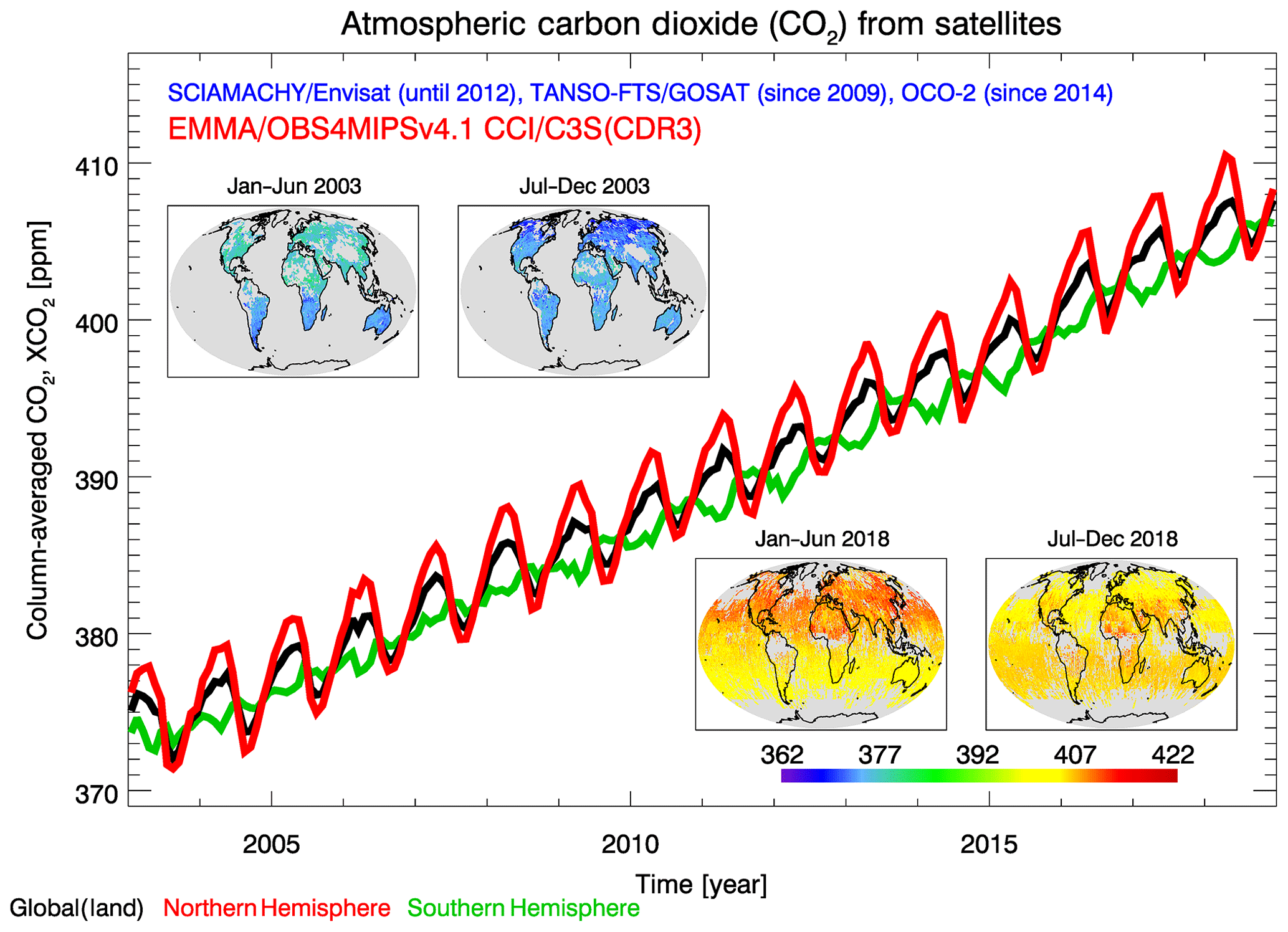
Figure 1 Overview of the presented XCO₂ data set. Shown are time series over land for three latitude bands (global, black line; Northern Hemisphere, red; Southern Hemisphere, green) and global maps (half-yearly averages at $\mathrm{1}{}^{\circ }\times \mathrm{1}{}^{\circ }$ obtained by gridding (averaging) the merged Level 2, i.e., EMMA, product). See Sect. 4 for a detailed discussion.

Figure 2 As Fig. 1 but for XCH₄.

The C3S satellite greenhouse gas (GHG) data set consists of single-sensor satellite data products and of merged (i.e., combined multi-sensor, multi-algorithm) data products. Here we present the latest version, version 4.1, of the merged Level 2 (L2) and merged Level 3 (L3) XCO₂ and XCH₄ data products, which cover the time period 2003–2018. The L2 products (XCO2_EMMA and XCH4_EMMA) have been compiled with the ensemble median algorithm (EMMA) originally proposed by Reuter et al. (2013) and recent modifications, which are described in Sect. 3.1. These products contain detailed information for each single observation (i.e., footprint or ground pixel) including time, latitude and longitude, the main parameter (i.e., XCO₂ or XCH₄), its stochastic uncertainty (e.g., due to instrument noise), an estimate of potential systematic uncertainties (e.g., due to spatial or temporal bias patterns), and its averaging kernel and corresponding a priori profile. The L3 products (XCO2_OBS4MIPS and XCH4_OBS4MIPS) are gridded products at monthly time and $\mathrm{5}{}^{\circ }\times \mathrm{5}{}^{\circ }$ spatial resolution in Obs4MIPs (Observations for Model Intercomparisons Project, https://www.earthsystemcog.org/projects/obs4mips/, last access: 10 January 2020) format.

Figure 1 provides an overview of the resulting merged XCO₂ data product in terms of time series for three latitude bands and global maps and the similarly structured Fig. 2 shows the XCH₄ product. As can be seen, XCO₂ and XCH₄ are both increasing with time and exhibit seasonal fluctuations and spatial variations. The spatiotemporal characteristics of the merged data – e.g., the spatial sampling – reflect the characteristics of the underlying individual sensor satellite data (described in the data section, Sect. 2). Figures 1 and 2 are discussed in detail in the results section, Sect. 4. How these data products have been generated is described in the methods section, Sect. 3. A summary and conclusions are given in Sect. 5.

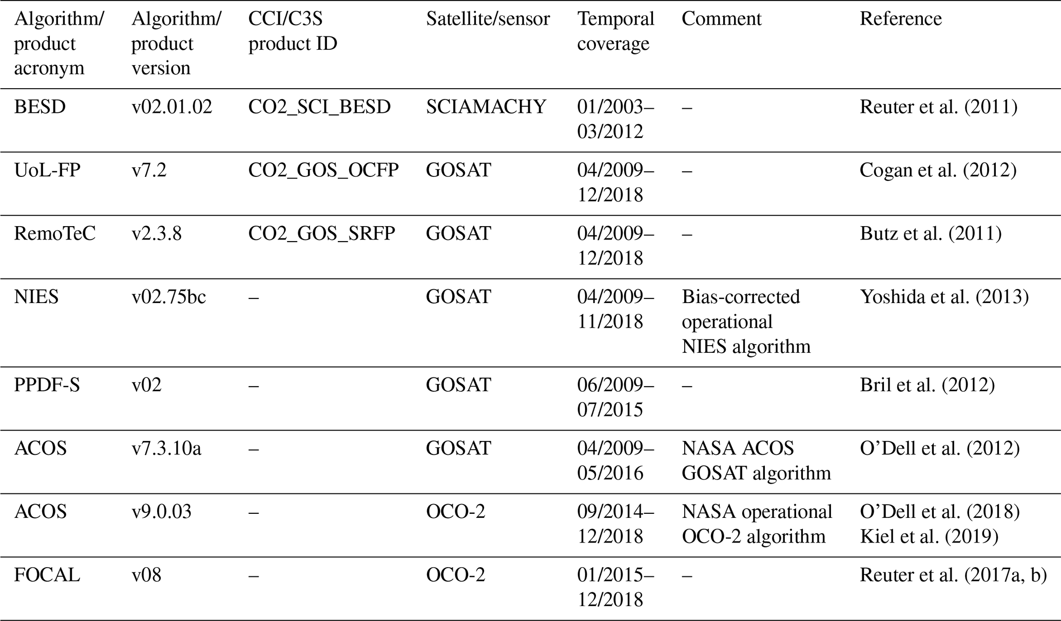
Table 1 Satellite XCO₂ Level 2 (L2) data products used as input for the generation of the merged L2 and L3 XCO₂ version 4.1 data products. For products which have been generated in the framework of the CCI and C3S projects the corresponding product ID is listed (the other products are external products, which have been obtained from the corresponding websites; see Acknowledgements). Temporal coverage indicates the time coverage of the input data sets.

2 Data

In this section, we present an overview about the input data used to generate and validate the new XCO₂ and XCH₄ data products.

2.1 Satellite data

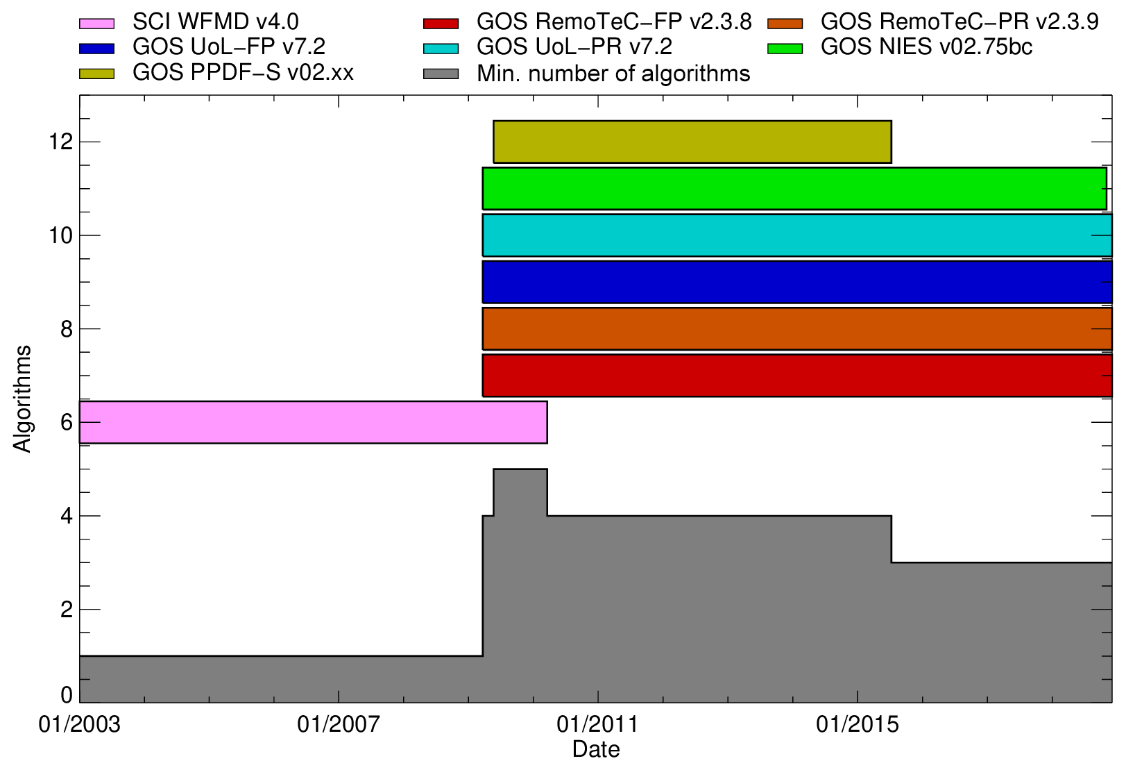
The input satellite data used to generate the merged satellite data products are individual satellite sensor Level 2 (L2) data products. Table 1 provides an overview about the satellite XCO₂ input data sets. As can be seen, in total eight XCO₂ L2 data products have been used to generate the merged L2 and Level 3 (L3) XCO₂ data products, each corresponding to a different combination of satellite sensor and retrieval algorithm. An overview about the time coverage of these input data products is presented in Fig. 3. As can be seen, the time period 2003 to March 2009 is only covered by one XCO₂ product, namely XCO₂ retrieved with the Bremen Optimal Estimation DOAS (BESD) algorithm (Reuter et al., 2010, 2011) from the SCIAMACHY/ENVISAT (Bovensmann et al., 1999) instrument. A second SCIAMACHY XCO₂ data product is available, which has been retrieved with the Weighting Function Modified Differential Optical Absorption Spectroscopy (WFM-DOAS or WFMD) algorithm (Schneising et al., 2011), but this product is not used because the merging algorithm EMMA (Reuter et al., 2013, described in Sect. 3.1) requires one or more than two input data products (because the median of a set of elements is, according to our definition which avoids averaging, not defined for two elements). Therefore, one of the two products had to be selected, and the choice was the BESD product for XCO₂ because of somewhat higher data quality compared to the WFMD product (Buchwitz et al., 2017b) (note however that the WFMD product has the advantage of containing a larger number of observations). As can be seen from Table 1 and Fig. 3, several GOSAT input products have been used from April 2009 onwards and two OCO-2 XCO₂ products from September 2014 and May 2015 onwards. Note that additional algorithms/data products are available but have not been used as input, for example the GOSAT BESD XCO₂ product (Heymann et al., 2015) and the OCO-2 RemoTeC XCO₂ product (Wu et al., 2018). These or other additional products may be added in future versions of the merged XCO₂ products. Note also that we always use the bias-corrected version of a data product, if available (some product files contain bias-corrected and uncorrected values).

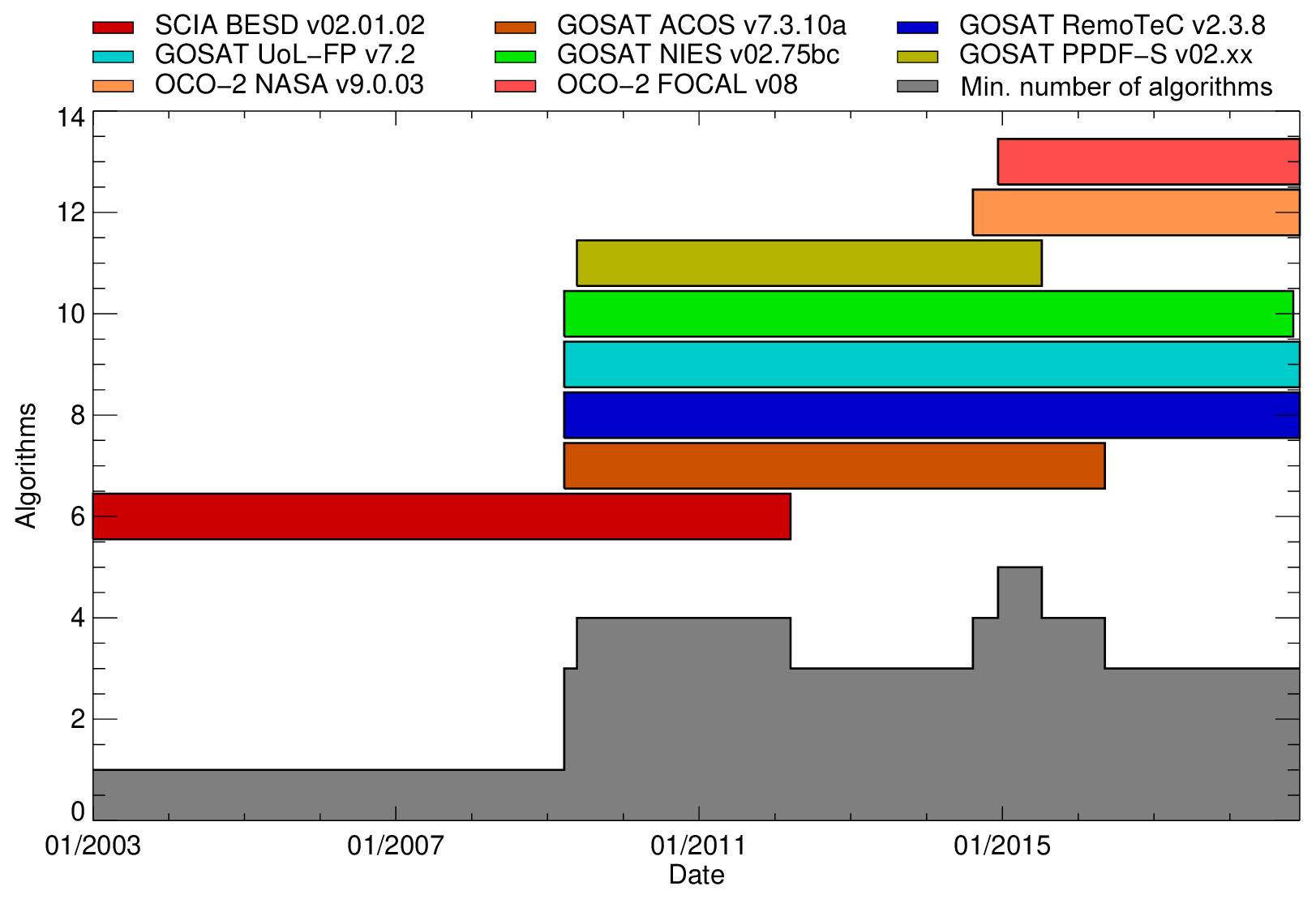
Figure 3 Individual satellite sensor XCO₂ data products contributing to the merged XCO₂ data products (see Table 1 for details). The required minimum number of contributing products is shown by the grey area.

All listed satellites perform nadir (down-looking) and glint observations and provide radiance spectra covering the relevant CO₂ and CH₄ absorption bands located in the shortwave infrared (SWIR) part of the electromagnetic spectrum (around 1.6 and 2 µm) and also cover the O₂ A-band spectral region in the near-infrared (NIR, around 0.76 µm). All individual sensor input L2 data products have been generated using retrieval algorithms based on minimizing the difference between a modeled radiance spectrum and the observed spectrum by modifying so-called state vector elements (for details we refer to the references listed in Table 1; for additional information see also the Algorithm Theoretical Basis Documents (ATBDs); Buchwitz et al., 2019b, and Reuter et al., 2019b). The exact definition of the state vector depends on the algorithm, but the general approach is based on the optimal estimation (Rodgers, 2000) formalism or similar approaches (see references in Table 1). Among the state vector elements is a representation of the CO₂ vertical profile but also other parameters to consider interfering gases (e.g., water vapor), surface reflection, atmospheric scattering, and other effects and parameters, which have an impact on the (interpretation of the) measured radiance spectrum.

Table 2 As Table 1 but for XCH₄.

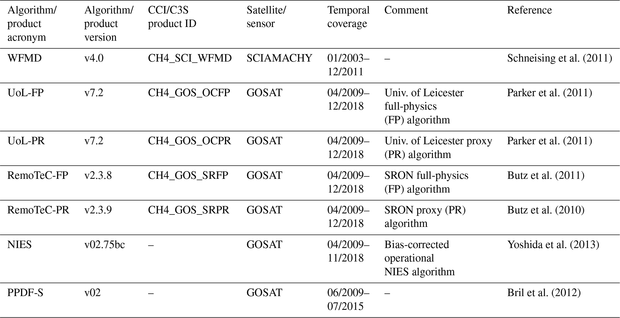
Table 3 TCCON sites used for the validation of the XCO₂ and XCH₄ satellite-derived data products.

Table 2 and Fig. 4 provide an overview about the satellite XCH₄ L2 input data sets. As for XCO₂, the time period 2003 to March 2009 is only covered by one SCIAMACHY data product. From April 2009 onwards several GOSAT XCH₄ products are available (see Table 2) and have been used to generate the merged XCH₄ data L2 and L3 data products. For future updates it is also planned to include XCH₄ from the Sentinel-5 Precursor (S5P) satellite (Veefkind et al., 2012), but S5P XCH₄ (Hu et al., 2018; Schneising et al., 2019) has not yet been included as the time period covered by these products is currently quite short (less than 2 years). However, we aim to include S5P XCH₄ for one of the next updates of the merged methane products.

Figure 4 As Fig. 3 but XCH₄. For details on each product see Table 2.

2.2 Ground-based data

The satellite data products have been validated by comparison with the XCO₂ and XCH₄ data products of the TCCON (Wunch et al., 2011). TCCON is a network of ground-based Fourier transform spectrometers (FTSs) recording direct solar spectra in the NIR/SWIR spectral region. From these spectra, accurate and precise column-averaged abundances of CO₂, CH₄, and a number of other species are retrieved. The TCCON data products (version GGG2014) have been obtained via the TCCON data archive (https://tccondata.org/, last access: 15 July 2019). An overview about the used TCCON sites is presented in Table 3.

In Sect. 4.3, we present annual XCO₂ and XCH₄ growth rates, which have been derived from the new XCO₂ and XCH₄ OBS4MIPS data products using the method described in Buchwitz et al. (2018). These growth rates are compared with growth rates derived from marine surface CO₂ and CH₄ observations, which have been obtained from the National Oceanic and Atmospheric Administration (NOAA) (for details including links and last access see Acknowledgements).

3 Methods

3.1 Merging algorithm EMMA

In order to generate the merged L2 products, the ensemble median algorithm is used, which is described in detail in Reuter et al. (2013). Therefore, we limit the description given here to a short overview of the latest version of the EMMA algorithm. To be specific, we initially describe the EMMA XCO₂ algorithm and explain differences relevant for XCH₄ at the end of this subsection.

The EMMA XCO₂ data product consists of selected individual L2 soundings from the available individual sensor L2 input products (listed in Table 1). The EMMA L2 product is based on selecting the best soundings (i.e., single ground pixel observations) from the ensemble of individual sensor L2 products. Sounding selection is based on monthly time and $\mathrm{10}{}^{\circ }\times \mathrm{10}{}^{\circ }$ spatial intervals. To decide which individual product is selected for a given month and given grid cell, all input products are first gridded (monthly, $\mathrm{10}{}^{\circ }\times \mathrm{10}{}^{\circ }$) to consider the fact that the spatiotemporal sampling is different for each individual product (due to different satellite sensors and algorithm-dependent quality-filtering strategies). The selected product is the median in terms of average XCO₂ per month and grid cell (note that in case of an even number of products the product which is closest to the mean is selected). The median is used primarily to remove potential outliers. The advantage of the median is also (in contrast to, for example, the arithmetic mean) that no averaging or other modifications to the input data are required. In order for a grid cell to be assigned a valid value, the following criterion has to be fulfilled: a minimum number of data products having a standard error of the mean (SEOM) of less than 1 ppm has to be available (see grey area in Fig. 3). SEOM is defined by $\frac{\mathrm{1}}{n}\sqrt{{\sum }_i{\mathit{\sigma }}_i^{\mathrm{2}}}$, with σ_i being the (scaled; see below) XCO₂ uncertainty of the ith out of n soundings.

This means that EMMA selects for each month and each $\mathrm{10}{}^{\circ }\times \mathrm{10}{}^{\circ }$ grid cell exactly one product of the available individual L2 input products and then transfers all relevant information (i.e., XCO₂ and its uncertainty, related averaging kernels and a priori profile, etc.) from the selected original L2 file into the corresponding daily EMMA L2 product file. This ensures that most of the original information from the selected individual product is also contained in the merged product.

However, some modifications are applied. In order to remove (or at least to minimize) the impact of different a priori assumptions, all products are converted to common a priori CO₂ vertical profiles (see Reuter et al., 2013, for details). The new a priori profiles are obtained from the simple empirical CO₂ model (SECM, Reuter et al., 2012). SECM is essentially an empirically found function with parameters optimized using a CO₂ model (CT2017; see below). The SECM model used here is referred to as SECM2018 and is an update of the SECM model described in Reuter et al. (2012). The main difference is that SECM2018 is using a recent version of NOAA's assimilation system CarbonTracker (Peters et al., 2007, with updates documented at: http://carbontracker.noaa.gov/, last access: 10 January 2020), namely CT2017.

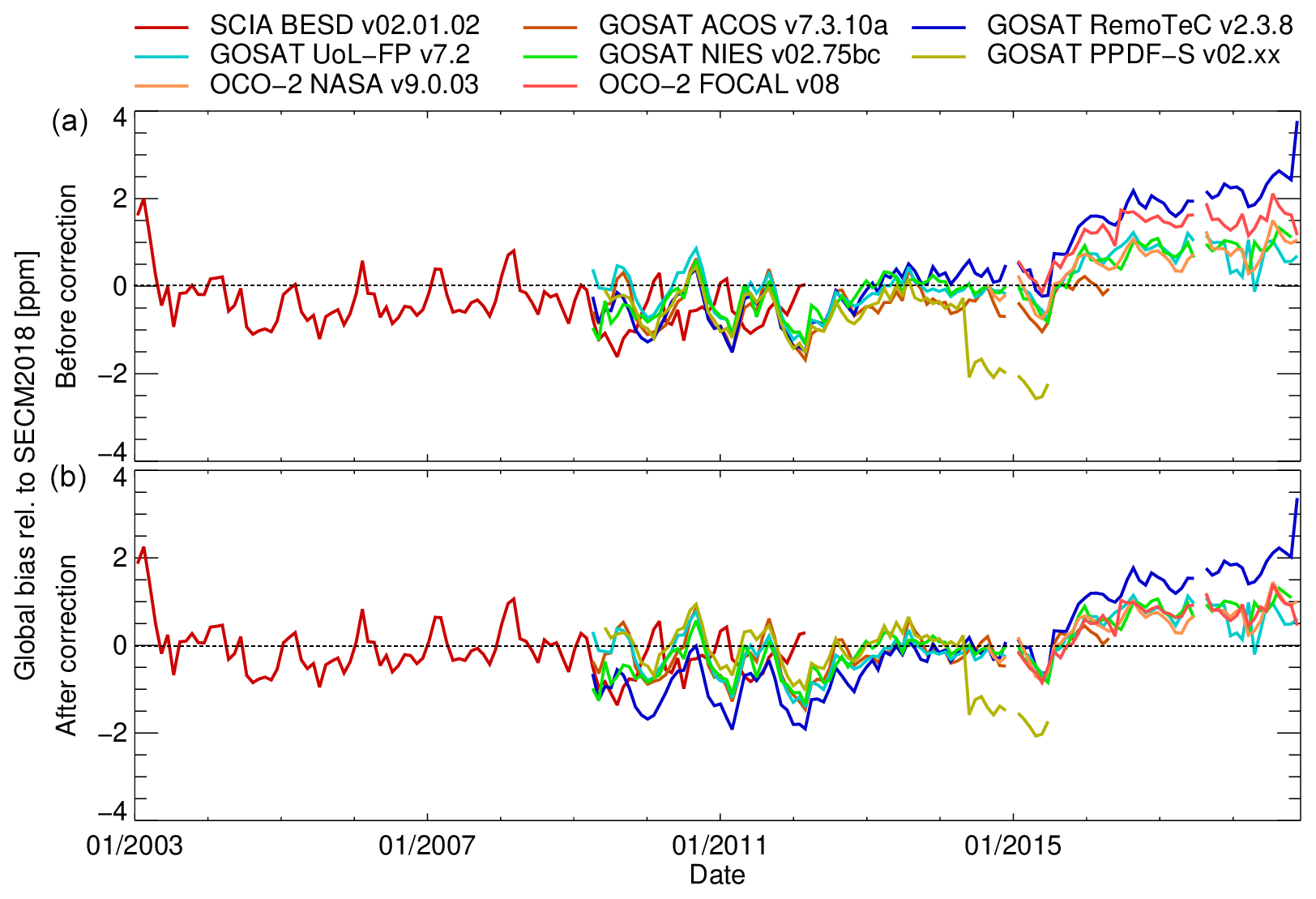
Figure 5 Global bias correction as applied by EMMA to the individual satellite XCO₂ input data products. Panel (a) shows the difference relative to the SECM2018 model (computed as satellite – model) before the correction and (b) shows the difference after correction.

SECM2018 is also used to correct for potential offsets between the individual data products by adding or subtracting a global offset (i.e., by using one constant offset value for each individual product applied globally and for the full time series). Time series of the individual data products before and after offset correction are shown in Fig. 5. Note that in Fig. 5 all data are relative to SECM2018, which is a very simple CO₂ model, and therefore all variations and trends seen in Fig. 5 are at least to some extent model errors. As can be seen from Fig. 5, the correction brings the individual data sets typically closer together without changing any of their other characteristics (e.g., their time dependence). But as can also be seen from Fig. 5, better agreement is only achieved on average, not necessarily for all products during the entire time period. For example, the GOSAT RemoTeC product (blue curve) during 2009–2012 exhibits a somewhat larger difference after the offset correction. The approximately 2 ppm (0.5 %) spike at the beginning of the time series is likely due to a positive bias of the underlying BESD data product, which has not been corrected due to the lack of reference data in this time period (see also the discussion of this aspect in Buchwitz et al., 2018). An obvious issue is also the approximately 1.5 ppm (0.4 %) discontinuity in the first half of 2014 of the PPDF-S (photon path length probability density function/simultaneous) product (light-green curve). Depending on application, this may be an issue when this product is used stand-alone, but this is not a problem for EMMA as EMMA identifies and ignores outliers.

Another modification applied to the individual L2 input products is a potential scaling of their reported uncertainty for the individual L2 soundings. The scaling factor has been chosen such that on average the uncertainty of the reported error is consistent with the standard deviation of satellite minus ground-based validation data differences (see Sect. 4.1 for the validation of the reported uncertainties via the uncertainty ratio).

In order to avoid that an individual input product, which has much more observations than the other products (such as OCO-2 compared to GOSAT), entirely dominates the EMMA product, a method has been implemented to prevent overweighting the contributions from individual L2 input data products. The method is based on limiting the number of L2 data points. For each grid cell and month, we perform the following steps: first, we compute SEOM for each algorithm. From these values, we compute the 25th percentile and divide it by $\sqrt{\mathrm{2}}$. The result is used as the minimum SEOM threshold. If SEOM of an individual algorithm is smaller than this threshold, a subset of soundings is randomly chosen such that SEOM becomes just larger than the threshold. If, for example, all σ_i are 1 ppm, then SEOM simply becomes $\mathrm{1}/\sqrt{n}$. If in this case, for example, data from four algorithms were available with n₁=60, n₂=80, n₃=100, and n₄=1000, the SEOM threshold would become $\mathrm{1}/\sqrt{\mathrm{2}{n}_{\mathrm{3}}}$, which would effectively limit the number of soundings of the fourth algorithm to 200 (chosen randomly).

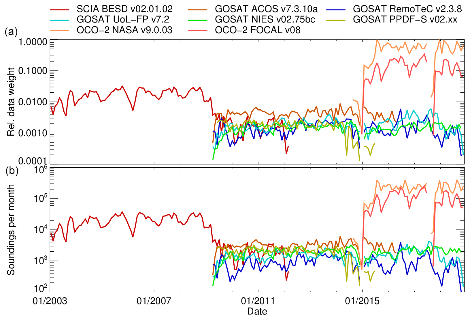
Figure 6 Relative data weight (a) and soundings per month (a) of the individual satellite XCO₂ data products contributing to the EMMA XCO₂ data product.

In addition to the L2 information of the selected data products, EMMA stores the following diagnostic information for each selected sounding: identifier for the selected L2 algorithm and inter-algorithm spread (IAS) within the grid box of the sounding. Within each grid box, IAS is defined as the algorithm-to-algorithm standard deviation of the grid box averages.

By how much each individual satellite XCO₂ data product contributes to the EMMA XCO₂ product is shown in Fig. 6. Figure 6a shows the relative data weight (RDW), and Fig. 6b shows the number of soundings per month. How the RDW is defined is explained in detail in Reuter et al. (2013). In short, the RDW is defined as the relative number of soundings weighted with the corresponding (square of the inverse) uncertainty. RDW is high if a (relatively) large number of soundings contribute to the EMMA product and if these soundings have (relatively) low uncertainty compared to the other contributing products. The RDW of a product is a measure of how much information on XCO₂ this product contributes to the EMMA product relative to the other contributing products. As can be seen from Fig. 6, the SCIAMACHY BESD product is the only product until early 2009, when the GOSAT time series starts. As can also be seen, OCO-2 dominates in terms of RDW and number of soundings from 2015 onwards. This is because OCO-2 provides much more data with typically better uncertainty compared to the other (GOSAT) product.

Figure 7 As Fig. 5 but for XCH₄ and using methane model SC4C2018.

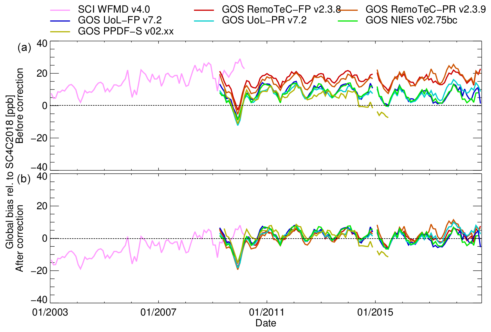
The EMMA L2 XCH₄ product has been generated similarly to the EMMA L2 XCO₂ product, i.e., using essentially the same method as described above. A difference is that the offset correction has been done with a CH₄ model instead of SECM2018. This model is the simple CH₄ climatological model (SC4C), and we use the year 2018 update referred to as SC4C2018 in the following. The SC4C2018 model is similar to SECM2018 but for XCH₄. It is a model-based CH₄ climatology adjusted for the annual growth rate (note that this model has also been used as the climatological training and a calibration data set as described in Schneising et al., 2019). The EMMA algorithm SEOM limit controlling the minimum number of data points per grid box, month, and algorithm has been set to 12 ppb for XCH₄. The impact of the offset correction for merging the XCH₄ products is shown in Fig. 7. Note that in Fig. 7 all data are relative to SC4C2018, which is a very simple CH₄ model, and therefore all variations and trends seen in Fig. 7 are at least to some extent model errors. As for CO₂ (Fig. 5) the offset correction typically brings the various XCH₄ products closer together but does not change any of their other characteristics. The PPDF-S product suffers from a discontinuity (of 8 ppb or 0.4 %) in the first half of 2014 (see above for a similar problem for PPDF-S XCO₂).

Figure 8 As Fig. 6 but for XCH₄.

Figure 8a shows the RDW, and Fig. 8b shows the number of soundings per month for all individual sensor XCH₄ products contributing to the XCH₄ EMMA product. Until early 2009, the SCIAMACHY WFMD product is the only product contributing to the EMMA product. Note that the RDW of the SCIAMACHY products drops at the end of 2005 (in contrast to the absolute number of soundings per month). The reason is the increase in the uncertainty of this product due to detector degradation (see, e.g., Schneising et al., 2011, for details). As can also be seen, the two GOSAT proxy (PR) products (i.e., CH4_GOS_OCPR and CH4_GOS_SRPR) dominate the XCH₄ EMMA product because they contain more soundings compared to the other (GOSAT) data products.

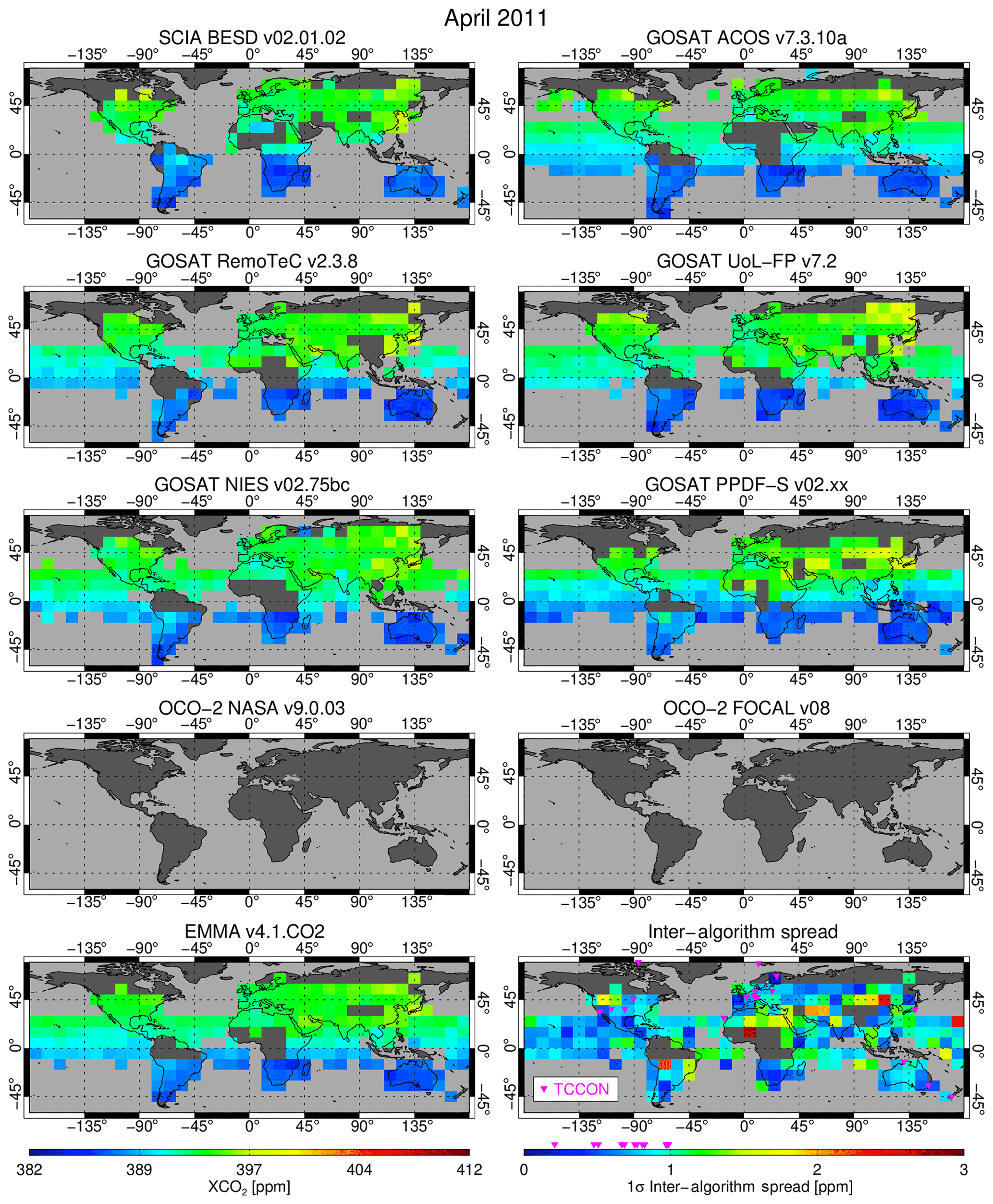
Figure 9 April 2011 XCO₂ at $\mathrm{10}{}^{\circ }\times \mathrm{10}{}^{\circ }$ spatial resolution showing (i) the individual sensor/algorithm input data sets (panels in rows 1–4; see Table 1 for details), (ii) EMMA XCO₂ (bottom left), and (iii) the inter-algorithm spread (IAS, 1σ) as computed by EMMA (bottom right; see main text for details). Also shown in the bottom-right panel are the locations of the TCCON sites (pink triangles) and the range of IAS values covered by them (see color bar). Note that the OCO-2 maps (row 4) are empty because this satellite was launched after April 2011 (see Fig. 10 for OCO-2 XCO₂).

3.2 Algorithm to generate the Level 3 OBS4MIPS products

The version 4.1 L3 XCO2_OBS4MIPS and XCH4_OBS4MIPS data products have been obtained by gridding (averaging) the version 4.1 L2, i.e., XCO2_EMMA and XCH4_EMMA, products using monthly time and $\mathrm{5}{}^{\circ }\times \mathrm{5}{}^{\circ }$ spatial resolution. The algorithm for the generation of the OBS4MIPS products is described in Reuter et al. (2019b). Therefore, we here provide only a short overview.

For each individual product, the gridding is based on computing an arithmetic, unweighted average of all soundings falling in a grid box.For each grid box, the standard error of the mean is computed using the uncertainties contained in the corresponding EMMA product files. In order to reduce noise at least two individual observations must be present and the resulting standard error of the mean must be less than 1.6 ppm for XCO₂ and less than 12 ppb for XCH₄.

Besides XCO₂ or XCH₄, the final L3 product also includes (per grid box and month) the number of soundings used for averaging; the average column-averaging kernel; the average a priori profile; the standard deviation of the averaged XCO₂ or XCH₄ values; and an estimate for the total uncertainty computed as the root sum square of two values, where one value is SEOM and the other value is IAS as computed by EMMA. For cases including only one algorithm, the second value is replaced by quadratically adding spatial and seasonal accuracy determined from the TCCON validation.

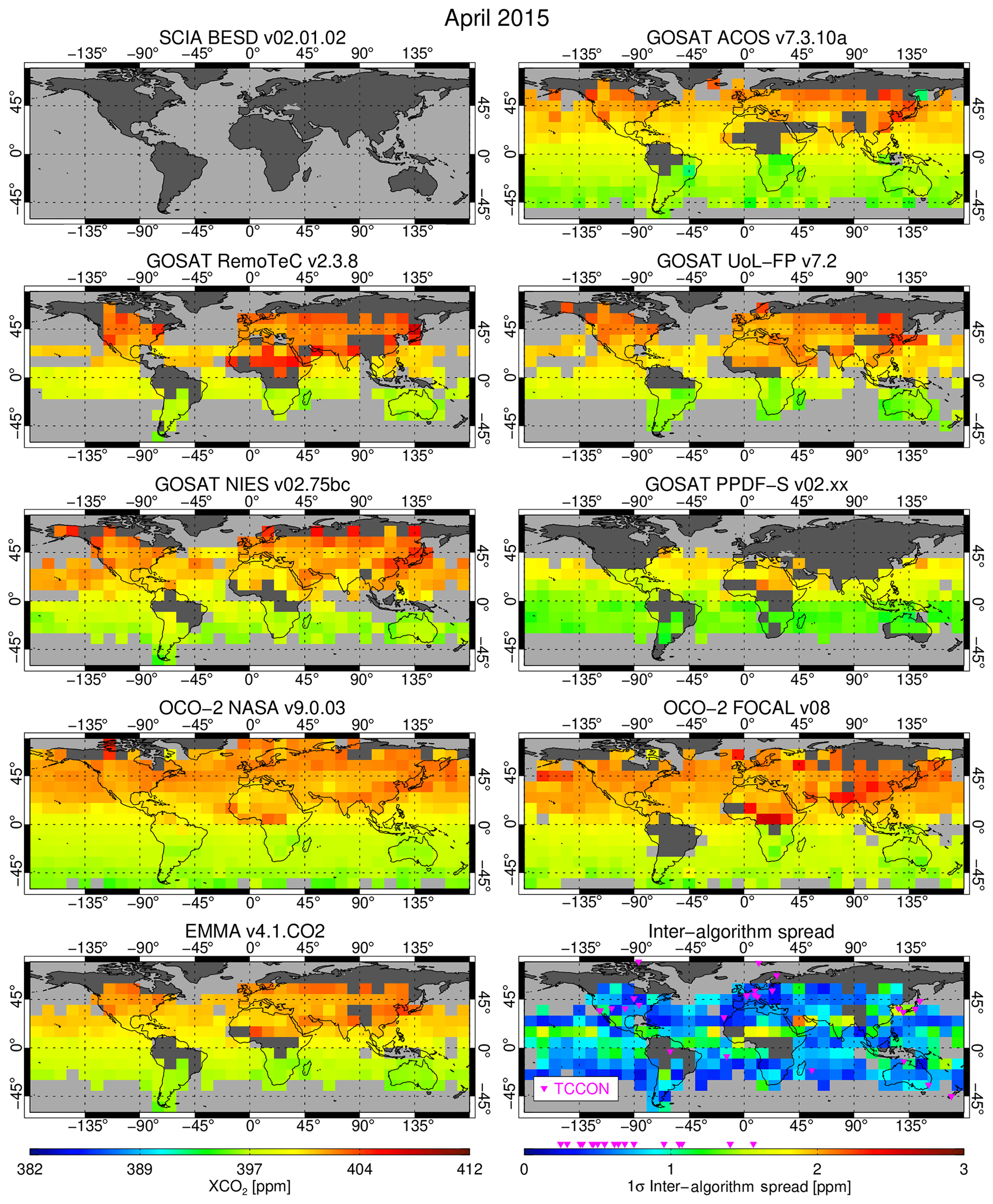
Figure 10 As Fig. 9 but for April 2015. Note that the SCIAMACHY/BESD map (top left) is empty because this product ended in April 2012 (see Fig. 9 for SCIAMACHY/BESD XCO₂).

3.3 Validation method

The validation of the merged satellite-derived XCO₂ and XCH₄ data products is based on comparisons with ground-based XCO₂ and XCH₄ TCCON observations (using version GGG2014). We present results from two somewhat different validation methods (the EMMA method, Reuter et al., 2013; and the QA/QC method, Buchwitz et al., 2017b; see below), which are similar to other validation methods used in recent years (e.g., Butz et al., 2010; Cogan et al., 2012; Dils et al., 2014; O'Dell et al., 2018; Parker et al., 2011). These methods differ with respect to details such as the chosen colocation criterion, whether the data are brought to a common a priori or not, and if yes which a priori has been used. In the following, we will highlight some of these details as relevant for the two validation methods used for this paper.

Both methods used for the validation of the L2 EMMA products are based on colocating each individual satellite XCO₂ (or XCH₄) observation with a corresponding value obtained from TCCON using predefined spatial and temporal colocation criteria (see below). The comparisons take into account different a priori assumptions regarding the vertical profiles of CO₂ (or CH₄) as used for the generation of the L2 input products by converting either the satellite data (QA/QC method) or the TCCON data (EMMA method) to a common a priori. This a priori correction is based on using the satellite averaging kernels and a priori profiles, which are contained (for each single observation) in the EMMA product files. The magnitude of the a priori correction (the explicit formula is shown as Eq. 3 in Dils et al., 2014) depends on the deviation (difference) of the averaging kernel from unity and on the difference of the a priori profiles. Because the averaging kernel profiles are typically close to unity (note that both satellite and the TCCON retrievals correspond to cloud-free conditions) and because the a priori profiles are not totally unrealistic, the a priori correction is typically very small (approximately 0.1 ppm for XCO₂ and 1 ppb for XCH₄).

Table 4 Overview validation results at TCCON sites for data product XCO2_EMMA (version 4.1).

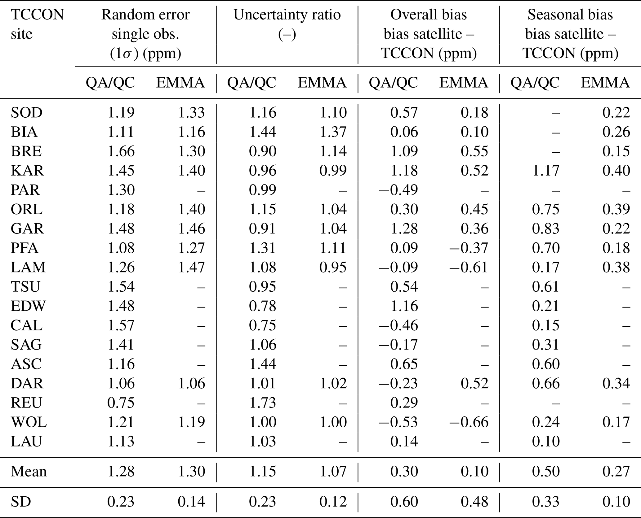
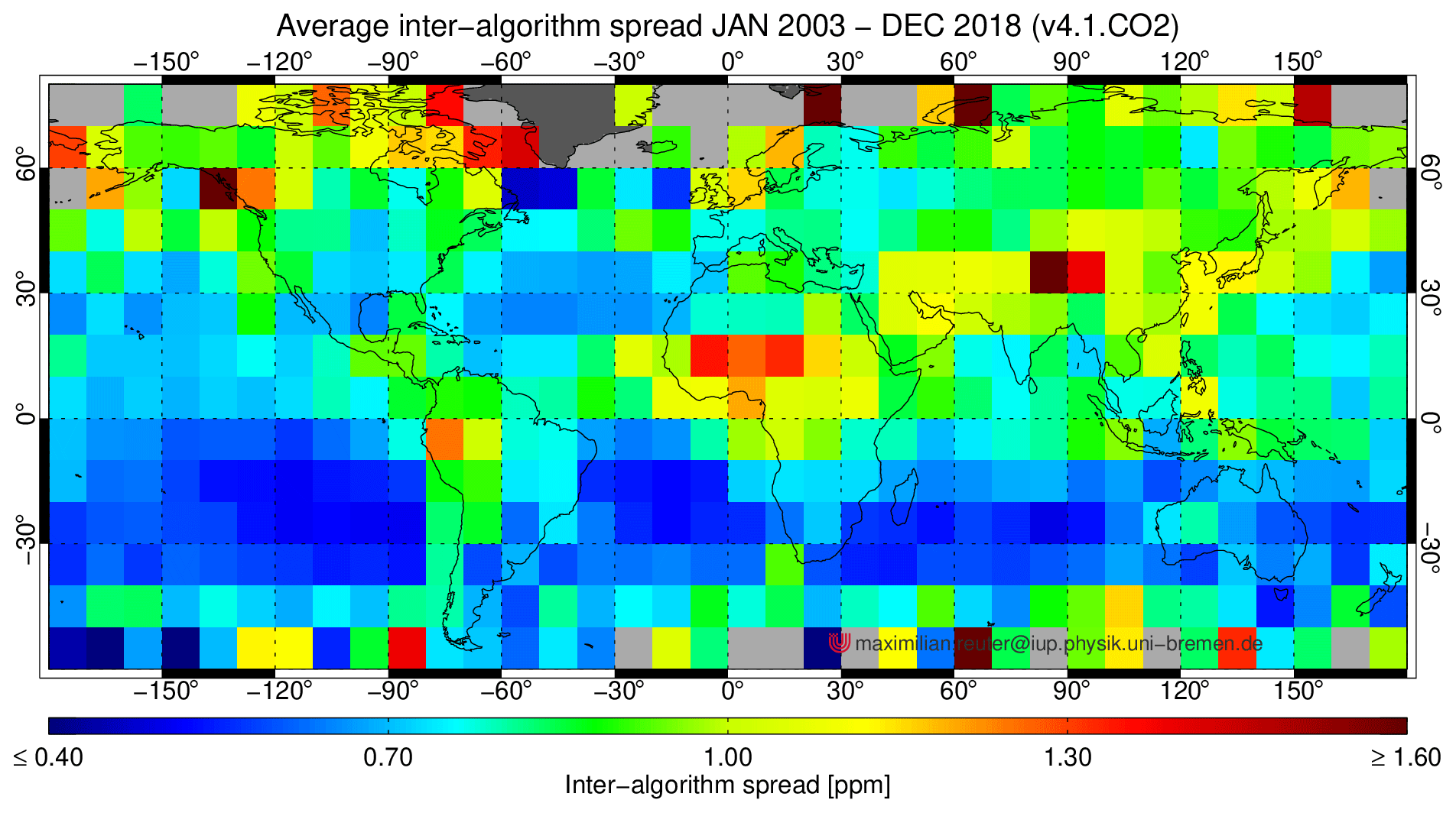
Figure 11 Average XCO₂ inter-algorithm spread (1σ) during 2003–2018. As can be seen, the scatter is typically around 1 ppm except over parts of the tropics (in particular central Africa), the Himalayas, and at high latitudes, where the scatter can be larger.

The first validation method is the EMMA quality assessment method, which is described in Reuter et al. (2013). Note that EMMA is not only a merging method but also a data quality assessment method, as the assessment of the quality of all satellite input data (listed in Tables 1 and 2) is a key aspect of EMMA. The second method is the quality assessment/quality control (QA/QC) method (Buchwitz et al., 2017b), which is applied to all satellite XCO₂ and XCH₄ data products generated for the Copernicus Climate Change Service (C3S), i.e., to the merged products but also to all the individual sensor CCI/C3S L2 input products, which are also available via the Copernicus Climate Data Store (CDS) (see products with CCI/C3S product ID listed in Tables 1 and 2).

Key differences between the QA/QC method and the EMMA method are listed as follows.

• Colocation criteria: QA/QC used $\pm \mathrm{2}{}^{\circ }$ latitude and $\pm \mathrm{4}{}^{\circ }$ longitude as the spatial colocation criterion, but EMMA used 500 km (both methods use the same temporal colocation criterion of 2 h).

• Filtering criterion surface elevation: EMMA requires a surface elevation difference of less than 250 m between a TCCON site and satellite footprints, whereas the QA/QC does not use this filtering criterion.

• A priori correction: both methods correct for the use of different a priori CO₂ vertical profiles in the various retrieval algorithms, but QA/QC uses the TCCON a priori as common a priori, whereas EMMA uses the SECM2018 model for CO₂ and the SC4C2018 model for CH₄ (see Sect. 3.1).

• Approach to quantify seasonal bias and linear bias trend: the EMMA method is based on fitting a trend model, which includes an offset term, a slope term, and a sine term for seasonal fluctuations (see Reuter et al., 2019c) and computes the seasonal bias from the standard deviation of the fitted seasonal fluctuation term and obtains the bias trend and its uncertainty from the fitted slope term. The QA/QC method (Buchwitz et al., 2019a) uses (only) a linear fit to obtain the bias trend and its uncertainty and computes the seasonal bias from the standard deviation of the seasonal biases (as also done by Dils et al., 2014, for their quantity seasonality).

• Criteria for enough data: both algorithms use several different thresholds for the required minimum number of colocations per TCCON site and minimum length of overlapping TCCON time series.

Despite all these differences, quite similar overall figures of merit have been obtained with both methods (see results section, Sect. 4). This indicates that the overall data quality results do not critically depend on the details of the assessment method (the same conclusion has also been reported for earlier comparisons of results from different assessment methods, e.g., Buchwitz et al., 2015, 2017b).

4 Results and discussion

4.1 Products XCO2_EMMA and XCO2_OBS4MIPS (v4.1)

When generating an EMMA product, a set of standard figures are generated such as Figs. 5 and 6 already discussed but also maps of the EMMA product and of the various input data products for all months of the 2003–2018 time period. Two of these figures are shown here, namely the figures for April 2011 (Fig. 9) and April 2015 (Fig. 10) (note that 2011 is the last full year with data from SCIAMACHY and that 2015 is the first full year with OCO-2 data). The maps in the first four rows of Figs. 9 and 10 show the individual sensor/algorithm L2 input data. As can be seen, the spatial XCO₂ patterns are quite similar (e.g., north–south gradient), but there are also significant differences, especially with respect to the spatial coverage. The spatial coverage depends on time and is related to the different satellite instruments but also due to algorithm-dependent quality filtering. The largest differences are between the SCIAMACHY BESD product (top left in Fig. 9) compared to the other products, as the SCIAMACHY product is limited to observations over land, whereas the GOSAT and OCO-2 products also have some ocean coverage due to the ocean-glint mode, which permits the acquisition of an adequate signal (and therefore also signal-to-noise ratio) also over the ocean (note that the reflectivity of water is poor outside of sunglint conditions in the used SWIR spectral regions around 1.6 and 2 µm). The EMMA product is shown in the bottom-left panels of Figs. 9 and 10, and in the bottom-right panel IAS is shown, which quantifies the level of agreement (or disagreement) among the various satellite input data sets. The IAS maps also show the location of the TCCON sites (pink triangles) and the IAS values at the TCCON sites (see pink triangles above the color bar). As can be seen, the TCCON sites are typically located outside of regions where the IAS is highest.

The average IAS for the entire time period 2003–2018 is shown in Fig. 11. As can be seen, the scatter is typically in the range 0.6–1.1 ppm with the exception of parts of the tropics, in particular central Africa, the Himalayas, parts of southeast Asia, and high latitudes. High latitudes typically correspond to large solar zenith angles, which is a challenge for accurate satellite XCO₂ retrievals, as this typically corresponds to low signal and therefore low signal-to-noise ratio resulting in enhanced scatter of the retrieved XCO₂. In areas with frequent cloud coverage, such as parts of the tropics, sampling is sparse and this may also contribute to a larger scatter.

Detailed validation results for all individual sensors and the EMMA XCO₂ Level 2 data products are shown in Appendix A (Fig. A1) for all TCCON sites. The validation results are summarized in Table 4 (per site) and Table 5 (overall) together with the corresponding results of the QA/QC assessment method.

Table 4 lists all TCCON sites, which fulfill either the EMMA method or the QA/QC method criteria with respect to a minimum number of colocations and length of time series. Listed are the numerical values (in ppm), which have been computed for several figures of merit. This includes (i) the overall estimation of the single-observation random error computed as the standard deviation of the satellite minus TCCON differences; (ii) the uncertainty ratio, which is the ratio of the mean value of the reported (1σ) uncertainty to the standard deviation of the satellite–TCCON difference (computed to validate the reported uncertainties); (iii) the overall bias computed as the mean value of the satellite–TCCON differences; and (iv) the seasonal bias, computed as the standard deviation of the biases determined for the four seasons. Also shown in the last two rows are the mean value and the standard deviation of the values listed per TCCON site in the rows above. Several of these values have been used to compute the values listed in Table 5, which shows the overall summary of the quality assessment.

Table 5 Validation summary for data product XCO2_EMMA (version 4.1).

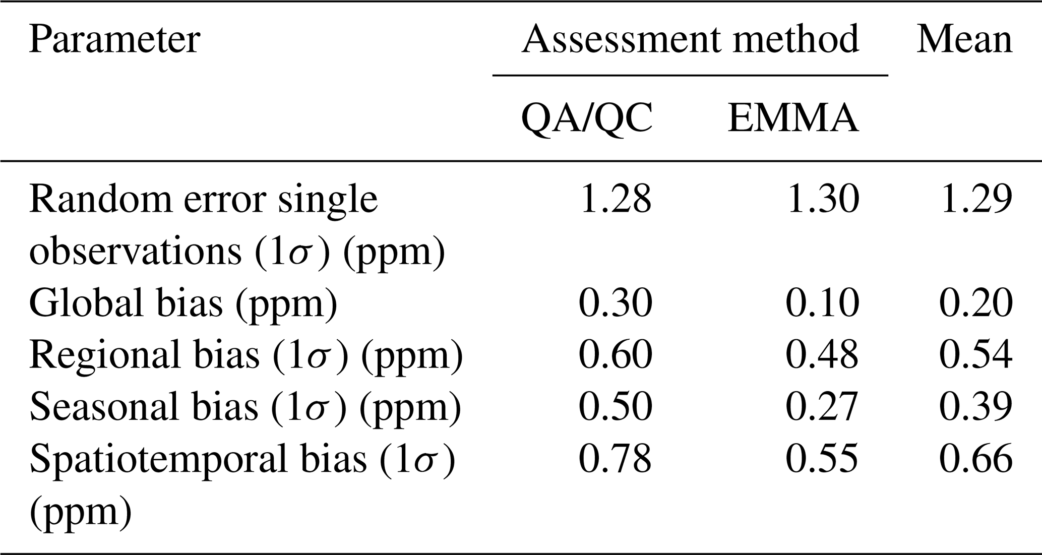
Table 5 lists (i) the mean value of the single-observation random error, (ii) the global bias computed as the mean value of the biases at the various TCCON sites, (iii) the regional bias computed as the standard deviation of the biases at the various TCCON sites, (iv) the mean seasonal bias, and (v) the spatiotemporal bias computed as the root sum square of the regional and of the seasonal bias. The spatiotemporal bias is used to quantify the achieved performance for relative accuracy, which characterizes the spatially and temporally varying component of the bias (i.e., neglects a possible global bias (global offset), which is reported separately).

The linear bias trend has also been computed by fitting a line to the satellite–TCCON differences (not shown here). The mean value of the linear trend (slope) and its uncertainty (1σ, obtained from the standard deviation of the slope at the various TCCON sites) are $-\mathrm{0.05}\pm \mathrm{0.06}$ ppm yr⁻¹ for the EMMA method and $-\mathrm{0.06}\pm \mathrm{0.09}$ ppm yr⁻¹ for the QA/QC method. This means that no significant long-term bias trend has been detected; i.e., the satellite product is stable.

As can be seen from Table 5, the values computed independently using the EMMA and the QA/QC assessment methods are quite similar, which gives not only confidence in the overall quality assessment summary documented in Table 5 but also in the products and the used validation methods.

Table 6 TCCON XCO₂ bias in parts per million (ppm; satellite – TCCON). “–” means that the number of available colocations is less than the threshold required by the corresponding assessment method. Note that this table includes only a subset of the 10 sites shown in Fig. 12, namely only those sites with a mean bias being considerably (more than 1.5 times) larger than the standard deviation of the biases.

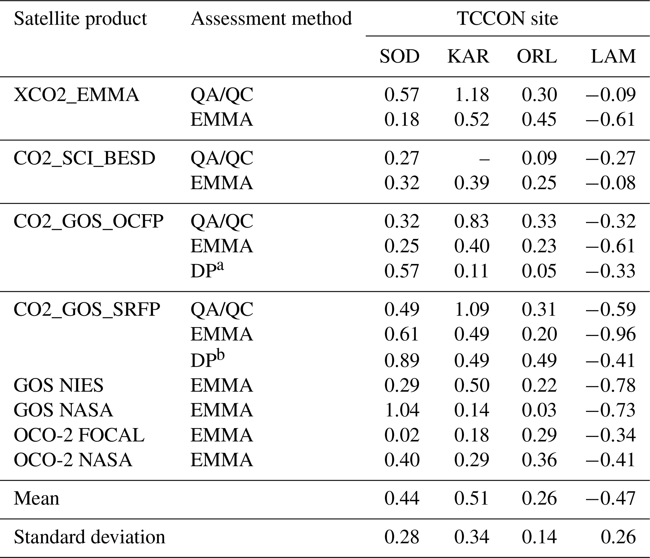
Assessment method DP is the method used by the data provider. For ^a see Boesch et al. (2019). For ^b see Wu et al. (2019).

Note however that the quality of the satellite data (at least at TCCON sites) is very likely better than Table 5 suggests (i) because the TCCON retrievals are not free of errors (the 1σ XCO₂ uncertainty is about 0.4 ppm; Wunch et al., 2010) and (ii) because of the representation error originating from the (real) spatiotemporal variability of XCO₂ around the TCCON sites. The overall error related to this is difficult to quantify, but some indication can potentially be obtained by additional assessment results such as the one shown in Fig. 12. Figure 12 shows the biases as obtained with the EMMA method at the various TCCON sites used for the EMMA method comparisons. Shown are not only the mean satellite–TCCON differences as obtained for the EMMA product but also for all the individual sensor/algorithm input products. The differences are shown as anomalies with respect to the mean; i.e., the sum of the differences in each row is zero. This is equivalent to assuming that for a given satellite product the mean value over all TCCON sites is zero. As can be seen from Fig. 12, the satellite–TCCON differences are dominantly positive (orange and red colors) for higher-latitude TCCON sites and mostly negative (blue colors) for lower-latitude TCCON sites. In order to rule out that this is an artifact of the EMMA assessment method, the overall biases computed with the QA/QC method and biases computed by the individual product data providers (DPs) have also been derived. These biases have been used to compute – for each of the 10 TCCON sites shown in Fig. 12 – the mean bias and the standard deviation of these biases. For 4 of these 10 sites the mean bias is considerably (more than 1.5 times) larger than the standard deviation of the biases, and the corresponding results for these four sites are shown in Table 6. This does not necessarily mean that these sites have the largest biases. This only means that the derived biases at these sites are (independent of their magnitude) the most consistent across all satellite products used for comparison. As can be seen from Table 6, the biases are always positive at Sodankylä, Karlsruhe, and Orléans and always negative at Lamont. Note that this does not imply that all derived biases are significant as some biases are very small, e.g., the FOCAL bias at Sodankylä, which is only 0.02 ppm. Because it is unlikely that all three satellites and several retrieval algorithms produce XCO₂ products with similar biases at a given TCCON site, this provides an indication of biases either due to representation errors or due to biases within the TCCON data (Table 6). Note that these biases are within the accuracy stated by TCCON, which is 0.8 ppm (2σ) (Wunch et al., 2010, Hedelius et al., 2017). The accuracy of the TCCON data will be improved for the next data release (planned for 2020). This new TCCON data set will allow for better identification of the causes for the observed biases.

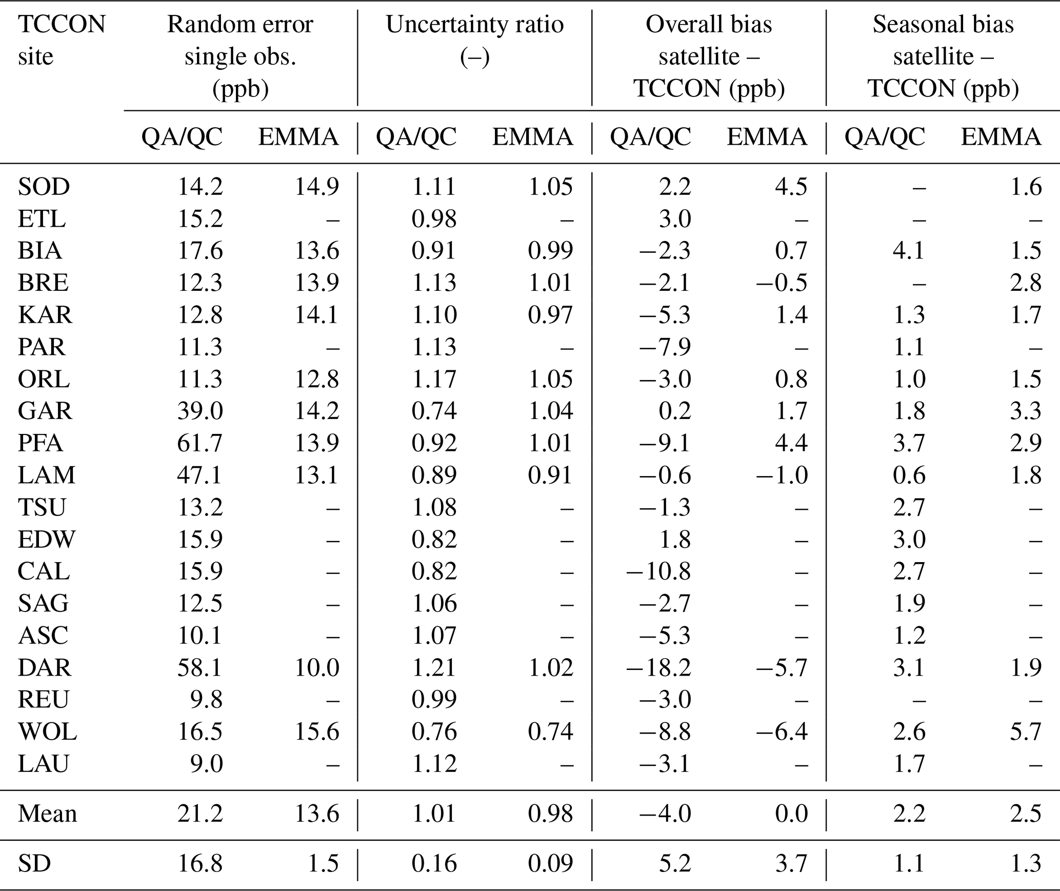
Table 7 Overview validation results at TCCON sites for data product XCH4_EMMA (version 4.1).

The XCO2_OBS4MIPS product has also been directly compared with TCCON using a comparison method based on the comparison of the monthly satellite product with TCCON monthly mean values. The results are shown in Fig. 13. As can be seen, the mean difference (satellite – TCCON) is 0.18 ppm (which is close to the mean value of the global bias of 0.20 ppm listed in Table 5), the standard deviation is 1.18 ppm (as expected, because of the spatiotemporal averaging, which is somewhat smaller than the value of 1.29 ppm obtained for the XCO2_EMMA product listed in Table 5), and the linear correlation coefficient is 0.99. The spatiotemporal bias, computed as the standard deviation of 3-monthly averages at the TCCON sites listed in Fig. 13, is 0.7 ppm.

Figure 1 presents an overview of the XCO₂ data product in terms of time series for three latitude bands and global maps. XCO₂ is increasing almost linearly during the 16-year time period (for a discussion of the derived annual growth rates see Sect. 4.3). The main reason for this increase is CO₂ emission due to burning of fossil fuels (Le Quéré et al., 2018). The seasonal cycle, which is caused primarily by quasi-regular uptake and release of atmospheric CO₂ by the terrestrial vegetation due to photosynthesis and respiration (e.g., Kaminski et al., 2017, Yin et al., 2018), is most pronounced over the Northern Hemisphere. The half-yearly maps for 2003 are based on SCIAMACHY on board ENVISAT (Burrows et al., 1995; Bovensmann et al., 1999) satellite data, and the maps for 2018 contain data from the GOSAT (since 2009) (Kuze et al., 2016) and OCO-2 (since 2014) (Crisp et al., 2004) satellites. GOSAT and OCO-2 also provide good-quality XCO₂ retrievals over the oceans due to their sunglint observation mode.

4.2 Products XCH4_EMMA and XCH4_OBS4MIPS (v4.1)

As for XCO₂, monthly maps have also been generated for the EMMA XCH₄ data product. Two examples are shown in Fig. 14 for September 2010 and in Fig. 15 for September 2018. The individual sensor XCH₄ input data are shown in the first four rows, and the EMMA XCH₄ product is shown in the bottom-left panel. The bottom-right panel shows the IAS. As can be seen, the spatial patterns of the XCH₄ maps are similar but not identical. The IAS shows a quite large variability. The scatter is larger compared to the corresponding XCO₂ IAS (Figs. 9 and 10, bottom-right panels), and spatially the grid cells with larger spread are more equally distributed over the globe but with largest differences over the southern part of Asia.

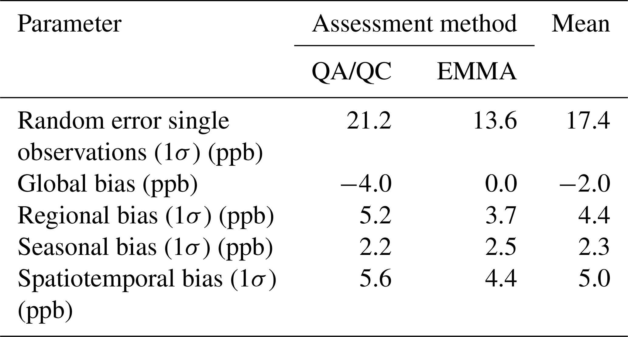
Detailed validation results are shown in Appendix A (Fig. A2), and the validation results are summarized in Tables 7 and 8, which have the same structure as the corresponding XCO₂ tables (Tables 4 and 5). These tables also list the results of the QA/QC assessment method, which results in quite similar (within a few ppb) overall quality assessment results (Table 8) as obtained with the EMMA method. The linear bias trend has also been computed by fitting a line to the satellite–TCCON differences (not shown here). The mean value of the linear trend (slope) and its uncertainty (1σ, obtained from the standard deviation of the slope at the various TCCON sites) are $-\mathrm{0.1}\pm \mathrm{0.4}$ ppb yr⁻¹ for the EMMA method and 0.5±0.8 ppb yr⁻¹ for the QA/QC method. As for XCO₂, this means that no significant long-term bias trend has been detected; i.e., the satellite product is stable.

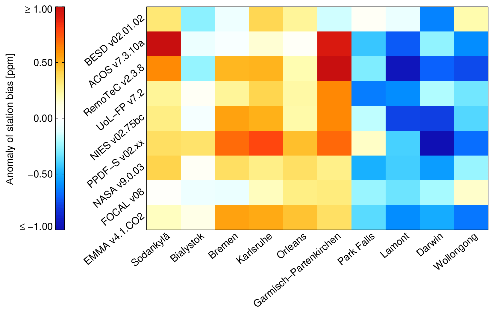
Figure 12 Average XCO₂ differences (satellite – TCCON) for the different satellite XCO₂ products at 10 TCCON sites as used by the EMMA assessment method. The differences are shown as anomalies; i.e., the sum of the values corresponding to a given row is zero. Note that here “ACOS” refers to NASA's ACOS algorithm as applied to GOSAT and that “NASA” refers to NASA's ACOS algorithm as applied to OCO-2.

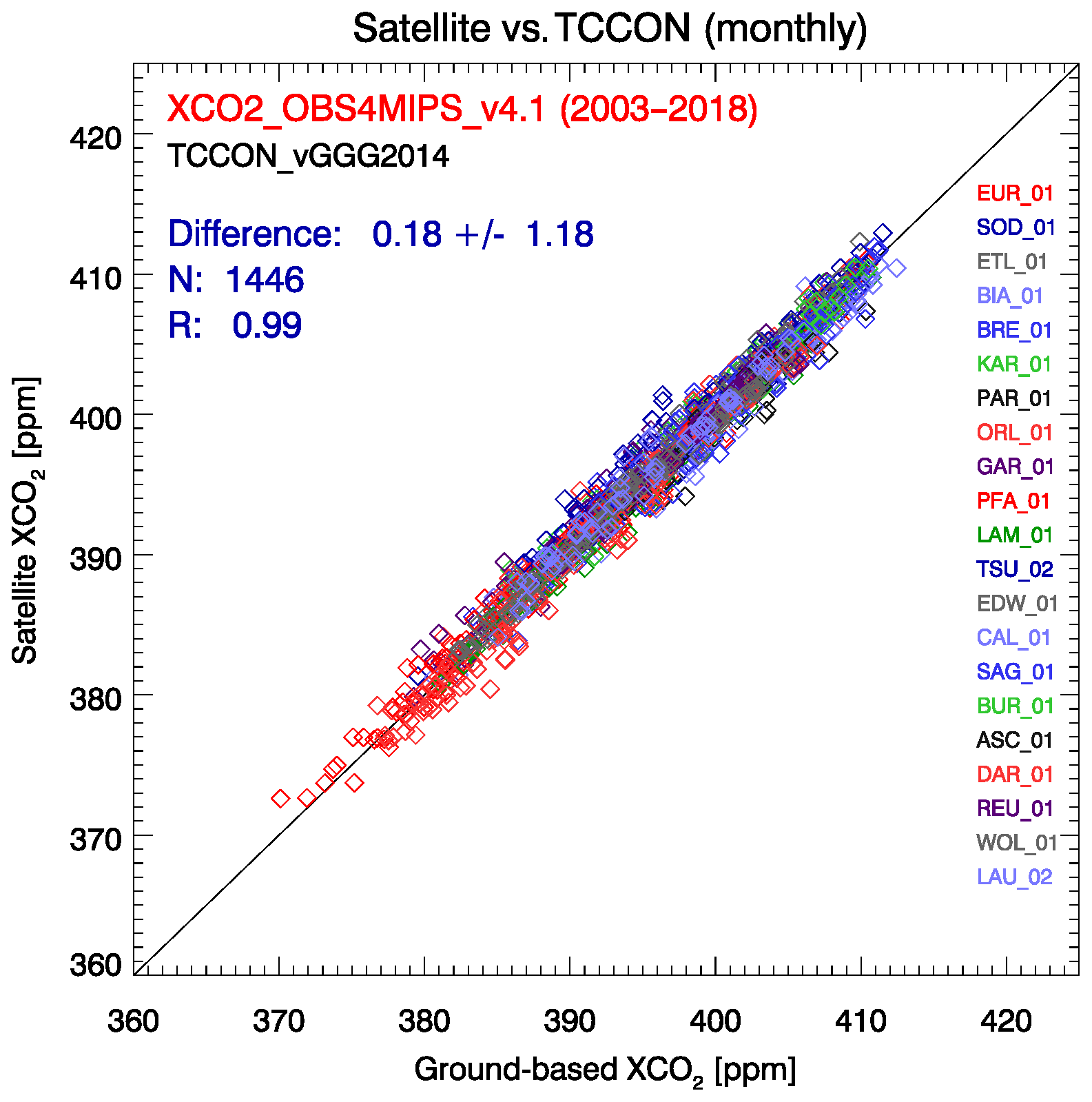
Figure 13 Summary of the comparison of product XCO2_OBS4MIPS with TCCON monthly mean XCO₂ (each symbol corresponds to one month and to one TCCON site; each color corresponds to a different TCCON site; TCCON site colors and site IDs (see Table 3) are shown on the right). The comparison is based on 1446 monthly values. The mean difference (satellite – TCCON) is 0.18 ppm and the standard deviation of the difference is 1.18 ppm. The linear correlation coefficient R is 0.99.

Figure 14 September 2010 XCH₄ at $\mathrm{10}{}^{\circ }\times \mathrm{10}{}^{\circ }$ spatial resolution showing (i) the individual sensor/algorithm input data sets (panels in rows 1–4; see Table 2 for details), (ii) EMMA XCH₄ (bottom left), and (iii) the inter-algorithm spread (IAS, 1σ) as computed by EMMA (bottom right; see main text for details). Also shown in the bottom-right panel are the locations of the TCCON sites (pink triangles) and the range of IAS values covered by them (see color bar).

Figure 16 shows the TCCON station XCH₄ bias anomaly as also shown for XCO₂ in Fig. 12; i.e., Fig. 16 shows the biases as obtained with the EMMA method at the various TCCON sites used for the EMMA method comparisons. As for XCO₂ not only the mean satellite–TCCON differences as obtained for the EMMA product are shown but also the differences for all the individual sensor/algorithm input products. The differences are shown as anomalies with respect to the mean; i.e., the sum of the differences in each row is zero. As can be seen from Fig. 16, the pattern of satellite–TCCON XCH₄ differences has some similarity with the XCO₂ difference pattern shown in Fig. 12. For example, the differences are mostly positive at Sodankylä and Garmisch-Partenkirchen and mostly negative at Darwin and Wollongong. But there are also significant differences, for example, with respect to the sign of the bias (e.g., Park Falls, Bremen, Karlsruhe).

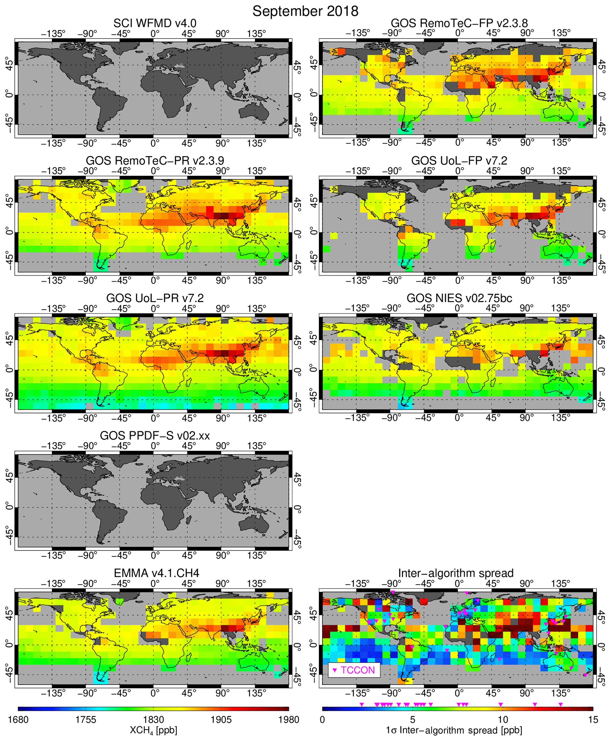
Figure 15 As Fig. 14 but for September 2018. Note that the SCIAMACHY/WFMD map (top left) is empty because this product ended in April 2012 (see Fig. 14 for SCIAMACHY/WFMD XCH₄). For product GOSAT/PPDF (row 4) no data were available for this month (see Fig. 14 for GOSAT/PPDF XCH₄).

Table 8 Validation summary for data product XCH4_EMMA (version 4.1).

The XCH4_OBS4MIPS product has also been directly compared with TCCON (Fig. 17) using the same method as also used for product XCO2_OBS4MIPS (Fig. 13). As can be seen from Fig. 17, the mean difference (satellite – TCCON) is −2.88 ppb (which is close to the mean value of the global bias of −2.0 ppb of product XCH4_EMMA listed in Table 8), the standard deviation is 8.65 ppb (as expected, because of the averaging, which is somewhat smaller than the value of 17.4 ppb obtained for the XCH4_EMMA product listed in Table 8), and the linear correlation coefficient is 0.97.

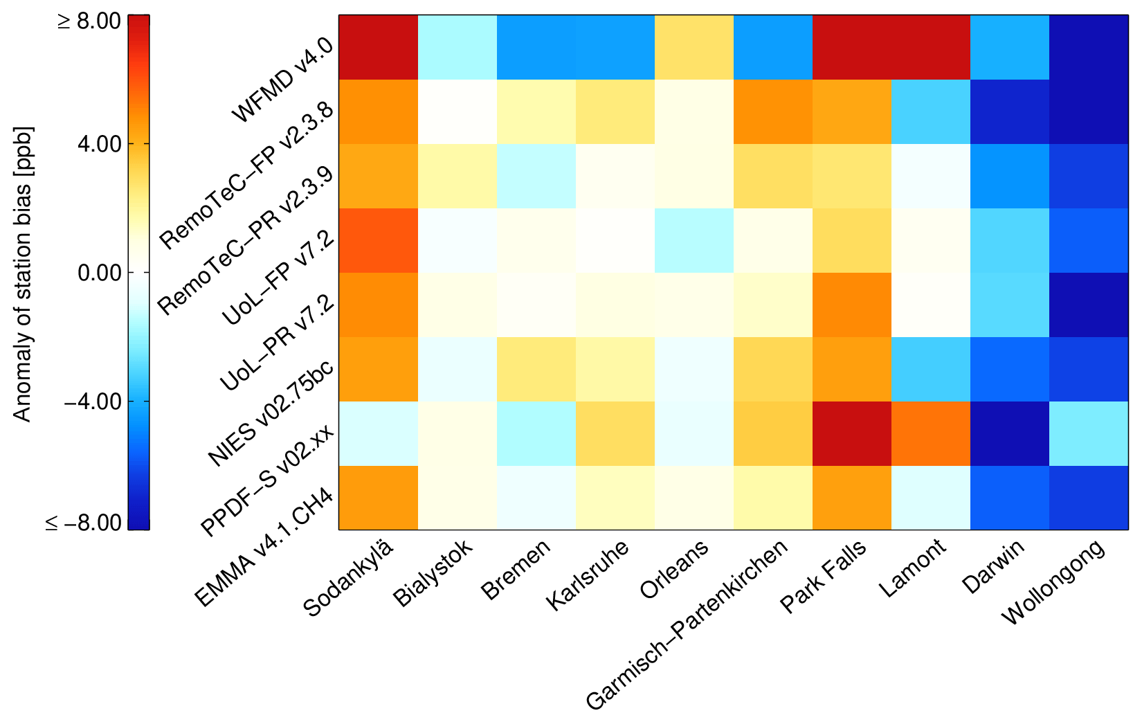
Figure 16 As Fig. 12 but for XCH₄, i.e., average XCH₄ differences (satellite – TCCON) for the different satellite XCH₄ products at 10 TCCON sites as used by the EMMA assessment method. The differences are shown as anomalies; i.e., the sum of the values corresponding to a given row is zero.

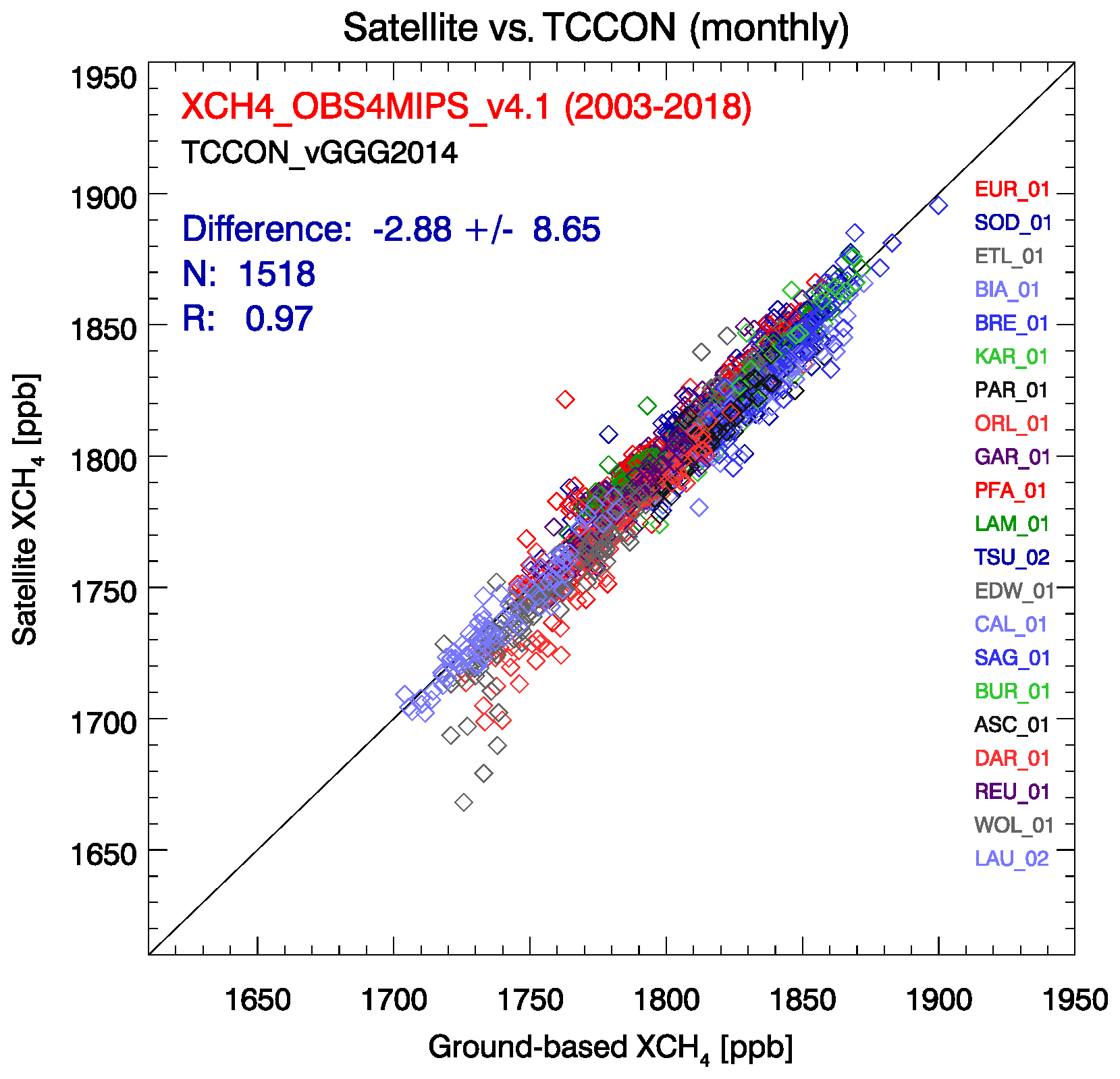
Figure 17 Summary of the comparison of product XCH4_OBS4MIPS with TCCON monthly mean XCH₄. The comparison is based on 1518 monthly values. The mean difference (satellite – TCCON) is −2.88 ppb and the standard deviation of the difference is 8.65 ppb. The linear correlation coefficient R is 0.97.

Figure 2 presents an overview of the XCH₄ data product in terms of time series for three latitude bands and global maps. As can be seen, XCH₄ was nearly constant during 2003–2006 (apart from seasonal fluctuations) but has been increasing since 2007 (for a discussion of the trend and annual growth rates see Sect. 4.3). The reason for this is likely a combination of increasing natural (e.g., wetlands) and anthropogenic (e.g., fossil fuel related) emissions and possibly decreasing sinks (hydroxyl, OH, radical), but it does not seem currently possible to be more definitive (e.g., Worden et al., 2017; Nisbet et al., 2019; Turner et al., 2019; Howarth, 2019; Schaefer, 2019).

4.3 Annual growth rates

Finally, we present an update and extension of the year 2003–2016 annual XCO₂ growth rates shown in Buchwitz et al. (2018), using the new OBS4MIPS v4.1 XCO₂ data set covering the time period 2003–2018 (Fig. 18). Figure 18a shows the time series of the globally averaged OBS4MIPS version 4.1 XCO₂ data product over land. In contrast to Buchwitz et al. (2018), the analysis presented here is based on data over land only as this permits the generation of a time series with better internal consistency (note that the XCO₂ OBS4MIPS product is land only for 2003–2008). The average growth rate during 2010–2018, i.e., for the time period where an ensemble of GOSAT and OCO-2 data has been used, is 2.28±0.04 ppm yr⁻¹. As can be seen from Fig. 18b, the year 2017 and 2018 growth rates are less than the growth rates of the years 2015 and 2016, which were years with a strong El Niño. The XCO₂ growth rates are in reasonable agreement with the global CO₂ growth rates published by National Oceanic and Atmospheric Administration (NOAA) (shown in blue color in Fig. 18b), which are based on marine surface CO₂ observations (ftp://aftp.cmdl.noaa.gov/products/trends/co2/co2_gr_gl.txt; last access: 30 July 2019). As can be seen from Fig. 18b, the agreement of the satellite-derived XCO₂ growth rates with the NOAA surface-CO₂-based growth rates is better from year 2010 onwards compared to the time period before when the EMMA data set consists only of one SCIAMACHY data set instead of the full ensemble. For 2018, the XCO₂ growth rate is 2.1±0.5 ppm yr⁻¹, which is lower than the NOAA surface CO₂ growth rate of 2.43±0.08 ppm yr⁻¹. Note that the 1σ uncertainty ranges of the two growth rate estimates overlap, which indicates that the two growth rate estimates are consistent.

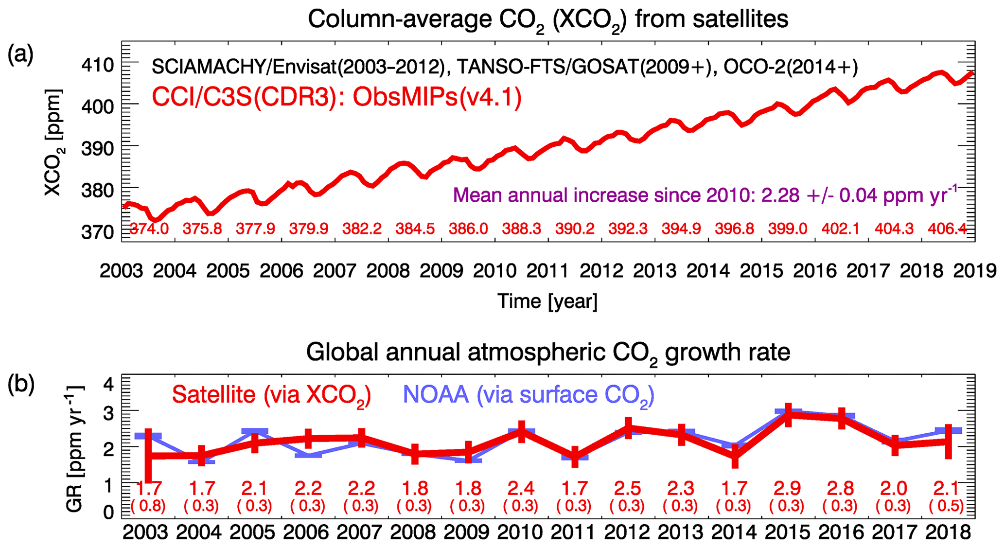
Figure 18 (a) Monthly values of the globally averaged XCO₂ (over land) as computed from the OBS4MIPS version 4.1 XCO₂ data product. The corresponding annual mean XCO₂ values are also listed. The increase during 2010–2018 is 2.28±0.04 ppm yr⁻¹ as obtained via a linear fit. (b) Annual XCO₂ growth rates (red, with 1σ uncertainties; the corresponding numerical values are also listed with 1σ uncertainty in brackets) and CO₂ growth rates from NOAA (shown in blue) obtained from marine surface CO₂ observations.

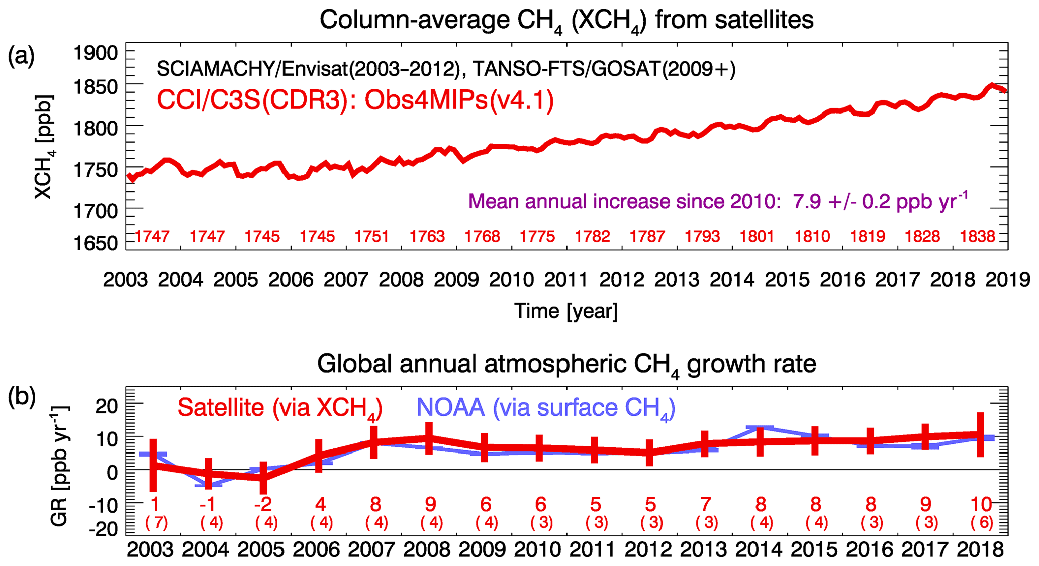
Figure 19 (a) Monthly values of the globally averaged XCH₄ (over land) as computed from the OBS4MIPS version 4.1 XCH₄ data product. The corresponding annual mean XCH₄ values are also listed. The increase during 2010–2018 is 7.9±0.2 ppb yr⁻¹ as obtained via a linear fit. (b) Annual XCH₄ growth rates (red, with 1σ uncertainties; the corresponding numerical values are also listed with 1σ uncertainty in brackets) and CH₄ growth rates from NOAA (shown in blue) obtained from marine surface CH₄ observations.

The growth rate of atmospheric methane is also an important quantity (e.g., Nisbet et al., 2019). The method of Buchwitz et al. (2018) has now also been used to compute annual XCH₄ growth rates from satellite XCH₄ retrievals. Figure 19a shows the time series of the globally averaged OBS4MIPS version 4.1 XCH₄ data product over land. As shown by the linear fit, the average growth rate is 7.9±0.2 ppb yr⁻¹ during 2010–2018, i.e., for the time period where an ensemble of GOSAT data has been used. The annual growth rates are shown in Fig. 19b for the satellite-derived XCH₄ (red) and for the NOAA growth rates (ftp://aftp.cmdl.noaa.gov/products/trends/ch4/ch4_gr_gl.txt; last access: 30 July 2019) derived from marine surface CH₄ observations. For 2018, the XCH₄ growth rate is 10±6 ppb yr⁻¹, which is close to the NOAA surface CH₄ growth rate of 9.46±0.56 ppb yr⁻¹.

5 Summary and conclusions

Satellite-derived ensemble XCO₂ and XCH₄ data products have been generated and validated. These data products are the version 4.1 Level 2 (L2) products XCO2_EMMA and XCH4_EMMA and the Level 3 (L3) products XCO2_OBS4MIPS and XCH4_OBS4MIPS and cover the time period 2003–2018. The data products are freely available for interested users via the Copernicus Climate Data Store (CDS, https://cds.climate.copernicus.eu/, last access: 10 January 2020), where also earlier versions of these data products are accessible. The L2 products have been generated with an adapted version of the EMMA algorithm (Reuter et al., 2013), and the L3 products have been generated by gridding (averaging) the EMMA L2 product to obtain products at monthly time and $\mathrm{5}{}^{\circ }\times \mathrm{5}{}^{\circ }$ spatial resolution in Obs4MIPS format. The products have been validated by comparisons with TCCON ground-based XCO₂ and XCH₄ retrievals using TCCON version GGG2014.

From January 2003 to March 2009 the products are based on SCIAMACHY/ENVISAT, and from April 2009 onwards the products use an ensemble of one SCIAMACHY (until early 2012) and several GOSAT products. The XCO₂ products contain in addition L2 products from NASA's OCO-2 mission from September 2014 onwards.

The EMMA algorithm selects for each month and each $\mathrm{10}{}^{\circ }\times \mathrm{10}{}^{\circ }$ grid cell one of the available products, i.e., one from the existing ensemble of L2 input products, and transfers all relevant information (including averaging kernel etc.) from the selected L2 input product into the merged EMMA L2 product. The selected product is the median product. The main purpose of EMMA is to generate a Level 2 product, which covers an as-long-as-possible time series (longer than any of the individual sensor input data sets) with as-high-as-possible accuracy including all information needed, e.g., for surface flux inverse modeling. The median approach helps to reduce the occurrence of potential outliers and thus reduces spatial and temporal biases in the generated data products.

Detailed quality assessment results based on comparisons with TCCON ground-based retrievals have been presented. We found that the XCO₂ Level 2 data set at the TCCON validation sites can be characterized by the following figures of merit (the corresponding values for the Level 3 product are listed in brackets) – single-observation random error (1σ): 1.29 ppm (monthly: 1.18 ppm); global bias: 0.20 ppm (0.18 ppm); and spatiotemporal bias or relative accuracy (1σ): 0.66 ppm (0.70 ppm). The corresponding values for the XCH₄ products are single-observation random error (1σ): 17.4 ppb (monthly: 8.7 ppb); global bias: −2.0 ppb (−2.9 ppb), spatiotemporal bias (1σ): 5.0 ppb (4.9 ppb). It has also been found that the data products exhibit very good long-term stability as no significant linear bias trends have been identified.

The new data sets have also been used to derive annual XCO₂ and XCH₄ growth rates, which are in reasonable to good agreement with growth rates from the National Oceanic and Atmospheric Administration (NOAA) based on marine surface observations.

An important application for the EMMA products is to use them together with inverse modeling to obtain improved information on regional-scale CO₂ (e.g., Houweling et al., 2015) and CH₄ (e.g., Alexe et al., 2015) surface fluxes. Applications for the corresponding OBS4MIPS products are, for example, climate model comparisons (e.g., Lauer et al., 2017) and studies related to annual growth rates (e.g., Buchwitz et al., 2018). It is however important to note that these merged products are not necessarily the most optimal products for all applications as they do not contain all data from a given satellite sensor. For example, users interested primarily in emissions from power plants or other localized CO₂ sources will prefer the original OCO-2 Level 2 data product (e.g., Nassar et al., 2017; Reuter et al., 2019a). Especially for users interested in only parts of the time series it is recommended to use the individual sensor products in addition to the merged product as this may significantly increase the robustness, reliability, and uncertainty characterization of key findings.

Appendix A

In this appendix, detailed validation results are shown for the individual sensor and EMMA XCO₂ and XCH₄ Level 2 data products.

The comparison of the various XCO₂ data products with TCCON XCO₂ at 10 TCCON sites is shown in Fig. A1. These 10 TCCON sites fulfill the EMMA criteria in terms of a sufficiently large number of colocations as defined to obtain robust conclusions per site. The individual soundings of the EMMA XCO₂ product are shown as white circles with a black border. As can be seen, they are located within (mostly close to the center of) the range of values of the individual sensor/algorithm XCO₂ values, which is expected.

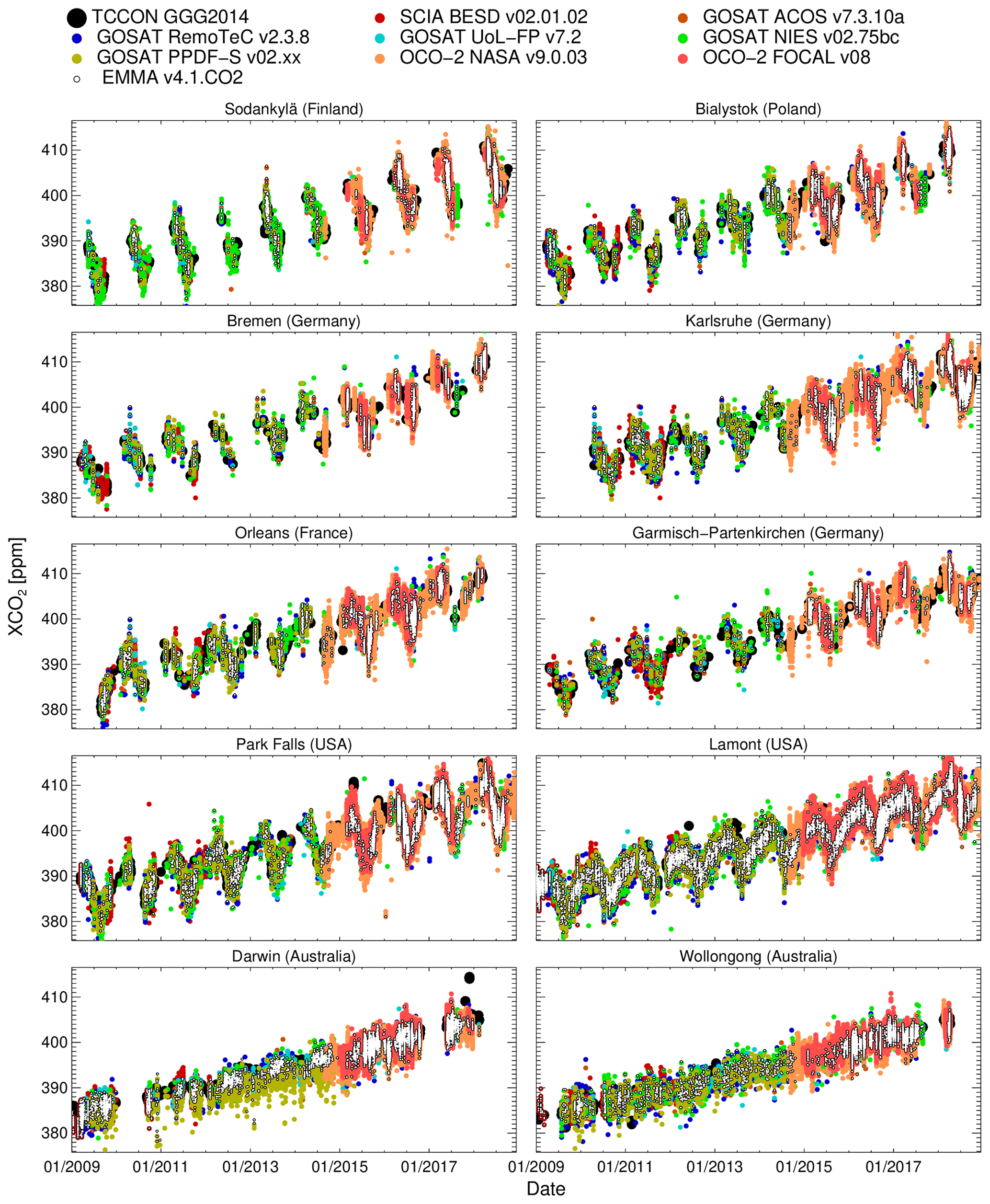
Figure A1 XCO₂ time series at 10 TCCON sites during January 2009–December 2018 as obtained using the EMMA quality assessment method. TCCON GGG2014 XCO₂ is shown as thick black dots, the individual satellite L2 input products are shown as colored dots, and the EMMA product is shown as white circles with black borders. The derived numerical values are listed in Table 4.

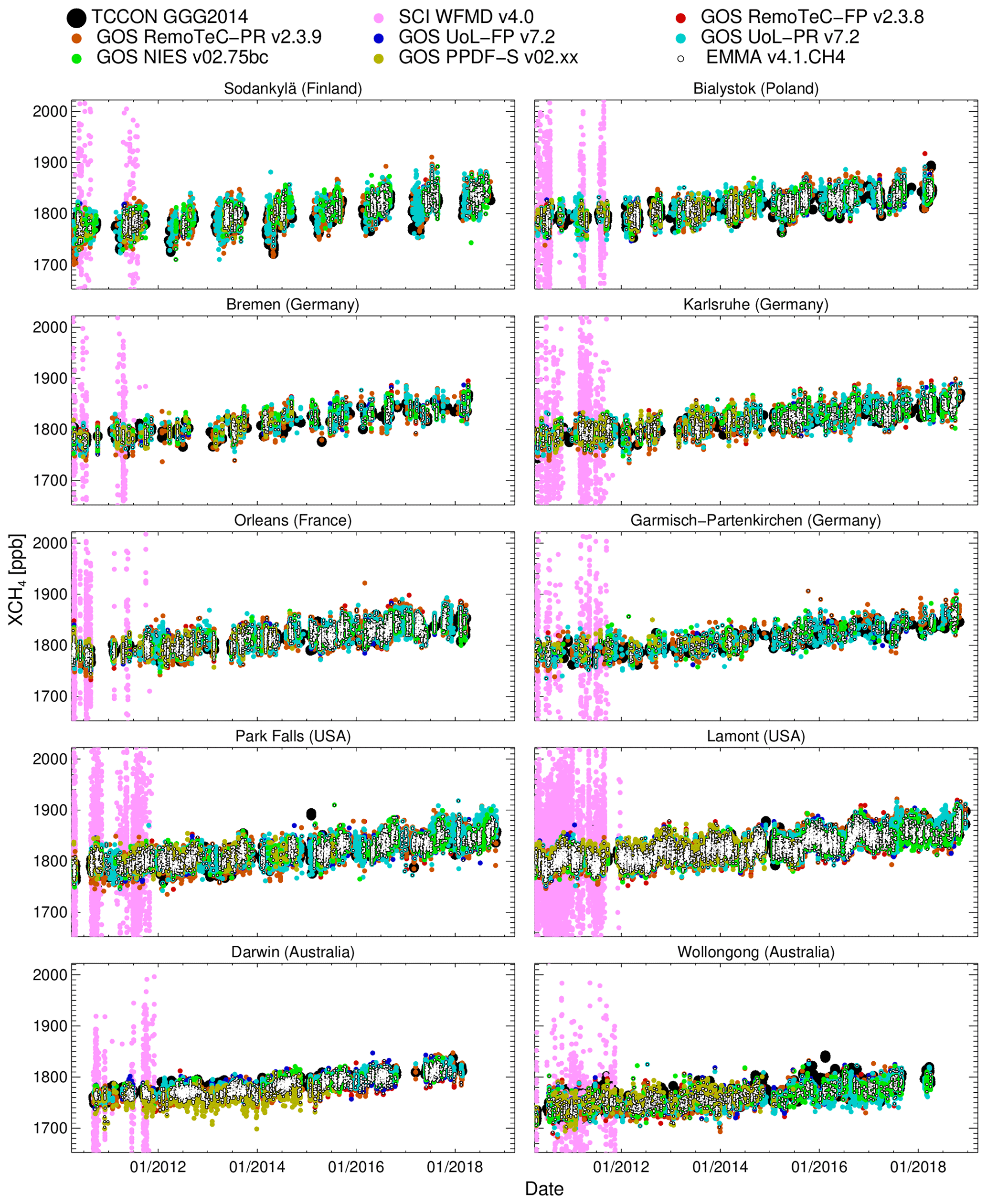
Figure A2 XCH₄ time series at 10 TCCON sites during April 2010–December 2018 as obtained using the EMMA quality assessment method. TCCON GGG2014 XCH₄ is shown as thick black dots, the individual satellite L2 input products are shown as colored dots, and the EMMA product is shown as a white circles with black borders. The derived numerical values are listed in Table 7.

Figure A2 shows the comparison of the EMMA XCH₄ product (white circles with a black border) and of the individual sensor XCH₄ input products with TCCON XCH₄ originating from the EMMA assessment method. As for the EMMA XCO₂ product (Fig. A1), the EMMA XCH₄ is located near the center of the clouds of XCH₄ values, as expected.