the Creative Commons Attribution 4.0 License.
the Creative Commons Attribution 4.0 License.
 | 24 Feb 2021
Characterizing water vapour concentration dependence of commercial cavity ring-down spectrometers for continuous on-site atmospheric water vapour isotope measurements in the tropics
Fumiyoshi Kondo
Heiko Moossen
Thomas Seifert
Uwe Schultz
Heike Geilmann
David Walter
Jost V. Lavric
The recent development and improvement of commercial laser-based spectrometers have expanded in situ continuous observations of water vapour (H2O) stable isotope compositions (e.g. δ18O and δ2H) in a variety of sites worldwide. However, we still lack continuous observations in the Amazon, a region that significantly influences atmospheric and hydrological cycles on local to global scales. In order to achieve accurate on-site observations, commercial water isotope analysers require regular in situ calibration, which includes the correction of H2O concentration dependence ([H2O] dependence) of isotopic measurements. Past studies have assessed the [H2O] dependence for air with H2O concentrations of up to 35 000 ppm, a value that is frequently surpassed in tropical rainforest settings like the central Amazon where we plan continuous observations. Here we investigated the performance of two commercial analysers (L1102i and L2130i models, Picarro, Inc., USA) for measuring δ18O and δ2H in atmospheric moisture at four different H2O levels from 21 500 to 41 000 ppm. These H2O levels were created by a custom-built calibration unit designed for regular in situ calibration. Measurements on the newer analyser model (L2130i) had better precision for δ18O and δ2H and demonstrated less influence of H2O concentration on the measurement accuracy at each concentration level compared to the older L1102i. Based on our findings, we identified the most appropriate calibration strategy for [H2O] dependence, adapted to our calibration system. The best strategy required conducting a two-point calibration with four different H2O concentration levels, carried out at the beginning and end of the calibration interval. The smallest uncertainties in calibrating [H2O] dependence of isotopic accuracy of the two analysers were achieved using a linear surface fitting method and a 28 h calibration interval, except for the δ18O accuracy of the L1102i analyser for which the cubic fitting method gave the best results. The uncertainties in [H2O] dependence calibration did not show any significant difference using calibration intervals from 28 up to 196 h; this suggested that one [H2O] dependence calibration per week for the L2130i and L1102i analysers is sufficient. This study shows that the cavity ring-down spectroscopy (CRDS) analysers, appropriately calibrated for [H2O] dependence, allow the detection of natural signals of stable water vapour isotopes at very high humidity levels, which has promising implications for water cycle studies in areas like the central Amazon rainforest and other tropical regions.
- Article
(5767 KB) - Full-text XML
-
Supplement
(503 KB) - BibTeX
- EndNote


Ongoing climate change has affected various aspects of global and local climate, including the hydrological cycle (Bindoff et al., 2013). Further and more detailed understanding on how climate change affects the atmospheric hydrological system is required. Water vapour isotope compositions (e.g. δ18O, δ2H, δ17O) have been used in meteorology and hydrology to disentangle the water vapour transport, mixing, and phase changes such as evaporation and condensation that govern processes of the atmospheric hydrological cycle (Dansgaard, 1964; Craig and Gordon, 1965; Galewsky et al., 2016). Incorporating water vapour isotopic information into global and regional circulation models has also improved our understanding of how stable water isotopes are transported in the atmosphere and affected by phase changes in and below clouds and how they behave in different situations of surface–atmosphere interactions (Risi et al., 2010; Werner et al., 2011; Pfahl et al., 2012). The increase in field observations of water vapour isotope compositions therefore is expected to improve our process understanding and thereby models simulating the interactions between the atmospheric hydrological system and global climate change.
Until around 10–15 years ago, in situ water vapour isotope measurements were limited due to the laborious and error-prone sampling techniques using cryogenic traps, molecular sieves, and vacuum flasks, etc. (Helliker and Noone, 2010). Recent development and improvement of laser-based spectrometers have made continuous water vapour isotope composition measurements at a high temporal resolution possible. The number of on-site measurements of stable water vapour isotope compositions across the world has increased in the last decade (Wei et al., 2019). So far, there are many studies based on field water isotopic measurements available in polar and mid-latitude regions, some in the subtropics (e.g. Bailey et al., 2013; Gonzalez et al., 2016) but only very few in the tropics (e.g. Tremoy et al., 2012; Aemisegger et al., 2020). Particularly studies in tropical continental regions, such as the Amazon basin region, are rare. Yet, understanding the hydrological processes in the Amazon basin is crucial as it significantly influences the atmospheric convective circulation in the tropics and beyond (Coe et al., 2016; Galewsky et al., 2016). Thus, in situ continuous measurements of water vapour isotope compositions in the Amazon region will improve our comprehension of the Amazonian hydro-climatological system and its interaction with global climate (Coe et al., 2016; Galewsky et al., 2016).
Recent field observations for water vapour isotopes have mainly utilized two commercial laser-based instruments: Picarro cavity ring-down spectroscopy (CRDS) and Los Gatos Research off-axis integrated cavity output spectroscopy (OA-ICOS) analysers (Galewsky et al., 2016; Wei et al., 2019). The CRDS analysers have been used in most of the field sites that are registered on the Stable Water Vapor Isotopes Database (SWVID) website that archives on-site high-frequency water vapour isotope data (Wei et al., 2019). Globally, five Picarro CRDS models (i.e. L1102i, L1115i, L2120i, L2130i, and L2140i, sorted by oldest to newest) are in operation at various field sites. Aemisegger et al. (2012) demonstrated that a recent model (L2130i) has better precision and accuracy compared to an older model (L1115i) due to the improved spectroscopic fitting algorithms.
Even with improved analysers, CRDS instruments still require regular calibration (e.g. 3–24 h frequency) (Aemisegger et al., 2012; Delattre et al., 2015; Wei et al., 2019). The main calibration issue is that the measurement quality of water vapour isotopic compositions depends on water vapour (H2O) concentration (hereinafter called “[H2O] dependence”; Schmidt et al., 2010; Tremoy et al., 2011; Aemisegger et al., 2012; Bailey et al., 2015; Delattre et al., 2015). The [H2O] dependence of Picarro analysers has been assessed over a H2O concentration range spanning 200 to 35 000 ppm (Schmidt et al., 2010; Aemisegger et al., 2012; Steen-Larsen et al., 2014; Bailey et al., 2015; Delattre et al., 2015) and only rarely above 35 000 ppm (Tremoy et al., 2011).
However, H2O concentrations within the Amazon tropical rainforest canopy (e.g. the Amazon Tall Tower Observatory (ATTO) site; see Andreae et al., 2015) exceed 35 000 ppm on a daily basis and occasionally 40 000 ppm. In addition, Moreira et al. (1997) observed that the diel variation pattern in H2O concentration in the Amazon tropical rainforest was mostly similar to that in δ18O and δ2H of water vapour. The diel relationship between H2O concentration and isotopes may lead to over- or underestimation of isotopic values measured by CRDS analysers in the Amazon tropical rainforest. Thus, for in situ water vapour isotope measurements by CRDS analysers in the Amazon tropical rainforest, the [H2O] dependence of CRDS analysers under high moisture conditions (> 35 000 ppm H2O) needs to be assessed and corrected.
The primary aim of this study was to characterize two CRDS analysers (L1102i and L2130i) for measuring δ18O and δ2H of water vapour in high atmospheric moisture expected at the ATTO site (∼ 150 km NE of Manaus, Brazil), where we intend to conduct continuous in situ observations. Over a 2-week period, we examined the effects of H2O concentration on isotopic measurement precision and accuracy for both an old (L1102i) and a new CRDS model (L2130i). They were both connected to our custom-made calibration system that regularly supplied standard water vapour samples at four different H2O concentrations covering high moisture conditions (21 500 to 41 000 ppm). Standard water vapour samples were made from two standard waters, almost covering the previously reported isotopic ranges (δ18O = −19.4 ‰ to −6.7 ‰ and δ2H = −151 ‰ to −42 ‰) for water vapour samples from Manaus or from the Ducke Reserve near Manaus (Matsui et al., 1983; Moreira et al., 1997; IAEA/WMO, 2020). We also assessed which [H2O] dependence calibration strategy can best reduce measurement uncertainty of the two CRDS models. Based on the uncertainty quantification presented, we discussed whether the CRDS analysers with our calibration setup can sufficiently detect natural signals of stable water vapour isotopes expected at the ATTO site.
2.1 Calibration system
A setup with a commercial vaporizer coupled with a standard delivery module (A0211 and SDM, A0101, respectively; Picarro Inc., Santa Clara, CA, USA) guarantees the delivery of standard water vapour samples of up to 30 000 ppm of H2O, which does not cover the H2O concentration range we are expecting for the Amazon rainforest. In addition, according to discussion with Picarro's technicians, there is no easy way to run an A0101 with the L1102i model. Therefore, we built a calibration system to routinely and automatically conduct on-site calibration of CRDS analysers (Fig. 1). The main units of the calibration system are a syringe pump, a vaporizer and a dry-air supply unit (Fig. 1a). The syringe pump (Pump 11 Pico Plus Elite, Harvard Apparatus, Holliston, MA, USA) takes 3.3 mL standard water from a 2L reservoir bag (Cali-5-Bond™, Calibrated Instruments, Inc., Ardsley, New York, USA) and delivers the standard water into a vaporizer unit with a constant water flow of 1.9 µL min−1 (Fig. 1a and b). To maintain accuracy of the syringe pump's infusion over a long term, two guide rods and a lead screw of the syringe pump need to be properly lubricated every 100 h of operation (i.e. injecting and withdrawing). The vaporizer unit that was modified from an A0211 is comprised of a heater, vaporization chamber, and buffer reservoir, which is enclosed in a copper pipe and heated at 140 ∘C, covered by insulation material to reduce heat dissipation and help to reduce the memory effects between different water vapour isotopic measurements. Dried ambient air, recommended as a carrier gas for calibration by Aemisegger et al. (2012), was supplied into the heated vaporizer unit from a dry-air unit made up of a compressor, water separator, mist separators, membrane dryer (IDG60SAM4-F03C, SMC, Tokyo, Japan), precision regulator (IR1000, SMC, Tokyo, Japan) and flow regulator (Fig. 1a and c). We chose SMC's membrane dryer because SMC guarantees a long-term operation (e.g. 10 years or more by 10 h per day of operation) without replacing the membrane module. The dry-air unit and mass flow controller 1 (MFC1) (1179B, MKS GmbH, Munich, Germany) provide the vaporizer unit with a steady flow of dried ambient air with a dew point temperature of −32 ∘C or below (∼ 300 ppm of H2O or below), operated at 50 mL min−1 flow rate and 17.2–20.7 kPa flow pressure. The dry air entering the vaporizer is heated through the heater line, speeding up the evaporation of the infused standard water inside the vaporization chamber without fractionation. Furthermore, the heated carrier gas also helps to reduce the memory effect of the measurements. The subsequent standard water vapour was well mixed inside a bigger buffer reservoir compared to A0211. The customized heating system and buffer reservoir enabled us to produce a high moisture stream of standard water vapour samples, which were then delivered through the multiposition valve (Model EMTMA-CE, VICI Corp., Houston, TX, USA), switching flow paths between the calibration and routine analysis mode of the two CRDS analysers: L1102i and L2130i. To minimize tubing memory effects on water vapour isotopic measurements, we connected the vaporizer unit and CRDS analysers with stainless steel tubing constantly held at 45 ∘C with heating tape to avoid condensation inside the tubes (Schmidt et al., 2010; Tremoy et al., 2011). Before reaching the CRDS analysers, the transported standard water vapour was diluted with the dried ambient air via a dilution line and adjusted to an intended concentration level by regulating the dilution dry-air flow rate using MFC2. The total flow rate of both the calibration and dilution lines exceeded the suction flow rates of the two CRDS analysers (∼ 50 mL min−1 in total). The excess air was exhausted through an overflow port.
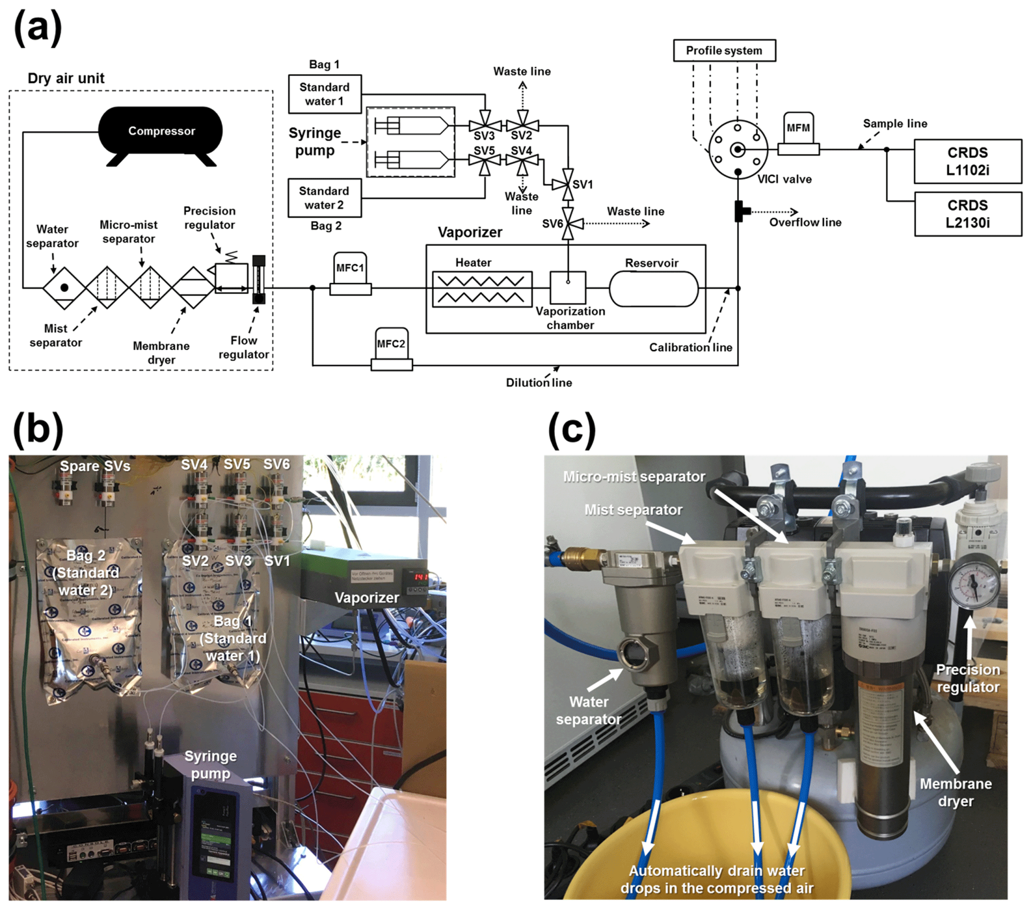
Figure 1(a) Schematic diagram of the calibration system, including the dry-air unit. MFC, MFM, and SV denote mass flow controller, mass flow meter, and three-way solenoid valve, respectively. The profile system, prepared for in situ observation at the Amazon Tall Tower Observatory site (see Andreae et al., 2015) in the Amazon tropical forest, is not described in this article. The diagram is not to scale. Panel (b) shows the photo of the main part of the calibration system: a vaporizer, syringe pump, 2 L reservoir bags, and solenoid valves. Panel (c) shows the photo of the main part of the dry-air unit: a water separator, mist separators, membrane dryer, precision regulator, and drain lines for water drops in the compressed air.
2.2 Water vapour concentration dependence experiment
We conducted a continuous operation of the L1102i and L2130i analysers over a 2-week period in June 2019 in an air-conditioned laboratory at the Max Planck Institute for Biogeochemistry (MPI-BGC, Jena, Germany). The two CRDS analysers measured water vapour (H2O) concentration, δ18O and δ2H of outside/room air samples from a profile gas-stream switching system (not shown here) or H2O concentration, δ18O and δ2H of water vapour samples supplied from the calibration system (Fig. 1a). Since H2O concentration values measured by old CRDS models (e.g. L1102i) are biased due to the self-broadening effect of water vapour (Winderlich et al., 2010; Rella et al., 2013), H2O concentration measurements by the L1102i were corrected by a non-linear calibration fitting, determined by Winderlich et al. (2010) and recommended for old CRDS models (e.g. G1301 CO2/CH4/H2O analyser) by Rella (2010).
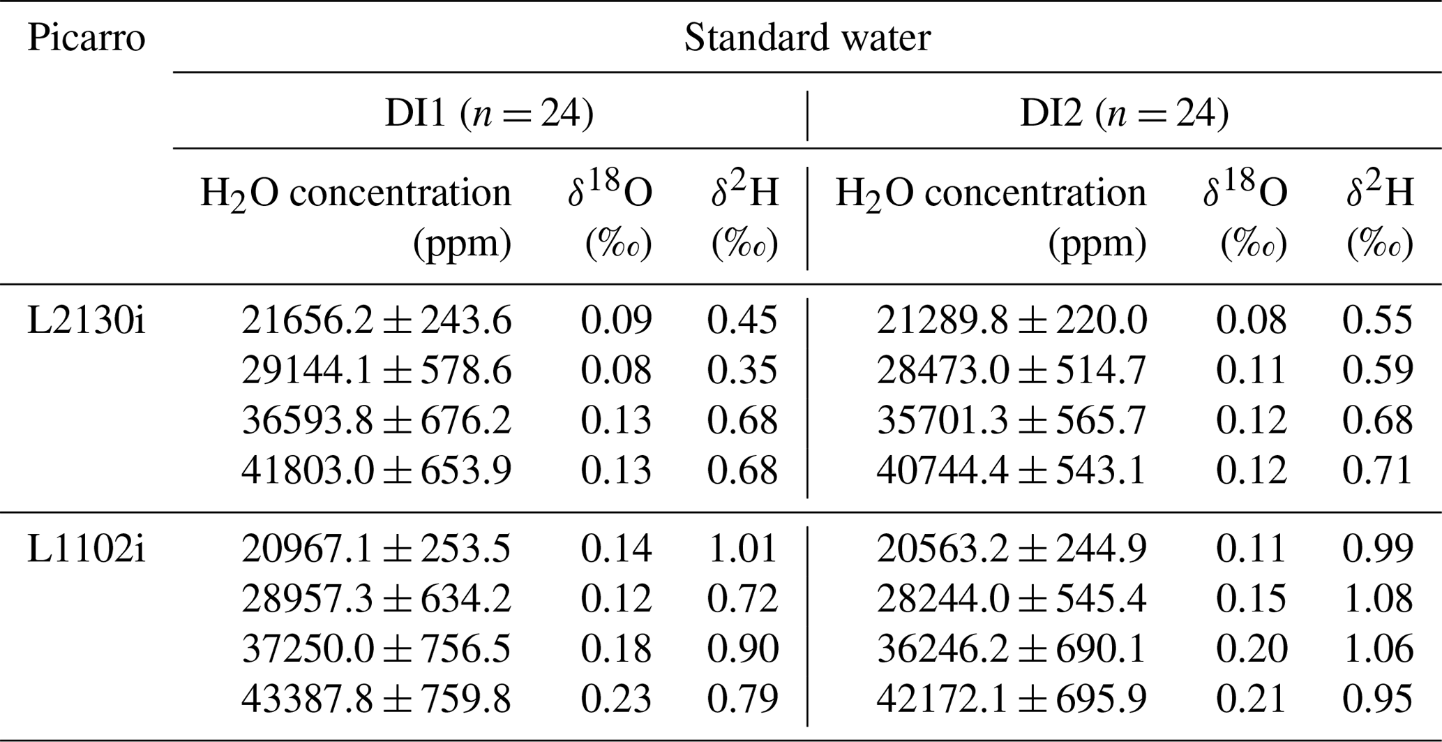
Table 1Standard deviations of δ18O and δ2H at each concentration level from all 24 calibration runs for the respective DI1 and DI2 standard waters. The standard deviations were calculated from the whole data set of raw 7 min average values, obtained by L2130i and L1102i on each calibration run. The mean values of H2O concentration at each concentration level were also calculated from all 24 data set of raw 7 min average values, obtained by L2130i and L1102i on each calibration run.
We also simulated regular automated calibration operation designed for field operations over the 2-week period to regularly supply the two CRDS analysers with standard water vapour samples at four different concentration levels from 21 500 to 41 000 ppm. We prepared two different working standard waters (DI1 and DI2) made of deionized water to avoid clogging the heated tubes and chamber inside the vaporizer unit with contaminants. Stable water isotope compositions (δ18O and δ2H) of the DI1 and DI2 standards were analysed at the MPI-BGC stable isotope laboratory (BGC-IsoLab) using isotope ratio mass spectrometry (IRMS). For details on the IRMS analysis, we refer readers to Gehre et al. (2004). The DI1 and DI2 standards were calibrated against VSMOW (Vienna Standard Mean Ocean Water) and SLAP (Standard Light Antarctic Precipitation) via in-house standards: DI1-δ18O = −25.07 ± 0.16 ‰, DI1-δ2H = −144.66 ± 0.60 ‰, DI2-δ18O = −3.69 ± 0.15 ‰, DI2-δ2H = −34.30 ± 1.00 ‰ (see also Sect. S1 in the Supplement). The isotopic span of the DI1 and DI2 almost covers the previously reported range of δ18O (−19.4 ‰ to −6.7 ‰) and δ2H (−151 ‰ to −42 ‰) for water vapour samples in the Ducke Reserve near Manaus or in Manaus, located near the ATTO site (Matsui et al., 1983; Moreira et al., 1997; IAEA/WMO, 2020). For calibration, we alternated between the two standard waters. One calibration run required 75 min, of which the first 30 min were used for stabilizing the produced standard water vapours at the highest concentration level and delivering them to the CRDS analysers. Subsequently the calibration system created stepwise lower concentration levels of the standard water vapour every 15 min by regulating the dilution flow rate. One calibration run consisted of a four-point concentration calibration at approximately 41 000, 36 000, 29 000, and 21 500 ppm. The actual measured mean and standard deviation of H2O concentration at the respective four concentration level for all the calibration cycles during the 2-week operation are shown in Table 1. The dilution flow rates for the different concentration levels were set to 9 sccm (41 000 ppm), 14 sccm (36 000 ppm), 21 sccm (29 000 ppm), and 28 sccm for 21 500 ppm. The set-point values were not changed during the 2-week test, thus simulating remote automatic on-site calibration runs. We used the last 7 min of data collected at each concentration level for the calibration assessment of the CRDS analysers. Immediately after a calibration cycle, the syringe pump drained the remaining standard water inside the tube between the vaporization chamber and the three-way solenoid valve 6 (SV6) through the waste line and then washed the inner space between the vaporization chamber and the SV1 valve three times with the standard water scheduled for the next calibration cycle (Fig. 1a and b). Subsequently, the rinsed vaporization chamber was fully dried with air from the dry-air unit for 2 to 4 h. These rinsing and drying steps were introduced to minimize the residual memory effect from the last calibration cycle on standard water vapour isotopic compositions during the next calibration run. We started the next calibration cycle 7 h after the start time of the last calibration cycle (i.e. the interval of the same working standard was 14 h). Throughout the entire experimental period, the calibration system conducted automatically 24 calibration runs for each standard water, which used 160 mL of each standard water in total.
We calculated isotopic deviations at each concentration level for each calibration cycle to evaluate [H2O] dependence of isotopic measurement accuracy. The isotopic deviations at each concentration level were obtained from the difference between measured isotopic values at each concentration level during each calibration cycle and assigned reference values at 21 500 ppm on each calibration run. We selected the 21 500 ppm level as the reference H2O condition because Picarro guarantees high δ18O and δ2H precision of CRDS analysers between 17 000–23 000 ppm of H2O and to make the results comparable with a similar past study (Tremoy et al., 2011) that assigned 20 000 ppm as the reference level. The assignment of reference values for each calibration cycle enabled us to assess isotopic biases that were mainly due to [H2O] dependence but not for other effects (e.g. drift effects on δ18O and δ2H accuracy between each calibration cycle).
2.3 Calibration for water vapour concentration dependence
We devised four strategies, referred to here as DI1, DI2, DI1–DI2*1Pair, and DI1–2*2Pairs, to use the automated calibration system to determine and correct for [H2O] dependence and used the 2-week operation to assess which calibration strategy decreased the uncertainties in δ18O and δ2H measurements the most. The DI1 and DI2 calibration strategies used a single standard water (DI1 or DI2) to correct for [H2O] dependence. In contrast, the DI1–DI2*1Pair and DI1–2*2Pairs strategies used the two standard waters (DI1 and DI2) for calibrating [H2O] dependence because we considered that [H2O] dependence might change between the two standard waters according to recent studies (Bonne et al., 2019; Weng et al., 2020). In addition, the DI1–2*2Pairs strategy used more calibration data than the DI1–DI2*1Pair strategy to obtain more robust calibration fittings of [H2O] dependence.
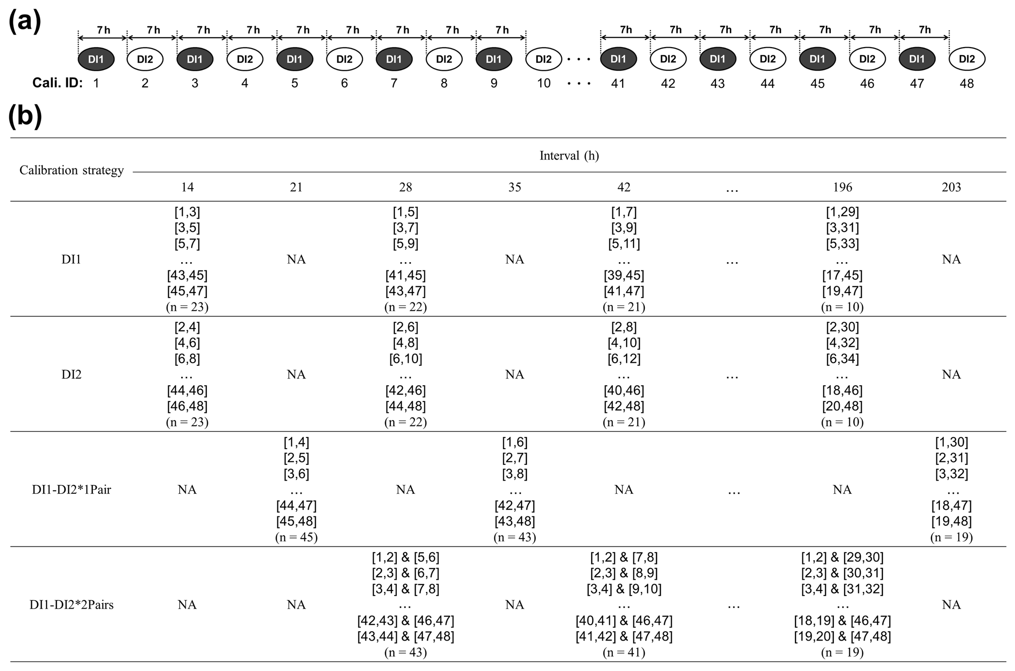
Figure 2Overview of the four different [H2O] dependence calibration strategies (DI1, DI2, DI1–DI2*1Pair, DI1–2*2Pairs) for assessing [H2O] dependence uncertainties of the L2130i and L1102i analysers related to the length of the calibration interval. (a) The top diagram shows a part of the total 48 calibration cycles, including both the DI1 and DI2 standard waters, with a 7 h interval and identity number (ID: 1–48) as an example. (b) The bottom table presents a part of which calibration cycles the four calibration strategies utilize for obtaining [H2O] dependence calibration fittings at different intervals as an example. The respective DI1 and DI2 strategies used a pair of only DI1 calibration cycles and a pair of only DI2 calibration cycles for obtaining calibration fittings of [H2O] dependence at intervals from 14 to 196 h. For example, the DI1 calibration strategy at a 14 h interval with ID-[1,3] used data sets from a pair of DI1 calibration cycles (ID-1 and ID-3) to obtain [H2O] dependence calibration fittings. The DI1–DI2*1Pair and DI1–2*2Pairs strategies used a pair of DI1 and DI2 calibration cycles, and two pairs of DI1 and DI2 calibration cycles, respectively, for obtaining calibration fittings of [H2O] dependence at intervals from 21 to 203 h (DI1–DI2*1Pair strategy) or from 28 to 196 h (DI1–DI2*2Pairs strategy). At each interval, the respective calibration strategy made all the pairs of each set calibration cycles (e.g. 43 two pairs at a 28 h interval for the DI1–DI2*2Pairs strategy) and then obtained calibration fittings from each pair of calibration cycles. For instance, as the DI1–DI2*2Pairs strategy utilized four two-dimensional (2D) fitting methods and one three-dimensional (3D) fitting method (i.e. linear, quadratic, cubic, quartic, and linear surface fitting methods) (see Sect. 2.3), the DI1–DI2*2Pairs strategy at a 28 h interval obtained 215 calibration fittings in total (i.e. 5 fitting methods × 43 two pairs) for the respective δ18O and δ2H accuracy. The procedure for assessing uncertainties in the obtained [H2O] dependence calibration fittings is described in Sect. 2.3.
Figure 2 summarizes the overview of the four calibration strategies. DI1 and DI2 refer to the two standard waters, measured at the four different concentration levels, and an identity number is assigned to the respective 48 calibration cycles (ID: 1–48), ordered by time during the experimental period (Fig. 2a). Hereinafter, we explain how to obtain calibration fittings and assess uncertainties of obtained calibration fittings by using the DI1–2*2Pairs strategy as an example. The DI1–2*2Pairs strategy uses two pairs of DI1 and DI2 calibration cycles (e.g. ID-[3,4] & [7,8] at a 28 h interval) for obtaining calibration fittings of [H2O] dependence at intervals from 28 to 196 h (Fig. 2b). The DI1–2*2Pairs strategy utilized four two-dimensional (2D) fitting methods and one three-dimensional (3D) fitting method (i.e. linear, quadratic, cubic, quartic, and linear surface fitting methods) to obtain [H2O] dependence calibration fitting parameters. For instance, the DI1–2*2Pairs strategy at a 28 h interval with ID-[3,4] & [7,8] obtained total 5 [H2O] dependence calibration fittings for each isotope accuracy.
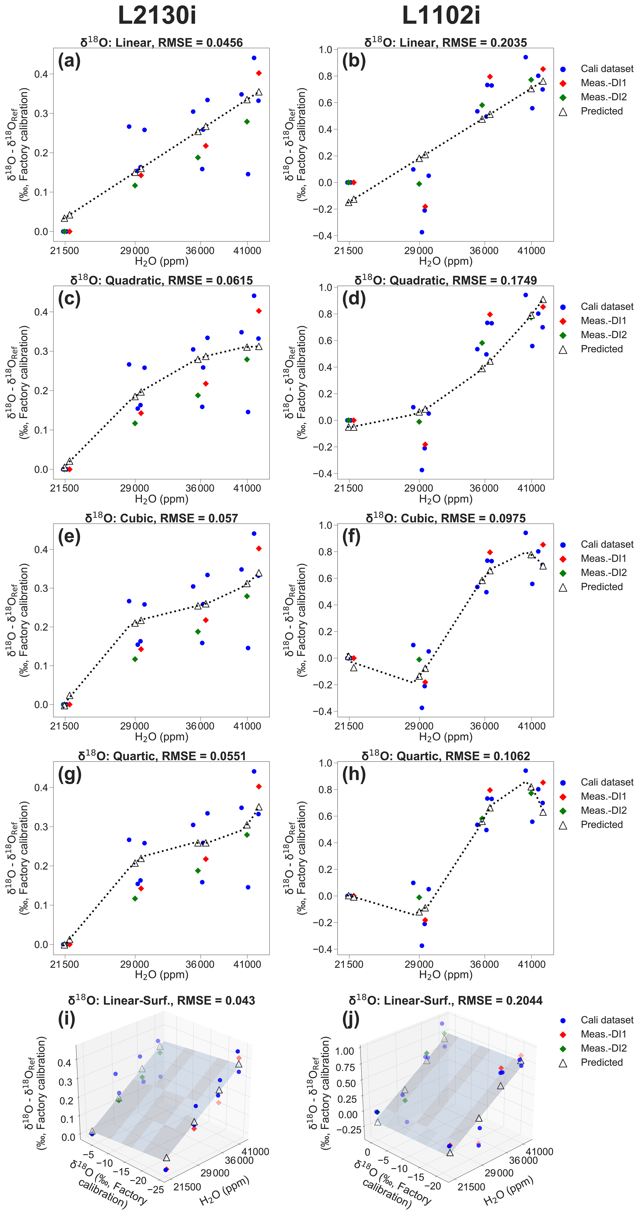
Figure 3Example of calibrating [H2O] dependence of δ18O accuracy for the respective L2130i and L1102i analysers by using four two-dimensional (2D) fitting methods and one three-dimensional (3D) fitting method (i.e. linear, quadratic, cubic, quartic, and linear surface fitting methods) according to the DI1–2*2Pairs calibration strategy at a 28 h interval with ID-[3,4] & [7,8] (see Fig. 2b). Calibrating (a) L2130i's and (b) L1102i's [H2O] dependence by using the linear fitting method. Calibrating (c) L2130i's and (d) L1102i's [H2O] dependence by using the quadratic fitting method. Calibrating (e) L2130i's and (f) L1102i's [H2O] dependence by using the cubic fitting method. Calibrating (g) L2130i's and (h) L1102i's [H2O] dependence by using the quartic fitting method. Calibrating (i) L2130i's and (j) L1102i's [H2O] dependence by using the linear surface fitting method. The blue dots on each plot represent data sets from two pairs of DI1 and DI2 calibration cycles (i.e. [3,4] & [7,8]) for obtaining each of the five calibration fittings. The respective 2D [H2O] dependence calibration fitting derives from a relationship between measured H2O concentration and δ18O deviation, equivalent to a difference between a measurement value of δ18O at each of the four concentration levels and that at the 21 500 ppm level (δ18ORef) on each calibration (a–h). The 3D [H2O] dependence calibration fitting also involves a measurement value of δ18O value at each concentration level as an independent variable (i–j). The red and green diamonds denote the actual observed δ18O deviations from unused DI1 (ID-5) and DI2 (ID-6) calibration cycles, respectively. The predicted δ18O deviations, denoted as open triangles, on each plot were calculated from each [H2O] dependence calibration fitting, applied to measured H2O concentrations (2D fitting methods; a–h) or to both measured H2O concentration and δ18O (3D fitting method; i–j) during the unused calibration cycles. The RMSE value on each plot was calculated from a difference between actual observed and predicted deviation values of δ18O.
As an example, Fig. 3 illustrates five calibration fittings for [H2O] dependence of δ18O accuracy for each CRDS analyser, acquired from two pairs of DI1 and DI2 calibration cycles (e.g. 3,4 and 7,8) following the DI1–2*2Pairs strategy at a 28 h interval (see also Fig. 2b). The respective 2D fitting is acquired from a relationship between H2O concentrations, measured at four different levels, and δ18O deviation at each of the four-point levels (the blue dots in Fig. 3a–h). The linear surface fitting also involves measuring the δ18O value at each concentration level as an independent variable (Fig. 3i and j). The procedure for calculating isotopic deviations at each concentration level was the same as described in Sect. 2.2.
The quantitative evaluation of uncertainties in [H2O] dependence calibration was conducted by means of root mean square error (RMSE) between actual observed and predicted isotopic deviation values by obtained [H2O] dependence fittings. We calculated the RMSE value for each of the [H2O] dependence 2D or 3D fittings as follows:
where δ(obs) is the actual observed deviation value of δ18O or δ2H at each concentration level from measurement cycles, δ(pred) is the predicted deviation value of δ18O or δ2H at each concentration level, and n is the sample number. The measurement cycles represent calibration cycles that were not used for estimating [H2O] dependence, over an interval period between one or two calibration pairs. For example, in the case of the DI1–2*2Pairs strategy at a 28 h interval with ID-[3,4] & [7,8], DI1 (ID-5) and D2 (ID-6) calibration cycles are regarded as measurement cycles (Fig. 2). The measured δ18O deviation value at each concentration level during the measurement cycles (e.g. red dots: DI1, ID-5; green dots: DI2, ID-6; Fig. 3) represents the value of δ(obs) at each concentration level. The predicted isotopic deviation value (δ(pred)) at each concentration level during the measurement cycles (e.g. DI1: 5, DI2: 6) is calculated by each of the [H2O] dependence 2D or 3D fittings, applied to the measured value of H2O concentration at each concentration level (the open triangles in Fig. 3a–h) or to the measured values of both H2O concentration and δ18O at each concentration level during the measurement cycles (the open triangles in Fig. 3i and j). The example of calculated δ18O RMSE of each fitting method for each CRDS analyser is shown on each plot in Fig. 3.
We conducted δ18O and δ2H RMSE evaluation for all the [H2O] dependence fittings that were obtained from all the respective two pairs of DI1 and DI2 calibration cycles at each interval period (28–196 h) following the DI1–2*2Pairs strategy over the entire 2-week period (see Fig. 2b). For instance, since the DI1–2*2Pairs strategy at a 28 h interval formed 43 two pairs in total (i.e. [1,2] & [5,6], [2,3] & [6,7], [3,4] & [7,8], …, [42,43] & [46,47], [43,44] & [47,48]) (see Fig. 2b), we calculated δ18O and δ2H RMSE values for each of the 43 [H2O] dependence linear, quadratic, cubic, quartic, or linear surface fittings.
Compared with the DI1–2*2Pairs strategy, the DI1, DI2, and DI1–DI2*1Pair calibration strategies used a pair of only DI1 calibrations, a pair of only DI2 calibrations, and a pair of DI1 and DI2 calibrations, respectively, for acquiring [H2O] dependence fittings at intervals from 14 to 196 h (DI1, DI2 calibration strategies) or from 21 to 203 h (DI1–DI2*1Pair calibration strategy) (Fig. 2b). The DI1 and DI2 calibration strategies utilized the four 2D fitting methods for obtaining [H2O] dependence calibration fittings, whereas the DI1–DI2*1Pair calibration strategy used the four 2D and one 3D fitting methods as with the DI1–2*2Pairs strategy. For each calibration strategy, we also calculated the RMSE value for each of the [H2O] dependence 2D or 3D fittings.
3.1 Measurement precision over the 2-week period
Figure 4 shows example times series of 7 min mean H2O concentration, δ18O, and δ2H, calculated from raw L2130i measurement data for the highest and lowest H2O concentrations (i.e. ∼ 41 000 and ∼ 21 500 ppm) over the entire DI1 standard water calibration runs for the 2-week period. The precision is defined as the standard deviation (σ) of all the raw 7 min average values over the 24 calibrations. The temporal changes in measured H2O concentration at 21 500 ppm varied with H2O σ = 243.6 ppm (1.1 %) over the whole period, whereas the highest moisture condition (∼ 41 000 ppm) had larger variation of H2O concentration (H2O σ: 653.9 ppm or ∼ 1.5 %; Fig. 4a and b). The larger variability at 41 000 ppm likely derived from difficulty in establishing and delivering a stable high moisture stream from the calibration unit to L2130i and possibly residual memory effects inside the tube line and L2130's measurement cell even with the well-heated condition (cell temperature = 80 ∘C) due to the extremely high moisture. One solution of the possible residual memory effects would be an increase in the tube heater's temperature above 45 ∘C. In addition, the larger variation in H2O concentration at 41 000 ppm may have been influenced by the instability of the calibration system and a saturation effect inside the cavity measuring H2O concentration near the upper limit (50 000 ppm). Moreover, the less stable H2O signal at the highest concentration level results in lower precisions of δ18O (σ = 0.13 ‰) and δ2H (σ = 0.68 ‰) compared with at the lowest concentration level (δ18O σ = 0.09 ‰ and δ2H σ = 0.45 ‰) (Fig. 4c–f).
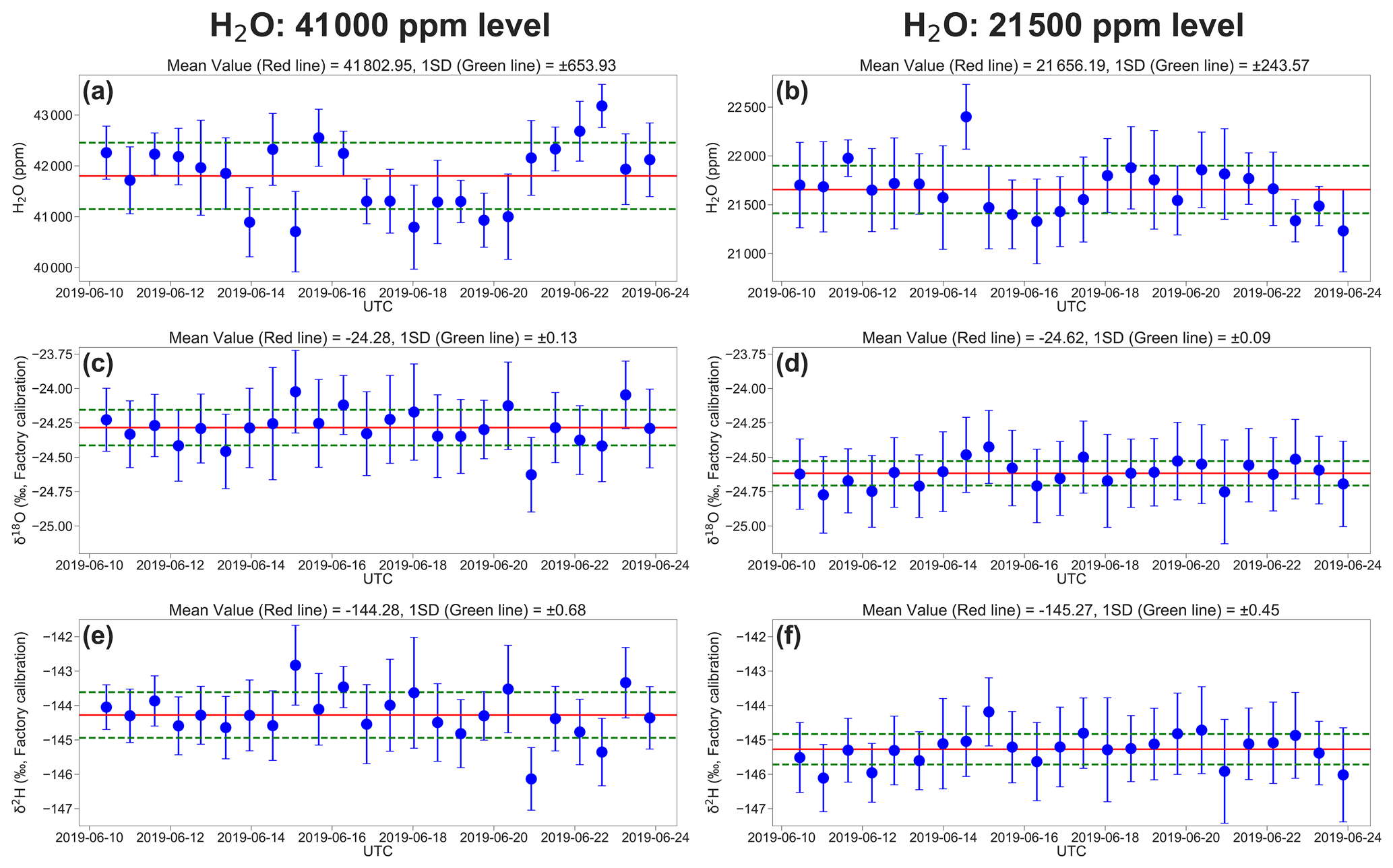
Figure 4The 2-week evolution of the L2130i's measurements for the DI1 standard water in (a) H2O concentration at the 41 000 ppm level, (b) H2O concentration at the 21 500 ppm level, (c) δ18O at the 41 000 ppm level, (d) δ18O at the 21 500 ppm level, (e) δ2H at the 41 000 ppm level, and (f) δ2H at the 21 500 ppm level. Each value is a 7 min average of raw measurement data from the L2130i, and error bars are 1 standard deviation of 7 min. The red and green lines show the average and standard deviation through the 2-week measurement period.
Table 1 summarizes the precision of δ18O and δ2H for each concentration level for each standard water for the L2130i and L1102i analysers. For both standard waters, the L2130i analyser had higher δ18O and δ2H precision than the L1102i analyser, likely due to the improved fitting algorithm used for the L2130i analyser (Aemisegger et al., 2012). In addition, the L2130i analyser had higher δ18O (σ ≤ 0.11 ‰) and δ2H (σ ≤ 0.59 ‰) precision under 30 000 ppm than over 30 000 ppm: δ18O σ ≥ 0.12 ‰ and δ2H σ ≥ 0.68 ‰ (Table 1). The L1102i analyser also had higher precision below 30 000 ppm relative to over 30 000 ppm except δ2H precision for DI2 (Table 1). These findings indicate that both analysers can measure stable water isotopes more precisely for water vapour samples below 30 000 ppm.
Across concentration levels for DI2, both analysers had the highest δ18O and δ2H measurement precision at the 21 500 ppm level with the lowest H2O variation (H2O σ ≤ 244.9 ppm) except δ2H precision of L1102i. In contrast, for DI1, both analysers had the highest δ18O and δ2H measurement precision at 29 000 ppm, even though variability in H2O concentration measurement was higher at 29 000 ppm (H2O σ ≥ 578.6 ppm) than at 21 500 ppm (H2O σ ≤ 253.5 ppm). The high measurement precision of L2130i and L1102i even with the larger H2O concentration variability indicates that the measurement precision of the L2130i and L1102i analysers was not largely influenced by the instability of the calibration unit. Furthermore, the L1102i's δ18O and δ2H values of precision at 21 500 ppm (δ18O σ = 0.11 ‰–0.14 ‰ and δ2H σ = 0.99 ‰–1.01 ‰) were similar or better than those reported by Delattre et al. (2015) at 20 000 ppm for the L1102i (δ18O and δ2H precision of 0.08 ‰–0.19 ‰ and 1.5 ‰–2.0 ‰ respectively, based on 40 calibration data over 35 d). This proves that the calibration system has a negligible effect on the isotopic measurement precision for L2130i and L1102i analysers.
3.2 Accuracy of isotope values for water vapour concentration dependence
For the L2130i analyser, the δ18O deviation of both standard waters from reference values at 21 500 ppm gradually increased with H2O concentration, reaching a maximum median value of 0.32 ‰ for DI1 and of 0.28 ‰ for DI2 (Fig. 5a). For δ18O, these differences were significant for both standard waters between 41 000 and 36 000 or 29 000 ppm (Fig. 5a; Welch's t test, p < 0.01), but differences between 36 000 and 29 000 ppm were not significant (Fig. 5a; Welch's t test, p > 0.09). As with δ18O, the values of δ2H measured with the L2130i for both standard waters differed significantly between 41 000 ppm and the lower H2O concentrations (Fig. 5b; Welch's t test, p < 0.05), without a significant difference between 29 000 and 36 000 ppm (Fig. 5b; Welch's t test, p > 0.86). These results indicate that accurate measurement of both δ18O and δ2H using the L2130i analyser require correction for [H2O] dependence under high moisture conditions (> 36 000 ppm H2O).
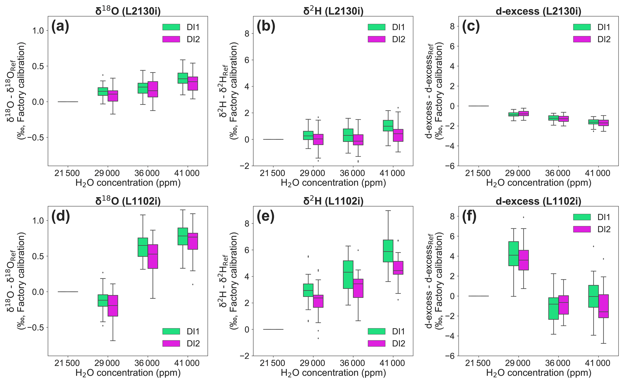
Figure 5Deviations of stable isotopic compositions (δ18O, δ2H, and d-excess) for each standard water (DI1 and DI2) at three different H2O concentrations compared to the 21 500 reference H2O concentration. Box plots of (a) δ18O, (b) δ2H, and (c) d-excess deviations, measured by L2130i. Box plots of (d) δ18O, (e) δ2H, and (f) d-excess deviations, measured by L1102i. The δ18O, δ2H, and d-excess values at 21 500 ppm are assigned a value of 0, and [H2O] dependence for each isotope can be observed as the deviation between the value at each concentration level from the value measured at 21 500 ppm.
The differences in the L2130i's deviation of each isotope from reference values at 21 500 ppm were similar for the two standard waters at all concentration levels except 41 000 ppm (Fig. 5a and b, Welch's t test, p > 0.05), where the L2130i indicated differences in δ2H deviation for the two different standard waters (Fig. 5b; Welch's t test, p < 0.05). This finding indicates that the L2130i's δ2H accuracy for high moisture like 41 000 ppm is dependent on the isotopic composition, such as has been found for low moisture conditions below 4000 ppm (Weng et al., 2020). This result further indicates that more than one standard water needs to be used in the field under not only low moisture, but also high moisture conditions. Additionally, the isotope dependence of δ2H accuracy may have been related to the low suction flow rate of the L2130i (Thurnherr et al., 2020).
The [H2O] dependence of δ18O and δ2H accuracy also gives rise to uncertainty in deuterium excess (hereinafter called d-excess; d-excess = δ2H–8δ18O) values, estimated with the uncorrected δ18O and δ2H values (Fig. 5c and f). The d-excess deviation of the L2130i analyser significantly increased in a negative direction with concentration level for each standard water and reached a maximum negative median value of −1.62 ‰ for DI1 and of −1.70 ‰ for DI2 (Fig. 5c). According to the calculation of d-excess, the decrease in d-excess with H2O concentration mostly stemmed from the increase in the L2130i's δ18O values with H2O concentration (Fig. 5a and c), which underlines the need for correcting for the [H2O] dependence, especially for δ18O accuracy at high concentration levels using the L2130i analyser.
The L1102i also had strong [H2O] dependence for both isotopes, larger than that of the L2130i (Fig. 5a–b and d–e). The larger variations also led to large deviations in the d-excess values (Fig. 5f). In addition, both δ18O and δ2H accuracy for the L1102i depend on isotopic compositions (δ18O: 36 000 ppm, δ2H: all concentration levels; Fig. 5d and e, Welch's t test, p < 0.05), different from the L2130i analyser. The above findings indicate that for the L1102i both δ2H and δ18O accuracy depend on H2O concentration and the isotopic compositions, thus making the [H2O] dependence correction for both the δ2H and δ18O accuracy using different standard waters necessary.
The L1102i's results of δ18O and δ2H deviations were comparable with those reported by Tremoy et al. (2011), who tested [H2O] dependence on δ18O and δ2H accuracy for L1102i of up to 39 000 ppm against the reference H2O concentration at 20 000 ppm. However, Tremoy et al. (2011) observed negative δ18O deviations at 39 000 ppm with a range between −2 ‰ and 0 ‰, different from this study. In addition, they showed a smaller increase in δ2H deviations with H2O concentration from 20 000 to 39 000 ppm than this study. The above differences in δ18O and δ2H deviations between Tremoy et al. (2011) and this study show that [H2O] dependence of δ18O and δ2H accuracy must be evaluated for each individual analyser (Aemisegger et al., 2012; Bailey et al., 2015).
In summary, the measurement accuracy of δ18O and δ2H is more dependent on H2O concentration for the L1102i than the L2130i, likely due to the older fitting algorithm for the initial version of the L1102i. In other words, the accuracy of [H2O] dependence of δ18O and δ2H for the L2130i has been improved due to the updated/corrected fitting algorithm (Aemisegger et al., 2012), but our results still remind us of the importance of correcting for the [H2O] dependence of δ18O and δ2H accuracy for the L2130i analyser, particularly for high moisture conditions at 36 000 ppm and above.
3.3 Strategy for calibration of isotope values for water vapour concentration dependence
The four calibration strategies for correcting isotope values using measured H2O concentrations are compared in Fig. 6. Across methods, the L2130i analyser usually displays lower median δ18O RMSE values compared to the L1102i analyser (Fig. 6). This tendency is also found in δ2H RMSE results for each calibration strategy (see Fig. S1 in the Supplement). The lower RMSE values of the L2130i analyser are mainly due to the higher precision of the L2130i analyser compared to the L1102i analyser.
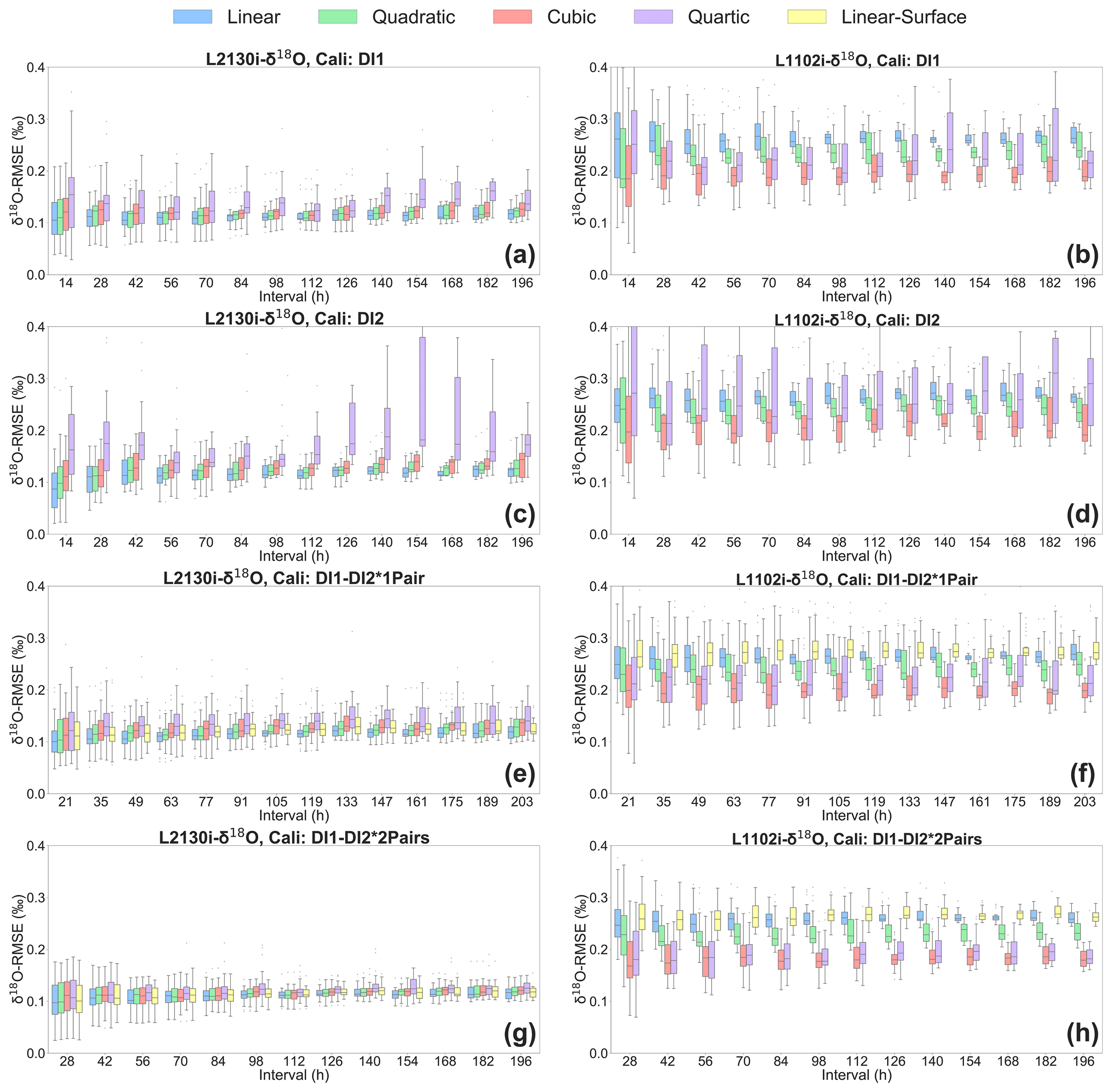
Figure 6Box plots of root mean square error (RMSE) of δ18O, derived from calibrating [H2O] dependence of δ18O measurements by each of the five fitting methods (i.e. linear, quadratic, cubic, quartic, and linear surface fitting methods) for each of the four calibration strategies: DI1, DI2, DI1–DI2*1Pair, DI1–2*2Pairs. Box plots of (a) L2130's and (b) L1102's δ18O RMSE for the DI1 strategy, depending on interval length (i.e. the time period used for calibrating [H2O] dependence). Box plots of (c) L2130's and (d) L1102's δ18O RMSE for the DI2 strategy, depending on interval length. Box plots of (e) L2130's and (f) L1102's δ18O RMSE for the DI1–DI2*1Pair strategy, depending on interval length. Box plots of (g) L2130's and (h) L1102's δ18O RMSE for the DI1–2*2Pairs strategy, depending on interval length. The procedure for assessing [H2O] dependence uncertainties (RMSE) is described in Sect. 2.3.
The lowest median RMSE for the L1102i analyser is the cubic fitting method (Fig. 6b, d, f and h). Among all the calibration strategies of the L1102i analyser, the DI1–2*2Pairs calibration strategy with the cubic fitting method usually shows the minimum median RMSE value for δ18O accuracy (Fig. 6h). For δ2H accuracy of the L1102i analyser, the DI1–2*2Pairs calibration strategy also usually displays lower median RMSE values relative to the other strategies. These results indicate that this calibration strategy is most appropriate for correcting [H2O] dependence and improving the accuracy of isotope measurements with the L1102i analyser.
Compared with the L1102i analyser, the DI1–2*2Pairs calibration strategy of the L2130i analyser does not show clearly reduced isotopic RMSE values relative to the other calibration strategies but still displays low RMSE values with a small distribution from each fitting method at each interval (Figs. 6a, c, e, g and S1). This indicates that the DI1–2*2Pairs strategy can be utilized for correcting [H2O] dependence of the L2130i analyser as well as the L1102i analyser. Since the calibration system uses the same tube line between the vaporizer and the branch point before the inlet port of each CRDS analysers (Fig. 1a), we decided to utilize the DI1–2*2Pairs strategy for the L2130i analyser in the same way as the L1102i analyser.
Each CRDS analyser using the DI1–2*2Pairs strategy shows the lowest median RMSE values of isotopic accuracy at the shortest interval (28 h), which only slightly increases with intervals over 8 d (Fig. 6g and h). This indicates that one [H2O] dependence calibration per week is enough to maintain good isotopic measurement of the CRDS analysers for an in situ continuous observation remotely. According to the recent studies (Bonne et al., 2019; Weng et al., 2020), new CRDS models (e.g. L2130i and L2140i) did not show any significant changes for [H2O] dependence from ∼ 500 to 25 000 ppm over several months up to 2 years. The consistency of [H2O] dependence may be extended to higher moisture conditions than 25 000 ppm, but based on our laboratory experiments, we decided to conduct the [H2O] dependence calibration at intervals of 1 week or less with the DI1–2*2Pairs strategy. After we continuously run the ambient measurement and calibration systems at the ATTO site over several months, we will try to reduce the [H2O] dependence calibration frequency to maximize the ambient sampling period while maintaining high measurement accuracy of both CRDS analysers.
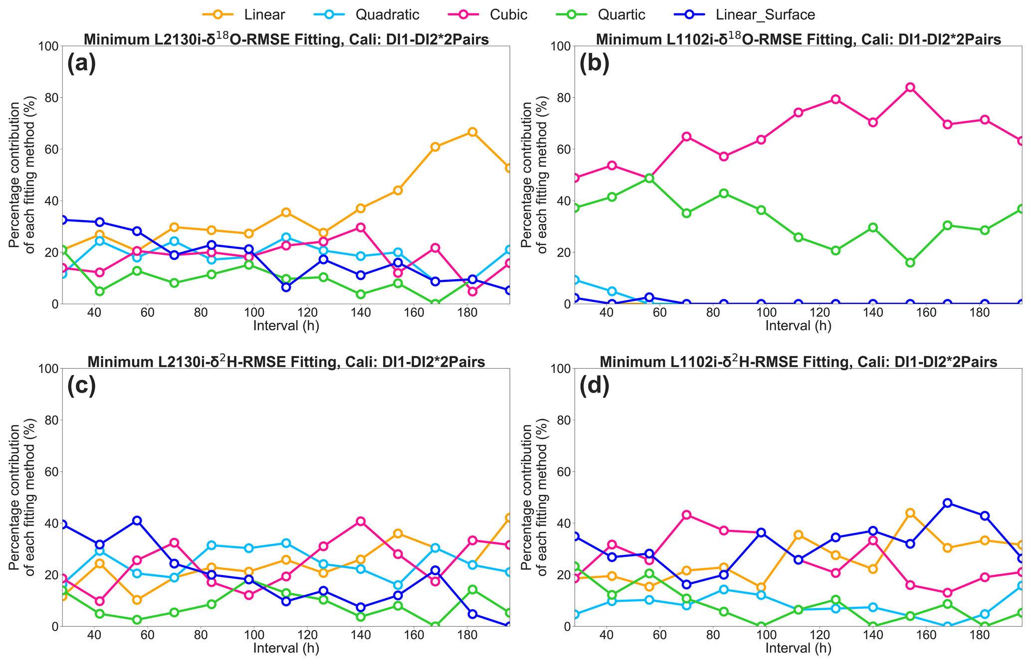
Figure 7Percentage contribution of the respective five [H2O] dependence fittings (i.e. linear, quadratic, cubic, quartic, and linear surface fitting methods) to the total calibration pairs, which only obtained minimum RMSE values of δ18O and δ2H, at each interval for the DI1–2*2Pairs calibration strategy. (a) L2130i's and (b) L1102i's results for δ18O RMSE. (c) L2130i's and (d) L1102i's results for δ2H RMSE.
For both analysers using the DI1–2*2Pairs strategy, the RMSE distribution of isotopic accuracy gradually gets smaller with intervals over 8 d (Fig. 6g and h). The smaller RMSE distributions at long intervals result from larger sample numbers for calculating RMSE values at long intervals, whereas the larger RMSE distributions at short intervals are attributed to smaller sample numbers for calculating RMSE (e.g. 28 h with ID-[3,4] & [7,8]: n = 8 (4 samples × 2 measurement cycles, i.e. ID-5,6), 196 h with ID-[3,4] & [31,32]: n = 104 (4 samples × 26 measurement cycles, i.e. ID-5-30); see Fig. 2b).
The respective CRDS analyser with the DI1–2*2Pairs strategy also shows a similar range of RMSE among the five curve-fitting methods (Figs. 6g–h and S1g–h). The results do not clearly indicate which fitting method most frequently obtains the lowest RMSE values for each [H2O] dependence calibration interval. Hence, for the DI1–2*2Pairs strategy we obtained a [H2O] dependence fitting method, which only obtained minimum RMSE values of δ18O and δ2H, from each two calibration pairs at each interval, and then calculated a contribution rate of the respective five [H2O] dependence fittings (i.e. linear, quadratic, cubic, quartic, and linear surface fitting methods) to the total calibration pairs at each interval (Fig. 7). The linear surface fitting method most frequently gives the lowest isotopic RMSE values, except δ18O accuracy of the L1102i analyser (i.e. cubic fitting method), at a 28 h interval (Fig. 7). This indicates that the linear surface fitting method at a 28 h interval reduces uncertainties in correcting [H2O] dependence on isotopic accuracy most effectively, except for δ18O accuracy of the L1102i analyser. Compared with the 28 h interval, the 2D fitting methods are the most appropriate for calibrating [H2O] dependence on isotopic accuracy over long intervals, excluding δ2H accuracy of the L1102i analyser (Fig. 7). The difference in fitting methods between 28 h and longer intervals suggests that the 28 h interval strategy can correct for both [H2O]- and isotope-dependent errors by using the 3D fitting method, whereas the strategies using long intervals can correct for only [H2O]-dependent errors with the 2D fitting methods.
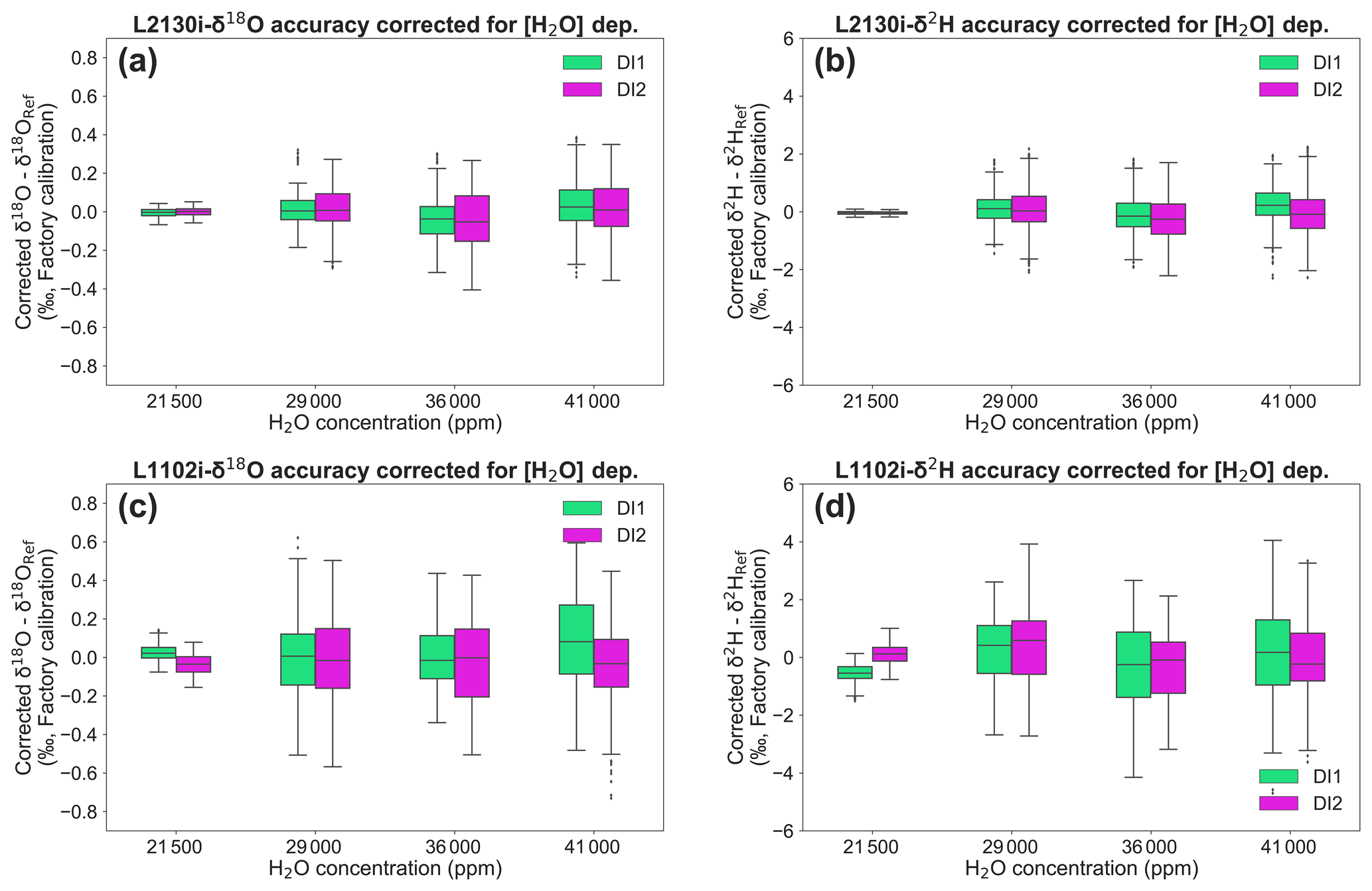
Figure 8Deviations of δ18O and δ2H, both corrected for [H2O] dependence, for each standard water (DI1 and DI2) at four different H2O concentrations. Box plots of (a) δ18O and (b) δ2H deviations, corrected for [H2O] dependence of L2130i. Box plots of (c) δ18O and (d) δ2H deviations, corrected for [H2O] dependence of L1102i. The [H2O] dependence of each CRDS analysers was corrected by the DI1–2*2Pairs calibration strategy with the best fitting methods (L2130i-δ18O: linear fitting, L2130i-δ2H: quadratic fitting, L1102i-δ18O: cubic fitting, L1102i-δ2H: linear surface fitting) at a 168 h interval.
Figure 8 presents the corrected isotope deviations by the best fitting methods (L2130i-δ18O: linear fitting, L2130i-δ2H: quadratic fitting, L1102i-δ18O: cubic fitting, L1102i-δ2H: linear surface fitting) at a weekly (i.e. 168 h) interval by assuming the continuous operation at the ATTO site, discussed above. The isotope deviations of each CRDS analysers do not substantially vary with H2O concentration. This indicates that the calibrations successfully corrected [H2O] dependence of isotope accuracy for each analyser. Based on Moreira et al. (1997), water vapour isotope values in the Amazon rainforest is expected to change diurnally by up to 2 ‰ (δ18O) or 4 ‰–8 ‰ (δ2H) with H2O concentration. The diel isotope variations are higher than the corrected deviation values of each CRDS analyser (Fig. 8). This supports the finding that both the CRDS analysers will detect diel or probably seasonal/interannual variations in water vapour isotopes in the Amazon rainforest.
This study extends previous work documenting water vapour concentration dependence of Picarro CRDS analysers on high moisture (> 35 000 ppm H2O), likely to be measured in the Amazon rainforest and other tropical areas. We assessed the precision and accuracy of two CRDS analysers (i.e. model L1102i and L2130i) for concentration and isotopic measurements by using a custom-made calibration unit that regularly supplied standard water vapour samples at four different H2O concentrations between 21 500 and 41 000 ppm to the CRDS analysers. Our results demonstrate that the newer version of the analyser (L2130i) has better precision for both δ18O and δ2H measurements under all H2O concentration levels compared to the older model (L1102i). In addition, isotope measurements in both analysers varied with H2O concentration, especially at H2O concentration over 36 000 ppm. The concentration dependence of the L1102i analyser was stronger than the L2130i analyser. These findings indicate that calibrating the [H2O] dependence of δ18O and δ2H measurements for both the CRDS analysers during field deployment in high atmospheric moisture areas such as tropical forests is important.
Assuming continuous in situ observations together with regular calibration in the tropical Amazon rainforest, we devised four calibration strategies, adjusted to our custom-made calibration system, and then evaluated which [H2O] dependence calibration procedure best improved the accuracy of δ18O and δ2H measurements for both the L2130i and L1102i analysers. The best [H2O] dependence strategy was the DI1–2*2Pairs strategy that required two pairs of a two-point calibration with different concentration levels from 21 500 to 41 000 ppm. The 28 h interval strategy with the linear surface fitting method leads to the most accurate measurements for both the CRDS analysers, except δ18O accuracy of the L1102i analyser that required the cubic fitting method. In addition, [H2O] dependence calibration uncertainties hardly changed at any interval over 8 d. That indicates one [H2O] dependence calibration per week is sufficient for correcting moisture-biased isotopic accuracy of the CRDS analysers. The best calibration strategy at a weekly interval also supported the finding that both CRDS analysers can sufficiently distinguish temporal variations of water vapour isotopes at the study site, ATTO. In addition, since the recent studies indicate the consistency of the [H2O] dependence for the CRDS analysers over several months up to 2 years, we intend to determine the appropriate frequency for calibrating [H2O] dependence under high moisture conditions after a continuous operation over several months at the ATTO site to maximize the ambient sampling period.
All the data used in this publication are freely available at https://doi.org/10.17617/3.4n (Komiya and Lavric, 2020).
The supplement related to this article is available online at: https://doi.org/10.5194/amt-14-1439-2021-supplement.
The calibration system was designed and developed by SK, JVL, TS, and US. The laboratory experiments were conducted by SK with assistance from JVL, TS, US, and FK. The IRMS analysis was done by HM and HG. DW helped us to check water vapour concentration at the ATTO site. SK conducted the data analysis and wrote the manuscript with assistance from JVL, FK, and HM. SK wrote the manuscript with contributions from all co-authors.
The authors declare that they have no conflict of interest.
We are grateful to Susan Trumbore (MPI-BGC) for reviewing the earlier manuscript and for her valuable feedback, to Stefan Wolff and Matthias Sörgel (MPI-Chemistry) for helping us to check H2O concentration at the ATTO site, and also to Jürgen M. Richter (MPI-BGC) for helping us to prepare the DI1 and DI2 standard waters.
This research has been supported by the Max Planck Society and the German Federal Ministry of Education and Research (BMBF; grant no. 01LK1602A).
The article processing charges for this open-access
publication were covered by the Max Planck Society.
This paper was edited by Thomas F. Hanisco and reviewed by two anonymous referees.
Aemisegger, F., Sturm, P., Graf, P., Sodemann, H., Pfahl, S., Knohl, A., and Wernli, H.: Measuring variations of δ18O and δ2H in atmospheric water vapour using two commercial laser-based spectrometers: an instrument characterisation study, Atmos. Meas. Tech., 5, 1491–1511, https://doi.org/10.5194/amt-5-1491-2012, 2012.
Aemisegger, F., Vogel, R., Graf, P., Dahinden, F., Villiger, L., Jansen, F., Bony, S., Stevens, B., and Wernli, H.: How Rossby wave breaking modulates the water cycle in the North Atlantic trade wind region, Weather Clim. Dynam. Discuss. [preprint], https://doi.org/10.5194/wcd-2020-51, in review, 2020.
Andreae, M. O., Acevedo, O. C., Araùjo, A., Artaxo, P., Barbosa, C. G. G., Barbosa, H. M. J., Brito, J., Carbone, S., Chi, X., Cintra, B. B. L., da Silva, N. F., Dias, N. L., Dias-Júnior, C. Q., Ditas, F., Ditz, R., Godoi, A. F. L., Godoi, R. H. M., Heimann, M., Hoffmann, T., Kesselmeier, J., Könemann, T., Krüger, M. L., Lavric, J. V., Manzi, A. O., Lopes, A. P., Martins, D. L., Mikhailov, E. F., Moran-Zuloaga, D., Nelson, B. W., Nölscher, A. C., Santos Nogueira, D., Piedade, M. T. F., Pöhlker, C., Pöschl, U., Quesada, C. A., Rizzo, L. V., Ro, C.-U., Ruckteschler, N., Sá, L. D. A., de Oliveira Sá, M., Sales, C. B., dos Santos, R. M. N., Saturno, J., Schöngart, J., Sörgel, M., de Souza, C. M., de Souza, R. A. F., Su, H., Targhetta, N., Tóta, J., Trebs, I., Trumbore, S., van Eijck, A., Walter, D., Wang, Z., Weber, B., Williams, J., Winderlich, J., Wittmann, F., Wolff, S., and Yáñez-Serrano, A. M.: The Amazon Tall Tower Observatory (ATTO): overview of pilot measurements on ecosystem ecology, meteorology, trace gases, and aerosols, Atmos. Chem. Phys., 15, 10723–10776, https://doi.org/10.5194/acp-15-10723-2015, 2015.
Bailey, A., Toohey, D., and Noone, D.: Characterizing moisture exchange between the Hawaiian convective boundary layer and free troposphere using stable isotopes in water, J. Geophys. Res.-Atmos., 118, 8208–8221, https://doi.org/10.1002/jgrd.50639, 2013.
Bailey, A., Noone, D., Berkelhammer, M., Steen-Larsen, H. C., and Sato, P.: The stability and calibration of water vapor isotope ratio measurements during long-term deployments, Atmos. Meas. Tech., 8, 4521–4538, https://doi.org/10.5194/amt-8-4521-2015, 2015.
Bindoff, N. L., Stott, P. A., AchutaRao, K. M., Allen, M. R., Gillett, N., Gutzler, D., Hansingo, K., Hegerl, G., Hu, Y., Jain, S., Mokhov, I. I., Overland, J., Perlwitz, J., Sebbari, R., and Zhang, X.: Detection and attribution of climate change: from global to regional, Climate Change 2013: The Physical Science Basis, Contribution of Working Group I to the Fifth Assessment Report of the Intergovernmental Panel on Climate Change, edited by: Stocker, T. F., Qin, D., Plattner, G.-K., Tignor, M., Allen, S. K., Boschung, J., Nauels, A., Xia, Y., Bex, V., and Midgley, P. M., Cambridge University Press, Cambridge, UK and New York, NY, USA, 2013.
Bonne, J.-L., Behrens, M., Meyer, H., Kipfstuhl, S., Rabe, B., Schönicke, L., Steen-Larsen, H. C., and Werner, M.: Resolving the controls of water vapour isotopes in the Atlantic sector, Nat. Commun., 10, 1632, https://doi.org/10.1038/s41467-019-09242-6, 2019.
Coe, M. T., Macedo, M. N., Brando, P. M., Lefebvre, P., Panday, P., and Silvério, D.: The Hydrology and Energy Balance of the Amazon Basin, in: Interactions Between Biosphere, Atmosphere and Human Land Use in the Amazon Basin, edited by: Nagy, L., Forsberg, B. R., and Artaxo, P., Springer, Berlin, Heidelberg, Germany, 35–53, 2016.
Craig, H. and Gordon, L.: Deuterium and oxygen 18 variations in the ocean and the marine atmosphere, in: Stable Isotopes in Oceanographic Studies and Paleotemperatures, edited by: Tongiorgi, E., Stable Isotopes in Oceanographic Studies and Paleotemperatures, Spoleto, Italy, Laboratorio di Geologica Nucleare, Pisa, Italy, 9–130, 1965.
Dansgaard, W.: Stable isotopes in precipitation, Tellus, 16, 436–468, https://doi.org/10.1111/j.2153-3490.1964.tb00181.x, 1964.
Delattre, H., Vallet-Coulomb, C., and Sonzogni, C.: Deuterium excess in the atmospheric water vapour of a Mediterranean coastal wetland: regional vs. local signatures, Atmos. Chem. Phys., 15, 10167–10181, https://doi.org/10.5194/acp-15-10167-2015, 2015.
Galewsky, J., Steen-Larsen, H. C., Field, R. D., Worden, J., Risi, C., and Schneider, M.: Stable isotopes in atmospheric water vapor and applications to the hydrologic cycle: Isotopes in the Atmospheric Water Cycle, Rev. Geophys., 54, 809–865, https://doi.org/10.1002/2015rg000512, 2016.
Gehre, M., Geilmann, H., Richter, J., Werner, R. A., and Brand, W. A.: Continuous flow 2H/1H and 18O/16O analysis of water samples with dual inlet precision, Rapid Commun. Mass Sp., 18, 2650–2660, https://doi.org/10.1002/rcm.1672, 2004.
González, Y., Schneider, M., Dyroff, C., Rodríguez, S., Christner, E., García, O. E., Cuevas, E., Bustos, J. J., Ramos, R., Guirado-Fuentes, C., Barthlott, S., Wiegele, A., and Sepúlveda, E.: Detecting moisture transport pathways to the subtropical North Atlantic free troposphere using paired H2O-δD in situ measurements, Atmos. Chem. Phys., 16, 4251–4269, https://doi.org/10.5194/acp-16-4251-2016, 2016.
Helliker, B. R. and Noone, D.: Novel Approaches for Monitoring of Water Vapor Isotope Ratios: Plants, Lasers and Satellites, in: Isoscapes: Understanding movement, pattern, and process on Earth through isotope mapping, edited by: West, J. B., Bowen, G. J., Dawson, T. E., and Tu, K. P., Springer Netherlands, Dordrecht, the Netherlands, 71–88, 2010.
IAEA/WMO: available at: https://nucleus.iaea.org/wiser, last access: 30 July 2020.
Komiya, S. and Lavric, J.: Data for Characterizing water vapour concentration dependence of commercial cavity ring-down spectrometers for continuous on-site atmospheric water vapour isotope measurements in the tropics, Edmond, https://doi.org/10.17617/3.4n, 2020.
Matsui, E., Salati, E., Ribeiro, M. N. G., Reis, C. M., Tancredi, A. C. S. N. F., and Gat, J. R.: Precipitation in the Central Amazon basin:-The isotopic composition of rain and atmospheric moisture at Belém and Manaus, Acta Amaz., 13, 307–369, https://doi.org/10.1590/1809-43921983132307, 1983.
Moreira, M., Sternberg, L., Martinelli, L., Victoria, R., Barbosa, E., Bonates, L., and Nepstad, D.: Contribution of transpiration to forest ambient vapour based on isotopic measurements, Glob. Change Biol., 3, 439–450, https://doi.org/10.1046/j.1365-2486.1997.00082.x, 1997.
Pfahl, S., Wernli, H., and Yoshimura, K.: The isotopic composition of precipitation from a winter storm – a case study with the limited-area model COSMOiso, Atmos. Chem. Phys., 12, 1629–1648, https://doi.org/10.5194/acp-12-1629-2012, 2012.
Rella, C. W.: Accurate Greenhouse Gas Measurements in Humid Gas Streams Using the Picarro G1301 Carbon Dioxide/Methane/Water Vapor Gas Analyzer, Picarro, Inc., Santa Clara, CA, USA, 2010.
Rella, C. W., Chen, H., Andrews, A. E., Filges, A., Gerbig, C., Hatakka, J., Karion, A., Miles, N. L., Richardson, S. J., Steinbacher, M., Sweeney, C., Wastine, B., and Zellweger, C.: High accuracy measurements of dry mole fractions of carbon dioxide and methane in humid air, Atmos. Meas. Tech., 6, 837–860, https://doi.org/10.5194/amt-6-837-2013, 2013.
Risi, C., Bony, S., Vimeux, F., and Jouzel, J.: Water-stable isotopes in the LMDZ4 general circulation model: Model evaluation for present-day and past climates and applications to climatic interpretations of tropical isotopic records, J. Geophys. Res.-Atmos., 115, D12118, https://doi.org/10.1029/2009JD013255, 2010.
Schmidt, M., Maseyk, K., Bariac, T., and Seibt, U.: Concentration effects on laser-based δ18O and δ2H measurements and implications for the calibration of vapour measurements with liquid standards, Rapid Commun. Mass Sp., 24, 3553–3561, https://doi.org/10.1002/rcm.4813, 2010.
Steen-Larsen, H. C., Sveinbjörnsdottir, A. E., Peters, A. J., Masson-Delmotte, V., Guishard, M. P., Hsiao, G., Jouzel, J., Noone, D., Warren, J. K., and White, J. W. C.: Climatic controls on water vapor deuterium excess in the marine boundary layer of the North Atlantic based on 500 days of in situ, continuous measurements, Atmos. Chem. Phys., 14, 7741–7756, https://doi.org/10.5194/acp-14-7741-2014, 2014.
Thurnherr, I., Kozachek, A., Graf, P., Weng, Y., Bolshiyanov, D., Landwehr, S., Pfahl, S., Schmale, J., Sodemann, H., Steen-Larsen, H. C., Toffoli, A., Wernli, H., and Aemisegger, F.: Meridional and vertical variations of the water vapour isotopic composition in the marine boundary layer over the Atlantic and Southern Ocean, Atmos. Chem. Phys., 20, 5811–5835, https://doi.org/10.5194/acp-20-5811-2020, 2020.
Tremoy, G., Vimeux, F., Cattani, O., Mayaki, S., Souley, I., and Favreau, G.: Measurements of water vapor isotope ratios with wavelength-scanned cavity ring-down spectroscopy technology: New insights and important caveats for deuterium excess measurements in tropical areas in comparison with isotope-ratio mass spectrometry, Rapid Commun. Mass Sp., 25, 3469–3480, https://doi.org/10.1002/rcm.5252, 2011.
Tremoy, G., Vimeux, F., Mayaki, S., Souley, I., Cattani, O., Risi, C., Favreau, G., and Oi, M.: A 1-year long δ18O record of water vapor in Niamey (Niger) reveals insightful atmospheric processes at different timescales, Geophys. Res. Lett., 39, https://doi.org/10.1029/2012GL051298, 2012.
Wei, Z., Lee, X., Aemisegger, F., Benetti, M., Berkelhammer, M., Casado, M., Caylor, K., Christner, E., Dyroff, C., García, O., González, Y., Griffis, T., Kurita, N., Liang, J., Liang, M.-C., Lin, G., Noone, D., Gribanov, K., Munksgaard, N. C., Schneider, M., Ritter, F., Steen-Larsen, H. C., Vallet-Coulomb, C., Wen, X., Wright, J. S., Xiao, W., and Yoshimura, K.: A global database of water vapor isotopes measured with high temporal resolution infrared laser spectroscopy, Sci. Data, 6, 180302, https://doi.org/10.1038/sdata.2018.302, 2019.
Weng, Y., Touzeau, A., and Sodemann, H.: Correcting the impact of the isotope composition on the mixing ratio dependency of water vapour isotope measurements with cavity ring-down spectrometers, Atmos. Meas. Tech., 13, 3167–3190, https://doi.org/10.5194/amt-13-3167-2020, 2020.
Werner, M., Langebroek, P. M., Carlsen, T., Herold, M., and Lohmann, G.: Stable water isotopes in the ECHAM5 general circulation model: Toward high-resolution isotope modeling on a global scale, J. Geophys. Res.-Atmos., 116, https://doi.org/10.1029/2011JD015681, 2011.
Winderlich, J., Chen, H., Gerbig, C., Seifert, T., Kolle, O., Lavrič, J. V., Kaiser, C., Höfer, A., and Heimann, M.: Continuous low-maintenance CO2/CH4/H2O measurements at the Zotino Tall Tower Observatory (ZOTTO) in Central Siberia, Atmos. Meas. Tech., 3, 1113–1128, https://doi.org/10.5194/amt-3-1113-2010, 2010.