the Creative Commons Attribution 4.0 License.
the Creative Commons Attribution 4.0 License.
 | 26 Feb 2021
In situ observations of greenhouse gases over Europe during the CoMet 1.0 campaign aboard the HALO aircraft
Michał Gałkowski
Armin Jordan
Michael Rothe
Julia Marshall
Frank-Thomas Koch
Jinxuan Chen
Anna Agusti-Panareda
Andreas Fix
Christoph Gerbig
The intensive measurement campaign CoMet 1.0 (Carbon Dioxide and Methane Mission) took place during May and June 2018, with a focus on greenhouse gases over Europe. CoMet 1.0 aimed at characterising the distribution of CH4 and CO2 over significant regional sources with the use of a fleet of research aircraft as well as validating remote sensing measurements from state-of-the-art instrumentation installed on board against a set of independent in situ observations. Here we present the results of over 55 h of accurate and precise in situ measurements of CO2, CH4 and CO mole fractions made during CoMet 1.0 flights with a cavity ring-down spectrometer aboard the German research aircraft HALO (High Altitude and LOng Range Research Aircraft), together with results from analyses of 96 discrete air samples collected aboard the same platform. A careful in-flight calibration strategy together with post-flight quality assessment made it possible to determine both the single-measurement precision as well as biases against respective World Meteorological Organization (WMO) scales. We compare the result of greenhouse gas observations against two of the available global modelling systems, namely Jena CarboScope and CAMS (Copernicus Atmosphere Monitoring Service). We find overall good agreement between the global models and the observed mole fractions in the free tropospheric range, characterised by very low bias values for the CAMS CH4 and the CarboScope CO2 products, with a mean free tropospheric offset of 0 (14) nmol mol−1 and 0.8 (1.3) µmol mol−1 respectively, with the numbers in parentheses giving the standard uncertainty in the final digits for the numerical value. Higher bias is observed for CAMS CO2 (equal to 3.7 (1.5) µmol mol−1), and for CO the model–observation mismatch is variable with height (with offset equal to −1.0 (8.8) nmol mol−1). We also present laboratory analyses of air samples collected throughout the flights, which include information on the isotopic composition of CH4, and we demonstrate the potential of simultaneously measuring δ13C−CH4 and δ2H−CH4 from air to determine the sources of enhanced methane signals using even a limited number of discrete samples. Using flasks collected during two flights over the Upper Silesian Coal Basin (USCB, southern Poland), one of the strongest methane-emitting regions in the European Union, we were able to use the Miller–Tans approach to derive the isotopic signature of the measured source, with values of δ2H equal to −224.7 (6.6) ‰ and δ13C to −50.9 (1.1) ‰, giving significantly lower δ2H values compared to previous studies in the area.
- Article
(5297 KB) - Full-text XML
-
Supplement
(12833 KB) - BibTeX
- EndNote


Increased mole fractions of atmospheric greenhouse gases (GHGs) are recognised as the primary cause of the warming observed in the climate system over the past 70 years. Of these, the most important are carbon dioxide (CO2) and methane (CH4), respectively responsible for approximately 56 % and 32 % of the globally averaged increase in radiative forcing caused by greenhouse gases, as compared to the pre-industrial period (IPCC et al., 2013). Further increases in the atmospheric burden of greenhouse gases are expected to lead to a multitude of negative impacts over a wide range of climate system components throughout the 21st century and beyond. These include further temperature increase, sea level rise, changes in precipitation patterns, shrinking of ice cover and more. Furthermore, cumulative emissions of CO2 will have lasting effects on most aspects of climate for many centuries, even if anthropogenic emissions are stopped altogether (IPCC et al., 2013).
The accuracy of climate projections is substantially reduced, however, by uncertainties in the specific components of greenhouse gas budgets, which stem either from difficulties in precise estimation of direct sinks and emissions or from our limited understanding of specific feedback processes. Despite the critical importance of this issue, our knowledge about even the two most important anthropogenically influenced greenhouse gases, CO2 and CH4, is still inadequate. In fact, even though intense scientific and political activities have targeted this area of research over the past 20 years, the uncertainties related to the most important source and sink processes remain high (Ballantyne et al., 2015), reflecting the enormous complexity of the Earth system, with its multitude of elements and feedback mechanisms, operating on a vast range of spatial and temporal scales.
Main sources of uncertainties in the reported budgets are similar for both CO2 and CH4. When considering bottom-up methods, they are related either to (a) the lack of representativeness of flux measurement sites used for upscaling the fluxes from specific source areas or (b) incomplete knowledge at the process level, which affects the emission models used for the calculation of either emission factors or actual fluxes. Top-down methods, in turn, are based on inverse modelling and critically depend on the availability of high-precision atmospheric observations in the areas studied, which is still insufficient. In order to significantly reduce the global uncertainties in the budgets of greenhouse gases using ground-based instrumentation, a significant expansion of the observation networks is required to provide precise regional budgets for the most important source and sink areas (Ciais et al., 2014). Observation networks of sufficient density are currently only available over Europe and parts of North America, where they have been used successfully to constrain anthropogenic and biogenic fluxes of greenhouse gases (e.g. Bergamaschi et al., 2018).
Utilising space-borne observations can bridge the data gap by providing high-resolution data on regional scales across the globe, which has driven significant developments in remote sensing techniques since the mid-1990s. Since the launch of SCIAMACHY in 2002, remote sensing data on global distributions of column-averaged dry-air mole fractions for atmospheric carbon dioxide (XCO2) and methane (XCH4) come most often from surface-reflected near-infrared and short-wave infrared radiation detectors (Bovensmann et al., 1999; Kuze et al., 2009; Reuter et al., 2011; Butz et al., 2012; Eldering et al., 2012; Reuter et al., 2019). While important insights into greenhouse gas budgets have been gained (Bergamaschi et al., 2013; Basu et al., 2013), there are still significant limitations when using infrared methods (Kirschke et al., 2013; Le Quéré et al., 2018). As an alternative to passive remote sensing, the integrated path differential absorption (IPDA) technique has been adapted in recent years to provide column-averaged measurements of greenhouse gas mole fractions with high accuracy (e.g. Amediek et al., 2008; Sakaizawa et al., 2009; Spiers et al., 2011; Dobler et al., 2013; Du et al., 2017; Amediek et al., 2017). All of these remote sensing techniques rely heavily on the availability of independent calibration and validation data sets. A good overview on how remote sensing observations can be used to infer fluxes is presented in Varon et al. (2018).
Aircraft measurements are flexible and constitute a critical link for bridging the gap between ground-based networks and space-borne observations in constraining emissions at multiple scales. They can be performed either with precise in situ measurement techniques that can be calibrated and made traceable to World Meteorological Organization (WMO) calibration scales (e.g., Wofsy, 2011; Sweeney et al., 2015; Filges et al., 2018; Boschetti et al., 2018; Umezawa et al., 2018) or utilising remote sensing instruments (Krings et al., 2013). Airborne observations can be applied to describe regional and local variability of the observed signals (Wofsy, 2011; Sweeney et al., 2015). They can also be used as validation of the coupled transport–emission models (Ahmadov et al., 2007; Sarrat et al., 2007; Park et al., 2018; Leifer et al., 2018) or used to directly infer the fluxes of measured components. Such direct inference has been demonstrated in the past, e.g. using Gaussian plume models (Krings et al., 2013), Lagrangian mass-balance approaches (Karion et al., 2013a; Cambaliza et al., 2014) or regional Bayesian inverse-modelling systems (e.g., Saeki et al., 2013; Boschetti et al., 2018).
In order to further push the limits and improve the observation and modelling methods developed in the past, a multi-platform aircraft research mission was envisaged, designed, proposed and executed in collaboration between the German Aerospace Center (DLR), the Max Planck Institute for Biogeochemistry (MPI-BGC), the University of Bremen, the Free University of Berlin, AGH University of Science and Technology and other partners. CoMet 1.0 (Carbon Dioxide and Methane Mission; see the overview paper by Fix et al. (2021, this special issue), executed in May and June 2018, targeted hotspots of CO2 and CH4 emissions in Europe, with a strong focus on the Upper-Silesian Coal Basin in Poland, one of the largest regional emitters of methane. The mission utilised a multitude of state-of-the art instruments applied on both airborne and ground based platforms, including active lidar (CHARM-F; see Amediek et al., 2017), passive remote sensing (MAMAP; see Gerilowski et al., 2011; Krings et al., 2013), in situ measurements (CRDS, QCLS; see, for example, Filges et al., 2018) and satellite observations. Wherever possible, these were applied simultaneously in order to (a) achieve high observation inter-comparability, (b) test the limits of applied measurement techniques, (c) provide a rich suite of observations to evaluate atmospheric transport models and (d) to estimate regional GHG emissions.
Here we present the results of in situ observations of atmospheric greenhouse gases and methane isotopic composition obtained over nine research flights of the German research aircraft HALO (High Altitude and LOng Range Research Aircraft) during CoMet 1.0, with the use of two airborne instruments installed aboard the aircraft during the campaign: (i) JIG (Jena Instrument for Greenhouse gas measurements), a continuous analyser for measurements of CH4, CO, CO2 and H2O and (ii) JAS (Jena Air Sampler), which collected discrete 1 L samples for subsequent laboratory analyses of CH4, CO2, H2, N2O, SF6, , , δ13C−CH4 and δ2H−CH4.
2.1 CoMet 1.0 flights
During the CoMet 1.0 mission, HALO performed nine research flights, with more than 63 h of observations over continental Europe and parts of northern Africa (Fig. 1), with the base of operations located in Oberpfaffenhofen (Bavaria, Germany, marked with a triangle in the figure). During the campaign, each flight aimed to reach several scientific goals based on the synoptic meteorological conditions over selected target areas. These goals included, for example, comparisons between active remote sensing and in situ observations, co-located measurements at satellite overpass points, comparisons against other airborne instruments and others. For each of those, a specific measurement strategy was adopted. Those relevant for the measurements discussed in this study are described in Sect. 2.3. A complete description of the CoMet 1.0 mission will be given in an overview publication by Fix et al. (2021, this special issue).
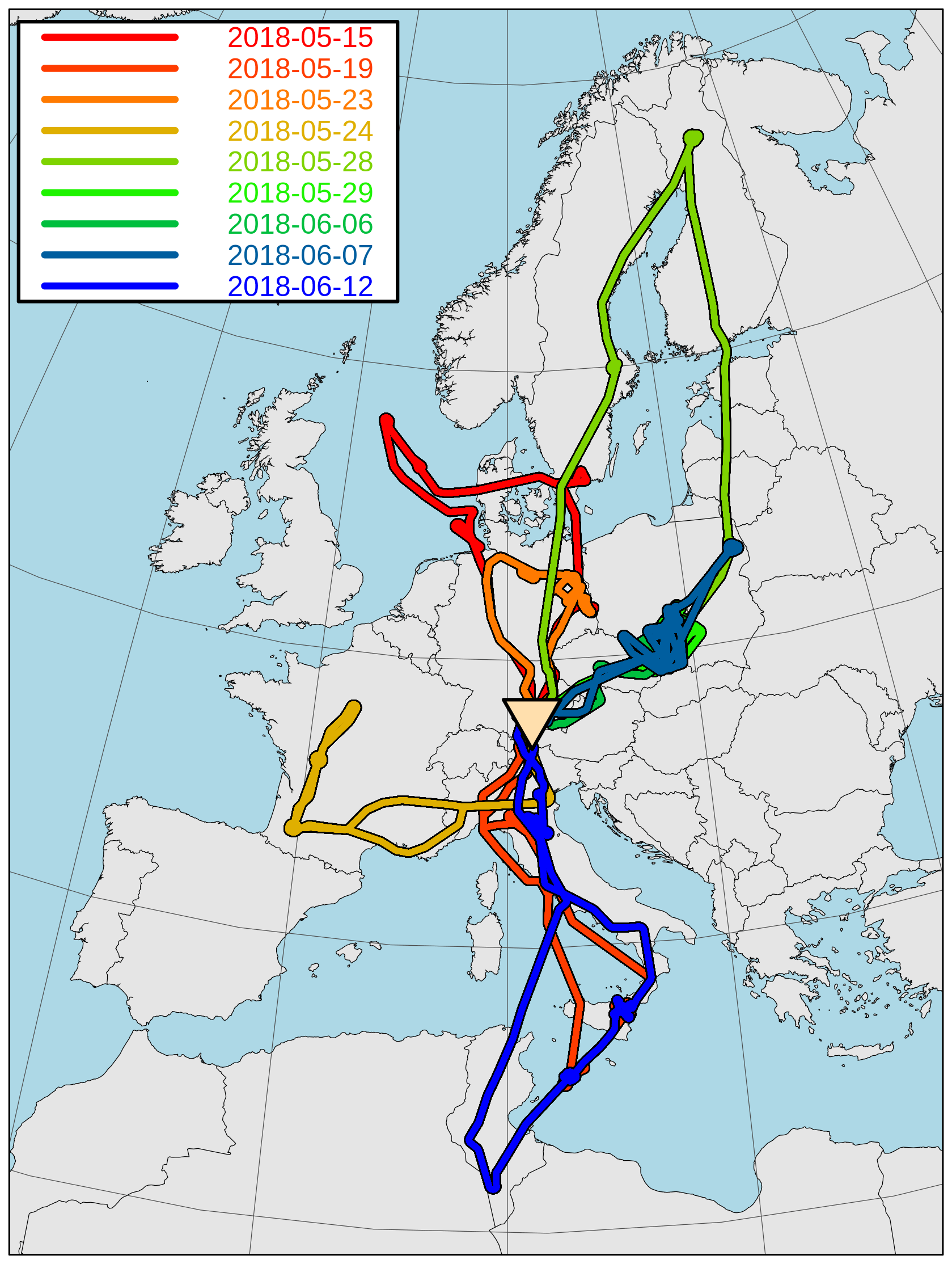
Figure 1Geographical extent of HALO research flights during the CoMet 1.0 mission.
2.2 In situ instrumentation
2.2.1 JIG – Jena Instrument for Greenhouse gas measurements
In situ continuous airborne measurements of greenhouse gases on board HALO have been carried out using JIG (Jena Instrument for Greenhouse gas measurements; photo available in the Supplement, Fig. S1). The core of the device is a modified commercial analyser G2401-m, developed by Picarro Inc. (Santa Clara, CA, USA), which was redesigned in order to fulfil conditions necessary for long-term deployment in the scope of IAGOS ERI (In-service Aircraft for a Global Observing System – European Research Infrastructure). Detailed development of the instrument, with the description of its operational parameters, is described in Chen et al. (2010) and Filges et al. (2015, 2018). Here, only the basic operation principle and main differences to the IAGOS setup are given.
The core method of the measurement is wavelength-scanning cavity ring-down spectroscopy (CRDS), whereby an infrared-wavelength laser light is injected into a high-finesse optical cavity. In the first phase of the measurement, the strength of the incident laser beam gradually increases over time thanks to the resonance effect in the optical cavity, which also allows for the enhancement of the effective absorption length and thus increases the detector's sensitivity. After reaching the designated signal level, the laser is turned off and the ring-down phase of the measurement begins. The time constant of the resulting exponential decay (ring-down time) depends on the absorption coefficient of the measured compound for the laser wavelength, tuned so that the scan along selected individual spectral lines of the measured molecules is possible. The measurement requires the usage of calibration gases, as well as careful control over cavity pressure and temperatures in order to prevent sample density variations. During the measurements described here, the cavity pressure was set at all times to 186.65 hPa (140 Torr) and the temperature to 45.00 ∘C, with tolerance levels of 0.13 hPa (0.1 Torr) and 0.02 ∘C, respectively.
The instrument reports dry mole fractions, defined as the number of molecules of each species in moles per one mole of dry air, with typical observed ranges expressed in micromoles per mole (µmol mol−1) for CO2 (equal to 1 part per million, ppm) and in nanomoles per mole (nmol mol−1) for CO and CH4 (equal to 1 part per billion, ppb). As the collected air was not dried in the sampling line, a water correction was applied based on the online measurements of the H2O mole fraction, following the approach described in previous studies of Filges et al. (2015) and Reum et al. (2019).
Calibration of the instrument was performed in the laboratory before and after the CoMet 1.0 mission by measuring three air mixtures, stored in working tanks, which covered the range of ambient mole fractions of CO2, CH4 and CO and had assignments traceable to the respective WMO calibration scales. All JIG trace gas mole fraction data provided in the current study are reported on the current WMO calibration scales: CO2 X2007, CH4 X2004A and CO X2014A. The instrument calibration was monitored during the mission with the use of two reference in-flight cylinders that contained dry mixtures of atmospheric air of known composition, for each tracer at a high and a low mole fraction, namely 373.4–397.4 µmol mol−1 for CO2, 1661.0–1917.1 nmol mol−1 for CH4 and 77.4–139.5 nmol mol−1 for CO. These were analysed several times during each flight. The calibration cycle consisted of two intervals, each 3 min in length. The first minute of each interval was discarded in subsequent analyses due to pressure equilibration effects within the regulators.
Except for a single calibration check performed prior to take-off during a power-up procedure, all the other calibration check cycles were enabled manually by an onboard operator of the system, during transit phases of the flight, in contrast to the regular IAGOS implementation (Filges et al., 2015, 2018). The in-flight calibration checks occurred at high altitudes, where high gradients of GHGs were not expected and the loss of information could be minimised. The last calibration cycle was always performed immediately before the final approach of the flight. It should be noted that the results of the in-flight calibration checks were only used for assessing a potential drift in the instrument calibration factors relative to the pre-mission (April 2018) and post-mission (November 2018) laboratory calibrations.
Additional, independent verification of the measurement quality was carried out by comparison of the mole fractions from in situ measurements and those obtained from laboratory analyses of air samples collected by the JAS (Jena Air Sampler; see Sect. 2.2.2 and the discussion of the results in Sect. 3.1).
Two malfunctions of the JIG occurred during the CoMet 1.0 mission. On 28 May (flight no. 5), a software issue (i.e. clock reset) caused the loss of 96.8 % of in situ data from that day. The remaining 3.2 % have been excluded from the following analysis due to their fragmentation. The second malfunction occurred during the power-up procedure on 7 June 2018 (flight no. 8), when JIG suffered an unexpected shutdown due to cabin overheating, which required a manual reset of a temperature switch. This in turn caused unintentional damage to the optical fibre mount located inside the instrument housing. The resulting loss of signal strength caused deterioration of the system parameters over flight nos. 8 and 9, increasing noise and shifting the instrument calibration parameters. These were subsequently corrected using in-flight calibrations and post-mission laboratory calibrations. The impact of the malfunction and final effect of applied corrections are discussed in Sect. 3.1.
2.2.2 JAS – Jena Air Sampler
The sampler used during CoMet 1.0 (Fig. S1) is an airborne version of the automated flask sampler developed within the ICOS (Integrated Carbon Observing System) infrastructure. The device is equipped with 12 slots for holding 1 L glass flasks with automatically operated valves at both ends. Sample air, collected outside the aircraft fuselage with a dedicated inlet, flows through tubing (PFA, 415 cm, 6.35 mm ( in.) OD) and into the drying unit (70 cm3, stainless steel) filled with magnesium perchlorate. The dryer is connected via another tubing section (PFA, 317 cm, 6.35 mm ( in.) OD, plus additional 15 cm of 6.35 mm ( in.) OD, stainless steel, for pressure sensor mount) to a Teflon diaphragm pump (N 813.3, KNF Neuberger GmbH) that provides the over-pressure necessary to flush and pressurise the flasks, up to approximately 1500 hPa. The pump is connected directly to the main input manifold (passing through all three rack-mounted sub-units) via another flexible tube (PFA, 156 cm, 6.35 mm ( in.) OD). The input manifold can be connected to the output line either via open flasks (one or more) or a two-way bypass valve. Each flask has its own pair of automated motors responsible for operating its input (upstream) and output (downstream) valves. At the end of the sampler flow line, a mass flow meter (MFM; model D6F-20A6-000, Omron) is installed that integrates the total volume of air flowing through an opened flask, which ensures that the flask volume has been sufficiently flushed with the sampled air (at least 6 L under normal conditions). At the outlet of the system, a pressure release valve is installed that maintains the pressure at 1.5 bar and prevents the backflow of the pressurised cabin air into the sampler in case of power failure. Three pressure sensors and three thermometers are also installed to monitor the status of the system.
The sampler was controlled via computer in the electronic control section using dedicated software. The procedure for flask flushing and filling was enabled manually by an operator, either at predetermined flight altitudes (in the case of measurements of vertical profiles) or locations (e.g. plume sampling). Each flask was flushed with 10 times its volume prior to closing the upstream and downstream valves. Typically, flasks were filled during descending profiles but on some occasions also during ascents. The variable ambient pressure caused the flask fill time to vary between 100 s at high altitudes and 25 s close to the surface.
In order to precisely establish spatio-temporal coordinates from which the sample is collected, a flow model has been used that takes into account (i) flow information from the MFM, (ii) the volume of tubing elements such as the dryer and tubing and (iii) the varying physical length of tubing between the inlet and the flask inlet slots (ranging from 10.76 to 15.58 m). For each collected sample, a temporal weighting function was calculated that represents the collected air volume, following the approach suggested by Chen et al. (2012).
All flasks collected aboard HALO during CoMet 1.0 were analysed in the GasLab of the Max Planck Institute for Biogeochemistry (MPI-BGC) in Jena, Germany, to establish mole fractions of trace gases (CO2, CH4, N2O, H2, SF6) based on their respective WMO scales. Gas chromatographic analysis of air in glass flasks is done with a gas chromatographic system based on two gas chromatographs (GCs; 6890A, Agilent Technologies) equipped with a flame ionisation detector and a nickel CO2 converter (FID) for CH4 and CO2, an electron capture detector (ECD) for N2O and SF6, a helium ionisation pulsed discharge detector (D-3-I-HP, Valco Instruments Co. Inc.) for H2 and a HgO Reduction Gas Analyser (RGA3, Trace Analytical) for H2 and CO. Additional analyses of , and isotopic composition of methane (δ13C−CH4 and δ2H−CH4) were carried out in the IsoLab of MPI-BGC (Sperlich et al., 2016). The typical measurement precision of the laboratory analyses is given in Table 1.
Table 1Average measurement uncertainties of the flasks collected during CoMet 1.0. All values given with coverage probability of 0.68. A correction factor based on Student's t distribution was applied to account for low population size, following the Guide to the Expression of Uncertainty in Measurement (JCGM, 2008).

a Precision calculated as the standard error of the repeated flask measurements (usually between 3 and 5). An average standard error for a complete set of flasks collected during CoMet 1.0 is given. Uncertainty of the scale link specified as the root of the sum of squared uncertainties of (i) specified CCL (Central Calibration Laboratory)-scale transfer uncertainties, (ii) precision limit of individual laboratory standard calibration events, and (iii) response drifts between successive calibration events. For H2, scale transfer uncertainty is equal to zero by definition, as flasks were measured directly against the primary scale. This uncertainty estimate does not include the accuracy of the respective WMO scale.
b and measurements were done on the BGC-IsoLab local realisation of the Scripps scale. Realisation is achieved through the regular measurements of in-house standards against independently calibrated tanks from Scripps. Reproducibility estimate is given as the average of standard deviations calculated from measurements against in-house standards (IsoLab, MPI-BGC, Jena) of three cylinders with air mixtures calibrated independently at Scripps Institute for Oceanography (SIO), covering the range of −262.2 to −807.6 per meg and range of 136.5 to 167.1 per meg.
c Only a single measurement of each sample was possible. Precision estimated using repeated working standard measurements performed in sequence with the sample (usually four or five per sample). Reproducibility defined according to Sperlich et al. (2016).
A significant (approximately 10 nmol mol−1) bias in CO mole fractions was observed when comparing in situ measurements from JIG against gas flasks collected using JAS. Control laboratory experiments run after the campaign have shown that this bias was a result of a growth in CO mole fractions in the period between sample collection and subsequent laboratory analysis. This enhancement in the mole fraction could be attributed to new valve sealing polymer but could not be accurately corrected; therefore we have decided to discard these results. Careful quality control and additional tests did not show any sign of other gases being affected.
2.3 Flight patterns
Depending on the scientific goals set out before each research flight, different flight patterns were executed in order to obtain the most valuable data. The main strategies adopted for the CoMet 1.0 mission were (i) long-range gradient observations, designed to maximise the number of observations for active lidar measurements with CHARM-F operated on HALO; (ii) vertical profiles, aimed mainly at the intercomparison between the lidar and in situ observations; and (iii) low-altitude legs, performed to assess the enhancements of CO2 and CH4 downwind of their sources (plume chasing).
2.3.1 Large-scale variability in upper troposphere and lower stratosphere
Due to the constraints related to using other instruments (the active lidar), a significant amount of flight time was spent flying level at altitudes higher than 4 km, in order to emulate a flight path similar to that of a satellite system. Typical variability of in situ greenhouse gas mole fraction was low in these cases and is usually considered to be caused by the intermixing of air masses coming from different regional source areas. In situ data obtained in this manner are well suited for validation of global chemistry models. As an example, in Sect. 3.2 we compared JIG observations against well established modelling products: CAMS greenhouse gas forecasts. A detailed model description is given in Sect. 2.4.
2.3.2 Vertical profiles
Multiple vertical profiles of the atmosphere were carried out during the campaign in order to establish the connection between column-integrated remote sensing and in situ measurements, thus also linking remote sensing observations to common WMO scales for greenhouse gases. The typical strategy consisted of (i) a high-altitude overflight over a selected target, (ii) descent in the form of a spiral to the lowest possible altitude above the target and (iii) subsequent ascent back to high altitude, usually flown along the shortest path in the direction of the next planned way-point.
Usually two or three vertical profiles were executed during a given flight, depending on the availability of points of interest and airspace accessibility. Wherever possible, profiles were executed above (a) ICOS stations, (b) TCCON stations (Total Carbon Column Observing Network) and (c) Sentinel 5P or GOSAT overpass locations. Flasks were also collected during vertical soundings, at levels distributed between the minimum and maximum altitude, typically consisting of six samples per profile (in some cases reduced to four).
Measurements of vertical profiles are also of high interest for model validation exercises, as the availability of highly precise data on greenhouse gases over Europe is currently still limited. In the scope of the current study, we have assessed the performance of two well-established modelling products (CAMS and Jena CarboScope; see Sect. 2.4) against CoMet 1.0 in situ observations.
2.3.3 Measurements in the planetary boundary layer – plume chasing and isotopic composition
A limited number of data were also collected inside the planetary boundary layer (PBL), usually during the lowest stage of vertical profile sounding. In several cases, however, these PBL sections were extended in order to cross low-level emission plumes (plume chasing). Of particular interest here are the flights over the Upper Silesian Coal Basin (a large regional methane source) and downwind of the Bełchatów coal power plant (the largest single emitter of CO2 in Europe, according to the European Pollutant Release and Transfer Register, v16; E-PRTR, 2019). For both of these sources, clear enhancements from the strong sources were captured when crossing the plume downwind.
Additional to the in situ measurements, flasks were also collected to gather information about additional compounds and the stable isotopic composition of CH4. For the cases in which sufficient data were available, we have applied the method of Miller and Tans (2003), a variation of a classic Keeling model (Keeling, 1958), in order to obtain the isotopic mean source signature (δ0), expressed using relative delta notation. The method assumes a two-factor mixing of background air and methane-enhanced plume:
where δobs is the measured isotopic signature, δbg is the background signature, χobs is the mole fraction of the analysed compound and χbg is the background mole fraction. Here, similar to the Keeling approach, information on δ0 can be gleaned from the application of linear regression; however the source signature is calculated from the slope, rather than intercept, of the linear fit formula. Following the study by Cantrell (2008), we have applied a Williamson–York regression, which allows one to take into account uncorrelated errors in both the x and y axes of the data.
The Miller–Tans method relies on the appropriate assignment of the background signature (i.e. of the atmospheric air outside of the plume). Long-term data available from atmospheric observations show that the isotopic composition of methane in the atmosphere is variable (Röckmann et al., 2016; Nisbet et al., 2019) in both space and time. In order to estimate the background signature, we have used measurements from air samples collected in the immediate vicinity of the target plume, either from the upwind air masses or from outside of the main plume.
2.4 Models
As part of the Copernicus Atmosphere Monitoring Service (CAMS), the European Centre for Medium-Range Weather Forecasts (ECMWF) performs greenhouse gas simulations based on its Integrated Forecasting System (IFS) and provides operational global forecasting products focused on greenhouse gases. In this work, we have used the 5 d high-resolution greenhouse gas forecast product from CAMS (experiment ID: gqpe, downloaded in April 2020; see Agusti-Panareda et al., 2017; Agustí-Panareda et al., 2019) in order to validate the model using our observations. Further in the text, we will refer to these data as CAMS for simplicity. Satellite data were used for initialisation of the forecast, namely TANSO-GOSAT for CO2 and CH4 and additionally MetOp-IASI for CH4 (Massart et al., 2014, 2016). For CO, CAMS operational analysis (Inness et al., 2015, 2019) was used for forecast initialisation. Original CAMS 1 d forecast data, available at the TCo1279 Gaussian cubic octahedral grid (equivalent to approximately 9 km horizontal resolution), were interpolated to . The frequency of the analysed CAMS data was 3-hourly, and vertical resolution was the regular L137 ECMWF configuration.
Additionally, CO2 data were also compared to the Jena CarboScope product (version s04oc_v4.3, Rödenbeck, 2005), further referred to as CarboScope. While the resolution of the driving CarboScope model output fields is much lower in this case ( horizontal), the system benefits from using the fluxes of CO2 optimised using a Bayesian inversion framework. A detailed description of the modelling system is given in Rödenbeck et al. (2003) and Rödenbeck (2005). The transport model TM3, which is used by CarboScope, is described in Heimann and Körner (2003).
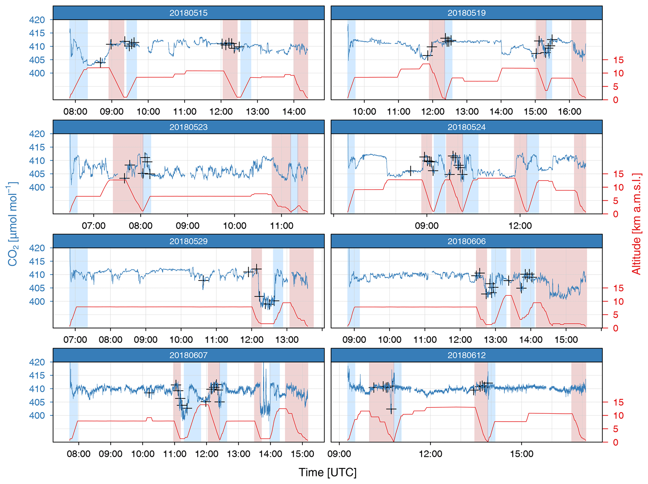
Figure 2In situ mole fractions of CO2 measured throughout CoMet 1.0 with flight altitudes. Shading corresponds to the vertical profiles discussed throughout the paper. Shading colours are denoted as follows: blue – ascending profile, red – descending profile. Co-located flask measurements are marked with black crosses.
3.1 Overview and data quality
A total of 55 h and 17 min of high-frequency (1 Hz) observations of CO2, CH4 and CO were obtained aboard HALO in the scope of the CoMet 1.0 campaign. Measurements of CO2 are presented in Fig. 2, and a full overview, including also CH4 and CO, is available in the Supplement (Fig. S2). Observations were performed at altitudes ranging from approximately 50 m up to 14 km above mean sea level. Data from 51 vertical profiles are available, of which 21 have simultaneous flask measurements. They are listed in the Supplement (Table S1). A total of 15 in-flight calibrations were performed, making it possible for the single-measurement precision to be estimated for flights no. 1–7. These were equal to 0.06 µmol mol−1 (CO2), 0.3 nmol mol−1 (CH4) and 3.1 nmol mol−1 (CO). Malfunction during the roll-out procedure prior to flight no. 8 caused deterioration in the instrument noise for two subsequent flights (nos. 8 and 9), with values of precision increasing to 0.3 µmol mol−1, 1.5 nmol mol−1 and 50 nmol mol−1 for CO2, CH4 and CO, respectively.
Results from in-flight measurements of the two reference cylinders showed no significant drift; however the flight-to-flight variation of each low- and high-span measurement during the period prior to the instrument malfunction on 7 June was slightly larger than expected for CO2: low-span measurements varied by 0.10 µmol mol−1, 0.4 nmol mol−1 and 1.0 nmol mol−1, while high-span measurements varied by 0.14 µmol mol−1, 0.3 nmol mol−1 and 0.8 nmol mol−1 for CO2, CH4 and CO, respectively. The likely cause for this is the silicon rubber membranes used in the pressure regulators (Filges et al., 2015), which are known to cause diffusion of CO2 (Hughes and Jiang, 1995). Given that species other than CO2 did not show unexpected behaviour, we did not apply any correction of the measurements resulting from the in-flight measurements of the reference cylinders. For this reason, we also did not apply any correction of drift within each flight, in contrast to the experience of Karion et al. (2013b).
The comparison between flask and in situ measurements is available for all except one flight (no. 5). From the 96 samples collected and analysed, 84 had simultaneous in situ measurements available from JIG that could be used for a bias assessment. Here, we compare bias between both our data sets to the “network compatibility goal”, defined by the World Meteorological Organization as “the scientifically determined maximum bias among monitoring programmes that can be included without significantly influencing fluxes inferred from observations with models” (WMO, 2019). WMO specifies this compatibility goal as being equal to 0.1 µmol mol−1 for CO2 (in the Northern Hemisphere) and 2 nmol mol−1 for both CH4 and CO.
As shown in Fig. 3, the average bias for flights 1–7 was equal to −0.131 (30) µmol mol−1 for CO2 and −2.93 (32) nmol mol−1 for CH4, where numbers in parentheses represent standard uncertainty in the final digits quoted for the numerical value. Larger spread when independent measurements are considered (Fig. 2) stems mainly from the imperfect match between the temporal coordinates of the two instruments, which can be considered random and does not cause systematical shift. After the malfunction (see Sect. 2.2.1), i.e. for flights no. 8 and 9, these mean offsets were equal to 0.127 (68) µmol mol−1 and −0.64 (91) nmol mol−1 for the respective gases. While the difference of values as compared to flights 1–7 is statistically significant, it is still close to the WMO compatibility goal.
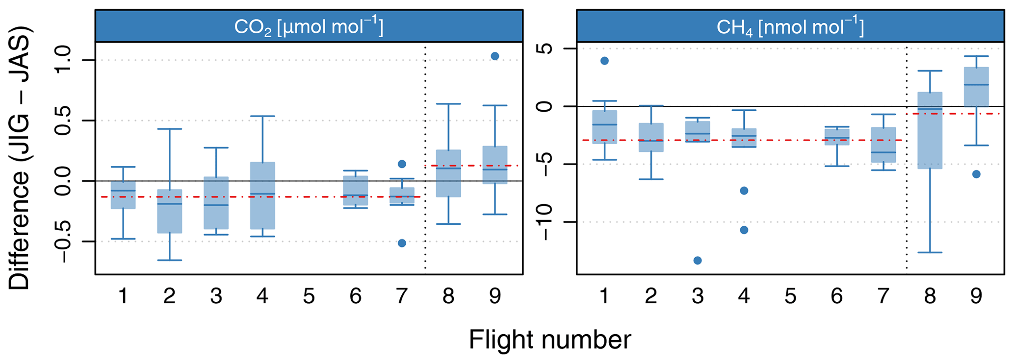
Figure 3Comparison between JIG results and analysis of flasks collected during CoMet 1.0 aboard HALO. Data from the last two flights (separated by the dashed line) indicate a residual change in calibration, following an instrument malfunction. See text for details.
3.2 Large-scale variability
Out of the total number of observations during CoMet 1.0, 84 % were performed at altitudes above 4 km and are of particular interest for model validation. To demonstrate the utility of the observations to validate model results, as well as to help understand the patterns in measured mole fractions, we analyse and compare JIG measurements to CAMS high-resolution products for CO2, CH4 and CO. Flight no. 2 (shown in light red in Fig. 1) is discussed as an example.
The flight (Fig. 4a) was executed on 19 May 2018, with the main goal of capturing the large-scale variability of greenhouse gases in the atmosphere above Italy and the Mediterranean coast. Two vertical profiles were planned above ICOS stations, namely Lampedusa (35∘31′05′′ N, 12∘37′50′′ E) and the Monte Cimone mountain station (Tuscan–Emilian Apennines; 44∘11′380′′ N, 10∘42′050′′ E). The latter profile was executed approximately 20 km away from the target due to an active thunderstorm over the site. Other points of interest were the Po Valley, crossed twice (morning and afternoon) at high altitude, and two high-altitude circles around Mount Etna (35∘31′050′′ N, 12∘37′500′′ E).
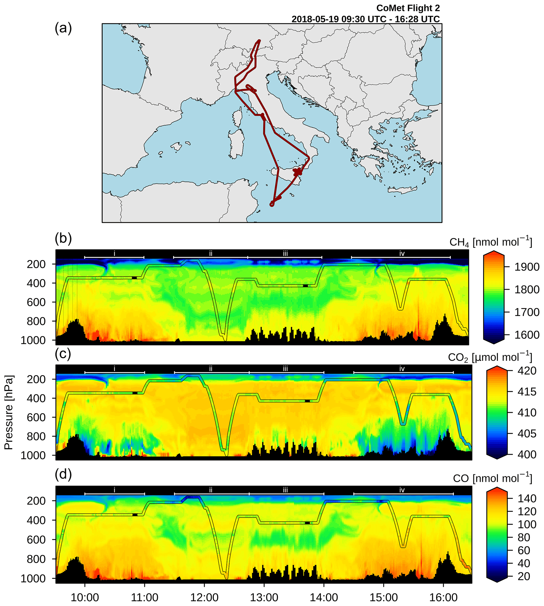
Figure 4Curtain plot showing results for 19 May 2018. (a) Overview map with flight path. Time series of aircraft altitude, with CAMS model results as colour plot in background for (b) CH4, (c) CO2 and (d) CO; coloured lines superimposed on the curtain plot denote in situ measurements from HALO, with mole fractions plotted in the same colour scale. Ranges labelled (i) to (iv) within the panels denote distinct sections of the flight as follows: (i) initial southward crossing of the Po Valley, (ii) passage over Mediterranean towards Lampedusa ending with a vertical sounding near the ICOS station, (iii) circular flights over Mt. Etna, (iv) northward flight over northern Italy with a profile attempted over Mt. Cimone. See the discussion in the text for details.
Figure 4b–d show the CAMS model results extracted at the geographical aircraft time and location, together with corresponding in situ observations from JIG overlaid on the aircraft flight path, both plotted using the same colour scale. The model captures most of the features observed in the atmosphere. Speaking in terms of observed spatial and temporal variability of the atmospheric composition (modelled and observed), four sections of the flight can be identified: (i) morning overflight over northern Italy; (ii) passage over Mediterranean Sea, ending with a vertical sounding at Lampedusa; (iii) circling Mount Etna at medium altitude; and (iv) northward flight over Italy, including a vertical profile in the vicinity of Monte Cimone, with a subsequent crossing of Po Valley and the Alps, ending with landing at home base.
During the first section of the flight (Fig. 4, i), after the initial climb, the aircraft stayed at high altitude (300 hPa, approximately 8 km a.m.s.l.), sounding the free troposphere above the Po Valley. Comparison of measured concentrations to the model suggests that the chosen flight level was well within the free troposphere. Close to the surface, CAMS predicted high enhancements of greenhouse gases, clearly visible on the CH4 and CO plots. At the time (10:00–11:00 UTC), the boundary layer was still developing, reaching only about the 900 hPa level (approximately 1000 m).
After crossing the coastline, the aircraft ascended to a cruise altitude of 250 hPa (approximately 12 km). Around 11:30 UTC it reached the tropopause level and, after another increase in altitude, entered into the stratosphere for approximately 10 min immediately prior to the vertical sounding at Lampedusa (Fig. 4, ii). The vertical structure of the atmosphere was generally well predicted in the model (see Sect. 3.4 and also Figs. S3–S18), albeit larger differences can be observed in the lowest 3 km of the profile, especially for CO2.
The Mt. Etna section of the flight (Fig. 4, iii) took place mostly in the free troposphere, and no significant gradients were observed for either of the measured compounds. Subsequent transfer over southern Italy (iv) started with an ascent into the stratosphere (at approximately 220 hPa, 13 km a.m.s.l.). After 10 min of northward flight, the aircraft crossed into the troposphere horizontally again.
Immediately before the descent to Monte Cimone, it crossed a stratospheric air filament, possibly brought down to the flight level by the outflow of a deep convective system active in the area in the afternoon on that day. This is corroborated by CAMS model results, which show a clearly defined air-mass structure, depleted in mole fractions for all the observed compounds, stretching from the stratosphere at 200 hPa down to approximately 400 hPa (corresponding to roughly 13 and 8 km a.m.s.l., respectively). Shortly after that, the aircraft descended, making a downward spiral over the northern Apennines, down to approximately 700 hPa (3.5 km). The model–observation discrepancy is much higher at this point, most probably due to (i) errors in representation of the local convective systems or (ii) errors in the surface fluxes driving the modelled mole fractions or a mixture of both. The high-resolution CAMS product correctly captures most of the large-scale phenomena. There are, however, specific situations in which the performance of the model drops, specifically in the vicinity of strong local convection systems, where parameterisations can sufficiently predict neither the height nor the transport of the strong enhancements present in the Po Valley. The reasons behind this discrepancy may stem from the inability of coarser scale parameterisations to capture local phenomena accurately or from an incorrect distribution of the ground-level sources.
In the following section, we analyse the model–data mismatch more closely using the subset of CoMet 1.0 data collected only during the vertical soundings.
3.3 Vertical structure of the atmosphere
All profiles of CO2, CH4 and CO collected with JIG are presented in Fig. 5, together with comparison to the CarboScope and CAMS model products. Individual comparisons are available in the Supplement (Figs. S3–S10 and S11–S18). It should be noted that the mean profile for the lowest altitudes is dominated by a limited number of cases when the ground level was reached. This happened most often at home base (EDMO, Oberpfaffenhofen). Similarly, only a limited number of profiles reached altitudes beyond 12 km a.m.s.l.
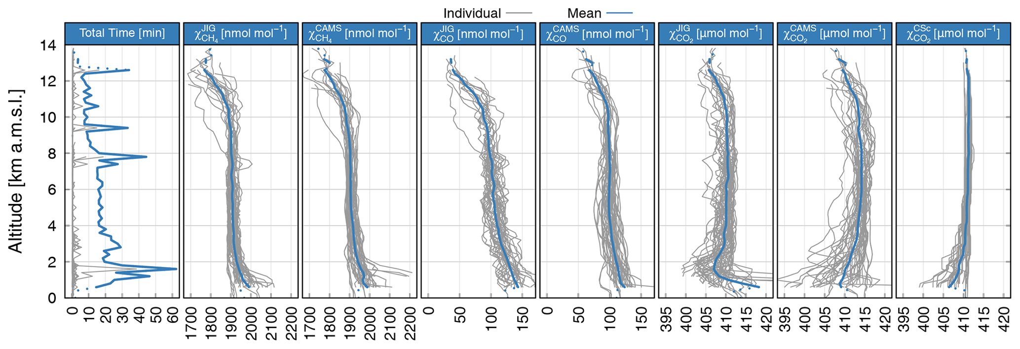
Figure 5An overview of the vertical profiles measured during the CoMet 1.0 mission, together with modelled profiles from CAMS and CarboScope (denoted with CSc). In the first panel, total time is calculated as a sum of 1 s observations from each respective bin. All the other panels present mole fractions for different variables, binned into 200 m layers. Averages for each layer are shown as a solid blue line, while solid grey lines represent individual profiles. Dashed lines represent the means with less than 200 s of observations available. Only data from the individual profiles marked on Fig. 2 are plotted here; i.e. the measurements collected during horizontal sections of the flights are not included.
Again, three distinct altitude ranges can be distinguished based on the observed gas mole fractions and their variance. The lowest, the PBL, is characterised by highly variable concentrations and is located in the altitude range of 0–3 km. Both the highest and lowest observed concentrations of CO2 were observed here, with most of the observations in the range between 400 and 420 µmol mol−1. Occasionally, peaks of over 420 µmol mol−1 were observed in the vicinity of strong point sources (e.g. Bełchatów power plant). CH4 and CO variability were also high, with most observed values between approximately 1880 and 2000 nmol mol−1 for methane (with peaks above 2100 nmol mol−1) and 100–150 nmol mol−1 for carbon monoxide.
Above the PBL range, free tropospheric observations were characterised by much smaller variability. For CO2, the mean profile becomes flat, with a value of 410 µmol mol−1 up to approximately 10 km altitude. For CH4 and CO, a vertical gradient in the mean values is observed, reflecting the balance between surface anthropogenic sources, large-scale advection and tropospheric chemical sinks.
Above the altitude of 10 km, a more pronounced decrease in the mole fractions is observed, which is directly related to occasional crossings into the tropopause region and the lowermost stratosphere. The variability of the observed decrease is large and follows the variability in the tropopause height. On average we have observed a 4 µmol mol−1 decrease for CO2 between 10 and 13 km, which is most probably caused by the increasing age of the slow-mixing stratospheric air (Andrews et al., 2001). Decreases of CH4 and CO are more pronounced (on average 150 and 70 nmol mol−1, i.e. 8 % and 45 % relative to the value at 10 km), underlining an increased oxidative breakdown of these tracers (added to the age effect in case of CH4).
While the observed gradient is similar to previously reported studies (e.g. Wofsy, 2011; Sweeney et al., 2015; Umezawa et al., 2018), measurements from CoMet 1.0 also clearly indicate the increase in atmospheric concentrations over the past years. For example, the CH4 mole fractions measured during the IMECC campaign in autumn 2009 (Geibel et al., 2012) were approximately 60 nmol mol−1 lower throughout the atmospheric column than those observed in 2018. This number is closely in line with the mean global atmospheric growth of methane of 63.8 nmol mol−1 (between 2009 and 2018; NOAA, 2020).
3.4 Model validation
The vertical profile subset of the measurements was the basis of the comparison to the well-established global modelling systems CAMS and CarboScope. Here, we focus on describing the vertical structure of the model–data mismatch, defined as the difference between the modelled results and in situ observations from JIG, presented in Fig. 6. Mirroring previous discussion of different characteristics of the atmosphere, here the different nature of discrepancies can also be separated into three distinct layers of the atmosphere. It is worth noting that the model–observation mismatch is, in general, constant in neither space nor time, as can be seen when analysing the variability between different flight days. However, some important conclusions can be drawn when analysing the overall vertical structure in the difference between global model results and CoMet 1.0 in situ observations.
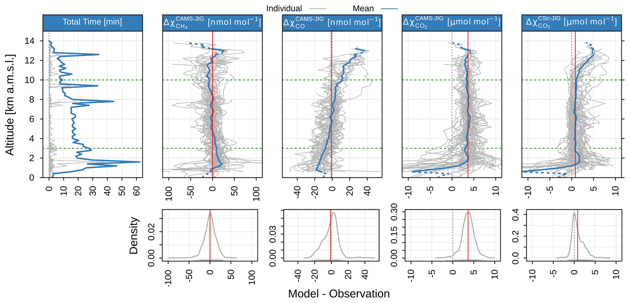
Figure 6Top row: the first panel shows time spent in each altitude bin (200 m) for individual flights (grey lines) and the sum for CoMet 1.0 (solid blue). The four panels to the right show differences between modelled (CAMS and CarboScope, latter abbreviated as CSc) and measured mole fractions as a function of altitude (grey – individual flights, blue – average per altitude bin). Dashed red line represents the average value in the altitude range 3–10 km (vertical range marked with horizontal dashed green lines). Bottom: density plots for measurements in the free tropospheric (3–10 km) range.
The variability in the mismatch is highest closest to the surface (bottom 3 km), which is related to influences from local sources and sinks as well as variability of atmospheric mixing and transport in the PBL, which are hard to represent at respective model resolutions ( for CAMS, for CarboScope). Another source of mismatch is related to uncertainties in the emissions data used by the models. Validation of individual emission sources, while of critical importance, remains challenging. In addition, in the case of biospheric CO2, the prediction of fluxes on scales relevant for direct comparison of mole fractions on regional scales also remains a difficult task. This is true for all the analysed compounds and both models, with a markedly larger discrepancy in the CarboScope product that clearly suffers as a result of its low spatial resolution. As the in situ measurements from CoMet 1.0 are not numerous enough to give a robust estimate for the European region, and differences between the model predictions and observations will be heavily dependent on a specific synoptic range and distribution of sources in the vicinity, we do not provide any general statistics for this lowest part of the atmosphere.
In the free tropospheric range, the mismatch represents the large-scale offset between the model and observations better and is only weakly dependent on the spatial distribution of the emissions sources. Under this assumption, the mismatch is mostly caused either by (i) large-scale (i.e. at least national) offsets in emission strengths; (ii) bias in the initialisation of the forecasted fields (with CAMS GHG and operational analysis fields which are a combination of model simulation and satellite observations); or (iii) errors in chemistry parameterisations (OH radical reaction chains, CH4 and CO).
In the CAMS product, the offset between the modelled values and observations in the troposphere becomes stable with height for CH4 and CO2, with a symmetric distribution around a mean value (CH4: 0 (14) nmol mol−1; CO2: 3.7 (1.5) µmol mol−1, where standard uncertainty in the final digits is given in brackets. For CO2, a substantial offset is still present, most probably connected with errors in the strength of the net biospheric fluxes predicted in the model. This general offset needs to be taken into account if the data are either compared directly to the measurements (this paper) or used as lateral boundary conditions for regional modelling studies. For CO, a sloped model–data mismatch is observed, most likely related to known issues with the inventories of anthropogenic emissions of CO (e.g. Boschetti et al., 2015) superimposed on chemistry-related effects. The mean value of the offset of CO in the 3–10 km altitude range is equal to −1.0 (8.8) nmol mol−1.
For altitudes above 10 km, the mismatch between CAMS and observations shows larger variability for CH4 and CO, with CO2 discrepancies similar to those observed in the free troposphere. While the number of observations at these higher altitudes is relatively low compared to those below 10 km, we believe that these differences are also caused by errors in both transport and chemistry schemes in the IFS system. These have been investigated in some detail in the case of CH4, for which the errors in the stratosphere have been found to be larger than those observed in the troposphere (Verma et al., 2017).
Optimised CO2 mole fractions from CarboScope also show overall good agreement when compared to observations, despite lower model resolution compared to CAMS. The model–data mismatch is dominated by a random term in the free tropospheric range (0.8 (1.3) µmol mol−1). Interestingly, the distribution of the mismatch in this altitude range is a positively skewed Gaussian curve (Fig. 6, bottom-right panel), with the values in the main peak almost symmetric around 0 µmol mol−1 and the mean offset in the 3–10 km range driven by the values in the tail of the distribution. The most probable cause is the inability of the model to represent convective uplifting of CO2-depleted air from the PBL. It should also be noted that in the CarboScope product, a systematic over-prediction of CO2 mole fractions above 10 km (up to 5 µmol mol−1) is observed, which might be caused either by (i) significant errors in the tropopause height or (ii) vertical mixing in the lower stratosphere that is too fast, leading to underestimation of the gradient and the chemical age of CO2. In the PBL range, the mole fractions are generally underestimated, sometimes by more than 10 µmol mol−1, albeit such a large discrepancy is only visible for the lowest altitude range (less than 1 km), where the sample size is low. Where the observation set is more robust, the bulk of observations is characterised by differences smaller than 10 µmol mol−1 and can have either positive or negative sign. Such behaviour is to be expected when trying to compare local plume enhancements to the low-resolution model results that averages over large, inhomogeneous areas characterised by a dynamic spatio-temporal diurnal cycle of fluxes.
3.5 Additional data from discrete samples – JAS
Figure 7 presents additional data acquired throughout the campaign with discrete samples, with a detailed overview provided in the Supplement (Fig. S19 and Table S1). Apart from CH4 and CO2, for which the flask data were used for validation, important constituents were monitored, offering further insights into the state of the atmosphere over Europe during the CoMet 1.0 mission. The general nature of the collected data follows the patterns described for in situ data, with three distinct abundance regimes: (i) PBL, (ii) residual layer/free troposphere and (iii) tropopause and lower stratosphere, however with some marked differences.
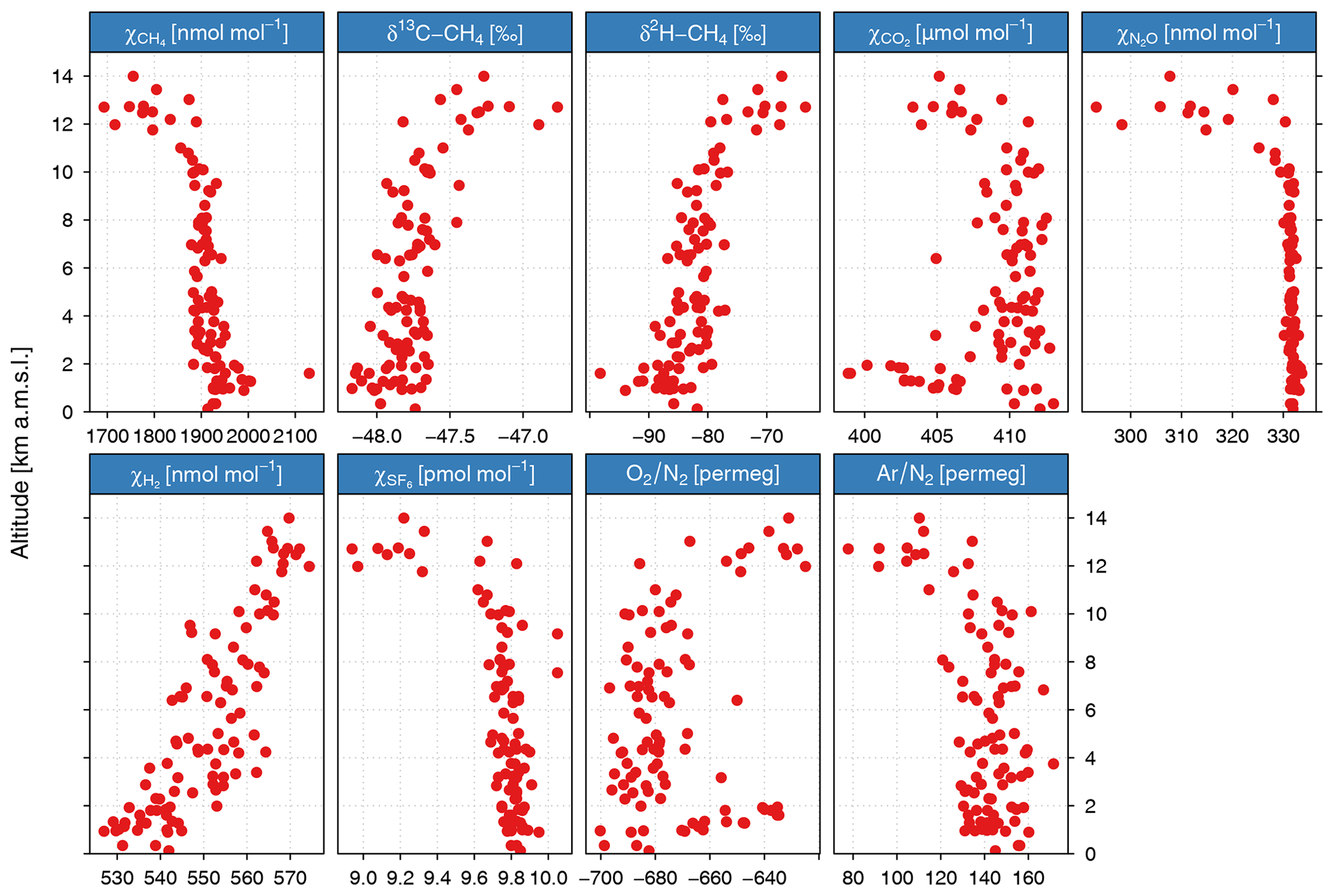
Figure 7Combined results of air composition as measured in flask samples collected during CoMet 1.0 aboard HALO.
For N2O and SF6, both potent greenhouse gases (IPCC et al., 2013), there is no clearly visible mole fraction gradient between the PBL and the free troposphere. For both gases, the variability is known to be dominated by the slow stratospheric transport, effectively causing the “age” of air masses to be higher than the tropospheric air below (Andrews et al., 2001). For N2O, this effect is superimposed on the additional signal caused by its photochemical destruction in the stratosphere. Notably, during CoMet 1.0, two samples were collected with SF6 mole fractions elevated by approximately 0.2 pmol mol−1. The first was filled on 7 June, at 9.2 km altitude, over Czechia, and second on 12 June, at 7.6 km, during the downward profile over the Po Valley. The potential source of these two observations might be worth investigating, especially in light of the constant atmospheric increase of the SF6, despite substantial efforts to curb emissions of this potent greenhouse gas (Weiss and Prinn, 2011). Some attention was also given to molecular hydrogen (H2) due to its potential feedbacks to the atmosphere oxidative capacity and stratospheric ozone levels (see Batenburg et al., 2012, and references therein). Values measured during the mission, namely 540 nmol mol−1 near the surface, approximately 550–560 nmol mol−1 throughout the free troposphere and approximately 570 nmol mol−1 in the lower stratosphere, are comparable to previously reported values, e.g. in the scope of the CARIBIC project (Batenburg et al., 2012). This structure is driven by the presence of a relatively strong soil sink in the latitude band covered during CoMet 1.0, as has been confirmed by modelling studies (e.g. Pieterse et al., 2011). and ratios are presented for completeness but are not discussed in the present study.
Of particular interest during CoMet 1.0 was the stable isotopic composition of methane. Abundances of both δ13C−CH4 and δ2H−CH4 are strongly and negatively correlated ( and , respectively) with mole fractions of methane, signifying the potential to use the isotopes as a marker of the source processes. Indeed, in the next section we present an application of using isotopic composition to differentiate between specific source types in the study area of the Upper Silesian Coal Basin (USCB, southern Poland).
3.6 Capturing the USCB source signature with isotopic data
Due to the broader spatial range covered by the HALO aircraft, the number of samples taken over the USCB area using the JAS instrument was limited to 12 flasks, collected over two flights performed on 29 May and 6 June 2018 (HALO flights 6 & 7, respectively). The main effort of flask sampling over USCB was carried out using another platform, namely FDLR Cessna (see Fiehn et al., 2020), aboard which a twin instrument was installed that allowed for a batch of approximately 60 samples to be collected, most of them inside the PBL. In the following paragraphs we only discuss samples collected on HALO. A broader discussion of methane isotopic composition observed during CoMet 1.0 will be a part of an upcoming study.
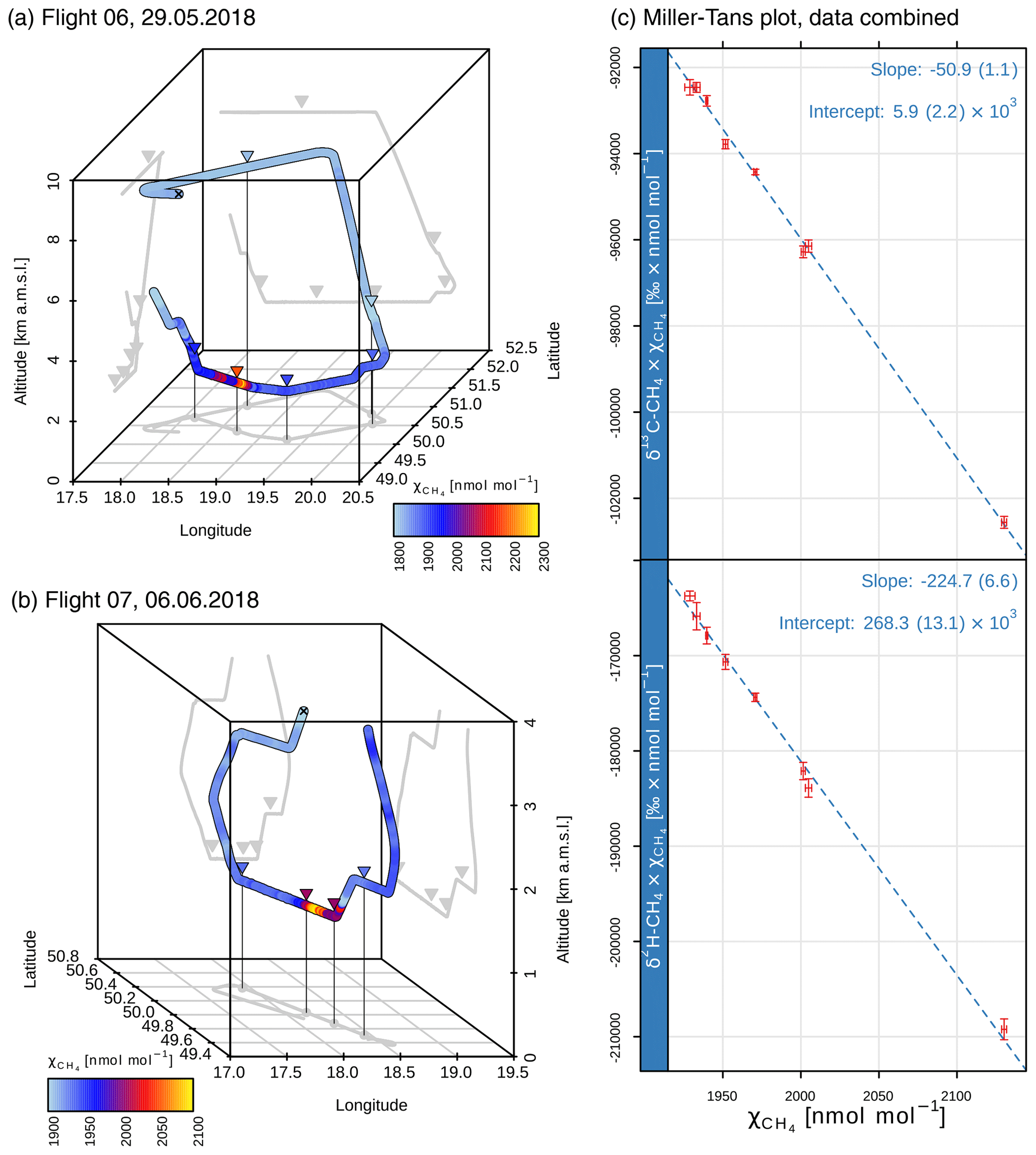
Figure 8(a, b) Visualisation of CH4 measurements over USCB during flights no. 6 (a) and no. 7 (b). For flight no. 7, only data from below 4 km altitude are plotted for clarity. Coloured lines represent mole fractions along the flight path, with the first plotted measurement marked with “x”, and triangles show the flask sampling locations. Both in situ and flask mole fractions are coloured using the same scale. (c) Miller–Tans model of isotopic source signatures for δ2H and δ13C, based on eight flask samples collected below 3 km over the USCB during flight nos. 6 and 7 together. See text description for details. The dashed line is the linear fit using the Williamson–York formula (Cantrell, 2008). Values of fit parameters are given with 1σ uncertainty in the parentheses.
During flight 6 (Fig. 8a), the aircraft crossed the USCB at approximately 8 km altitude then turned south-eastwards during the descent down to ca. 2 km, where it crossed into the PBL. Then, after turning south-westward, it crossed the USCB area upwind of the coal-mine sources at 1800 m, and, after another turn to north-west, it crossed the study area again, this time downwind of the known source locations. Along the flight path, six flasks were collected: two in the free troposphere during the high-altitude overpass and the descent, respectively, then two during the upwind crossing in the PBL and another two during the final downwind crossing inside the PBL. During flight 7 (Fig. 8b), a similar pattern was executed, with the exception that no upwind crossing in the PBL section was executed. Again, two flasks were collected in the free troposphere immediately before and during the descent (at altitudes of 7.6 km and 4.3 km a.m.s.l., not shown on the plot), and four subsequent samples were collected during the PBL section, flown at an altitude of 1400 m for the most part, until the aircraft was forced to ascend to approximately 2 km after crossing into the airspace of Czechia.
A comparison between patterns of in situ mole fractions and flask collection locations clearly shows that air masses with CH4 mole fractions significantly enhanced by local sources were sampled at least three times. We have aggregated measurements from both days, assuming that the enhancement is coming from the same source (or source cluster), which is partially corroborated by wind observations (not shown) and modelling analyses supporting the campaign (Nickl et al., 2020; Gałkowski et al., 2021). Application of the Miller–Tans approach (Fig. 8a) yields an isotopic signature for the USCB source of (6.6) ‰ and (1.1) ‰. Again, standard uncertainty in the final digits is given in brackets.
These values can be compared to previously published data. A comprehensive data set, gathering published values of isotopic signatures from various methane sources, has been compiled and described by Sherwood et al. (2017). Most of the information it contains came from studies focused on methane emitted from fossil fuel extraction (including regular oil drilling, shale gas extraction and gas emitted during coal mining), but data on biomass burning and biogenic sources are also included. Figure 9 shows the main ranges of these source signatures together with flask data collected during CoMet 1.0. Fossil-related methane sources are marked with rectangles (representing main ranges of the reported data and not their full extent) and biogenic source signatures as points (with bars marking the standard deviation of the reported signatures). As can be seen, the values reported in this study (marked with blue point with 1σ ellipse) fall into the typical range reported in Sherwood et al. (2017), in the middle of conventional anthropogenic methane sources characterised by relatively high δ2H (in contrast to the second cluster with δ2H values closer to −300 ‰).
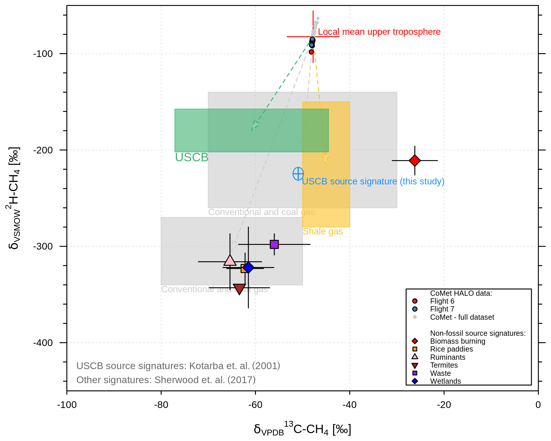
Figure 9Isotopic composition of methane measured over the USCB (red and blue points) compared to source signatures estimated in this study using the Miller–Tans method (light blue cross with 1σ uncertainty ellipsis) and previously reported ranges of isotopic composition for the dominant methane source groups. For the Miller–Tans method, the background signature was estimated using available measurements from the free troposphere (red cross). Data on global source signatures are based on Sherwood et al. (2017). Coloured blocks denote the approximate broad ranges of values reported there for coal and conventional gas excavation (purple), shale gas excavation (orange) and biomass burning (blue). Selected biogenic source signatures are also marked as points, with whiskers denoting the standard deviation of values reported in Sherwood et al. (2017). Data reported previously for USCB coal-mine sources by Kotarba (2001) are marked with a green rectangle.
We also compared our results against signatures from the same area published previously. Measurements of methane, with samples collected in the coal-mine tunnels, were performed by Kotarba (2001). Their study encompassed measurements of methane isotopic composition from a total of 15 mines in the USCB (with δ2H measured in all but one), including samples collected from different coal seams. For the purpose of this study we have aggregated distinct samples reported in the original study and calculated mine-specific averages, which yielded a total range of δ2H between −202.0 ‰ and −157.5 ‰. Reported values for δ13C were between −77.1 ‰ and −44.5 ‰. These have been marked in Fig. 9 with a green rectangle labelled “USCB”.
In recent years there has also been a significant effort to constrain the USCB coal-mine source signatures, as many of the mines reported upon in Kotarba (2001) have been closed over the years, and those that remained open have completed the excavation of the old deposits and moved to different ones, possibly with different isotopic signatures. The results of these more recent measurements, representing methane emitted from 23 different coal-mine shafts, have yielded mean values of the signatures ( (5.7) ‰, (46.3) ‰, brackets showing standard deviation), indicating that the methane emitted there has shifted to lower deuterium signatures (with almost unchanged values of δ13C), corroborating the value reported in the present study. A more detailed discussion on these recent measurements will be presented in an upcoming study by Stanisavljevic et al. (2021, this special issue).
A high-resolution in situ system for online observations of greenhouse gases (JIG) was successfully deployed during the CoMet 1.0 mission aboard the German research aircraft HALO aircraft over continental Europe. More than 55 h of high frequency (1 Hz) observations of CO2 and CH4 and over 38 h of CO observations were collected over the course of nine flights between 15 May and 12 June 2018. In addition to in situ observations, 96 discrete flask samples were collected and analysed for atmospheric composition, including δ13C and δ2H isotopic signatures of methane. Careful pre-flight, in-flight and post-flight calibration procedures allowed us to obtain a highly precise (single-measurement standard deviations: 0.06 µmol mol−1 for CO2, 0.3 nmol mol−1 for CH4 and 3.1 nmol mol−1 for CO) data record that is traceable to international WMO calibration scales. Comparison with flask samples analysed in the laboratory confirms that the measurement data are close to compliance with the WMO compatibility goals (average bias smaller than 0.15 µmol mol−1 and 3 nmol mol−1 for CO2 and CH4, respectively).
Observations collected during the mission were used in combination with two of the available modelling products (CAMS and CarboScope) to explain the observed atmospheric variability on both regional scales as well as during the localised vertical soundings (a total of 50 throughout the campaign), covering altitudes from ground level to 14 km a.m.s.l.
Independent validation of available model products showed overall good agreement between observations and global state-of-the-art products, with very good agreement for CH4 and CO2 in the free troposphere/residual layer range (3–10 km) and slightly (CAMS) to significantly (CarboScope) worse performance in the PBL and the stratosphere. These results highlight (i) the inability of the coarse-grid models to represent local sources and processes influencing individual profiles (in particular for CarboScope but also clearly visible in the relatively high-resolution CAMS product) and (ii) challenges in the high-resolution modelling of biospheric fluxes of CO2.
We have also demonstrated the potential of using isotopic signatures measured in the downwind plume for source attribution. Samples collected during two flights above one of the main target areas of the CoMet 1.0 mission, the USCB, have clearly pointed to coal mining as the main source of the observed methane enhancement ( (1.1) ‰, (6.6) ‰). It should be noted that while the measured deuterium signatures are substantially lighter than has been reported in previous studies from the area, they correspond to more direct estimates performed in the scope of CoMet 1.0 by other teams involved (Mila Stanisavljevic, personal communication, 2020), highlighting a shift in isotopic emission signatures following changes in coal-mining activities, e.g. the closure of coal mines or changes of excavated coal beds/seams.
The code used for data processing and analysis is available from the first author upon request. The data collected during the mission are available from the HALO database at https://doi.org/10.17616/R39Q0T (last access: 5 January 2021; re3data.org, 2021). They are part of the Carbon Dioxide and Methane Mission for HALO (CoMet) dataset, used in its latest version available at the moment of submission of the manuscript. Currently, access to this data is available by request. After project completion they will become freely accessible.
The supplement related to this article is available online at: https://doi.org/10.5194/amt-14-1525-2021-supplement.
MG collected the data and prepared the manuscript, with contributions from all co-authors. MR and AJ assisted with flask sample collection and performed the analyses. AA-P supplied CAMS model data and assisted with data interpretation. JM, FTK and JC contributed to the mission planning and data analysis. CG co-designed the CoMet 1.0 mission, collected the data and provided critical input to the manuscript. AF coordinated all CoMet campaign activities.
The authors declare that they have no conflict of interest.
This article is part of the special issue “CoMet: a mission to improve our understanding and to better quantify the carbon dioxide and methane cycles”. It is not associated with a conference.
We would like to express our appreciation to all the people involved in the CoMet campaign, without whom the campaign could not succeed. In particular we would like to thank DLR-FX for the campaign management, the pilots of the HALO aircraft, our colleagues at AGH University of Science and Technology and all the staff at MPI-BGC involved in the flask measurements. We also want to thank Mila Stanisavljevic for providing information on the isotopic composition in USCB and acknowledge the use of resources of Deutsches Klimarechnungszentrum (DKRZ), namely the high-performance cluster Mistral, for data storage and analysis.
This research has been supported by the Max Planck Society (MPG), the German Aerospace Center (DLR) and the German Federal Ministry of Education and Research (BMBF) through project AIRSPACE (grant nos. FKZ 390 01LK1701A and FKZ 390 01LK1701C), as well as the German Research Foundation (Deutsche Forschungsgemeinschaft, DFG Priority Programme SPP 1294 “Atmospheric and Earth System Research with the High Altitude and Long Range Research Aircraft HALO”).
The article processing charges for this open-access
publication were covered by the Max Planck Society.
This paper was edited by Abhishek Chatterjee and reviewed by two anonymous referees.
Agusti-Panareda, A., Diamantakis, M., Bayona, V., Klappenbach, F., and Butz, A.: Improving the inter-hemispheric gradient of total column atmospheric CO2 and CH4 in simulations with the ECMWF semi-Lagrangian atmospheric global model, Geosci. Model Dev., 10, 1–18, https://doi.org/10.5194/gmd-10-1-2017, 2017. a
Agustí-Panareda, A., Diamantakis, M., Massart, S., Chevallier, F., Muñoz-Sabater, J., Barré, J., Curcoll, R., Engelen, R., Langerock, B., Law, R. M., Loh, Z., Morguí, J. A., Parrington, M., Peuch, V.-H., Ramonet, M., Roehl, C., Vermeulen, A. T., Warneke, T., and Wunch, D.: Modelling CO2 weather – why horizontal resolution matters, Atmos. Chem. Phys., 19, 7347–7376, https://doi.org/10.5194/acp-19-7347-2019, 2019. a
Ahmadov, R., Gerbig, C., Kretschmer, R., Koerner, S., Neininger, B., Dolman, A. J., and Sarrat, C.: Mesoscale covariance of transport and CO2 fluxes: Evidence from observations and simulations using the WRF-VPRM coupled atmosphere-biosphere model, J. Geophys. Res., 112, D22107, https://doi.org/10.1029/2007JD008552, 2007. a
Amediek, A., Fix, A., Wirth, M., and Ehret, G.: Development of an OPO system at 1.57 µm for integrated path DIAL measurement of atmospheric carbon dioxide, Appl. Phys. B, 92, 295–302, https://doi.org/10.1007/s00340-008-3075-6, 2008. a
Amediek, A., Ehret, G., Fix, A., Wirth, M., Büdenbender, C., Quatrevalet, M., Kiemle, C., and Gerbig, C.: CHARM-F–a new airborne integrated-path differential-absorption lidar for carbon dioxide and methane observations: measurement performance and quantification of strong point source emissions, Appl. Optics, 56, 5182–5197, https://doi.org/10.1364/AO.56.005182, 2017. a, b
Andrews, A. E., Boering, K. A., Daube, B. C., Wofsy, S. C., Loewenstein, M., Jost, H., Podolske, J. R., Webster, C. R., Herman, R. L., Scott, D. C., Flesch, G. J., Moyer, E. J., Elkins, J. W., Dutton, G. S., Hurst, D. F., Moore, F. L., Ray, E. A., Romashkin, P. A., and Strahan, S. E.: Mean ages of stratospheric air derived from in situ observations of CO2, CH4, and N2O, J. Geophys. Res., 106, 32295–32314, https://doi.org/10.1029/2001JD000465, 2001. a, b
Ballantyne, A. P., Andres, R., Houghton, R., Stocker, B. D., Wanninkhof, R., Anderegg, W., Cooper, L. A., DeGrandpre, M., Tans, P. P., Miller, J. B., Alden, C., and White, J. W. C.: Audit of the global carbon budget: estimate errors and their impact on uptake uncertainty, Biogeosciences, 12, 2565–2584, https://doi.org/10.5194/bg-12-2565-2015, 2015. a
Basu, S., Guerlet, S., Butz, A., Houweling, S., Hasekamp, O., Aben, I., Krummel, P., Steele, P., Langenfelds, R., Torn, M., Biraud, S., Stephens, B., Andrews, A., and Worthy, D.: Global CO2 fluxes estimated from GOSAT retrievals of total column CO2, Atmos. Chem. Phys., 13, 8695–8717, https://doi.org/10.5194/acp-13-8695-2013, 2013. a
Batenburg, A. M., Schuck, T. J., Baker, A. K., Zahn, A., Brenninkmeijer, C. A. M., and Röckmann, T.: The stable isotopic composition of molecular hydrogen in the tropopause region probed by the CARIBIC aircraft, Atmos. Chem. Phys., 12, 4633–4646, https://doi.org/10.5194/acp-12-4633-2012, 2012. a, b
Bergamaschi, P., Houweling, S., Segers, A., Krol, M., Frankenberg, C., Scheepmaker, R. A., Dlugokencky, E., Wofsy, S. C., Kort, E. A., Sweeney, C., Schuck, T., Brenninkmeijer, C., Chen, H., Beck, V., and Gerbig, C.: Atmospheric CH4 in the first decade of the 21st century: Inverse modeling analysis using SCIAMACHY satellite retrievals and NOAA surface measurements, J. Geophys. Res.-Atmos., 118, 7350–7369, https://doi.org/10.1002/jgrd.50480, 2013. a
Bergamaschi, P., Danila, A., Weiss, R. F., Ciais, P., Thompson, R. L., Brunner, D., Levin, I., Meijer, Y., Chevallier, F., Janssens-Maenhout, G., Bovensmann, H., Crisp, D., Basu, S., Dlugokencky, E., Engelen, R., Gerbig, C., Günther, D., Hammer, S., Henne, S., Houweling, S., Karstens, U., Kort, E., Maione, M., Manning, A. J., Miller, J., Montzka, S., Pandey, S., Peters, W., Peylin, P., Pinty, B., Ramonet, M., Reimann, S., Röckmann, T., Schmidt, M., Strogies, M., Sussams, J., Tarasova, O., van Aardenne, J., Vermeulen, A. T., and Vogel, F.: Atmospheric monitoring and inverse modelling for verification of greenhouse gas inventories, JRC, Publications Office of the European Union, Luxembourg, EUR 29276, JRC111789, ISBN 978-92-79-88938-7, https://doi.org/10.2760/759928, 2018. a
Boschetti, F., Chen, H., Thouret, V., Nedelec, P., Janssens-Maenhout, G., and Gerbig, C.: On the representation of IAGOS/MOZAIC vertical profiles in chemical transport models: contribution of different error sources in the example of carbon monoxide, Tellus B, 67, 28292, https://doi.org/10.3402/tellusb.v67.28292, 2015. a
Boschetti, F., Thouret, V., Maenhout, G. J., Totsche, K. U., Marshall, J., and Gerbig, C.: Multi-species inversion and IAGOS airborne data for a better constraint of continental-scale fluxes, Atmos. Chem. Phys., 18, 9225–9241, https://doi.org/10.5194/acp-18-9225-2018, 2018. a, b
Bovensmann, H., Burrows, J. P., Buchwitz, M., Frerick, J., Noël, S., Rozanov, V. V., Chance, K. V., and Goede, A. P. H.: SCIAMACHY: Mission Objectives and Measurement Modes, J. Atmos. Sci., 56, 127–150, https://doi.org/10.1175/1520-0469(1999)056<0127:SMOAMM>2.0.CO;2, 1999. a
Butz, A., Galli, A., Hasekamp, O., Landgraf, J., Tol, P., and Aben, I.: TROPOMI aboard Sentinel-5 Precursor: Prospective performance of CH4 retrievals for aerosol and cirrus loaded atmospheres, Remote Sens. Environ., 120, 267–276, https://doi.org/10.1016/j.rse.2011.05.030, 2012. a
Cambaliza, M. O. L., Shepson, P. B., Caulton, D. R., Stirm, B., Samarov, D., Gurney, K. R., Turnbull, J., Davis, K. J., Possolo, A., Karion, A., Sweeney, C., Moser, B., Hendricks, A., Lauvaux, T., Mays, K., Whetstone, J., Huang, J., Razlivanov, I., Miles, N. L., and Richardson, S. J.: Assessment of uncertainties of an aircraft-based mass balance approach for quantifying urban greenhouse gas emissions, Atmos. Chem. Phys., 14, 9029–9050, https://doi.org/10.5194/acp-14-9029-2014, 2014. a
Cantrell, C. A.: Technical Note: Review of methods for linear least-squares fitting of data and application to atmospheric chemistry problems, Atmos. Chem. Phys., 8, 5477–5487, https://doi.org/10.5194/acp-8-5477-2008, 2008. a, b
Chen, H., Winderlich, J., Gerbig, C., Hoefer, A., Rella, C. W., Crosson, E. R., Van Pelt, A. D., Steinbach, J., Kolle, O., Beck, V., Daube, B. C., Gottlieb, E. W., Chow, V. Y., Santoni, G. W., and Wofsy, S. C.: High-accuracy continuous airborne measurements of greenhouse gases (CO2 and CH4) using the cavity ring-down spectroscopy (CRDS) technique, Atmos. Meas. Tech., 3, 375–386, https://doi.org/10.5194/amt-3-375-2010, 2010. a
Chen, H., Winderlich, J., Gerbig, C., Katrynski, K., Jordan, A., and Heimann, M.: Validation of routine continuous airborne CO2 observations near the Bialystok Tall Tower, Atmos. Meas. Tech., 5, 873–889, https://doi.org/10.5194/amt-5-873-2012, 2012. a
Ciais, P., Dolman, A. J., Bombelli, A., Duren, R., Peregon, A., Rayner, P. J., Miller, C., Gobron, N., Kinderman, G., Marland, G., Gruber, N., Chevallier, F., Andres, R. J., Balsamo, G., Bopp, L., Bréon, F.-M., Broquet, G., Dargaville, R., Battin, T. J., Borges, A., Bovensmann, H., Buchwitz, M., Butler, J., Canadell, J. G., Cook, R. B., DeFries, R., Engelen, R., Gurney, K. R., Heinze, C., Heimann, M., Held, A., Henry, M., Law, B., Luyssaert, S., Miller, J., Moriyama, T., Moulin, C., Myneni, R. B., Nussli, C., Obersteiner, M., Ojima, D., Pan, Y., Paris, J.-D., Piao, S. L., Poulter, B., Plummer, S., Quegan, S., Raymond, P., Reichstein, M., Rivier, L., Sabine, C., Schimel, D., Tarasova, O., Valentini, R., Wang, R., van der Werf, G., Wickland, D., Williams, M., and Zehner, C.: Current systematic carbon-cycle observations and the need for implementing a policy-relevant carbon observing system, Biogeosciences, 11, 3547–3602, https://doi.org/10.5194/bg-11-3547-2014, 2014. a
Dobler, J. T., Harrison, F. W., Browell, E. V., Lin, B., McGregor, D., Kooi, S., Choi, Y., and Ismail, S.: Atmospheric CO2 column measurements with an airborne intensity-modulated continuous wave 1.57 µm fiber laser lidar, Appl. Optics, 52, 2874–2892, https://doi.org/10.1364/AO.52.002874, 2013. a
Du, J., Sun, Y., Chen, D., Mu, Y., Huang, M., Yang, Z., Liu, J., Bi, D., Hou, X., and Chen, W.: Frequency-stabilized laser system at 1572 nm for space-borne CO2 detection LIDAR, Chinese Optics Letters, 15, p. 031401, 2017. a
E-PRTR: E-PRTR, v16, Website, European Environment Agency (EEA), Copenhagen K, Denmark, available at: https://www.eea.europa.eu/ds_resolveuid/64dbc8e60ce4411f94ac25e9bd961ee4 (last access: 1 July 2020), 2019. a
Eldering, A., Boland, S., Solish, B., Crisp, D., Kahn, P., and Gunson, M.: High precision atmospheric CO2 measurements from space: The design and implementation of OCO-2, in: 2012 IEEE Aerospace Conference, Big Sky, MT, USA, 3–10 March 2012, 1–10, https://doi.org/10.1109/AERO.2012.6187176, 2012. a
Fiehn, A., Kostinek, J., Eckl, M., Klausner, T., Gałkowski, M., Chen, J., Gerbig, C., Röckmann, T., Maazallahi, H., Schmidt, M., Korbeń, P., Neçki, J., Jagoda, P., Wildmann, N., Mallaun, C., Bun, R., Nickl, A.-L., Jöckel, P., Fix, A., and Roiger, A.: Estimating CH4, CO2 and CO emissions from coal mining and industrial activities in the Upper Silesian Coal Basin using an aircraft-based mass balance approach, Atmos. Chem. Phys., 20, 12675–12695, https://doi.org/10.5194/acp-20-12675-2020, 2020. a
Filges, A., Gerbig, C., Chen, H., Franke, H., Klaus, C., and Jordan, A.: The IAGOS-core greenhouse gas package: a measurement system for continuous airborne observations of CO2, CH4, H2O and CO, Tellus B, 67, 27989, https://doi.org/10.3402/tellusb.v67.27989, 2015. a, b, c, d
Filges, A., Gerbig, C., Rella, C. W., Hoffnagle, J., Smit, H., Krämer, M., Spelten, N., Rolf, C., Bozóki, Z., Buchholz, B., and Ebert, V.: Evaluation of the IAGOS-Core GHG package H2O measurements during the DENCHAR airborne inter-comparison campaign in 2011, Atmos. Meas. Tech., 11, 5279–5297, https://doi.org/10.5194/amt-11-5279-2018, 2018. a, b, c, d
Fix, A. and The CoMet Team: CoMet: An airborne mission to simultaneously measure CO2 and CH4 using lidar, passive remote sensing, and in-situ techniques, Atmos. Meas. Tech., in preparation, 2021. a, b
Gałkowski et al.: WRF-GHG Simulations of greenhouse gas distribution over Europe during CoMet Mission, in preparation, 2021. a
Geibel, M. C., Messerschmidt, J., Gerbig, C., Blumenstock, T., Chen, H., Hase, F., Kolle, O., Lavrič, J. V., Notholt, J., Palm, M., Rettinger, M., Schmidt, M., Sussmann, R., Warneke, T., and Feist, D. G.: Calibration of column-averaged CH4 over European TCCON FTS sites with airborne in-situ measurements, Atmos. Chem. Phys., 12, 8763–8775, https://doi.org/10.5194/acp-12-8763-2012, 2012. a
Gerilowski, K., Tretner, A., Krings, T., Buchwitz, M., Bertagnolio, P. P., Belemezov, F., Erzinger, J., Burrows, J. P., and Bovensmann, H.: MAMAP – a new spectrometer system for column-averaged methane and carbon dioxide observations from aircraft: instrument description and performance analysis, Atmos. Meas. Tech., 4, 215–243, https://doi.org/10.5194/amt-4-215-2011, 2011. a
Heimann, M. and Körner, S.: The Global Atmospheric Tracer Model TM3, Max Planck Institute for Biogeochemistry, Hans-Knöll Str. 10, 07745 Jena, 2003. a
Hughes, R. and Jiang, B.: The permeabilities of carbon dioxide, nitrous oxide and oxygen and their mixtures through silicone rubber and cellulose acetate membranes, Gas Sep. Purif., 9, 27–30, https://doi.org/10.1016/0950-4214(95)92173-A, 1995. a
Inness, A., Blechschmidt, A.-M., Bouarar, I., Chabrillat, S., Crepulja, M., Engelen, R. J., Eskes, H., Flemming, J., Gaudel, A., Hendrick, F., Huijnen, V., Jones, L., Kapsomenakis, J., Katragkou, E., Keppens, A., Langerock, B., de Mazière, M., Melas, D., Parrington, M., Peuch, V. H., Razinger, M., Richter, A., Schultz, M. G., Suttie, M., Thouret, V., Vrekoussis, M., Wagner, A., and Zerefos, C.: Data assimilation of satellite-retrieved ozone, carbon monoxide and nitrogen dioxide with ECMWF's Composition-IFS, Atmos. Chem. Phys., 15, 5275–5303, https://doi.org/10.5194/acp-15-5275-2015, 2015. a
Inness, A., Ades, M., Agustí-Panareda, A., Barré, J., Benedictow, A., Blechschmidt, A.-M., Dominguez, J. J., Engelen, R., Eskes, H., Flemming, J., Huijnen, V., Jones, L., Kipling, Z., Massart, S., Parrington, M., Peuch, V.-H., Razinger, M., Remy, S., Schulz, M., and Suttie, M.: The CAMS reanalysis of atmospheric composition, Atmos. Chem. Phys., 19, 3515–3556, https://doi.org/10.5194/acp-19-3515-2019, 2019. a
IPCC: Climate Change 2013: The Physical Science Basis, Contribution of Working Group I to the Fifth Assessment Report of the Intergovernmental Panel on Climate Change, edited by: Stocker, T., Qin, D., Plattner, G.-K., Tignor, M., Allen, S., Boschung, J., Nauels, A., Xia, Y., Bex, V., and Midgley, P., Cambridge University Press, Cambridge, United Kingdom and New York, NY, USA, 2013. a, b, c
JCGM: Evaluation of measurement data — Guide to the expression of uncertainty in measurement, JCGM (EC, IFCC, ILAC, ISO, IUPAC, IUPAP, OIML and BIPM), JCGM 100:2008, 72–73, available at: https://www.bipm.org/en/publications/guides/gum.html (last access: 8 February 2021), 2008. a
Karion, A., Sweeney, C., Pétron, G., Frost, G., Michael Hardesty, R., Kofler, J., Miller, B. R., Newberger, T., Wolter, S., Banta, R., Brewer, A., Dlugokencky, E., Lang, P., Montzka, S. A., Schnell, R., Tans, P., Trainer, M., Zamora, R., and Conley, S.: Methane emissions estimate from airborne measurements over a western United States natural gas field, Geophys. Res. Lett., 40, 4393–4397, https://doi.org/10.1002/grl.50811, 2013a. a
Karion, A., Sweeney, C., Wolter, S., Newberger, T., Chen, H., Andrews, A., Kofler, J., Neff, D., and Tans, P.: Long-term greenhouse gas measurements from aircraft, Atmos. Meas. Tech., 6, 511–526, https://doi.org/10.5194/amt-6-511-2013, 2013b. a
Keeling, C. D.: The concentration and isotopic abundances of atmospheric carbon dioxide in rural areas, Geochim. Cosmochim. Ac., 13, 322–334, https://doi.org/10.1016/0016-7037(58)90033-4, 1958. a
Kirschke, S., Bousquet, P., Ciais, P., Saunois, M., Canadell, J. G., Dlugokencky, E. J., Bergamaschi, P., Bergmann, D., Blake, D. R., Bruhwiler, L., Cameron-Smith, P., Castaldi, S., Chevallier, F., Feng, L., Fraser, A., Heimann, M., Hodson, E. L., Houweling, S., Josse, B., Fraser, P. J., Krummel, P. B., Lamarque, J.-F., Langenfelds, R. L., Le Quéré, C., Naik, V., O'Doherty, S., Palmer, P. I., Pison, I., Plummer, D., Poulter, B., Prinn, R. G., Rigby, M., Ringeval, B., Santini, M., Schmidt, M., Shindell, D. T., Simpson, I. J., Spahni, R., Steele, L. P., Strode, S. A., Sudo, K., Szopa, S., van der Werf, G. R., Voulgarakis, A., van Weele, M., Weiss, R. F., Williams, J. E., and Zeng, G.: Three decades of global methane sources and sinks, Nat. Geosci., 6, 813–823, https://doi.org/10.1038/ngeo1955, 2013. a
Kotarba, M. J.: Composition and origin of coalbed gases in the Upper Silesian and Lublin basins, Poland, Org. Geochem., 32, 163–180, https://doi.org/10.1016/S0146-6380(00)00134-0, 2001. a, b, c
Krings, T., Gerilowski, K., Buchwitz, M., Hartmann, J., Sachs, T., Erzinger, J., Burrows, J. P., and Bovensmann, H.: Quantification of methane emission rates from coal mine ventilation shafts using airborne remote sensing data, Atmos. Meas. Tech., 6, 151–166, https://doi.org/10.5194/amt-6-151-2013, 2013. a, b, c
Kuze, A., Suto, H., Nakajima, M., and Hamazaki, T.: Thermal and near infrared sensor for carbon observation Fourier-transform spectrometer on the Greenhouse Gases Observing Satellite for greenhouse gases monitoring, Appl. Opt., 48, 6716–6733, https://doi.org/10.1364/AO.48.006716, 2009. a
Leifer, I., Melton, C., Fischer, M. L., Fladeland, M., Frash, J., Gore, W., Iraci, L. T., Marrero, J. E., Ryoo, J.-M., Tanaka, T., and Yates, E. L.: Atmospheric characterization through fused mobile airborne and surface in situ surveys: methane emissions quantification from a producing oil field, Atmos. Meas. Tech., 11, 1689–1705, https://doi.org/10.5194/amt-11-1689-2018, 2018. a
Le Quéré, C., Andrew, R. M., Friedlingstein, P., Sitch, S., Hauck, J., Pongratz, J., Pickers, P. A., Korsbakken, J. I., Peters, G. P., Canadell, J. G., Arneth, A., Arora, V. K., Barbero, L., Bastos, A., Bopp, L., Chevallier, F., Chini, L. P., Ciais, P., Doney, S. C., Gkritzalis, T., Goll, D. S., Harris, I., Haverd, V., Hoffman, F. M., Hoppema, M., Houghton, R. A., Hurtt, G., Ilyina, T., Jain, A. K., Johannessen, T., Jones, C. D., Kato, E., Keeling, R. F., Goldewijk, K. K., Landschützer, P., Lefèvre, N., Lienert, S., Liu, Z., Lombardozzi, D., Metzl, N., Munro, D. R., Nabel, J. E. M. S., Nakaoka, S., Neill, C., Olsen, A., Ono, T., Patra, P., Peregon, A., Peters, W., Peylin, P., Pfeil, B., Pierrot, D., Poulter, B., Rehder, G., Resplandy, L., Robertson, E., Rocher, M., Rödenbeck, C., Schuster, U., Schwinger, J., Séférian, R., Skjelvan, I., Steinhoff, T., Sutton, A., Tans, P. P., Tian, H., Tilbrook, B., Tubiello, F. N., van der Laan-Luijkx, I. T., van der Werf, G. R., Viovy, N., Walker, A. P., Wiltshire, A. J., Wright, R., Zaehle, S., and Zheng, B.: Global Carbon Budget 2018, Earth Syst. Sci. Data, 10, 2141–2194, https://doi.org/10.5194/essd-10-2141-2018, 2018. a
Massart, S., Agusti-Panareda, A., Aben, I., Butz, A., Chevallier, F., Crevoisier, C., Engelen, R., Frankenberg, C., and Hasekamp, O.: Assimilation of atmospheric methane products into the MACC-II system: from SCIAMACHY to TANSO and IASI, Atmos. Chem. Phys., 14, 6139–6158, https://doi.org/10.5194/acp-14-6139-2014, 2014. a
Massart, S., Agustí-Panareda, A., Heymann, J., Buchwitz, M., Chevallier, F., Reuter, M., Hilker, M., Burrows, J. P., Deutscher, N. M., Feist, D. G., Hase, F., Sussmann, R., Desmet, F., Dubey, M. K., Griffith, D. W. T., Kivi, R., Petri, C., Schneider, M., and Velazco, V. A.: Ability of the 4-D-Var analysis of the GOSAT BESD XCO2 retrievals to characterize atmospheric CO2 at large and synoptic scales, Atmos. Chem. Phys., 16, 1653–1671, https://doi.org/10.5194/acp-16-1653-2016, 2016. a
Miller, J. B. and Tans, P. P.: Calculating isotopic fractionation from atmospheric measurements at various scales, Tellus B, 55, 207–214, https://doi.org/10.1034/j.1600-0889.2003.00020.x, 2003. a
Nickl, A.-L., Mertens, M., Roiger, A., Fix, A., Amediek, A., Fiehn, A., Gerbig, C., Galkowski, M., Kerkweg, A., Klausner, T., Eckl, M., and Jöckel, P.: Hindcasting and forecasting of regional methane from coal mine emissions in the Upper Silesian Coal Basin using the online nested global regional chemistry–climate model MECO(n) (MESSy v2.53), Geosci. Model Dev., 13, 1925–1943, https://doi.org/10.5194/gmd-13-1925-2020, 2020. a
Nisbet, E. G., Manning, M. R., Dlugokencky, E. J., Fisher, R. E., Lowry, D., Michel, S. E., Myhre, C. L., Platt, S. M., Allen, G., Bousquet, P., Brownlow, R., Cain, M., France, J. L., Hermansen, O., Hossaini, R., Jones, A. E., Levin, I., Manning, A. C., Myhre, G., Pyle, J. A., Vaughn, B. H., Warwick, N. J., and White, J. W. C.: Very Strong Atmospheric Methane Growth in the 4 Years 2014–2017: Implications for the Paris Agreement, Global Biogeochem. Cy., 33, 318–342, https://doi.org/10.1029/2018GB006009, 2019. a
NOAA: Trends in Atmospheric Methane, NOAA/GML, available at: https://esrl.noaa.gov/gmd/ccgg/trends_ch4/, last access: 15 May 2020. a
Park, C., Gerbig, C., Newman, S., Ahmadov, R., Feng, S., Gurney, K. R., Carmichael, G. R., Park, S.-Y., Lee, H.-W., Goulden, M., Stutz, J., Peischl, J., and Ryerson, T.: CO2 Transport, Variability, and Budget over the Southern California Air Basin Using the High-Resolution WRF-VPRM Model during the CalNex 2010 Campaign, J. Appl. Meteorol. Clim., 57, 1337–1352, https://doi.org/10.1175/JAMC-D-17-0358.1, 2018. a
Pieterse, G., Krol, M. C., Batenburg, A. M., Steele, L. P., Krummel, P. B., Langenfelds, R. L., and Röckmann, T.: Global modelling of H2 mixing ratios and isotopic compositions with the TM5 model, Atmos. Chem. Phys., 11, 7001–7026, https://doi.org/10.5194/acp-11-7001-2011, 2011. a
re3data.org: HALO database, available at: https://halo-db.pa.op.dlr.de (last access: 5 January 2021), Mission CoMet, datasets #6348–#6357 – JIG data release v5, created by: Christoph Gerbig, datasets #7392–#7400 – JAS data release v1, created by: Michal Galkowski, https://doi.org/10.17616/R39Q0T, 2021. a
Reum, F., Gerbig, C., Lavric, J. V., Rella, C. W., and Göckede, M.: Correcting atmospheric CO2 and CH4 mole fractions obtained with Picarro analyzers for sensitivity of cavity pressure to water vapor, Atmos. Meas. Tech., 12, 1013–1027, https://doi.org/10.5194/amt-12-1013-2019, 2019. a
Reuter, M., Bovensmann, H., Buchwitz, M., Burrows, J. P., Connor, B. J., Deutscher, N. M., Griffith, D. W. T., Heymann, J., Keppel-Aleks, G., Messerschmidt, J., Notholt, J., Petri, C., Robinson, J., Schneising, O., Sherlock, V., Velazco, V., Warneke, T., Wennberg, P. O., and Wunch, D.: Retrieval of atmospheric CO2 with enhanced accuracy and precision from SCIAMACHY: Validation with FTS measurements and comparison with model results, J. Geophys. Res., 116, D04301, https://doi.org/10.1029/2010JD015047, 2011. a
Reuter, M., Buchwitz, M., Schneising, O., Krautwurst, S., O'Dell, C. W., Richter, A., Bovensmann, H., and Burrows, J. P.: Towards monitoring localized CO2 emissions from space: co-located regional CO2 and NO2 enhancements observed by the OCO-2 and S5P satellites, Atmos. Chem. Phys., 19, 9371–9383, https://doi.org/10.5194/acp-19-9371-2019, 2019. a
Röckmann, T., Eyer, S., van der Veen, C., Popa, M. E., Tuzson, B., Monteil, G., Houweling, S., Harris, E., Brunner, D., Fischer, H., Zazzeri, G., Lowry, D., Nisbet, E. G., Brand, W. A., Necki, J. M., Emmenegger, L., and Mohn, J.: In situ observations of the isotopic composition of methane at the Cabauw tall tower site, Atmos. Chem. Phys., 16, 10469–10487, https://doi.org/10.5194/acp-16-10469-2016, 2016. a
Rödenbeck, C.: Estimating CO2 sources and sinks from atmospheric mixing ratio measurements using a global inversion of atmospheric transport, Max Planck Institute for Biogeochemistry, Technical report 6, 2005. a, b
Rödenbeck, C., Houweling, S., Gloor, M., and Heimann, M.: CO2 flux history 1982–2001 inferred from atmospheric data using a global inversion of atmospheric transport, Atmos. Chem. Phys., 3, 1919–1964, https://doi.org/10.5194/acp-3-1919-2003, 2003. a
Saeki, T., Maksyutov, S., Sasakawa, M., Machida, T., Arshinov, M., Tans, P., Conway, T. J., Saito, M., Valsala, V., Oda, T., Andres, R. J., and Belikov, D.: Carbon flux estimation for Siberia by inverse modeling constrained by aircraft and tower CO2 measurements, J. Geophys. Res.-Atmos., 118, 1100–1122, https://doi.org/10.1002/jgrd.50127, 2013. a
Sakaizawa, D., Nagasawa, C., Nagai, T., Abo, M., Shibata, Y., Nakazato, M., and Sakai, T.: Development of a 1.6 µm differential absorption lidar with a quasi-phase-matching optical parametric oscillator and photon-counting detector for the vertical CO2 profile, Appl. Optics, 48, 748–757, 2009. a
Sarrat, C., Noilhan, J., Lacarrère, P., Donier, S., Lac, C., Calvet, J. C., Dolman, A. J., Gerbig, C., Neininger, B., Ciais, P., Paris, J. D., Boumard, F., Ramonet, M., and Butet, A.: Atmospheric CO2 modeling at the regional scale: Application to the CarboEurope Regional Experiment, J. Geophys. Res., 112, D12105, https://doi.org/10.1029/2006JD008107, 2007. a
Sherwood, O. A., Schwietzke, S., Arling, V. A., and Etiope, G.: Global Inventory of Gas Geochemistry Data from Fossil Fuel, Microbial and Burning Sources, version 2017, Earth Syst. Sci. Data, 9, 639–656, https://doi.org/10.5194/essd-9-639-2017, 2017. a, b, c, d
Sperlich, P., Uitslag, N. A. M., Richter, J. M., Rothe, M., Geilmann, H., van der Veen, C., Röckmann, T., Blunier, T., and Brand, W. A.: Development and evaluation of a suite of isotope reference gases for methane in air, Atmos. Meas. Tech., 9, 3717–3737, https://doi.org/10.5194/amt-9-3717-2016, 2016. a, b
Spiers, G. D., Menzies, R. T., Jacob, J., Christensen, L. E., Phillips, M. W., Choi, Y., and Browell, E. V.: Atmospheric CO2 measurements with a 2 micrometer airborne laser absorption spectrometer employing coherent detection, Appl. Optics, 50, 2098–2111, https://doi.org/10.1364/AO.50.002098, 2011. a
Stanisavljevic, M., et al.: Determination of methane emission rates and isotopic signatures from coal miner ventilation shaft in Poland and Germany, in preparation, 2021. a
Sweeney, C., Karion, A., Wolter, S., Newberger, T., Guenther, D., Higgs, J. A., Andrews, A. E., Lang, P. M., Neff, D., Dlugokencky, E., Miller, J. B., Montzka, S. A., Miller, B. R., Masarie, K. A., Biraud, S. C., Novelli, P. C., Crotwell, M., Crotwell, A. M., Thoning, K., and Tans, P. P.: Seasonal climatology of CO2 across North America from aircraft measurements in the NOAA/ESRL Global Greenhouse Gas Reference Network, J. Geophys. Res.-Atmos., 120, 5155–5190, https://doi.org/10.1002/2014JD022591, 2015. a, b, c
Umezawa, T., Matsueda, H., Sawa, Y., Niwa, Y., Machida, T., and Zhou, L.: Seasonal evaluation of tropospheric CO2 over the Asia-Pacific region observed by the CONTRAIL commercial airliner measurements, Atmos. Chem. Phys., 18, 14851–14866, https://doi.org/10.5194/acp-18-14851-2018, 2018. a, b
Varon, D. J., Jacob, D. J., McKeever, J., Jervis, D., Durak, B. O. A., Xia, Y., and Huang, Y.: Quantifying methane point sources from fine-scale satellite observations of atmospheric methane plumes, Atmos. Meas. Tech., 11, 5673–5686, https://doi.org/10.5194/amt-11-5673-2018, 2018. a
Verma, S., Marshall, J., Parrington, M., Agustí-Panareda, A., Massart, S., Chipperfield, M. P., Wilson, C., and Gerbig, C.: Extending methane profiles from aircraft into the stratosphere for satellite total column validation using the ECMWF C-IFS and TOMCAT/SLIMCAT 3-D model, Atmos. Chem. Phys., 17, 6663–6678, https://doi.org/10.5194/acp-17-6663-2017, 2017. a
Weiss, R. F. and Prinn, R. G.: Quantifying greenhouse-gas emissions from atmospheric measurements: a critical reality check for climate legislation, Philos. T. Roy. Soc. A, 369, 1925–1942, 2011. a
WMO: 20th WMO/IAEA Meeting on Carbon Dioxide, Other Greenhouse Gases and Related Measurement Techniques (GGMT-2019), GAW Report No. 255, 4–7, 2019. a
Wofsy, S. C.: HIAPER Pole-to-Pole Observations (HIPPO): fine-grained, global-scale measurements of climatically important atmospheric gases and aerosols, Philos. T. Roy. Soc. A, 369, 2073–2086, 2011. a, b, c