the Creative Commons Attribution 4.0 License.
the Creative Commons Attribution 4.0 License.
 | 09 Mar 2021
Characterising optical array particle imaging probes: implications for small-ice-crystal observations
Sebastian O'Shea
Jonathan Crosier
James Dorsey
Louis Gallagher
Waldemar Schledewitz
Keith Bower
Oliver Schlenczek
Stephan Borrmann
Richard Cotton
Christopher Westbrook
Zbigniew Ulanowski
The cloud particle concentration, size, and shape data from optical array probes (OAPs) are routinely used to parameterise cloud properties and constrain remote sensing retrievals. This paper characterises the optical response of OAPs using a combination of modelling, laboratory, and field experiments. Significant uncertainties are found to exist with such probes for ice crystal measurements. We describe and test two independent methods to constrain a probe's sample volume that remove the most severely mis-sized particles: (1) greyscale image analysis and (2) co-location using stereoscopic imaging. These methods are tested using field measurements from three research flights in cirrus. For these cases, the new methodologies significantly improve agreement with a holographic imaging probe compared to conventional data-processing protocols, either removing or significantly reducing the concentration of small ice crystals (< 200 µm) in certain conditions. This work suggests that the observational evidence for a ubiquitous mode of small ice particles in ice clouds is likely due to a systematic instrument bias. Size distribution parameterisations based on OAP measurements need to be revisited using these improved methodologies.
- Article
(7992 KB) - Full-text XML
-
Supplement
(65 KB) - BibTeX
- EndNote


A significant amount of our current understanding of cloud microphysics is based on in situ measurements made using optical array probes (OAPs). This includes how cloud properties are parameterised in numerical climate and weather models and how they are retrieved from remote sensing datasets, including global cloud and precipitation monitoring satellites such as NASA's GPM (Global Precipitation Mission), CloudSat, and CALIPSO (Cloud-Aerosol Lidar and Infrared Pathfinder Satellite Observation) (Mitchell et al., 2018; Sourdeval et al., 2018; Ekelund et al., 2020; Eriksson et al., 2020; Fontaine et al., 2020).
Optical array probes are a family of instruments that have been widely used by the cloud physics community for more than the last 40 years. Primarily OAPs have been operated on research aircraft (Wendisch and Brenguier, 2013). They collect images of cloud particles and are used to derive cloud particle concentration, size, and crystal habit (shape). Optical array probes operate by recording a shadow image as a particle crosses a laser beam that is illuminating a 1D linear array of photodiode detectors. If the light intensity at any of the detectors drops below a threshold value, the probe records an image of the particle and the corresponding timestamp. A two-dimensional image of the particle is constructed by appending consecutive one dimensional “slices” from the array of detectors as the particle moves perpendicular to the laser beam due to the motion of air through the probe.
The rate at which data need to be acquired from the detectors depends on the air speed through the probe and the required image resolution. For example, when operated on research aircraft at a typical airspeed of 100 m s−1, image slices from the detectors are acquired every 0.1 µs to achieve an image resolution of 10 µm. Modern OAPs have 64- to 128-element detector arrays with pixel resolutions ranging from 10 to 200 µm. Monoscale probes use a 50 % drop in intensity as a threshold for detection, which results in 1-bit binary images (Knollenberg, 1970; Lawson et al., 2006), while most greyscale OAPs have three intensity thresholds, which result in 2-bit greyscale images (Baumgardner et al., 2001).
When particles pass through the object plane of a probe, they are in focus and accurate digitised images are recorded. When particles are offset from this plane, the diffraction of light by the particle alters the size and shape of the recorded image from its original form. When the distance from the object plane (Z) is sufficiently large, the reduction in light intensity at the detector will no longer exceed the detection threshold. This distance is known as the probe's depth of field (DoF). For large particle sizes, the DoF is constrained by the physical separation between the laser transmit and receive optics, which are in protruding structures referred to as “arms”. The following equation is generally used to define the DoF of monoscale probes using a 50 % intensity threshold for detection (Knollenberg, 1970):
where D0 is the particle diameter, and λ is the laser wavelength. c is a dimensionless constant, typically between 3 and 8 (Lawson et al., 2006; Gurganus and Lawson, 2018). The DoF is used to determine particle concentration, and as a result uncertainty in c propagates into uncertainty in the derived concentration. Particle concentration can be calculated by dividing the number of counts by the sample volume (SVol), which is given by
where TAS is the true air speed, E is the number of detector array elements, R is the pixel size of the probe, and D|| is the image diameter in the axis parallel to the optical array. The integration of the effective array width () is performed over whichever is smaller out of the DoF and the arm width of the probe.
For spherical particles, corrections exist for the diffraction effects of sampling offset from the object plane, which allows for the calculation of the true particle size from the measured image size. Korolev et al. (1991) show that the diffraction from spherical liquid drops can be approximated by the Fresnel diffraction from an opaque disc. The ratio of the measured image diameter to the true particle diameter is a function of the dimensionless distance from the object plane Zd:
Korolev (2007, hereafter K07) describe how the size of the bright spot at the centre of a diffraction image can be used to determine a sphere's distance from the object plane and therefore true size. O'Shea et al. (2019, hereafter O19) show that this correction is effective for modern OAPs up to approximately Zd = 6, after which the images are too fragmented to reliably correct. O19 show that greyscale information can be used to remove these fragments by identifying the distance from the object plane of spherical particles in the range Zd = 3.5 to 8.5. This allows a new DoF to be defined that excludes the fragmented images.
There has been significant discussion in the literature about the presence of high concentrations of small ice particles (< 200 µm) observed by OAPs in cirrus and other types of ice clouds (Jensen et al., 2009; Korolev et al., 2011). O19 show that fragmented images near the edge of the DoF have the potential to significantly bias OAP particle size distributions (PSDs) and result in an artificially high concentration of small particles.
This paper quantifies the uncertainties in OAP size and shape measurements of non-spherical ice crystals and presents corrections that remove large biases from OAP datasets. In Sect. 3.1, 3D ice crystal analogues are repetitively passed through the sample volume of an OAP at different distances from the object plane. These results are used to examine the ability of a diffraction model based on angular spectrum theory to characterise the response of OAPs. In Sect. 3.2 to 3.5 a variety of ice crystals from commonly occurring habits are tested with the diffraction model to quantify how OAP image quality degrades throughout a probe's sample volume. Section 4 suggests and tests methods to improve OAP data quality. The impact these results have on ice crystal PSDs is examined using field measurements collected during three research flights in frontal cirrus. The impacts that OAP measurement bias has on our understanding of ice cloud microphysics are discussed in Sect. 5.
2.1 Optical array probes
This paper uses data from two types of commercially available OAP: a CIP-15 (cloud imaging probe, DMT Inc., USA; Baumgardner et al., 2001) and a 2D-S (2D stereo, SPEC Inc., USA; Lawson et al., 2006). The CIP-15 has a 64-element photodiode array and effective pixel size of 15 µm. The laboratory experiments were conducted with a CIP-15 with an arm separation of 70 mm (Sect. 3.1) and the field measurements with a second CIP-15 with an arm separation of 40 mm (Sect. 4.1). Images are recorded at three greyscale intensity thresholds. For this work, they were set to the manufacturer default settings of 25 %, 50 %, and 75 %. The 2D-S consists of two optical arrays and lasers orientated at right angles to each other and the direction of motion of the particles and aircraft. The laser beams overlap at the centre of the probe's arms, and each pair of transmit and receive arms are separated by 63 mm. Each optical array has 128 elements and 10 µm pixel resolution. The 2D-S is a monoscale probe with a single 50 % intensity detection threshold. Both probes are fitted with anti-shatter tips to minimise ice shattering on the leading edge of the probe during field measurements. This was further minimised by removing particles with inter-arrival times less than 1 × 10⁻⁵ s when calculating PSDs from field measurements (Field et al., 2006).
Baumgardner and Korolev (1997) show that the electronic time response of older probes can significantly reduce the DoF of small particles. This effect has been minimised in more modern probes such as the 2D-S and CIP-15, which have an order of magnitude faster time response.
A range of definitions have been used to define the diameter of ice crystals from OAP images. Here we test three metrics that have been widely used by the community. First, the mean of the particle extent along the axes parallel and perpendicular to the optical array (mean X–Y diameter). Second, the diameter calculated using , where A is the particle area calculated as the sum of the pixels (circle equivalent diameter). Third, the major axis length of the ellipse that has the same normalised second central moments as the region (maximum diameter).
An image frame from the OAP may contain more than one object, where individual objects are defined as collections of pixels with eight-neighbour connectivity. This can be due to diffraction, with a single particle appearing as more than one object as the structure and intensity of the transmitted light degrades due to poor focus. However, it may also be due to shattering causing multiple particles to have sufficiently small separations that they are captured in the same image frame or occasionally when there are very high concentrations of ambient particles. A particle sizing metric can either relate to the largest object in an image frame or use the bounding box encompassing all objects. Some previous studies have filled any internal voids within objects in an image frame. For this work, unless otherwise stated, the mean X–Y, maximum, and circle equivalent diameters are calculated using the bounding box encompassing all objects in an image frame, and any internal voids are not filled.
2.2 Ice crystal analogues
Three-dimensional ice crystal analogues were grown from a sodium fluorosilicate solution (Ulanowski et al., 2003). These analogues have similar crystal habits to ice and a refractive index of 1.31, virtually identical to that for ice at visible wavelengths. Three rosette shapes were used in these experiments with approximate diameters 118 µm (ROS118), 250 µm (ROS250), and 300 µm (ROS300) (Fig. 1). The CIP-15 was mounted as shown in Fig. 2 so that the laser beam was vertically aligned. Each analogue was in turn placed on an anti-reflective optical window that was attached to a three-axis translation system that allowed the analogue's 3D position to be controlled. The stages that moved along the axes parallel (x axis) to the diode array and laser beam (z axis) each had a unidirectional position accuracy of 15 µm and travel ranges of 100 and 150 mm, respectively (X-LRM050A and Z-LRM150A, Zaber Technologies Inc., Canada). Movements along the axis that air flows through the probe under normal operation (y axis) were made using a belt-driven stage with a maximum speed of 1.1 m s−1, positional accuracy of 200 µm, and maximum travel range of 70 mm (X-BLQ0070-EO1, Zaber Technologies Inc., Canada).
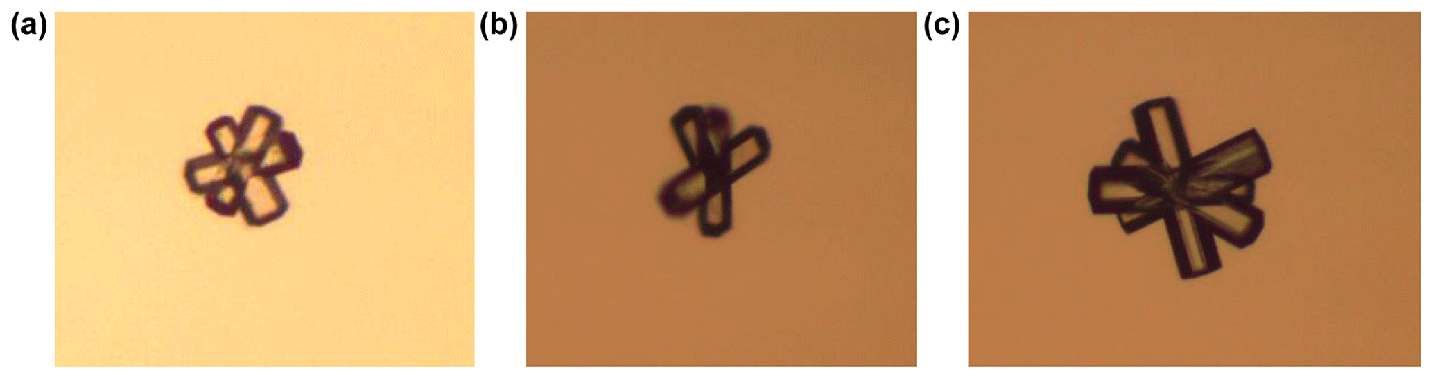
Figure 1Microscope images of sodium fluorosilicate crystals that were used as analogues for ice crystals. These are referred to as ROS118 (a), ROS250 (b), and ROS300 (c).
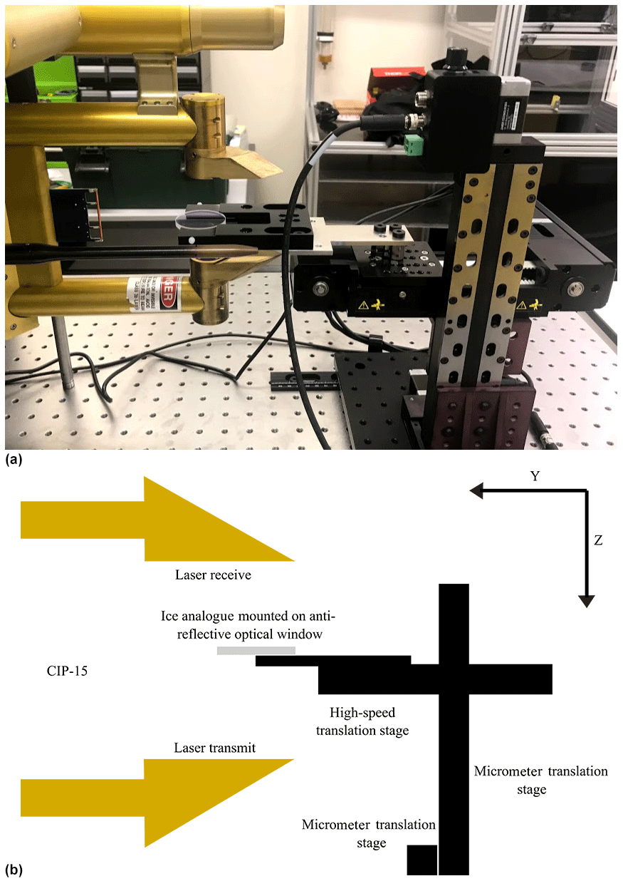
Figure 2(a) Image of the experimental set-up for the ice crystal analogue tests of the CIP-15. Panel (b) shows a schematic of the experimental set-up. The CIP-15 is horizontally mounted on the left of the image. The translation stages used to move ice crystal analogues through the CIP-15 sample volume are shown on the right of the image. The x axis is perpendicular to the plane of drawing.
CIP-15 images of the ice crystal analogues were collected by moving them through the laser beam along the axis of airflow. For each analogue, this was repeated five times before its position was stepped in 0.5 mm increments between the probe's vertical arms (along the z axis). This allows images of the analogues to be compared at different distances from the object plane.
Images were post-processed to take account of any difference in velocity between the stage and the CIP-15 data acquisition rate by resampling the images along the axis perpendicular to the optical array. This was performed to match the aspect ratio at Z = 0 of the CIP-15 image and a microscope image of each analogue. This typically corresponded to a particle stage velocity of ∼ 0.1 m s−1.
2.3 Synthetic data (angular spectrum theory)
Theoretical shadow images of 2D non-spherical shapes were calculated using a diffraction model based on angular spectrum theory (referred to as the AST model). Several previous studies describe this model in detail (Vaillant de Guélis et al., 2019a, b). We initialised the model using a 2D binary image of an opaque shape at the object plane (Z = 0) and calculated the wave field for different positions between the probe arms in the z axis. This model has been shown to give good agreement with OAP images of several types of 2D rectangular columns using images printed on a rotating disc (Vaillant de Guélis et al., 2019a).
In this study, we use a variety of different shapes to initialise the model. In Sect. 3.1, the diffraction model is compared to CIP15 images of 3D ice crystal analogues. To initialise the model for the comparisons with ROS250 and ROS300, the CIP-15 image of them at Z = 0 is used. Due to the smaller size of ROS118 and coarse pixel size of the CIP-15, a microscope image of the analogue is used to initialise the model. This image was converted to a binary image.
In Sect. 3.2 the quality of OAP images of commonly occurring ice crystal habits is explored. This is done by initialising the model with a variety of different ice crystal images. The ice crystal dataset contains 1060 images that were collected using a cloud particle imager (CPI, SPEC Inc., USA) and has previously been used to train habit recognition algorithms (Lindqvist et al., 2012; O'Shea et al., 2016). It includes images of ice crystals from arctic, mid-latitude, and tropical clouds. These images have been manually classified into seven habits (rosette, column/bullet, plate, quasi-spherical, column aggregate, rosette aggregate, and plate aggregate). To initialise the model, each CPI image was converted to a binary image. Shadow images were calculated every 2 mm for the range Z = 0 to 100 mm. These images were averaged to 10 µm pixel resolution, which is typical of modern OAPs. All simulations were performed using a light wavelength of 0.658 µm.
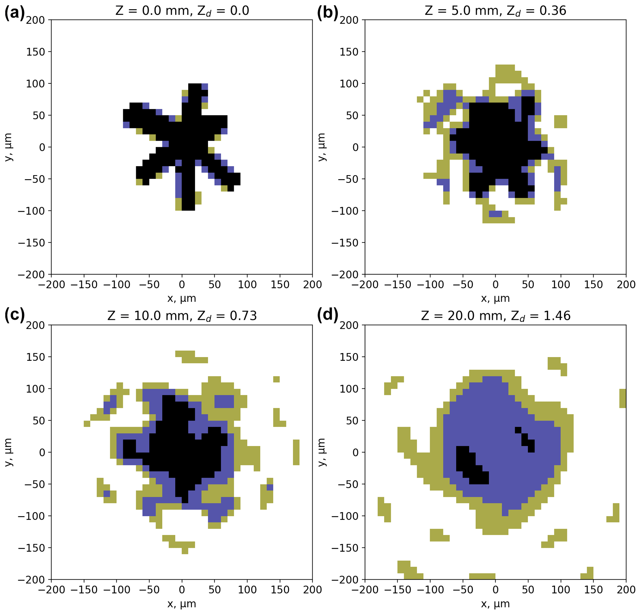
Figure 3Diffraction simulations from an image of a rosette crystal collected in cirrus cloud using a CPI (see text for details). Panel (a) shows the image at Z = 0 that is used to initialise the model. The other panels show images at different distances from the object plane (Z = 5, 10, and 20 mm). Green, blue, and black pixels correspond to decreases in detector intensity of 25 % to 50 %, 50 % to 75 %, and greater than 75 %, respectively.
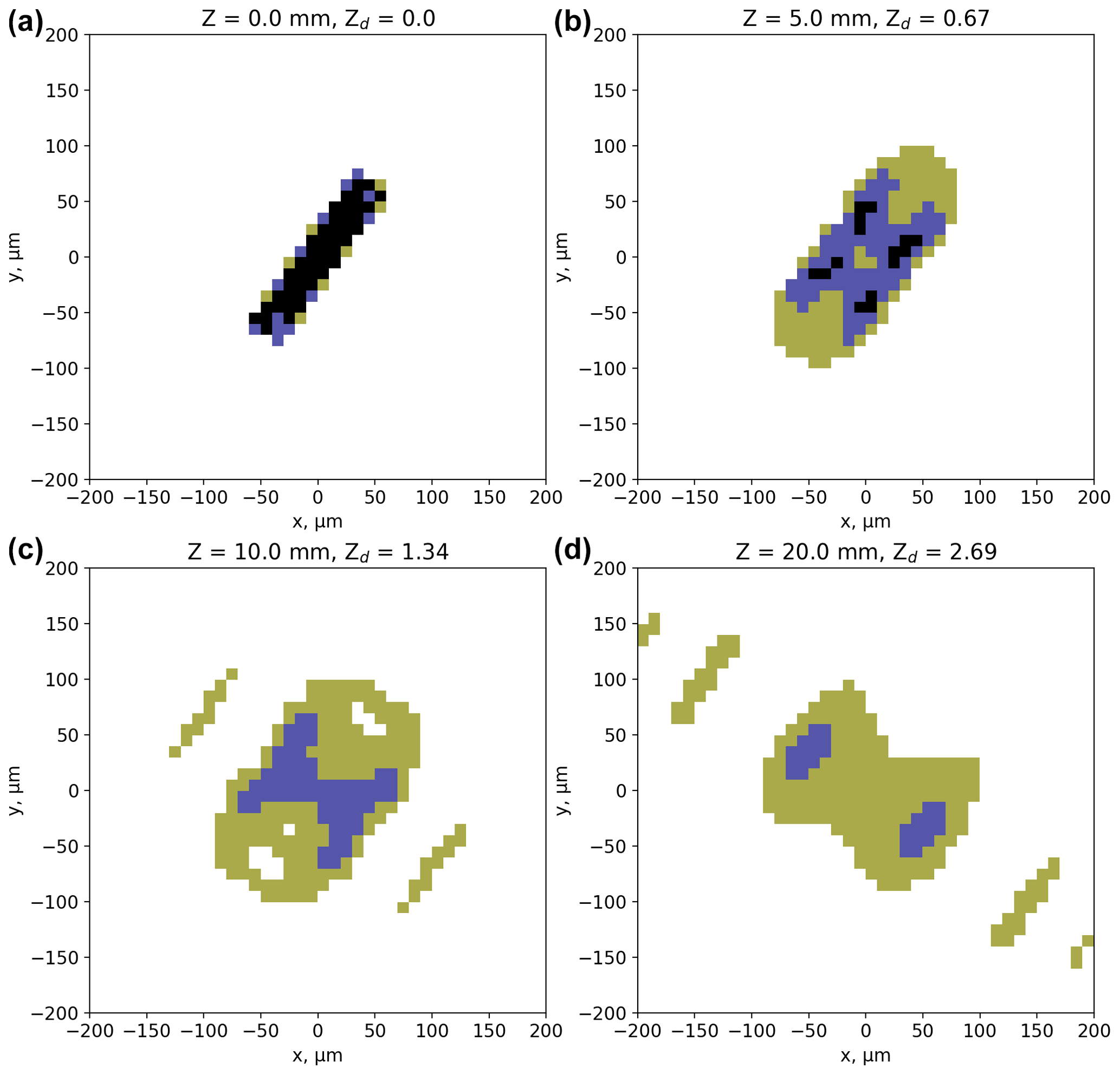
An example simulation for a rosette crystal is shown in Fig. 3 and a column in Fig. 4; the top left panels show the images at Z = 0 that are used to initialise the model. The other panels show images of the crystals at different distances from the object plane. Green, blue, and black pixels correspond to decreases in detector intensity of 25 % to 50 %, 50 % to 75 %, and > 75 %, respectively. Figures 3 and 4 show the rapid deterioration in image quality within a few millimetres of the object plane, which will impact derived properties such as particle size, number, and habit. This compares to many tens of millimetres for the typical arm separation of modern OAPs.
2.4 Aircraft measurements
This paper uses measurements from three flights by the Facility for Airborne Atmospheric Measurements (FAAM) BAe-146 research aircraft sampling frontal cirrus in the UK on the 11 March 2015 (nominal flight number B895), 7 February 2018 (C078), and 23 April 2018 (C097). The first two flights have previously been described in detail by O'Shea et al. (2016) and O19. For all three flights, the aircraft performed straight and level runs of approximately 10 min at different temperatures within the cloud. Ice crystals were dominated by rosettes, columns, and aggregates. Data from a 2D-S is available for the 11 March 2015 and CIP-15 for 7 February and 23 April 2018. On all flights the FAAM BAe-146 was fitted with a holographic imaging probe (HALOHolo). HALOHolo has a 6576 × 4384 pixel CCD (charged-coupled device) detector with an effective pixel size of 2.95 µm and arm separation of 155 mm. The probe acquires six frames per second, which equates to a volume sample rate of ∼ 230 cm3 s−1. The detection of small particles is limited by noise in the background image. Therefore, a minimum size threshold of 35 µm is applied, above which it is estimated that the probe's detection rate is greater than 90 % (Schlenczek, 2017). Shattered particles were minimised by removing all particles with interparticle distances less than 10 mm (Fugal and Shaw, 2009; O'Shea et al., 2016).
Section 4.2 shows a comparison between the 2D-S and a cloud droplet probe (CDP, DMT Inc.) during a flight in liquid stratus on 17 August 2018 (C031). The CDP sizes particles (3 to 50 µm) using the scattered light intensity assuming Mie scattering theory and spherical particles (Lance et al., 2010). The probe was calibrated during the campaign using glass spheres.
3.1 OAP and AST model comparison using ice crystal analogues
This section compares CIP-15 images of ice crystal analogues with diffraction simulations using the AST model. Figures 5–7 show the image size of the ice crystal analogues ROS118, ROS250, and ROS300 at different distances (Z) from the object plane measured by the CIP-15 (black markers) and modelled using angular spectrum theory (red lines). Top left panels show the image diameter (mean X–Y), while the particle area is shown in the top right; both use a 50 % drop in light intensity for the detection threshold. The other panels show different combinations of simple greyscale ratios. The abbreviations A25–50, A50–75, and A75–100 are used to denote the number of pixels associated with a decrease in detector signal of 25 %–50 %, 50 %–75 %, and 75 %–100 %, respectively. Example CIP-15 images of the ice crystal analogue ROS300 at three distance from the object plane are shown in Fig. 8.
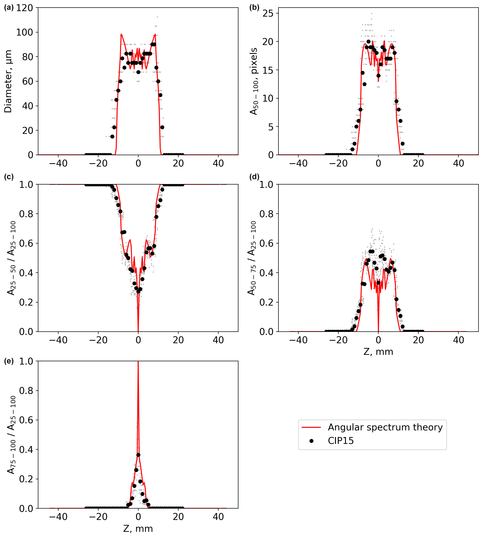
Figure 5A comparison between CIP-15 images and diffraction simulations (red lines) of the ice crystal analogue ROS118. Grey dots show data from individual CIP-15 images, and black dots show the median for each 1 mm Z bin. Panel (a) shows the mean X–Y image diameter. Panel (b) shows the number of pixels using 50 % detection thresholds. Other panels show the ratio of the number of pixels (area) at different greyscale thresholds.

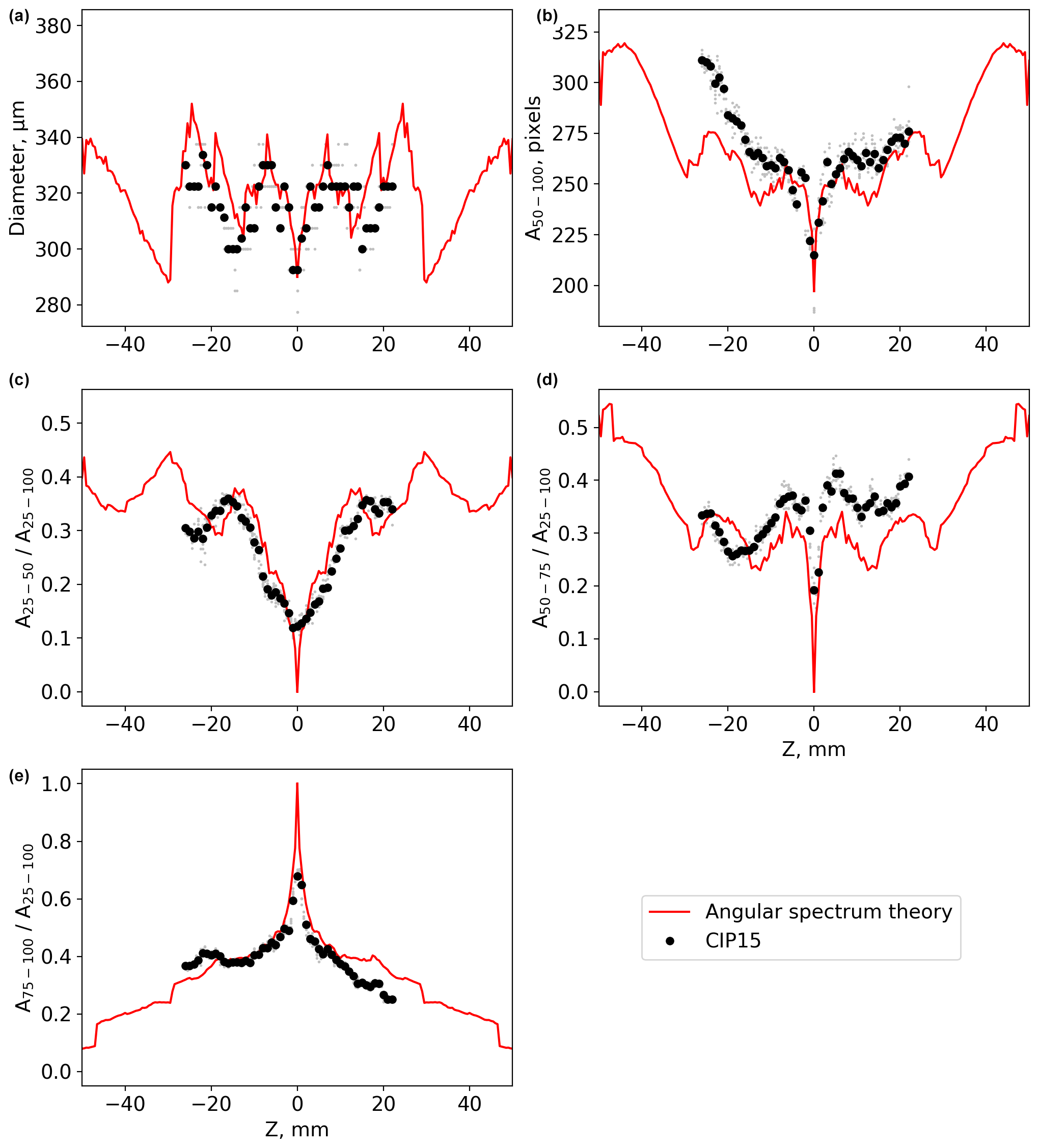
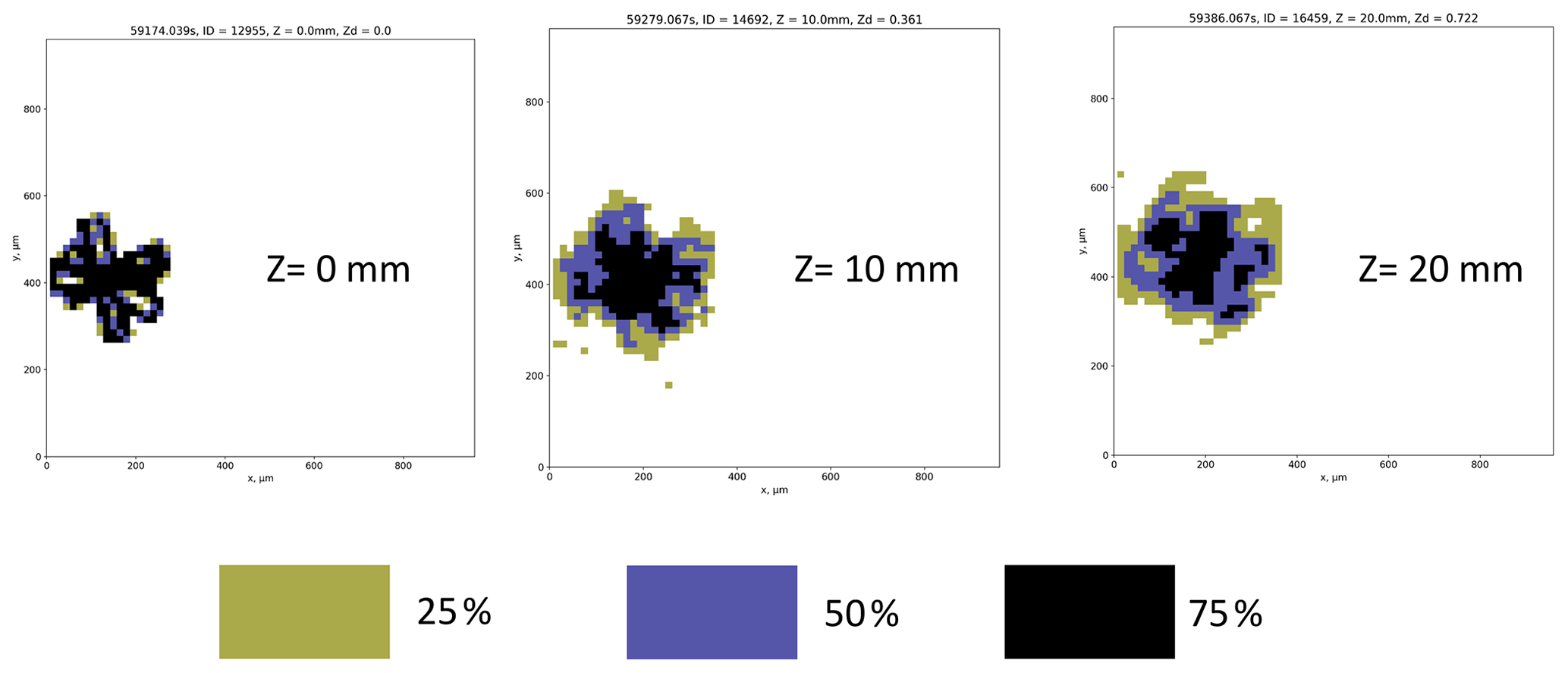
Figure 8CIP-15 images of the ice crystal analogue ROS300 at three distances from the object plane.
All three analogues have a general trend of diameter initially increasing with Z. The full DoF was sampled for ROS118 and shows the images fragmenting and diameter decreasing near the edge of the DoF. In addition to these general trends, there is a significant amount of fine-scale structure that is specific to each sample. There is a general trend of the greyscale ratio A75–100 decreasing with Z, while both A25–50 and A50–75 initially increase for all three analogues. Like the diameter vs. Z plots, there is a significant amount of fine-scale structure overlaying these general trends.
In general, the AST model can capture the large-scale structure in these measured parameters, although some discrepancies are present in the finer detail. For ROS118, the DoF from the experiments and the model agree to within ±1 mm (Fig. 5). The size and greyscale parameters calculated from CIP-15 images are not completely symmetrical about Z = 0. The reason for this is unclear; potential causes are if the CIP-15 laser beam is not perfectly collimated, additional refraction caused by the optical window used to mount the sample, or changes to the CIP-15 background or dark current calculation due to attenuation by the optical window.
3.2 OAP ice crystal sizing
Having investigated the performance of the AST model using 3D analogues of complex ice, we will now use the AST model to examine the ability of OAPs to correctly determine the size of commonly occurring ice crystals. Figure 9 left panels show the ratio of the measured diameter (D) to the true diameter (D0) vs. Zd for diffraction simulations of 1060 ice crystals. The data for each individual ice crystal are shown as grey lines, while the coloured lines are the median for each habit. Top panels show plots using the circle equivalent diameter, while the middle panels use the mean X–Y diameter and maximum diameter. Right panels show histograms of for each habit calculated for the Zd range from 0 to 10.
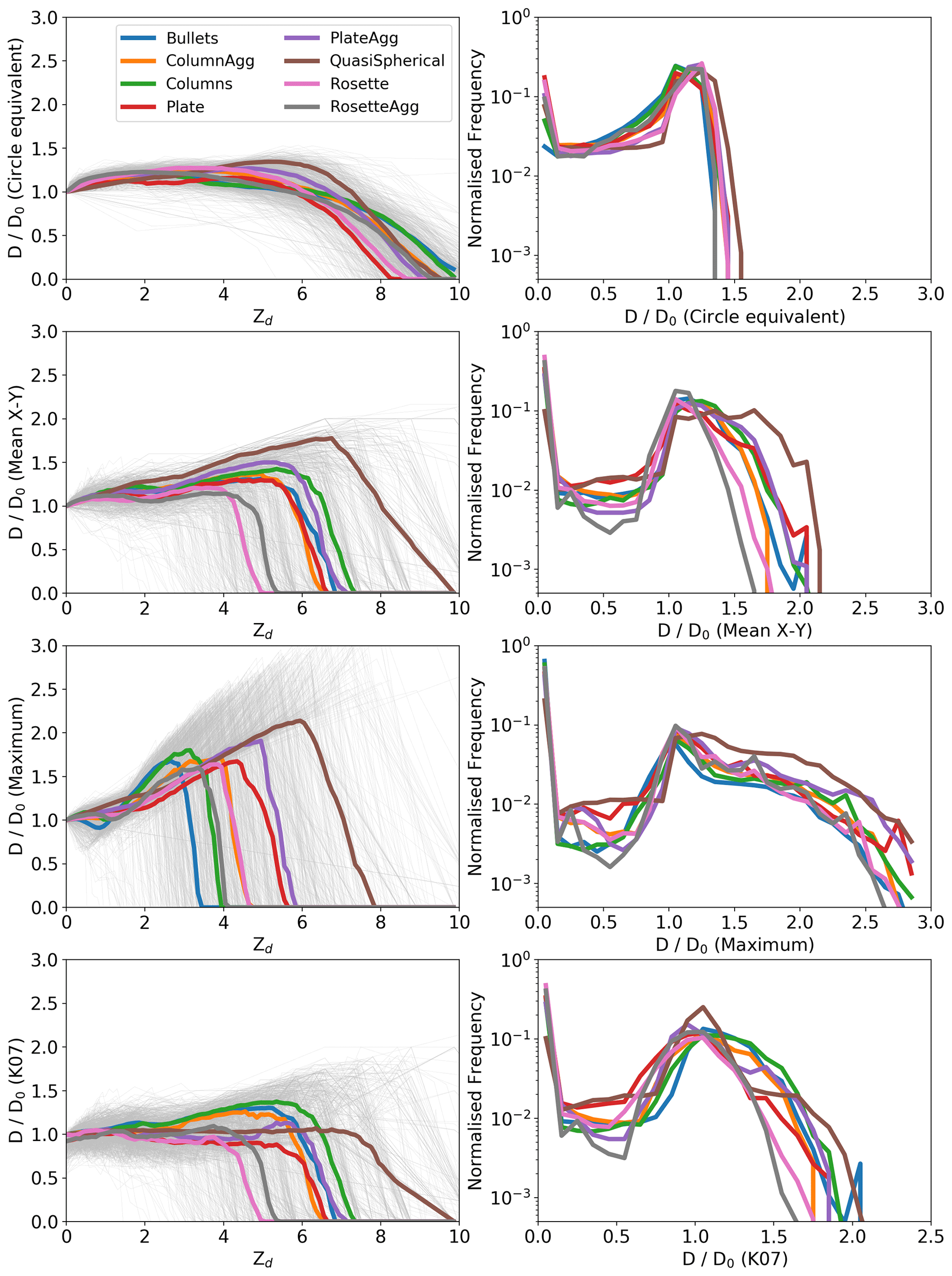
Figure 9Left panels show the ratio of the measured diameter (D) to the true diameter (D0) vs. Zd for diffraction simulations of 1060 ice crystals. The data for each individual ice crystal are shown as grey lines, while the coloured lines are the median for each habit. Right panels show histograms of for each habit calculated for the Zd range 0 to 10. Top panels show plots using the circle equivalent diameter, while the middle panels use the mean X–Y and maximum diameters. Bottom panels show the diameter corrected using K07.
Figure 9 shows large differences in these relationships depending on whether the mean X–Y, maximum, or circle equivalent diameters are used to define the particle size. For the 1060 ice crystal images used in this study, the median over the Zd range from 0 to 8 is 1.1 using circle equivalent diameter, 1.0 using the mean X–Y diameter, and 1.0 using the maximum diameter. However, there is significantly less variability between crystals using circle equivalent diameter, which has an interquartile range of 0.2 compared to 1.1 and 1.3 using the mean X–Y and maximum diameters, respectively. This is also shown in Tables S1–S3 in the Supplement, which gives the median and interquartile range at selected Zd for each habit using the three different size metrics.
There is a general trend of increasing size with distance from the object plane. Oversized estimations are up to approximately 100 %, 200 %, and 50 % using mean X–Y, maximum, and circle equivalent diameters, respectively. However, the degree of oversizing is dependent on habit, with quasi-spherical and plate aggregates most significantly oversized using all D definitions. In agreement with O19, once D reaches a maximum, further increases in Z cause the images to fragment and their size to decrease until they are no longer visible.
K07 use the size of the internal voids within images of droplets to determine their Zd and correct their size. O19 show that this algorithm is effective using modern OAPs for droplets with Zd < ∼ 6. For Zd > 6, the images are too fragmented for their size to be corrected. The K07 approach was derived by considering Fresnel diffraction from opaque discs and has only been tested for images of spherical droplets. However, in the absence of an alternative, previous studies have applied K07 to images of ice crystals (e.g. Davis et al., 2010). To examine the efficacy of this approach, Fig. 9 bottom panels show the mean X–Y diameter of the simulated images of ice crystals once the K07 approach has been applied. The ratio of their K07 corrected diameter to their true particle diameter is shown as a function of Zd (left panel), while probability density functions of for each habit are shown in the right panel. The median for the Zd range 0 to 8 is 0.9, and the interquartile range is 1.1. For a number of habits (rosette, plate, quasi-spherical, rosette aggregate, and plate aggregate), K07 reduce the number of oversized particles across most of the DoF. For bullets, columns, and column aggregates, the K07 approach has minimal impact on the probe sizing. For all habits, the K07 approach is not able to remove the small image fragments that occur when a particle is near the edge of the DoF.
3.3 Depth of field dependence on particle habit
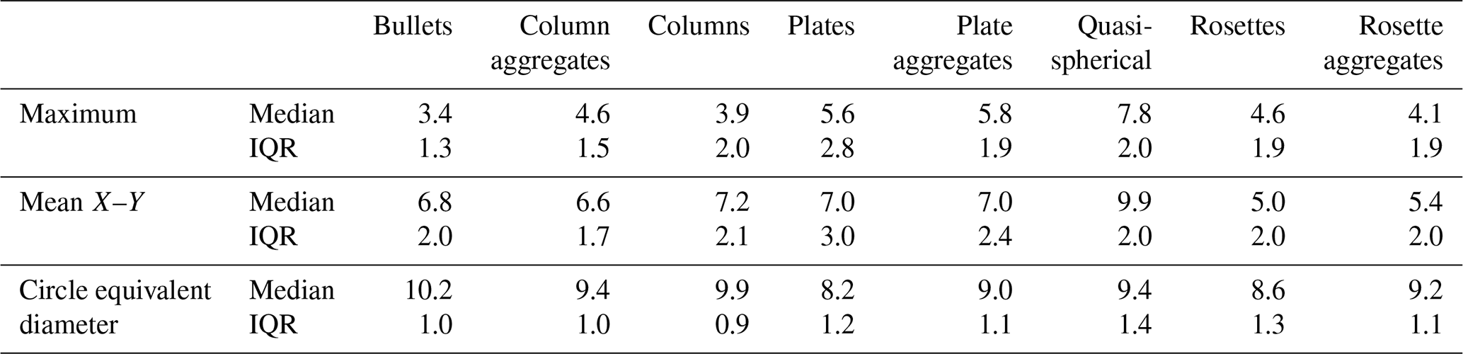
Uncertainty of derived physical quantities (e.g. number concentration) from OAPs is dependent on the sample volume and therefore uncertainty in the DoF (see Eq. 2). The DoF of an OAP is commonly calculated using Eq. (1) with a single c value. The variable c in this equation is the Zd where a particle is no longer detected by the OAP. If a single c value is used this would need to be independent of particle shape. Table 1 shows the median and interquartile range Zd where particles are no longer visible for each habit using the maximum, mean X–Y and circle equivalent diameters. Using mean X–Y, the habit median DoF varies between Zd = 5.0 and 9.9 for rosettes and quasi-spherical particles, respectively. Using the maximum as the particle sizing metric, the median DoF varies by a similar amount ranging between Zd = 3.4 and 7.8 for bullets and quasi-spherical crystals. In addition, particles have significant intra-habit variability using both maximum and mean X–Y, with most habits DoF interquartile ranges greater than 2 Zd. The variability is lower using circle equivalent diameter, with median DoFs ranging between 8.2 and 10.2 for plates and bullets, respectively, with habit interquartile ranges near 1 Zd. As a result, derived physical quantities such as number concentration will have lower uncertainty if circle equivalent diameter is used to define the particle size compared to maximum and mean X–Y diameters.
Table 1Median and interquartile range (IQR) normalised dimensionless distance from the object plane (Zd) where particles are no longer visible for different habits; this is equivalent to c in Eq. (1).
3.4 Greyscale information
Greyscale information in OAP imagery has previously been used to filter severely mis-sized images and enforce a DoF threshold that improves data quality (O19). Figure 10 shows combinations of simple greyscale ratios as a function of Zd for the simulation of 1060 ice crystal images described in the previous section. Left panels use the size metric mean X–Y diameter in the Zd calculation, whereas the right panels use circle equivalent diameter in the Zd calculation. Like the ratio (Fig. 9), the greyscale ratios also show significant variability between habits as a function of Zd. Figure 10 shows this variability is greater if mean X–Y diameter is used to calculate Zd, although it is still significant using circle equivalent diameter. The variability is larger still using maximum diameter (not shown).
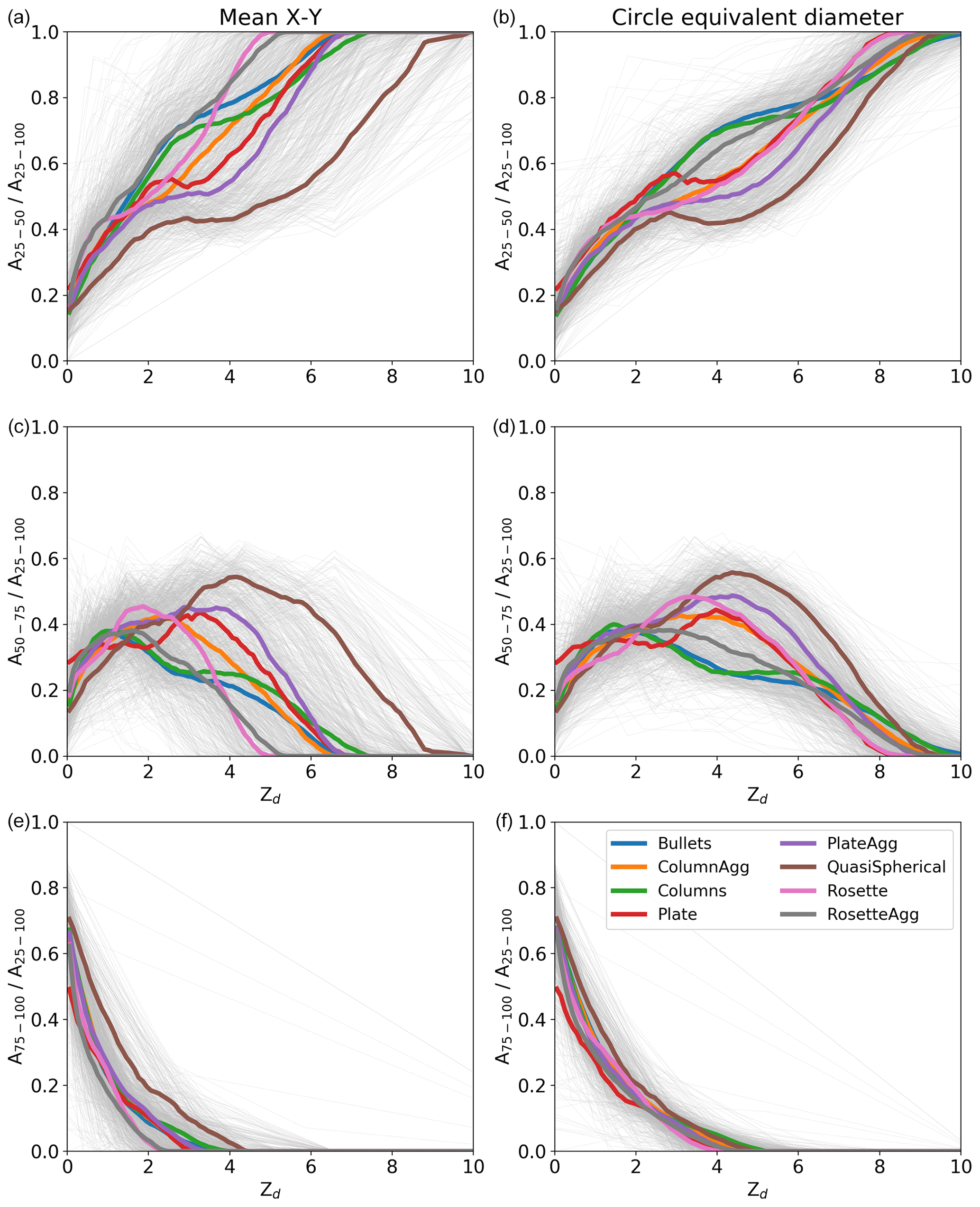
Figure 10Combinations of number of pixels at different greyscale ratios as a function of Zd for the simulated ice crystal images. Panels (a), (c), and (e) show plots where mean X–Y is used as the sizing metric, while panels (b), (d), and (f) use circle equivalent diameter.
The O19 approach uses simple greyscale ratios to determine Zd for spherical liquid droplets near the edge of the DoF (3.5 < Zd < 8.5). This allows a new DoF to be defined that excludes fragmented images, removing significant biases in the PSD. This is possible since all spherical droplets independent of size have the same greyscale ratios at a given Zd. Figure 10 shows that this is not true for ice crystals where the initial shape of the ice crystal has an impact on the greyscale ratios at a given Zd. As a result, the O19 approach cannot be used to determine Zd in the same way.
3.5 Habit recognition
The shape of ice crystals is a key microphysical parameter impacting cloud radiative properties in several ways. A variety of automatic image recognition algorithms have been applied to OAP datasets to classify particles into different habits (Korolev and Sussman, 2000; Crosier et al., 2011; Praz et al., 2018). These algorithms typically rely on geometrical features extracted from OAP images that have characteristic values for specific habits. These characteristic values are usually determined by manually classifying images into habits. These images are then used to set thresholds or train machine learning algorithms to automatically classify new images. For example, Crosier et al. (2011) used the following ratio to discriminate between ice crystals and liquid droplets:
where P is the particle perimeter, and A is the particle area including any internal void. Crosier et al. (2011) used a threshold of 1.25 to discriminate between these two categories. When images are manually selected to train habit recognition algorithms, only images that can be identified “by eye” as a specific habit will be included. For OAPs this is likely to be images that are “in focus”. However, the shape of an OAP image and therefore the geometrical features that are used in habit recognition algorithms depend on where in the probe's sample volume a particle is detected. For example, Fig. 3 shows a simulated 190 µm rosette at different distances from the object plane. It is only in the top left panel (Z = 0) that it can be identified as a rosette from its image alone. Figure 11 shows how this particle's circularity changes with Z and Zd. At Z = 0 its circularity is near 4, while at Z = 20 mm it is near 1 and may be confused with a spherical droplet. Figure 11 demonstrates that the measured particle shape is highly dependent on the position in the sample volume Zd (and Z) with the circularity decreasing by a factor 2 by Zd = 1; in comparison the particle size has only changed by 15 %.
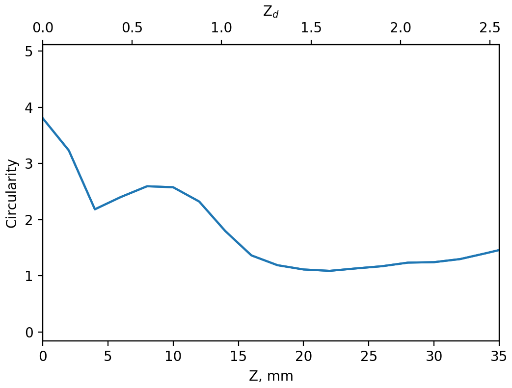
Figure 11The circularity (Eq. 4) of the rosette shown in Fig. 3 as a function of distance from the object plane Z and Zd.
The variance in geometrical features for each habit will not only be due to natural variability in the shape of ice crystals but also due to their position in the sample volume when measured. To date, this second effect has not been accounted for by habit recognition algorithms. Therefore, currently the results of habit classification algorithms on OAP datasets cannot be considered quantitative.
Depending on where in the sample volume a particle is observed, the OAP image size can range between being as small as a single pixel and up to twice the true particle diameter (see Fig. 9). Algorithms such as those in K07 and O19 have been derived using spherical shapes and are therefore not directly applicable to OAP PSDs of non-spherical shapes. However, there are several possible approaches that could be used to correct OAP ice crystal size distributions.
4.1 Greyscale filtering
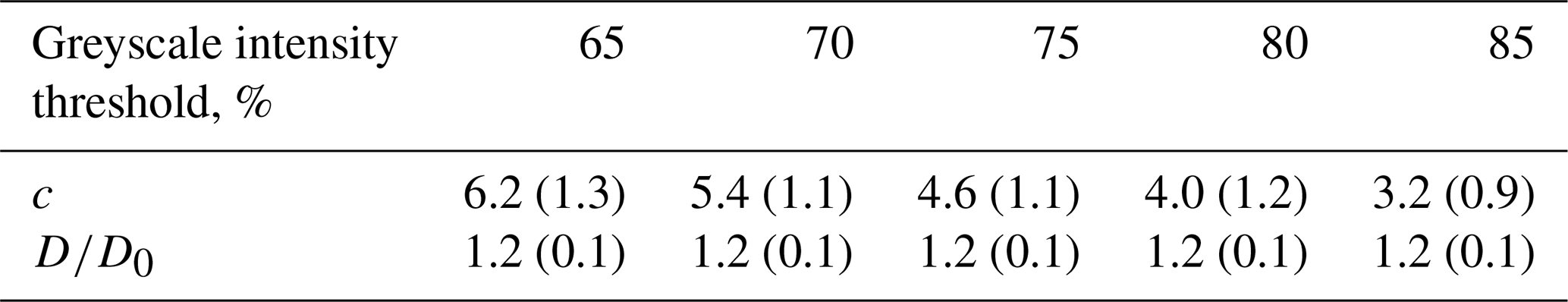
Unlike for liquid droplets, the O19 approach does not accurately determine Zd for non-spherical ice crystals. We now describe a new technique to use greyscale information to remove the most severely mis-sized ice crystals and constrain the sample volume with a reasonable uncertainty using circle equivalent diameter as the particle sizing metric. For example, if the diffraction simulations are filtered to only include images that have at least one pixel with a greater than a 75 % drop in light intensity (Fig. 7), then the median position where particles are no longer visible (using a 50 % intensity threshold) is Zd = 4.6 (interquartile range 1.1 in Zd). This removes the fragmented images that begin to occur at approximately 6. The median ratio for Zd < 4.6 is 1.2 (interquartile range = 0.1); however, particles may still be oversized by approximately 40 % even with this filter applied (Fig. 7). Other greyscale thresholds may be used to provide a more or less restrictive DoF constraint. Table 2 shows the median (interquartile range) c values for various greyscale thresholds between 65 % and 85 %. Using a 65 % threshold the median c value is 6.2 (interquartile range = 1.3), while for 85 % it is 3.2 (interquartile range = 0.9). It should be noted that the lower the greyscale threshold, the higher the probability of a fragmented image being observed and the small particle concentration being biased.
Table 2Median (interquartile range) depth of field c value (Eq. 1) for 1060 ice crystal images using various greyscale intensity thresholds and circle equivalent diameter. The median (interquartile range) ratio for Zd < c is also given.
When determining the effective array width (Eq. 2), the image size along the direction of the photodiode array should be used. However, this size is a function of the particle's Z position, which is the reason why the effective array width needs to be integrated over the depth of field to determine the sample volume (Eq. 2). This can be calculated using the AST model if the true particle shape can be assumed (e.g. spherical particles in liquid cloud). However, if the true particle shape is not known, as is often the case for ice clouds, then it remains a source of uncertainty in the calculated sample volume.
Figures 12 and 13 apply this new methodology to ambient measurements collected during research flights in cirrus on 7 February and 23 April 2018. Figure 12 shows PSDs from the CIP-15 and HALOHolo for a run at −42 ∘C on 7 February 2018 (16:02:00 to 16:10:00 GMT). This flight has previously been discussed by O19. Figure 13 shows equivalent PSDs for temperatures between −47 and −40 ∘C collected on 23 April 2018. For both probes, the particle diameter given is the circle equivalent diameter, and particles in contact with the edge of the CIP-15 optical array have not been included in the PSD calculation. The black lines show the CIP-15 size distribution when images are filtered to only include those with at least one pixel at the 75 % intensity threshold. This threshold significantly reduces the concentration of small particles (< 200 µm) compared to when this filtering is not applied (grey lines) and generally is in much better agreement with HALOHolo (a holographic imaging probe) (blue markers). This suggests that for these cases using current data-processing techniques, a significant fraction of the ice crystal number concentration at sizes < 200 µm is an artefact due to optical effects.

Figure 12Size distributions from the CIP-15 and HALOHolo for a run at −42 ∘C on 7 February 2018. The black line shows the CIP-15 size distribution when images are filtered to only include those with at least one pixel at the 75 % intensity threshold.
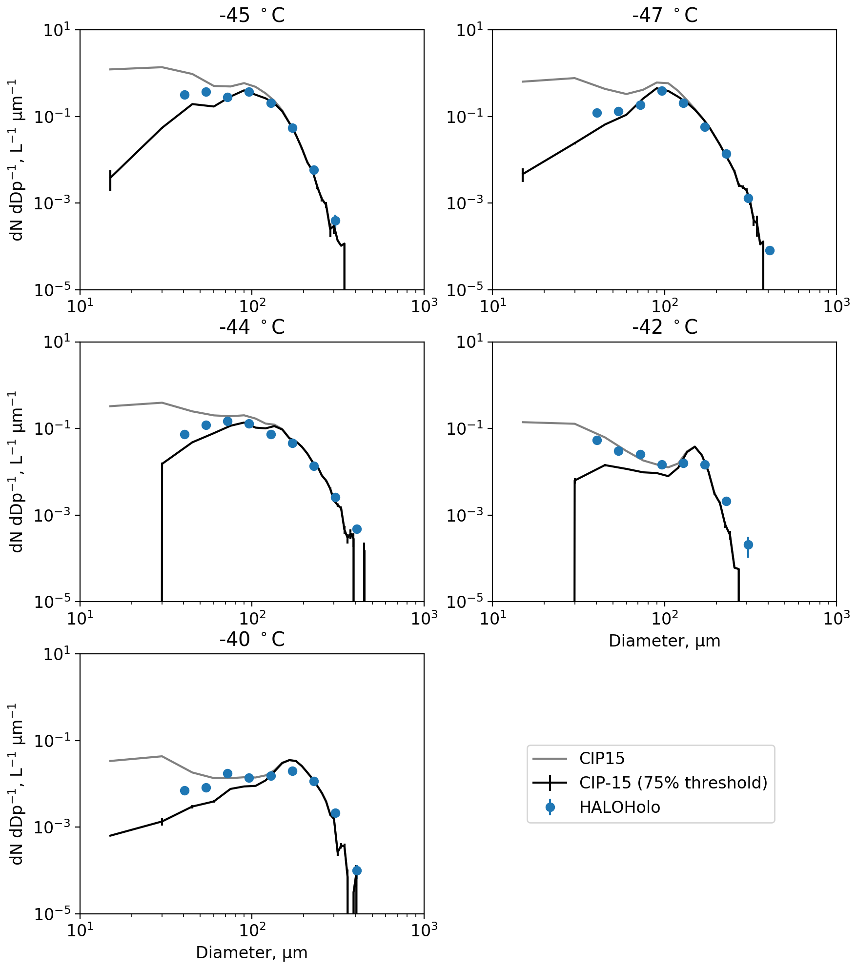
Figure 13Size distributions from the CIP-15 and HALOHolo for runs between −47 and −40 ∘C on 23 April 2018. The black line shows the CIP-15 size distribution when images are filtered to only include those with at least one pixel at the 75 % intensity threshold.
HALOHolo's sample volume is not as strongly dependent on particle size as it is for OAPs. However, as described earlier, measurements of small particles from HALOHolo are limited by noise in the background image. For a complete description of the HALOHolo data-processing and quality-control procedures, see Schlenczek (2017). HALOHolo uses supervised machine learning to discriminate real particles from artefacts due to noise in the background image. However, it is possible that small particles could be misclassified as artefacts or vice versa, and as a result HALOHolo could either underestimate or overestimate the small ice concentration. For particles > 35 µm, it is estimated that the probe's detection rate is > 90 %, and previous work has shown excellent agreement with a CDP in liquid clouds (Schlenczek, 2017). However, HALOHolo PSDs should not be considered the true PSD but rather another piece of evidence that suggests for these cases OAPs overestimate small ice concentrations using current data-processing techniques.
4.2 Stereoscopic imaging
A second method that could be used to constrain the DoF of an OAP is to use the stereoscopic imaging that is possible with the 2D-S. The 2D-S in effect consists of two OAPs (known as channels) orientated perpendicular to each other and the direction of motion of the particle and instrument. Under normal operation the probe is oriented so that one laser beam is horizontal and the other is vertical. The two lasers overlap at the centre of each channel's arms. As well as increasing sampling statistics by having two channels which can be merged or averaged, this design also allows some ice crystals to be viewed from two orientations to study their aspect ratios. In this study we use this feature to constrain the probe's DoF, which greatly limits the magnitude of diffraction artefacts and represents the first implementation of stereoscopic analysis on an ambient OAP dataset. The 2D-S was designed so that Z = 0 on both channels is in the region where the two lasers overlap. We refer to particles observed by both channels as co-located particles. Co-located particles have tightly constrained Z position and should not be subject to significant mis-sizing due to diffraction. For the 2D-S, this is likely to be true for D0 > 20 µm. For a hypothetical stereoscopic probe with larger optical arrays, it may be necessary to restrict the distance a particle can be from the centre of the optical array.
For the case where channel 0 is used for particle sizing and channel 1 is used to constrain the particle Z position, the sample volume of co-located particles is given by
where TAS is the true air speed, E is the number of array elements, R is the resolution of the probe, D is the measured particle diameter, and DCH0 is the particle diameter measured along the axes of the channel 0 optical array. This requires that particles in contact with the edge of the channel 0 optical array have been removed. If channel 1 is used for particle sizing instead of channel 0, then particles in contact with the edge of the channel 1 optical array are removed instead of channel 0, and DCH0 is replaced by DCH1 in Eq. (5).
For this method to be applicable, it is important to validate that Z = 0 on both channels is in the laser overlap region. If it is significantly offset this would prevent small co-located particles from being observed, since the DoF from one channel would not overlap with the optical array of the other channel. Increasingly large offsets between the channels prevent increasingly large co-located particles from being observed. It is therefore important to check that this offset is not significant by regularly sampling in environments where small particles are present (i.e. in liquid cloud or using a droplet generator in a laboratory as in O19).
Co-located particles could be confused with shattered particles since they are also associated with short inter-arrival times. Figure 14 (top panel) shows a histogram of inter-arrival time for particles on the same channel for measurements in cirrus on 7 February 2018. To minimise shattering events, each channel was independently filtered for particles using an inter-arrival threshold of 1 × 10⁻⁵ s. It may still be possible to mistakenly detect shattered particles as co-located particles if one shattering fragment splits into two particles, triggering each channel simultaneously but in spatially independent parts of the sample volume. However, examination of co-located images suggest that this is rare.
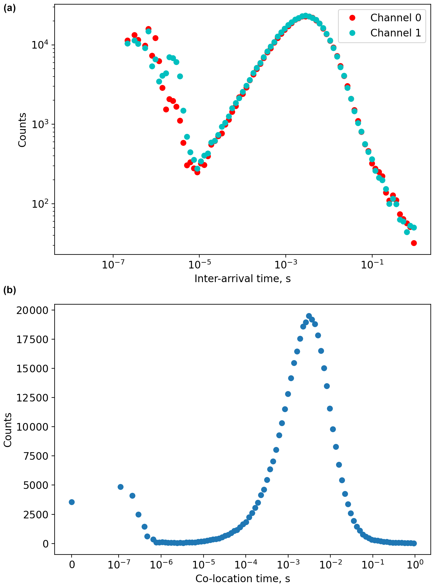
Figure 14(a) Histograms of inter-arrival times for particles on the same 2D-S channel for measurements in cirrus on 7 February 2018. (b) A histogram of the difference in arrival time between a particle on one channel and their closest neighbour on the other channel.
To identify co-located particles, we use the difference in arrival time between a particle on one channel and their closest neighbour on the other channel. Figure 14 shows a histogram of co-location times for measurements in cirrus on 7 February 2018. This distribution is bimodal with a larger mode centred at approximately 1 × 10⁻³ s and a smaller mode at 1 × 10⁻⁷ s. The larger mode is associated with the typical spatial separation between ambient particles, with its position dependent on the particle concentration. Examining pairs of images from the smaller mode suggests that these images are the same ice crystal viewed from different orientations. Figure 15 shows example pairs of co-located images, with channel 0 images shown in yellow and channel 1 images shown in blue. In addition to overall consistency in the geometrical shapes between channel 0 and channel 1 images, there is also excellent consistency in the particle size along the airspeed direction (x axis in Fig. 15) between these two channels.

Figure 15Example ice crystals observed by both channels of the 2D-S. Images from channel 0 are shown in yellow and images from channel 1 are shown in blue.
Figure 14 shows that most co-located particles do not trigger both channels simultaneously within the time resolution of the data acquisition system but are offset by a few hundred nanoseconds. At 100 m s−1 data slices from the detectors are acquired every 1 × 10⁻⁷ s, which corresponds to a spatial separation of 10 µm. Using the laboratory droplet generator system described in O19, we were able to generate a continuous stream of droplets of known size, velocity, rate, and with precise control over the position within the sample volume. These experiments with particle velocities of 1 m s−1 resulted in a 1 × 10⁻⁵ s mode time delay in detection events between the two channels of the 2D-S. This also corresponds to an offset of 10 µm in the sample volume in the axis of airflow through the probe (y axis). These two sets of analysis provide a robust independent verification of the spatial offset between the two channels of the 2D-S. Therefore, when considering ambient data, we classify co-located particles as those with time separations less than 5 × 10⁻⁷ s.
Figure 16 shows a comparison between PSDs collected in liquid stratus cloud at 13 ∘C on 17 August 2018. The grey lines show the 2D-S data for each channel using conventional data-processing protocols without constraining the DoF, while the green and red lines show PSDs for just the co-located particles. The CDP is shown in blue. For this case, no particles larger than approximately 200 µm are present. All data-processing methods are in good agreement up to 100 µm. For larger sizes, the measurements using the co-located particles are limited by counting statistics due to the low concentration of these particles. This illustrates the ability of the 2D-S to detect small co-located particles.
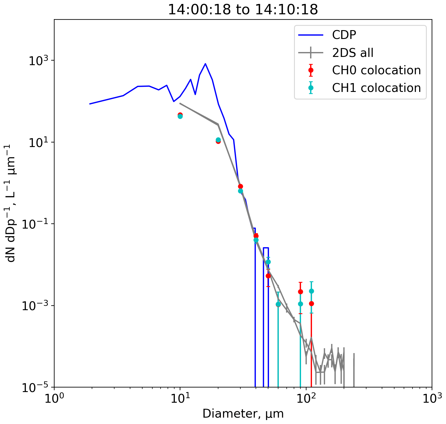
Figure 16Size distributions from the 2D-S and CDP for different temperatures during a research flight in liquid stratus on 17 August 2018 at 13 ∘C. The grey lines show the 2D-S data using conventional data-processing protocols without constraining the DoF, while the green and red lines show size distributions for just the co-located particles. CDP size distributions are shown in blue.

Figure 17Size distributions from the 2D-S and HALOHolo for different temperatures during a research flight in cirrus on 11 March 2015. The grey lines show the 2D-S data using conventional data-processing protocols without constraining the DoF, while the green and red lines show size distributions for just the co-located particles. The dashed black line shows a 2D-S processed using a hybrid of conventional and co-location data processing (see text for details). HALOHolo size distributions are shown in blue.
Figure 17 shows size distributions from the 2D-S and HALOHolo for different temperatures (averaged over ∼ 10 min) during a research flight in cirrus on 11 March 2015 (see O'Shea et al., 2016). The grey lines show the 2D-S data for each channel using conventional data-processing protocols without constraining the DoF, while the red lines show size distributions for just the co-located particles. HALOHolo size distributions are shown in blue. For all temperatures, the conventional 2D-S data processing shows an ice crystal mode at small sizes (< 200 µm). At warmer temperatures (> −39 ∘C) there is also a clear second mode at larger sizes. However, these high concentrations of small ice particles are not present in the co-located and the HALOHolo size distributions. This suggests that using only co-located particles on the dual channel 2D-S probe is effective at removing significant biases at small particle sizes. At larger sizes (> 300 µm) the 2D-S data processing using conventional and stereoscopic methods are in good agreement; however, the latter method is limited by sampling statistics.
Stereoscopic data processing has the advantage of removing out-of-focus artefacts that bias the PSD at small sizes, while at larger sizes traditional processing methods offer significantly improved sampling statistics. Therefore, a hybrid approach using stereoscopic processing for small sizes and traditional processing methods for larger sizes is advantageous. The choice of size threshold to switch between the two methods is dependent on the arm width of the probe and the level of mis-sizing that is deemed acceptable. To give an idea of a suitable threshold, we will choose a size limit that prevents all particles with Zd > 2 from being included in the PSD. The maximum Z that the 2D-S can observe a particle is Z = 31.5 mm (2D-S arm_width/2). This corresponds to a 222 µm particle at Zd = 2. However, since particles can be mis-sized by a factor 1.4, a size threshold of 300 µm is needed to ensure that no particle with Zd > 2 is included. Figure 17 (dashed lines) shows 2D-S PSDs processed using this hybrid approach.
4.3 Other potential methods
There are several other potential methods that could be used to improve OAP PSD measurements. First, reducing a probe's arm width to physically limit a distance a particle can be from the object plane would reduce out-of-focus particles. The amount the arm width would need to be decreased depends on the level of mis-sizing that is deemed acceptable for a given particle size, with more accurate sizing and smaller particles requiring smaller arm widths. However, as well as decreasing the sample volume, reducing the probe's arm width is likely to increase the proportion of shattered artefact particles compared to ambient particles that the probe measures, since shattered artefacts are thought to cluster near the probe's arms.
Second, statistical retrievals have been applied to particle size distribution measurements where the instrument response is a distorted version of the true ambient distribution. These methods are reliant on knowing or empirically approximating the instrument function that distorts the ambient distribution. These methods have been applied to OAP measurements of spherical droplets (Korolev et al., 1998; Jensen and Granek, 2002). For non-spherical particles, the distortion function is dependent on the ice crystal habits present; therefore, the derived size distributions would have greater uncertainty, unless the particle shape is known a priori. However, this methodology may still result in an acceptable level of uncertainty if circle equivalent diameter is used, since its intra- and inter-habit (Zd) variance is smaller than for the mean X–Y and maximum diameters.
In situ measurements of ice clouds have consistently observed a mode in particle size distributions at small sizes (< 200 µm). This would imply that ice nucleation occurs at all cloud levels, since small ice particles would rapidly grow in regions of ice supersaturation or sublime in sub-saturated regions. Particle shattering on the leading edge of a probe has previously been identified as a possible explanation (Korolev and Isaac, 2005; Korolev et al., 2011). However, the impacts of shattering are thought to have been minimised by modifying the leading edges of probes (Korolev et al., 2013) and using particle inter-arrival time algorithms (Field et al., 2006; Korolev and Field, 2015). Yet even with these improved measurements a small ice mode has been found to be ubiquitous in ice cloud observations (McFarquhar et al., 2007; Jensen et al., 2009; Cotton et al., 2013; Jackson et al., 2015; O'Shea et al., 2016).
This work has shown that depending on where in the OAP sample volume a particle is observed its image size can be as small as a single pixel or up to a 200 % overestimate of the true particle diameter (see Fig. 9). Only a relatively small proportion of undersized larger particles are required to generate a significant bias in number concentration at small sizes (< 200 µm) due to the size dependence of the DoF (Eq. 1) (O19). We have tested two methods that could be used to remove out-of-focus artefacts: greyscale filtering (Sect. 4.1) and stereoscopic imaging (Sect. 4.2). Both methods either remove or significantly reduce the concentration of small ice crystals observed in specific cirrus cloud cases (Figs. 12, 13 and 17).
To further explore the impact OAP mis-sizing has on the measured PSD shape, we use the results from the AST model. Consider the ambient ice crystal PSD N(D0) with units L−1 µm−1. N(D0) is a 1-D array with E elements (the number of array elements). If this distribution is observed by an OAP with size-dependent sample volume SVol(D0) (units: L−1 s−1, Eq. 2), then the number of ice crystals observed by the probe as a function of true particle diameter C(D0) (units: µm−1 s−1) is given by
SVol(D0) and C(D0) are both 1-D arrays with E elements. The symbol ⊙ denotes Hadamard (element-wise) multiplication. The number of ice crystals observed as a function of the measured diameter C(D) is given by
where M(D,D0) is an E×E array. Each column of M(D,D0) is the probability distribution that a particle of true size D0 has measured size D. These probabilities are dependent on the particle shape, the particle sizing metric, probe characteristics (e.g. arm width, laser wavelength), and the data-processing protocols used (e.g. greyscale filtering, co-location). The PSD observed by the probe N(D) (1-D array with E elements) can then calculated by
The symbol ⊘ denotes Hadamard (element-wise) division. The probe arm width limits the maximum Zd that a particle of given D0 can be observed. By choosing an arm width, it is possible to calculate a probability distribution function of possible D for each D0 from one of the (Zd) relationships shown in Fig. 9. For our example, we use an arm width of 70 mm and the median relationship for rosettes. We calculate M(D,D0) for two cases: when mean X–Y and circle equivalent diameters are used as the particle sizing metric. To represent the true ambient distribution, we use three different gamma distributions that all have the form
where N is the number concentration. Figure 18 shows three combinations of the coefficients μ, λ (cm−1), and N0 (L−1 cm−1). Left panels show plots using mean X–Y diameter and the right panels show plots using circle equivalent diameter. The ambient PSDs (blue lines) are compared to simulated OAP observations using different data-processing methodologies. The grey lines represent an OAP with arm width of 70 mm using conventional data-processing methods. The red markers represent a 2D-S using only co-located particles, which has the effect of limiting the maximum Z a particle can be observed at to 0.64 mm. The blue markers show simulated OAP measurements from a greyscale probe with 70 mm arm width when the data have been filtered to only include particles that have at least one pixel with a greater than 75 % decrease in light intensity.

Figure 18Simulations of OAP measurements of different gamma PSDs (blue lines). The coefficients μ, λ (cm−1), and N0 (L−1 cm−1) for each gamma PSD are shown in text boxes. Panels (a), (c), and (e) show plots using mean X–Y diameter and panels (b), (d), and (f) show circle equivalent diameter. The grey lines show simulated OAP PSDs with arm width of 70 mm if all the particles are rosettes. The red markers show simulated 2D-S measurements using only co-located particles, which has the effect of limiting the maximum Z a particle can be observed at to 0.64 mm. The blue markers show simulated OAP measurements from a greyscale probe with 70 mm arm width when the data have been filtered to only include particles that have at least one pixel with a greater than 75 % decrease in light intensity.
It should be noted that these simulated distributions only include mis-sizing due to diffraction and do not include other sources of OAP measurement uncertainty (e.g. counting statistics). Counting statistics will be responsible for a larger uncertainty for the co-located PSDs compared to conventional data-processing methods.
Figure 18 top panels show an ambient distribution (blue lines) dominated by small particles (μ = −1, λ = 1000 cm−1, and N0 = 10 L−1 cm−1), with concentrations increasing with decreasing size over the displayed size range 10 to 1280 µm, which is representative of modern OAPs. The grey lines show the simulated OAP observations of this PSD, which have a similar characteristic shape. The total particle concentration observed by the simulated OAP over the size range 10 to 1280 µm is 3 % and 13 % higher than the true PSD using mean X–Y and circle equivalent diameters, respectively. Figure 18 top left panel shows the PSD that a 2D-S would observe when only co-located particles are included (red markers). The total particle concentration from the co-located PSD differs from the ambient distribution by less than 1 %. The total particle concentration when greyscale filtering is applied is 2 % lower that the true distribution.
Figure 18 middle panels show an ambient distribution with mode near 100 µm particles (μ = 2, λ = 200 cm−1, and N0 = 1 × 10⁴ L−1 cm−1). The simulated OAP PSDs have significantly different shapes with much higher concentrations of particles < 100 µm. Here the OAP overestimates the total particle concentration over the size range 10 to 1280 µm by 74 % and 80 % using mean X–Y and circle equivalent diameters, respectively. When stereoscopic imaging is used to constrain the OAP sample volume (red lines), the small particle mode is removed. The true and simulated OAP total particle concentration differ by < 1 %. Greyscale filtering again removes the small particle mode but underestimates the total particle concentration by 11 %.
Figure 18 bottom panels show an ambient PSD with mode near 400 µm particles (μ = 4, λ = 100 cm−1, and N0 = 1 × 10⁶ L−1 cm−1); like the previous case the simulated OAP PSD significantly overestimates the small particle concentration. The simulated OAP PSD is bi-modal, while the true PSD is mono-modal. However, in this case the artificial small particles contribute a relatively small proportion to the total number concentration in the 10 to 1280 µm size range; as a result the simulated OAP only overestimates this by 4 % using both particle size metrics.
A significant amount of our understanding of cloud microphysics is based on OAP measurements, with the small particle artefact being present and manifesting in some manner. This includes how PSDs are parameterised in numerical models and remote sensing retrievals. Generally in the literature some formulation of exponential or gamma function has been used to represent ice crystal PSDs for observation or modelling studies (e.g. Cazenave et al., 2019; Delanoë et al., 2005, 2014; Field et al., 2007; Heymsfield et al., 2013; McFarquhar and Heymsfield, 1997). These functions and the coefficients that are used in the literature all result in the highest ice crystal concentrations at the smallest sizes. For example, Field et al. (2007) describe a parameterisation based on OAP measurements that is widely used by the passive and active remote sensing communities (e.g. Mitchell et al., 2018; Sourdeval et al., 2018; Ekelund et al., 2020; Eriksson et al., 2020; Fontaine et al., 2020). It describes a characteristic ice crystal PSD that can be used to calculate moments of a PSD when the ice water content is known. The functional form of the parameterisation consists of the summation of a gamma and exponential distribution.
Figure 19 shows a comparison between the 2D-S PSD for 11 March 2015 and the Field et al. (2007) parameterisations for tropical (Eq. 10) and mid-latitude (Eq. 11) ice clouds.
where the number concentration (N(D)) and diameter are normalised using the second (M2) and third (M3) moments of the PSD, and x is equal to . The 2D-S PSD in Fig. 19 has been calculated using only co-located particles for D < 300 µm and all particles for D > 300 µm. Both the tropical and mid-latitude parameterisations show rapidly increasing concentrations with decreasing size. At larger sizes the 2D-S and these parameterisations are in good agreement, while they diverge at smaller sizes. The green line in Fig. 19 shows the gamma component of the mid-latitude F07 parameterisation (Eq. 12), which is in much better agreement with the observations at small sizes.
This work suggests that the data used for derived PSDs parameterisations are subject to significant artefacts. As a result, the parameterisations are likely to have incorrect fundamental shape for ice cloud PSDs. The impacts of these artefacts can be expected to propagate to inaccuracies in remote sensing retrievals, which will be assimilated into weather forecast models, and to incorrect radiative properties due to a bias towards small particle sizes. Future work is needed to quantify the impact on retrievals and our understanding of ice microphysics and cloud radiative properties using the improved measurement methodologies presented in this paper.
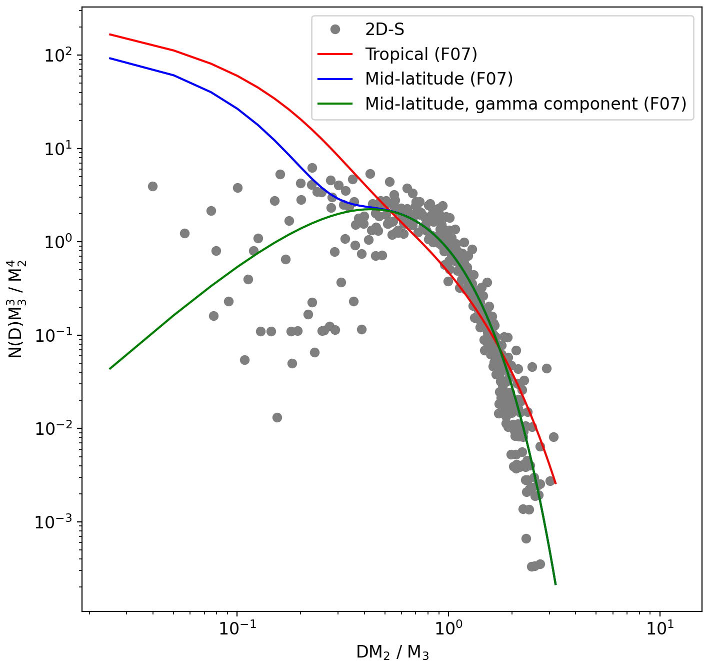
Figure 19Comparison between 2D-S size distributions of co-located particles from a research flight in cirrus on 11 March 2015 and Field et al. (2007) parameterisations for tropical and mid-latitude ice clouds.
This paper quantifies the optical response of OAPs to non-spherical particles for understanding ice crystal observations, expanding the work of O19. We make the following comments and recommendations on the use of OAP data:
-
The shape and size of an OAP image depends significantly on where in the OAP sample volume a particle is observed. Particles < 200 µm are the most significantly mis-sized. The measured size of a particle can range between being as small as a single pixel up to being as large as a 200 % overestimate of the true particle.
-
Particle mis-sizing and the size dependence of the OAP sample volume cause an artefact which results in systematic overestimate of small ice (< 200 µm) concentrations. The persistent mode of small sizes observed in many previously studied cases is likely artificial. However, the importance of this artefact is strongly influenced by the true shape of the ambient PSD.
-
Algorithms to correct OAP size distributions such as those in K07 and O19 that have been derived using spherical particles are not applicable to non-spherical ice crystal images without significant uncertainty.
-
New methods that may be used to filter OAP ice crystal size distributions were tested, including filtering using greyscale and the use of stereoscopic imaging.
-
For greyscale instruments (such as the CIP-15), filtering images so that they must include one pixel with at least a 75 % decrease in detector intensity removes the most severely fragmented particles near the edge of the DoF. This approach constrains the DoF to c = 4.6 (interquartile range 1.1) using circle equivalent diameter.
-
Using the stereoscopic imaging that is possible with the 2D-S can constrain the sample volume to only in-focus images. A hybrid approach using stereoscopic processing for small sizes and traditional processing methods for larger sizes is advantageous, as it limits any negative impacts on sample volume and therefore counting statistics. The choice of size threshold to switch between the two methods is dependent on the arm width of the probe and the level of mis-sizing that is deemed acceptable. For the 2D-S, we suggest that 300 µm is a suitable threshold for particle sizing using the mean X–Y diameter.
-
These new methodologies were tested using data from three research flights sampling cirrus. In these cases, they significantly improved agreement with a holographic imaging probe compared to conventional data-processing protocols and either removed or significantly reduced the concentration mode at small particle sizes (< 200 µm). This raises questions over the interpretation of many existing datasets such as those used to parameterise PSDs (e.g. Delanoë et al., 2005, 2014; Field et al., 2007) and the persistent observation of small particles throughout the entire vertical extent of ice clouds, which has been difficult to reconcile with concepts of ice nucleation.
-
Past datasets from OAPs need to be revisited, and where possible the filtering and sample volume adjustments described in this paper should be applied. The impact these corrections have on how PSDs are parameterised in numerical models, remote sensing retrievals, and radiative calculations of ice clouds needs to be examined.
The data presented here can be provided on request to the contact author.
The supplement related to this article is available online at: https://doi.org/10.5194/amt-14-1917-2021-supplement.
SO'S, JC, JD, LG, and ZU performed laboratory experiments. SO'S, JC, JD, WS, KB, OS, RC, and CW collected and/or processed airborne measurements. SO'S performed model experiments. SB provided and supported the use of the holographic probe. SO'S and JC analysed and interpreted the data. SO'S wrote the paper. All authors commented on and/or edited the paper.
The authors declare that they have no conflict of interest.
We would like to thank Thibault Vaillant de Guélis for his help with the AST model. We are grateful to Jacob Fugal for assistance with HALOHolo. The authors wish to thank Hannakaisa Lindqvist (CSU) for making her CPI training dataset available. Airborne data were obtained using the BAe-146-301 Atmospheric Research Aircraft (ARA) flown by Directflight Ltd and managed by the Facility for Airborne Atmospheric Measurements (FAAM), which is a joint entity of the Natural Environment Research Council (NERC) and the Met Office. The CIP-15 instruments were provided by the National Centre for Atmospheric Science and FAAM. The National Centre for Atmospheric Science provided support for the ice crystal analogue experiments.
This research has been supported by NERC (grant nos. NE/P012426/1 and NE/L013584/1).
This paper was edited by Szymon Malinowski and reviewed by two anonymous referees.
Baumgardner, D. and Korolev, A.: Airspeed Corrections for Optical Array Probe Sample Volumes, J. Atmos. Ocean. Tech., 14, 1224–1229, https://doi.org/10.1175/1520-0426(1997)014<1224:ACFOAP>2.0.CO;2, 1997.
Baumgardner, D., Jonsson, H., Dawson, W., O'Connor, D., and Newton, R.: The cloud, aerosol and precipitation spectrometer: a new instrument for cloud investigations, Atmos. Res., 59–60, 251–264, https://doi.org/10.1016/S0169-8095(01)00119-3, 2001.
Cazenave, Q., Ceccaldi, M., Delanoë, J., Pelon, J., Groß, S., and Heymsfield, A.: Evolution of DARDAR-CLOUD ice cloud retrievals: new parameters and impacts on the retrieved microphysical properties, Atmos. Meas. Tech., 12, 2819–2835, https://doi.org/10.5194/amt-12-2819-2019, 2019.
Cotton, R. J., Field, P. R., Ulanowski, Z., Kaye, P. H., Hirst, E., Greenaway, R. S., Crawford, I., Crosier, J., and Dorsey, J.: The effective density of small ice particles obtained from in situ aircraft observations of mid-latitude cirrus, Q. J. Roy. Meteor. Soc., 139, 1923–1934, 2013.
Crosier, J., Bower, K. N., Choularton, T. W., Westbrook, C. D., Connolly, P. J., Cui, Z. Q., Crawford, I. P., Capes, G. L., Coe, H., Dorsey, J. R., Williams, P. I., Illingworth, A. J., Gallagher, M. W., and Blyth, A. M.: Observations of ice multiplication in a weakly convective cell embedded in supercooled mid-level stratus, Atmos. Chem. Phys., 11, 257–273, https://doi.org/10.5194/acp-11-257-2011, 2011.
Davis, S., Hlavka, D., Jensen, E., Rosenlof, K., Yang, Q., Schmidt, S., Borrmann, S., Frey, W., Lawson, P., Voemel, H., and Voemel, T. P.: In situ and lidar observations of tropopause subvisible cirrus clouds during TC4, J. Geophys. Res.-Atmos., 115, D00J17, https://doi.org/10.1029/2009JD013093, 2010.
Delanoë, J., Protat, A., Testud, J., Bouniol, D., Heymsfield, A. J., Bansemer, A., Brown, P. R. A., and Forbes, R. M.: Statistical properties of the normalized ice particle size distribution, J. Geophys. Res., 110, D10201, https://doi.org/10.1029/2004JD005405, 2005.
Delanoë, J. M. E., Heymsfield, A. J., Protat, A., Bansemer, A., and Hogan, R. J.: Normalized particle size distribution for remote sensing application, J. Geophys. Res.-Atmos., 119, 4204–4227, https://doi.org/10.1002/2013JD020700, 2014.
Ekelund, R., Eriksson, P., and Pfreundschuh, S.: Using passive and active observations at microwave and sub-millimetre wavelengths to constrain ice particle models, Atmos. Meas. Tech., 13, 501–520, https://doi.org/10.5194/amt-13-501-2020, 2020.
Eriksson, P., Rydberg, B., Mattioli, V., Thoss, A., Accadia, C., Klein, U., and Buehler, S. A.: Towards an operational Ice Cloud Imager (ICI) retrieval product, Atmos. Meas. Tech., 13, 53–71, https://doi.org/10.5194/amt-13-53-2020, 2020.
Field, P. R., Heymsfield, A. J., and Bansemer, A.: Shattering and Particle Interarrival Times Measured by Optical Array Probes in Ice Clouds, J. Atmos. Ocean. Tech., 23, 1357–1371, 2006.
Field, P. R., Heymsfield, A. J., and Bansemer, A.: Snow Size Distribution Parameterization for Midlatitude and Tropical Ice Clouds, J. Atmos. Sci., 64, 4346–4365, https://doi.org/10.1175/2007JAS2344.1, 2007.
Fontaine, E., Schwarzenboeck, A., Leroy, D., Delanoë, J., Protat, A., Dezitter, F., Strapp, J. W., and Lilie, L. E.: Statistical analysis of ice microphysical properties in tropical mesoscale convective systems derived from cloud radar and in situ microphysical observations, Atmos. Chem. Phys., 20, 3503–3553, https://doi.org/10.5194/acp-20-3503-2020, 2020.
Fugal, J. P. and Shaw, R. A.: Cloud particle size distributions measured with an airborne digital in-line holographic instrument, Atmos. Meas. Tech., 2, 259–271, https://doi.org/10.5194/amt-2-259-2009, 2009.
Gurganus, C. and Lawson, P.: Laboratory and flight tests of 2D imaging probes: Toward a better understanding of instrument performance and the impact on archived data, J. Atmos. Ocean. Tech., 35, 1533–1553, https://doi.org/10.1175/JTECH-D-17-0202.1, 2018.
Heymsfield, A. J., Schmitt, C., and Bansemer, A.: Ice cloud particle size distributions and pressure dependent terminal velocities from in situ observations at temperatures from 0 to −86 ∘C, J. Atmos. Sci., 70, 4123–4154, 2013.
Jackson, R. C., McFarquhar, G. M., Fridlind, A. M., and Atlas, R.: The dependence of cirrus gamma size distributions expressed as volumes in Nµ phase space and bulk cloud properties on environmental conditions: Results from the Small Ice Particles in Cirrus Experiment (SPARTICUS), J. Geophys. Res.-Atmos., 120, 10351–10377, https://doi.org/10.1002/2015JD023492, 2015.
Jensen, E. J., Lawson, P., Baker, B., Pilson, B., Mo, Q., Heymsfield, A. J., Bansemer, A., Bui, T. P., McGill, M., Hlavka, D., Heymsfield, G., Platnick, S., Arnold, G. T., and Tanelli, S.: On the importance of small ice crystals in tropical anvil cirrus, Atmos. Chem. Phys., 9, 5519–5537, https://doi.org/10.5194/acp-9-5519-2009, 2009.
Jensen, J. B. and Granek, H.: Optoelectronic Simulation of the PMS 260X Optical Array Probe and Application to Drizzle in a Marine Stratocumulus, J. Atmos. Ocean. Tech., 19, 568–585, https://doi.org/10.1175/1520-0426(2002)019<0568:OSOTPO>2.0.CO;2, 2002.
Knollenberg, R. G.: The optical array: An alternative to scattering or extinction for airborne particle size determination, J. Appl. Meteorol., 9, 86–103, https://doi.org/10.1175/1520-0450(1970)009<0086:TOAAAT>2.0.CO;2, 1970.
Korolev, A.: Reconstruction of the sizes of spherical particles from their shadow images, Part I: Theoretical considerations, J. Atmos. Ocean. Tech., 24, 376–389, 2007.
Korolev, A. and Field, P. R.: Assessment of the performance of the inter-arrival time algorithm to identify ice shattering artifacts in cloud particle probe measurements, Atmos. Meas. Tech., 8, 761–777, https://doi.org/10.5194/amt-8-761-2015, 2015.
Korolev, A. and Isaac, G. A.: Shattering during sampling by OAPs and HVPS, Part 1: Snow particles, J. Atmos. Ocean. Tech., 22, 528–542, https://doi.org/10.1175/JTECH1720.1, 2005.
Korolev, A. and Sussman, B.: A technique for habit classification of cloud particles, J. Atmos. Ocean. Tech., 17, 1048–1057, 2000.
Korolev, A., Emery, E., and Creelman, K.: Modification and Tests of Particle Probe Tips to Mitigate Effects of Ice Shattering, J. Atmos. Ocean. Tech., 30, 690–708, https://doi.org/10.1175/JTECH-D-12-00142.1, 2013.
Korolev, A. V., Kuznetsov, S. V., Makarov, Y. E., and Novikov, V. S.: Evaluation of measurements of particle size and sample area from optical array probes, J. Atmos. Ocean. Tech., 8, 514–522, 1991.
Korolev, A. V., Strapp, J. W., and Isaac, G. A.: Evaluation of the accuracy of PMS optical array probes, J. Atmos. Ocean. Tech., 15, 708–720, https://doi.org/10.1175/1520-0426(1998)015<0708:EOTAOP>2.0.CO;2, 1998.
Korolev, A. V., Emery, E. F., Strapp, J. W., Cober, S. G., Isaac, G. A., Wasey, M., and Marcotte, D.: Small ice particles in tropospheric clouds: Fact or artifact? Airborne icing instrumentation evaluation experiment, B. Am. Meteorol. Soc., 92, 967–973, https://doi.org/10.1175/2010BAMS3141.1, 2011.
Lance, S., Brock, C. A., Rogers, D., and Gordon, J. A.: Water droplet calibration of the Cloud Droplet Probe (CDP) and in-flight performance in liquid, ice and mixed-phase clouds during ARCPAC, Atmos. Meas. Tech., 3, 1683–1706, https://doi.org/10.5194/amt-3-1683-2010, 2010.
Lawson, R. P., O'Connor, D., Zmarzly, P., Weaver, K., Baker, B., Mo, Q., and Jonsson, H.: The 2D-S (stereo) probe: design and preliminary tests of a new airborne, high-speed, high-resolution particle imaging probe, J. Atmos. Ocean. Tech., 23, 1462–1477, https://doi.org/10.1175/JTECH1927.1, 2006.
Lindqvist, H., Muinonen, K., Nousiainen, T., Um, J., McFarquhar, G. M., Haapanala, P., Makkonen, R., and Hakkarainen, H.: Ice cloud particle habit classification using principal components, J. Geophys. Res., 117, D16206, https://doi.org/10.1029/2012JD017573, 2012.
McFarquhar, G. M. and Heymsfield, A. J.: Parameterization of tropical cirrus ice crystal size distributions and implications for radiative transfer: Results from CEPEX, J. Atmos. Sci., 54, 2187–2200, https://doi.org/10.1175/1520-0469(1997)054<2187:POTCIC>2.0.CO;2, 1997.
McFarquhar, G. M., Um, J., Freer, M., Baumgardner, D., Kok, G. L., and Mace, G.: The importance of small ice crystals to cirrus properties: Observations from the Tropical Warm Pool International cloud Experiment (TWP-ICE), Geophys. Res. Lett., 57, L13803, https://doi.org/10.1029/2007GL029865, 2007.
Mitchell, D. L., Garnier, A., Pelon, J., and Erfani, E.: CALIPSO (IIR–CALIOP) retrievals of cirrus cloud ice-particle concentrations, Atmos. Chem. Phys., 18, 17325–17354, https://doi.org/10.5194/acp-18-17325-2018, 2018.
O'Shea, S. J., Choularton, T. W., Lloyd, G., Crosier, J., Bower, K. N., Gallagher, M., Abel, S. J., Cotton, R. J., Brown, P. R. A., Fugal, J. P., Schlenczek, O., Borrmann, S., and Pickering, J. C.: Airborne observations of the microphysical structure of two contrasting cirrus clouds, J. Geophys. Res., 121, 13510–13536, https://doi.org/10.1002/2016JD025278, 2016.
O'Shea, S. J., Crosier, J., Dorsey, J., Schledewitz, W., Crawford, I., Borrmann, S., Cotton, R., and Bansemer, A.: Revisiting particle sizing using greyscale optical array probes: evaluation using laboratory experiments and synthetic data, Atmos. Meas. Tech., 12, 3067–3079, https://doi.org/10.5194/amt-12-3067-2019, 2019.
Praz, C., Ding, S., McFarquhar, G. M., and Berne, A.: A versatile method for ice particle habit classification using airborne imaging probe data, J. Geophys. Res., 123, 13472–13495, https://doi.org/10.1029/2018JD029163, 2018.
Schlenczek, O.: Airborne and ground-based holographic measurement of hydrometeors in liquid-phase, mixed-phase and ice clouds, PhD thesis, University of Mainz, Mainz, Germany, https://doi.org/10.25358/openscience-4124, 2017.
Sourdeval, O., Gryspeerdt, E., Krämer, M., Goren, T., Delanoë, J., Afchine, A., Hemmer, F., and Quaas, J.: Ice crystal number concentration estimates from lidar–radar satellite remote sensing – Part 1: Method and evaluation, Atmos. Chem. Phys., 18, 14327–14350, https://doi.org/10.5194/acp-18-14327-2018, 2018.
Ulanowski, Z., Hesse, E., Kaye, P. H., Baran, A. J., and Chandrasekhar, R.: Scattering of light from atmospheric ice analogues, J. Quant. Spectrosc. Ra., 79, 1091–1102, 2003.
Vaillant de Guélis, T., Schwarzenböck, A., Shcherbakov, V., Gourbeyre, C., Laurent, B., Dupuy, R., Coutris, P., and Duroure, C.: Study of the diffraction pattern of cloud particles and the respective responses of optical array probes, Atmos. Meas. Tech., 12, 2513–2529, https://doi.org/10.5194/amt-12-2513-2019, 2019a.
Vaillant de Guélis, T., Shcherbakov, V., and Schwarzenböck, A.: Diffraction patterns from opaque planar objects simulated with Maggi-Rubinowicz method and angular spectrum theory, Opt. Express, 27, 9372–9381, https://doi.org/10.1364/OE.27.009372, 2019b.
Wendisch, M. and Brenguier, J.-L.: Airborne Measurements for Environmental Research: Methods and Instruments, Wiley-VCH Verlag GmbH and Co. KGaA, Weinheim, Germany, ISBN 978-3-527-40996-9, 2013.