LiSBOA (LiDAR Statistical Barnes Objective Analysis) for optimal design of lidar scans and retrieval of wind statistics – Part 2: Applications to lidar measurements of wind turbine wakes

The LiDAR Statistical Barnes Objective Analysis (LiSBOA), presented in Letizia et al. (2021), is a procedure for the optimal design of lidar scans and calculations over a Cartesian grid of the statistical moments of the velocity field. Lidar data collected during a field campaign conducted at a wind farm in complex terrain are analyzed through LiSBOA for two different tests. For both case studies, LiSBOA is leveraged for the optimization of the azimuthal step of the lidar and the retrieval of the mean equivalent velocity and turbulence intensity fields. In the first case, the wake velocity statistics of four utility-scale turbines are reconstructed on a 3D grid, showing LiSBOA's ability to capture complex flow features, such as high-speed jets around the nacelle and the wake turbulent-shear layers. For the second case, the statistics of the wakes generated by four interacting turbines are calculated over a 2D Cartesian grid and compared to the measurements provided by the nacelle-mounted anemometers. Maximum discrepancies, as low as 3 % for the mean velocity (with respect to the free stream velocity) and turbulence intensity (in absolute terms), endorse the application of LiSBOA for lidar-based wind resource assessment and diagnostic surveys for wind farms.

1 Introduction

The use of Doppler light detection and ranging (lidar) technology for wind energy applications has largely increased over the last decade (Clifton et al., 2018; Veers et al., 2019). Thanks to the achieved measurement accuracy and simpler and cost-effective deployments compared to traditional meteorological tower instrumentation, this remote sensing technique is now included in the international standards as a reliable tool for performance diagnostics of wind turbines and wind resource assessments (International Electrotechnical Commission 61400-12-1, 2017). Nonetheless, due to the limited spatiotemporal resolution and the distribution of the sample points in a spherical reference frame, the reconstruction of wind statistics from lidar samples still presents several challenges (Sathe et al., 2011; Newman et al., 2016).

In the companion paper (Letizia et al., 2021), we presented a revisited Barnes objective analysis (Barnes, 1964) for the calculation of wind statistics from scattered lidar data, which is referred to as LiDAR Statistical Barnes Objective Analysis (LiSBOA). This procedure enables the estimation, over a Cartesian grid, of the mean, variance, and even higher-order central statistical moments of the radial velocity field probed by a scanning Doppler pulsed wind lidar. LiSBOA also performs adequate filtering of small-scale variability in the mean velocity field and mitigation of the dispersive stresses on the higher-order statistics, provided that the algorithm is tuned based on the characteristics of the flow under investigation and the free parameters of the lidar scan are optimally designed through LiSBOA.

LiSBOA's ability to estimate statistics of an ergodic turbulent velocity field makes it a suitable tool for the analysis of wind turbine wakes and the resource assessment of sites characterized by heterogeneous wind conditions, such as in presence of flow distortions induced by complex terrain. Over the last decade, wind lidars have been used to investigate wind turbine wakes; for instance, Käsler et al. (2010) and Clive et al. (2011) measured the velocity deficit past utility-scale wind turbines, while Bingöl et al. (2010) used a nacelle-mounted lidar to detect wake displacements and validate the dynamic wake meandering model (Larsen et al., 2008). Fitting of the wake velocity deficit was successfully exploited to extract quantitative information about wake evolution from lidar measurements (Aitken and Lundquist, 2014; Wang and Barthelmie, 2015; Kumer et al., 2015; Trujillo et al., 2016; Bodini et al., 2017).

A deeper understanding of the physics of turbine wakes was achieved by calculating temporal (Trujillo et al., 2011; Iungo et al., 2013b; Iungo and Porté-Agel, 2014; Kumer et al., 2015; Machefaux et al., 2015; Van Dooren et al., 2016) or conditional (Aubrun et al., 2016; Machefaux et al., 2016; Garcia et al., 2017; Bromm et al., 2018; Iungo et al., 2018; Zhan et al., 2019, 2020) statistics of the velocity collected through lidar scans performed at different times. Using this approach, Iungo and Porté-Agel (2014) detected a significant dependence of the wake recovery rate on atmospheric stability, based on time-averaged volumetric lidar scans. The same concept was expanded by other authors using ensemble statistics (Machefaux et al., 2016; Carbajo Fuertes et al., 2018; Zhan et al., 2019, 2020). Kumer et al. (2015) carried out a comparison between instantaneous, 10 min, and daily averaged velocity and turbulence intensity fields around utility-scale wind turbines, highlighting the presence of persistent turbulent wakes. Trujillo et al. (2011) used a nacelle-mounted lidar to quantify meandering-induced wake diffusion and added turbulence from statistics calculated over 10 min periods.

Second-order statistics are of great interest in wind energy. Iungo et al. (2013b) used velocity time series extracted from lidar fixed scans performed downstream of a 2 MW wind turbine to detect enhanced turbulence intensity in the proximity of the wake shear layers. More recently, temporal statistics over 30 min periods allowed for the identification of turbulent wake shear layers from both numerical (Fuertes Carbajo and Porté-Agel, 2018) and experimental (Carbajo Fuertes et al., 2018) velocity fields. Aubrun et al. (2016) attempted to characterize the turbulence intensity using bin statistics, despite achieving higher values than expected, i.e., larger than 50 %. Zhan et al. (2019) used clustered data of wake velocity fields to retrieve a proxy for the standard deviation of wind speed in the wake of utility-scale turbines. These authors reported significant variability in the wake turbulent statistics, depending on the atmospheric stability regime and operative conditions of the wind turbines.

For the abovementioned technical features of lidars, these remote sensing instruments are now also used for wind resource assessment (Liu et al., 2019), enabling estimates of wind statistics for broad ranges of wind conditions and site typology, such as for flat terrains (Karagali et al., 2018; Sommerfeld et al., 2019; Sanchez-Gomez and Lundquist, 2019), complex terrains (Krishnamurthy et al., 2011, 2013; Pauscher et al., 2016; Kim et al., 2016; Vasiljević et al., 2017; Karagali et al., 2018; Risan et al., 2018; Menke et al., 2019; Fernando et al., 2019), and near-shore (Hsuan et al., 2014; Floors et al., 2016; Shimada et al., 2018) and off-shore locations (Pichugina et al., 2012; Koch et al., 2014; Gottschall et al., 2018; Viselli et al., 2019). Lidar scanning strategies for wind resource assessment encompass Doppler beam swinging (DBS; Hsuan et al., 2014; Pauscher et al., 2016; Kim et al., 2016; Shimada et al., 2018; Gottschall et al., 2018; Viselli et al., 2019; Sommerfeld et al., 2019; Sanchez-Gomez and Lundquist, 2019), plan position indicator (PPI) scans (Krishnamurthy et al., 2011, 2013; Pauscher et al., 2016; Floors et al., 2016; Vasiljević et al., 2017; Karagali et al., 2018), range height indicator (RHI) scans (Pichugina et al., 2012; Floors et al., 2016; Menke et al., 2019; Fernando et al., 2019), or fixed scans (Risan et al., 2018). Statistics are generally calculated based on the canonical 10 min periods, assuming steady inflow conditions, while linear interpolation is widely used for data postprocessing.

In light of the great relevance for the wind energy applications of the statistical analysis of wind lidar data, for this work the LiSBOA procedure is applied to real lidar measurements of wind turbine wakes. The scope of this study is dual. First, there is an assessment of the capabilities provided by LiSBOA for the optimal selection of the angular step of the lidar scans by maximizing the statistical accuracy of the measurements and coverage of the sampling domain with the prescribed spatial resolution; second, the potential of LiSBOA to reconstruct mean velocity and turbulence intensity fields from lidar data to unveil important flow features of wind turbine wakes is shown.

With these aims, real lidar data collected in the wakes generated by four 1.5 MW wind turbines are analyzed through LiSBOA. Specific wake features, such as the high-speed jet around the nacelle and the turbulent shear layers, as well as perturbations induced by the complex topography, are detected. Then, to provide a quantitative comparison with the data retrieved through traditional anemometers, LiSBOA is employed to calculate mean velocity and turbulence intensity fields of the wakes generated by four 1 MW turbines interacting with each other.

The remainder of the paper is organized as follows: Sect. 2 provides a description of the site and the experimental setup of the field campaign. In Sect. 3, the scan design and the reconstruction of the statistics of the noninteracting wakes are discussed, while Sect. 4 presents the results of the comparison between nacelle anemometer statistics and LiSBOA for the multiple interacting wakes. Finally, conclusions are drawn in Sect. 5. The paper uses the symbols introduced in the companion paper Letizia et al. (2021), which the reader is encouraged to review for a better understanding of the present paper.

2 Site description and experimental setup

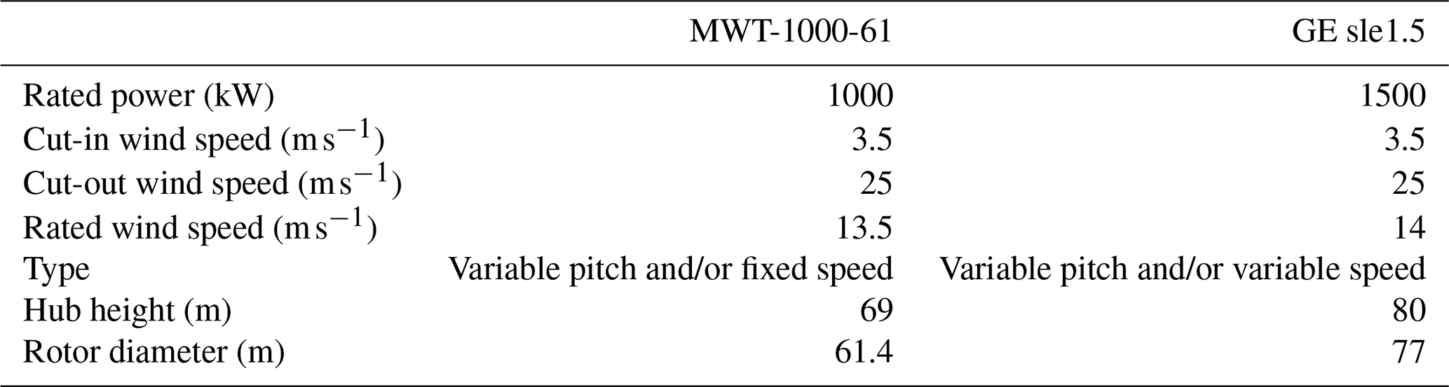
Lidar data collected during an experimental campaign carried out at an onshore wind farm are used to assess the potential of the LiSBOA algorithm for wind energy applications. The measurements were collected during a long-term experimental campaign conducted at a large wind farm located in northeastern Colorado (Fig. 1). This wind park encompasses 221 Mitsubishi 1-MW and 53 General Electric 1.5-MW wind turbines. More technical specifications of the wind turbines are provided in Table 1.

Figure 1 Map of the wind farm under investigation. (a) Top view of the wind farm, with the diameter of the dots representing the turbine rotor diameter (in the wind rose, the sectors where both meteorological (met) towers are potentially affected by turbine wakes are displayed in lighter color). (b) Area probed through StreamLine XR lidar on 11 and 12 October 2018. (c) Typical field of view of the WindCube 200S lidar.

Table 1 Technical specifications of the wind turbines under investigation.

The wind rose, based on 3 years of wind speed and direction measured by the two meteorological (met) towers present on the site, reveals a prevalence of northwesterly and southeasterly wind directions. A characteristic of this site is the presence of a steep escarpment, with an average jump in altitude of about 80 m, surrounding a relatively flat plateau where the turbines are installed.

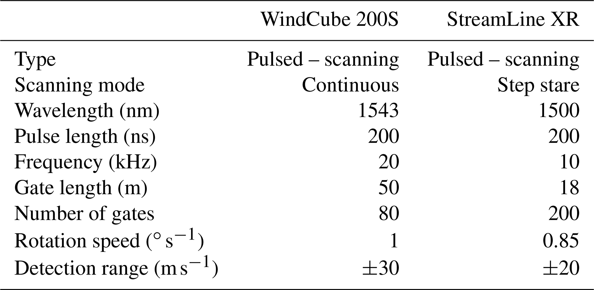
A total of two pulsed Doppler scanning wind lidars were deployed. A WindCube 200S manufactured by Leosphere (Fig. 2a) was installed for the period May–December 2018 in the southern part of the farm, with the scope of detecting turbine wakes and flow distortions induced by the topography. The lidar was connected to the University of Texas at Dallas (UTD) mobile lidar station (El-Asha et al., 2017; Zhan et al., 2019) for remote control, scan setup, and data acquisition. Furthermore, a StreamLine XR by HALO Photonics (Fig. 2b) was deployed for the period 11–19 October 2018 at specific sectors to investigate wake interactions and topography-related flow features. Additional details about the lidars, including the settings adopted for the present study, are provided in Table 2.

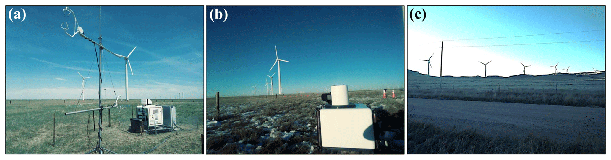
Figure 2 Photographs of the lidar experiment. (a) Lidar WindCube 200S and sonic anemometers (Campbell Scientific, Inc.; CSAT3). (b) Lidar StreamLine XR. (c) GE 1.5sle turbines of the B row.

Table 2 Technical specifications and settings of the wind lidars deployed during the field campaign.

The atmospheric stability is characterized through the Obukhov length (Monin and Obukhov, 1959) retrieved by two CSAT3 3D sonic anemometers manufactured by Campbell Scientific, Inc., which were deployed in the proximity of the UTD mobile lidar station at 1.4 and 2.8 m above the ground. A total of two met towers are installed in the northern part of the park, as shown in Fig. 1. Each tower is equipped with four anemometers installed in a paired configuration at heights of 50 and 80 m, for met tower no. 1, and 50 and 69 m, for met tower no. 2. Mean and standard deviation of wind speed and direction are stored every 10 min, along with the mean temperature and barometric pressure. In the present work, wind velocity data at each height are corrected for the flow distortion due to the tower following the guidelines provided by the International Electrotechnical Commission (IEC) standards (International Electrotechnical Commission 61400-12-1, 2017, Annex G). Additionally, mean and standard deviation over 10 min periods of nacelle wind speed, power, revolutions per minute (RPM), and blade pitch, collected and stored by the supervisory control and data acquisition (SCADA) system, were made available. Normalized average power, P_norm, and C_p curves based on the nacelle anemometers are built by leveraging data for the period 2016–2018 and shown in Fig. 3 as a function of the density-corrected normalized wind speed (International Electrotechnical Commission 61400-12-1, 2017) as follows:

$$\begin{array}{}\text{(1)}& U_{\text{norm}}={\displaystyle \frac{U_{\text{SCADA}}}{U_{\text{rated}}}}\cdot {\left({\displaystyle \frac{{\mathit{\rho }}_{\text{met}}}{{\mathit{\rho }}_{\text{ref}}}}\right)}^{\mathrm{1}/\mathrm{3}},\end{array}$$

where ρ_ref=1.225 kg m⁻³ is the reference density at the sea level, U_SCADA is the 10 min average of the wind speed measured by the nacelle-mounted anemometers, while the local air density ρ_met is calculated from the meteorological data according to the international standard (International Electrotechnical Commission 61400-12-1, 2017). Another important parameter derived from the SCADA data is the turbulence intensity at the rotor, which is defined as follows:

$$\begin{array}{}\text{(2)}& {\text{TI}}_{\text{SCADA}}={\displaystyle \frac{U_{\text{SD, SCADA}}}{U_{\text{SCADA}}}},\end{array}$$

where U_SD, SCADA is the standard deviation of wind speed over 10 min periods.

Figure 3 Performance curves for the General Electric (GE) and Mitsubishi (MHI) wind turbines. (a) Normalized power, P_norm, and (b) power coefficient, C_p.

The two lidars performed a great variety of scans during the campaign, based on the specific phenomena under investigation. For the present analysis, we focus on the 3D reconstruction of noninteracting wakes using the high-resolution data collected with the Halo StreamLine XR lidar and the 2D reconstruction of multiple overlapping wakes detected by the WindCube 200S.

3 Application of LiSBOA to volumetric lidar data

This section aims to explore the potential of LiSBOA for the selection of the optimal azimuthal resolution of a lidar scan, data postprocessing, and reconstruction of 3D flow statistics. The data set used in this section was collected on 11 October 2018 over the farm region, shown in Fig. 1b, through a StreamLine XR lidar. The goal of the experiment is to investigate the evolution of multiple turbine wakes advected over complex terrain. Figure 4 shows the site of the deployment and the relative distances between the lidar and the turbine hubs.

Figure 4 Satellite map of deployment of Halo StreamLine XR on 11 October 11 2018. Source: ©Google Maps.

The deployment location was chosen to scan the wakes generated by wind turbines B16–B19 for south-southeast (SSE) wind directions. The lidar was deployed off a county road that connects the plateau with the surrounding plains, with a consequent difference in altitude between the instrument and the base of the turbines of about 40 m. To probe the wake region of turbines B16–B19 (Fig. 2c) and the leeward side of the ridge, seven PPI scans were performed by sweeping an azimuthal range of 65^∘ with elevations angles, β, set to 5, 6, 7, 8, 10, 12, and 15^∘. The total sampling time was selected equal to T=1 h, since the local weather forecast service provided by the wind farm operator predicted 1 h of steady wind conditions, blowing in a SSE mean direction and having a speed of U_∞≈6 m s⁻¹. The aerosol concentration allowed for the selection of a gate length of Δr=18 m and accumulation time of 1.2 s.

As reported in Sect. 4 of Letizia et al. (2021), several parameters of the flow under investigation are required for the optimal design of the lidar scans. The fundamental half wavelengths typical for wind turbine wakes were selected equal to those used in Sect. 5 of Letizia et al. (2021), i.e., $\mathrm{\Delta }{n}_{\mathrm{0},x}=\mathrm{2.5}D$ and $\mathrm{\Delta }{n}_{\mathrm{0},y}=\mathrm{\Delta }{n}_{\mathrm{0},z}=\mathrm{0.5}D$. Similarly, the integral timescale was chosen equal to $\mathit{\tau }{U}_{\mathrm{\infty }}/D=\mathrm{0.4}$ (τ∼5 s). Finally, a measurement volume with dimensions of 1000, 950, and 130 m in the streamwise, transverse, and vertical directions, respectively, was selected to probe wakes generated from turbines B16–B19 and the downwind region of the escarpment. The expected characteristic velocity standard deviation was estimated to be $\sqrt{\stackrel{\mathrm{‾}}{u^{\prime \mathrm{2}}}}=\mathrm{0.125}{U}_{\mathrm{\infty }}$, based on previous field measurements of turbine wakes under stable conditions (Zhan et al., 2019).

For the selection of the optimal azimuthal angular resolution of the lidar scan, LiSBOA is applied to produce a Pareto front for six possible angular resolutions, Δθ, between 0.25 and 4^∘, and four values of the smoothing parameter, $\mathit{\sigma }=[\mathrm{1}/\mathrm{4},\mathrm{1}/\mathrm{6},\mathrm{1}/\mathrm{8},\mathrm{1}/\mathrm{17}]$. As shown in Fig. 5, the optimal lidar scan is that with angular resolution $\mathrm{\Delta }\mathit{\theta }=\mathrm{1}{}^{\circ }$ and $\mathit{\sigma }=\mathrm{1}/\mathrm{4}$ or $\mathit{\sigma }=\mathrm{1}/\mathrm{6}$. Generally, an increasing Δθ entails a reduction in the standard deviation of the mean, ϵ^II, yet values higher than $\mathrm{\Delta }\mathit{\theta }=\mathrm{1}{}^{\circ }$ do not lead to significant reductions in ϵ^II, while worsening the data loss, ϵ^I, indicating a larger number of grid points not satisfying the Petersen–Middleton constraint.

Figure 5 Pareto front for the design of the optimal lidar scan for the reconstruction of the wakes generated by wind turbines B16–B19. The markers highlighted in red correspond to the respective parameters obtained from the actual lidar data after the quality control process.

In Fig. 5, the values of the cost function ϵ^I and ϵ^II, calculated from the lidar data after the quality control process (Beck and Kühn, 2017), are also reported for the optimal angular spacing of the lidar $\mathrm{\Delta }\mathit{\theta }=\mathrm{1}{}^{\circ }$. It is noteworthy that there is a negligible difference between the values calculated before and after the quality control of the lidar data, indicating that the data loss due to the acquisition error is negligible in the domain of interest. The spatial distributions of the grid points satisfying the Petersen–Middleton constraint for different values of Δθ and $\mathit{\sigma }=\mathrm{1}/\mathrm{4}$ are reported in Fig. 6. It can be observed, as $\mathrm{\Delta }\mathit{\theta }=\mathrm{1}{}^{\circ }$ represents the highest angular step, ensuring an acceptable coverage of the spatial domain.

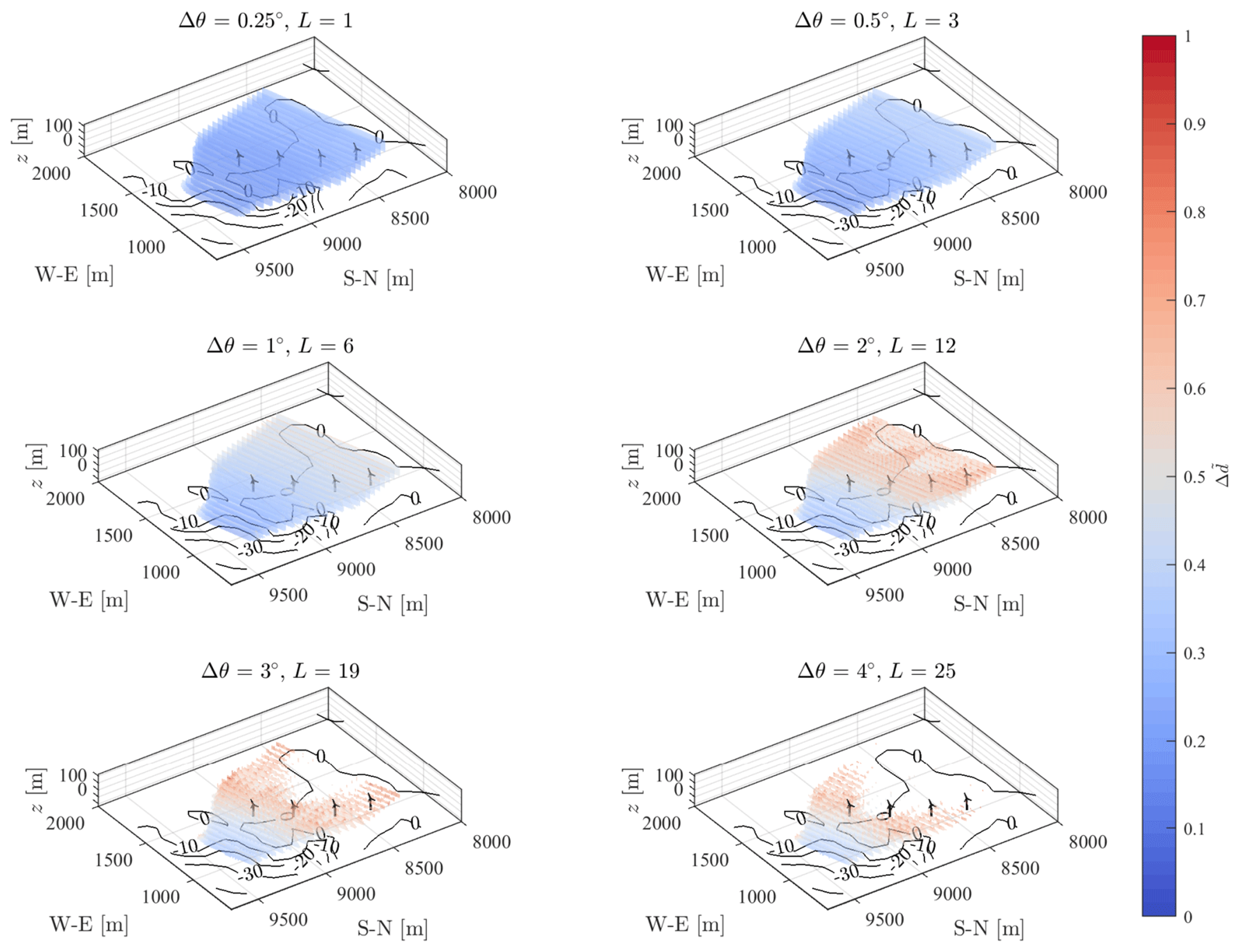
Figure 6 Random data spacing, $\mathrm{\Delta }\stackrel{\mathrm{̃}}{d}$, for six volumetric scans with different angular resolution and $\mathit{\sigma }=\mathrm{1}/\mathrm{4}$. Points violating the Petersen–Middleton constraint ($\mathrm{\Delta }\stackrel{\mathrm{̃}}{d}>\mathrm{1}$) are not displayed.

The data collected, adopting the optimal scanning strategy with $\mathrm{\Delta }\mathit{\theta }=\mathrm{1}{}^{\circ }$, are now postprocessed to calculate the mean streamwise velocity and turbulence intensity. The time series of the wind speed and direction recorded by the sensors installed on met tower no. 1 at hub height and located at a distance of 2700 m in the northern direction of the test site are leveraged to characterize the incoming wind. The evolution of wind speed and direction along with the velocity field, measured with three specific PPI scans, are reported in Fig. 7. For the period between 20:30 and 21:30 local time (Mountain daylight time – MDT), and indicated by the shaded area in Fig. 7a and b, the wind speed remained within the range between 5.1 and 7.1 m s⁻¹, while the wind direction departed less than 10^∘ from its mean value of ${\stackrel{\mathrm{‾}}{\mathit{\theta }}}_{\mathrm{w}}=\mathrm{163.4}{}^{\circ }$. The wind and power data, which are recorded by SCADA (Fig. 8), confirm that the turbines experienced fairly homogeneous inflow conditions, with the differences in power capture being 5 % smaller than the rated value. The values of normalized velocity, together with the performance curves (Fig. 3), indicate that the turbines were operating in region II of the power curve for the whole interval of interest.

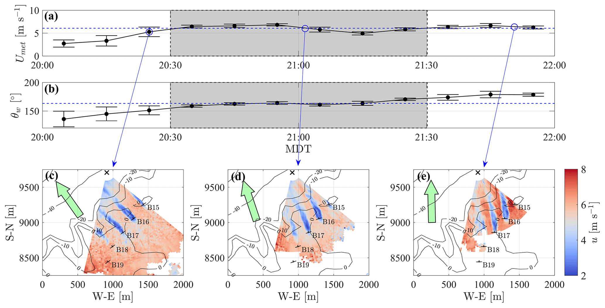
Figure 7 3D lidar scans of five wind turbines. (a) The 10 min average wind speed measured from the anemometers installed at 50 and 80 m height on met tower no. 1. The error bar represents the standard deviation over 10 min. The shaded area represents the interval selected for the LiSBOA application. (b) The 10 min average wind direction in the geophysical reference system measured from the vanes installed at 50 and 80 m on met tower no. 1. (c–e) Equivalent velocity fields measured with PPI scans at different times. The green arrow is oriented as being the mean wind direction measured by met tower no. 1, while the black cross indicates the lidar location.

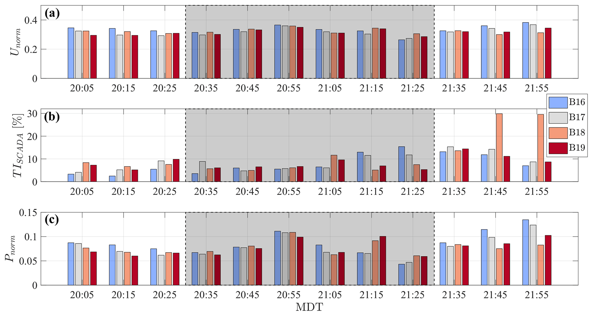
Figure 8 SCADA data during the selected testing period. (a) Normalized hub height velocity. (b) Turbulence intensity. (c) Normalized power.

Since statistical stationarity is an important assumption for the LiSBOA applications, adequate postprocessing of the lidar data is needed to avoid effects on the reconstructed flow statistics due to the wind variability. Specifically, the wind speed variability is corrected by making the line-of-sight velocity nondimensional with the incoming wind speed. To this end, the instantaneous velocity field measured by the lidar is divided by the synchronized mean wind speed obtained from met tower no. 1, as explained above. Furthermore, scans performed when the wind direction was outside of the range $\stackrel{\mathrm{‾}}{{\mathit{\theta }}_{\mathrm{w}}}\pm \mathrm{\Delta }{\mathit{\theta }}_{\mathrm{w}}/\mathrm{2}$, with $\mathrm{\Delta }{\mathit{\theta }}_{\mathrm{w}}=\mathrm{10}{}^{\circ }$, are excluded. After the quality control based on the dynamic filtering (Beck and Kühn, 2017), 169 000 data points out of 455 000 are made available for the LiSBOA reconstruction on a Cartesian grid, with resolution equal to dx=0.25Δn₀. Isolated grid regions violating the Petersen–Middleton constraint (<2 % of the total number of grid points) are rejected, and their respective values are filled through a Laplacian interpolation (inpaint_nans.m in MATLAB). This analysis is restricted to the streamwise component of the wind velocity, which is estimated using the equivalent velocity approach (Zhan et al., 2019). The nondimensional equivalent velocity is referred to as $\stackrel{\mathrm{‾}}{u}/U_{\mathrm{\infty }}$ in the remainder of the paper, while the associated turbulence intensity is referred to as $\sqrt{\stackrel{\mathrm{‾}}{u^{\prime \mathrm{2}}}}/\stackrel{\mathrm{‾}}{u}$.

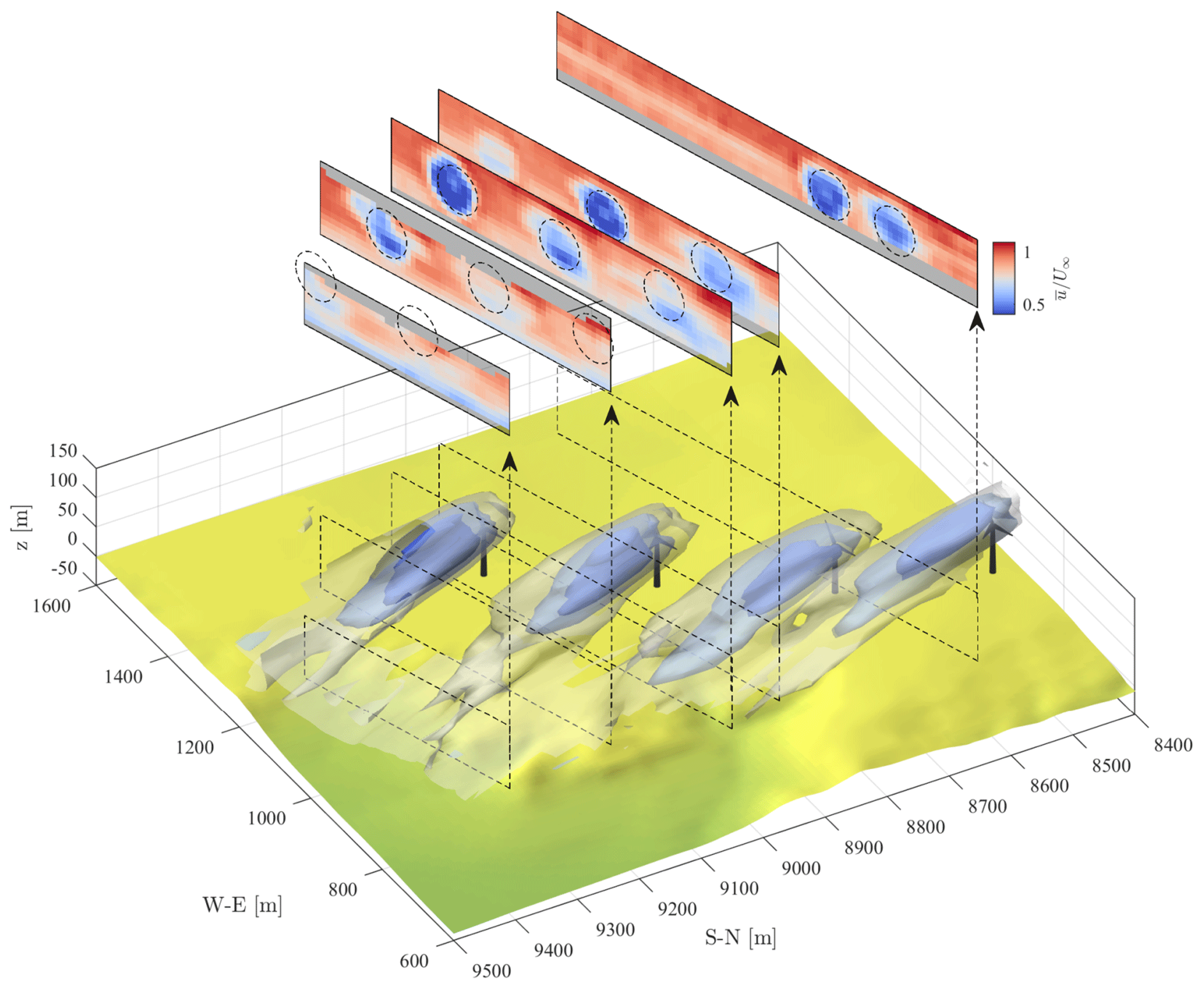
Figure 9 3D rendering of the normalized mean equivalent velocity field reconstructed with $\mathrm{\Delta }{\mathit{\theta }}_{\mathrm{w}}=\mathrm{10}{}^{\circ }$. The three isosurfaces represent $\stackrel{\mathrm{‾}}{u}/U_{\mathrm{\infty }}=\mathrm{0.45}$, 0.6, and 0.75, while the color maps represent cross sections of the mean velocity field over the respective planes reported in the rendering. The dashed circles correspond to the rotor-swept area of turbines B16–B19 (from left to right) projected onto the specific cross-plane.

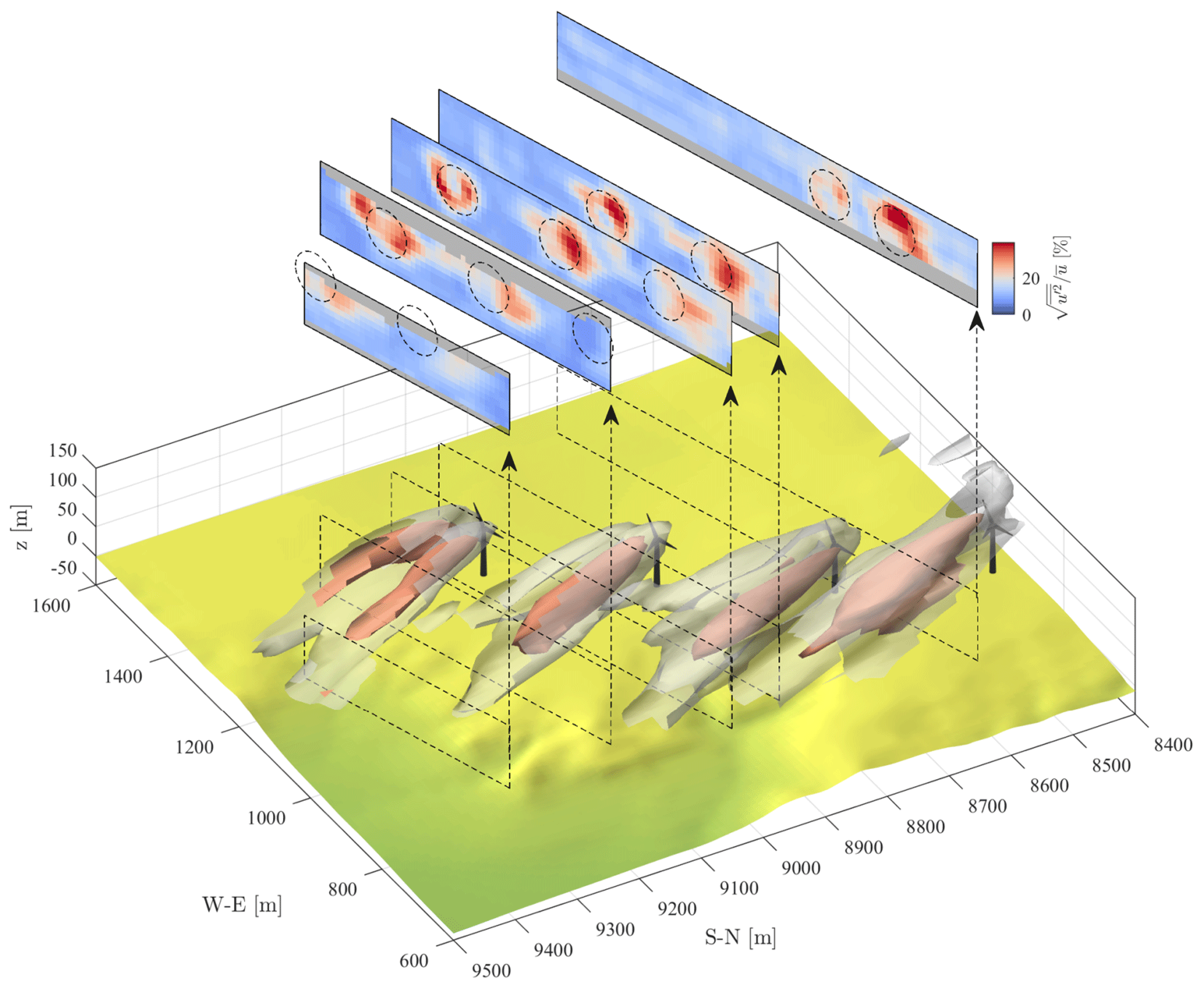
Figure 10 3D rendering of the turbulence intensity field reconstructed with $\mathrm{\Delta }{\mathit{\theta }}_{\mathrm{w}}=\mathrm{10}{}^{\circ }$. The two isosurfaces represent $\sqrt{\stackrel{\mathrm{‾}}{u^{\prime \mathrm{2}}}}/\stackrel{\mathrm{‾}}{u}$ levels of 20 % and 30 %, while the color maps represent cross sections of the turbulence intensity field over the respective planes reported in the rendering. The dashed circles correspond to the rotor-swept area of turbines B16–B19 (from left to right) projected onto the specific cross-plane.

Figures 9 and 10 show 3D renderings of the nondimensional velocity and turbulence intensity fields obtained by using the parameters $\mathit{\sigma }=\mathrm{1}/\mathrm{4}$ – m=5. Wake features, such as turbulent diffusion, the high-momentum jet in the hub region, and the turbulent shear layer at the wake boundary, are well-captured. A total of two highly turbulent regions are located on both sides of the wakes, which is a distinctive signature of wake meandering occurring mostly horizontally in the atmospheric boundary layer (ABL; España et al., 2011). The lack of symmetry and similarity among different turbines, however, suggests that full statistical convergence is not achieved on the second-order statistics for the available data set. The low-speed region hovering over the downslope most probably represents the upper part of the low momentum zone that occurs past sharp escarpments (Berg et al., 2011).

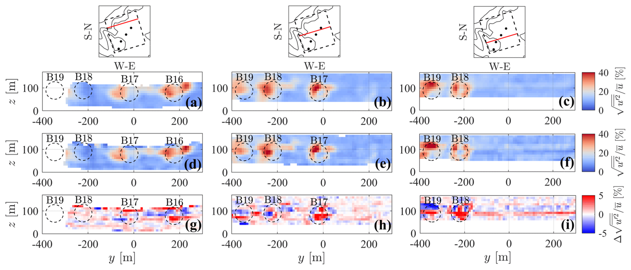
Figure 11 Comparison of the turbulence intensity reconstructed with $\mathit{\sigma }=\mathrm{1}/\mathrm{4}$ – m=5 (a, b, c) vs. $\mathit{\sigma }=\mathrm{1}/\mathrm{6}$ – m=2 (d, e, f) and their difference (g, h, i) for three selected streamwise locations indicated by the red lines in the top maps.

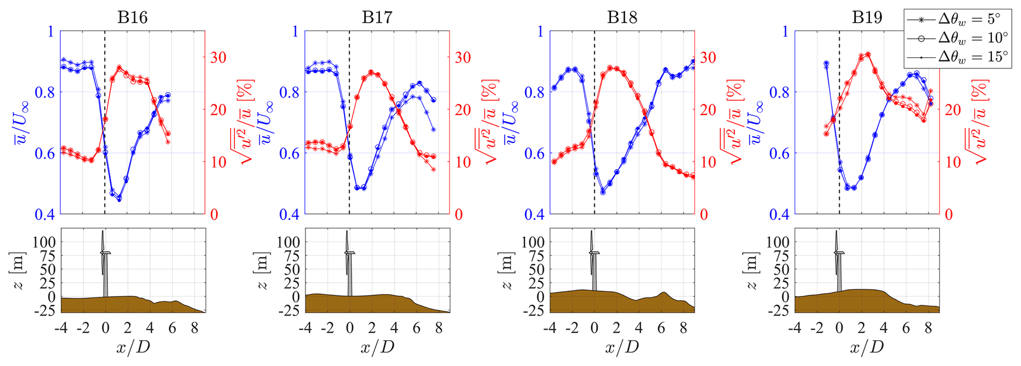
Figure 12 Rotor-averaged streamwise mean velocity and turbulence intensity as a function of the downstream distance from the turbine and associated altitude profile.

The effect of the combination σ – m on higher-order statistics is investigated by extracting the turbulence intensity at different cross-stream planes. The optimal pairs σ−m identified by the Pareto front analysis (Fig. 5), namely $\mathit{\sigma }=\mathrm{1}/\mathrm{4}-m=\mathrm{5}$ and $\mathit{\sigma }=\mathrm{1}/\mathrm{6}-m=\mathrm{2}$, are tested here. One may expect that, due to the difference in the response of the high-order moments of the fundamental mode between the two pairs, $D^{\mathrm{0}}\left(\mathbf{\Delta }{\stackrel{\mathrm{̃}}{\mathit{n}}}_{\mathbf{0}}\right)$, the first case would exhibit a significantly lower $\sqrt{\stackrel{\mathrm{‾}}{u^{\prime \mathrm{2}}}}/\stackrel{\mathrm{‾}}{u}$ with respect to the second one. However, as shown in Fig. 11, the peaks of turbulence intensity are quite similar between the two cases. The main difference between the two reconstruction processes is a smoother distribution of $\sqrt{\stackrel{\mathrm{‾}}{u^{\prime \mathrm{2}}}}/\stackrel{\mathrm{‾}}{u}$ for $\mathit{\sigma }=\mathrm{1}/\mathrm{4}-m=\mathrm{5}$. The similarity between the two cases is due, essentially, to the following two reasons: first, the smallest energy-containing length scales of the turbulence intensity field (i.e., shear layer thickness) are larger than the selected fundamental mode $\mathrm{\Delta }{n}_{\mathrm{0},y}=\mathrm{\Delta }{n}_{\mathrm{0},z}=\mathrm{0.5}D$; second, the larger number of points per grid node averaged for the $\mathit{\sigma }=\mathrm{1}/\mathrm{4}$ case, leads to a higher variance due to the reduction in the bias of the estimator of the variance, which partially compensates the lower theoretical response. In summary, this sensitivity analysis suggests that the choice of the σ−m pair cannot be based purely on the theoretical response, since it does not take into account the nonideal effects deriving from the discrete and nonuniform data distribution. Instead, an a posteriori analysis of the statistics retrieved is recommended to select the best σ−m values.

Turbine-wake statistics are extremely sensitive to the width of the selected wind sector (Barthelmie et al., 2009; Hansen and Barthelmie, 2014). It is well known that widening the wind direction range can lead to an enhanced wake diffusion and turbulence intensity (Trujillo et al., 2011; Kumer et al., 2015), which is compensated by higher data availability and statistical significance. A sensitivity analysis to the wind sector width for reconstructing the statistics through LiSBOA for two additional values of Δθ_w is now presented. Besides the baseline value of 10^∘, the effects of a narrower ($\mathrm{\Delta }{\mathit{\theta }}_{\mathrm{w}}=\mathrm{5}{}^{\circ }$) and wider ($\mathrm{\Delta }{\mathit{\theta }}_{\mathrm{w}}=\mathrm{15}{}^{\circ }$) range are investigated. The standard deviation of the wind direction associated with the different sectors is 1.08, 1.93, and 2.74^∘ for $\mathrm{\Delta }{\mathit{\theta }}_{\mathrm{w}}=\mathrm{5},\mathrm{10},\mathrm{15}{}^{\circ }$, respectively. Figure 12 shows the rotor-averaged velocity and turbulence intensity for each turbine as a function of the downstream distance from the rotor. The profiles of the mean and standard deviation obtained for different Δθ_w are practically the same, indicating that the effects of the wind direction variability on wake flow statistics are not significant.

Figure 13 Fields reconstructed adopting several Δθ_w values and sampled at $x/D\sim \mathrm{1.3}$ downstream of turbines B16, B17, B18, and B19. (a) Mean streamwise velocity and (b) streamwise turbulence intensity.

For the sake of completeness, the velocity and turbulence intensity sampled in the cross-stream plane, where the maximum velocity deficit occurs ($x/D\sim \mathrm{1.3}$), for all the turbines and the Δθ_w are shown in Fig. 13. The discrepancies due to different Δθ_w are negligible. A more evident mismatch can be observed in the shape of the wakes among different wind turbines, with the wake of turbine B19, in particular, showing the velocity deficit and turbulence peak that are displaced above the hub height. Turbine B19 is also the only one facing a slightly inclined terrain (see Fig. 12), which may have caused a skewed inflow.

4 Application of LiSBOA to interacting wind turbine wakes

An assessment of the accuracy of LiSBOA in the calculation of mean wind speed and turbulence intensity is now provided for lidar measurements performed during the occurrence of wake interactions. To this end, point-wise measurements provided by the nacelle-mounted anemometers and saved in the SCADA data of four closely spaced Mitsubishi wind turbines, roughly aligned with the wind direction, are compared with the statistics obtained from the postprocessing of the lidar data with LiSBOA.

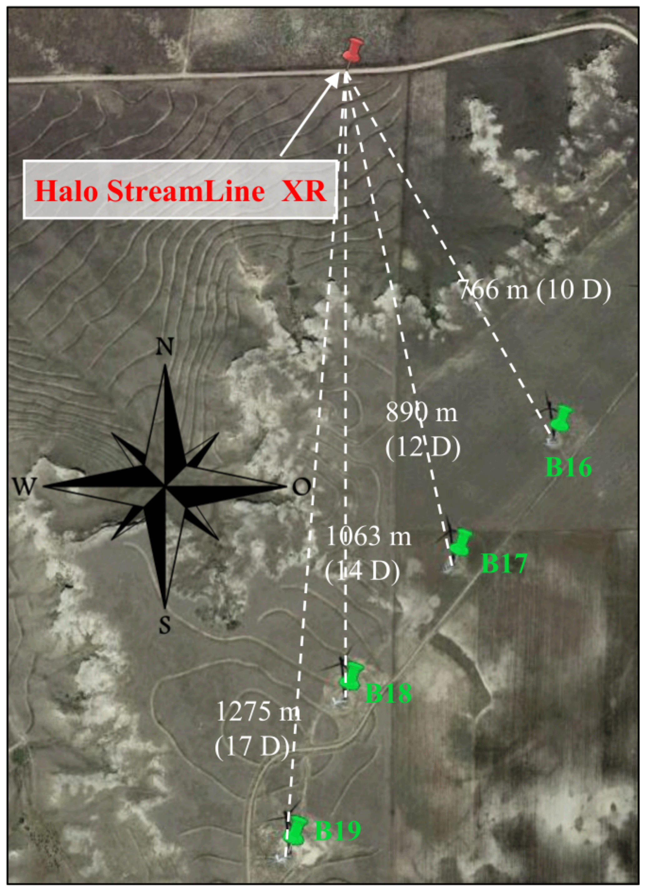
Figure 14 Satellite map of the site for the deployment of the WindCube 200S lidar, including the four Mitsubishi wind turbines under investigation. Source: ©Google Maps.

Figure 14 reports a satellite image of the site used in this experiment. The tests were performed during the occurrence of a nearly steady northeasterly wind (U_∞∼8 m s⁻¹) from 21:00 to 01:00 local time (T=4 h) in the night between 5 and 6 September 2018. This wind condition created a good alignment of the wakes emitted by the turbines F01 to F04. The aerosol conditions allowed us to run the WindCube 200S lidar with a gate length of 50 m and an accumulation time of 0.5 s. The lidar is located at a distance of about 25D from wind turbine F04, which is the most downstream turbine for that specific wind condition, while the average streamwise spacing between the turbines is 3.6D. The velocity and turbulence intensity fields are reconstructed over a horizontal plane, including only points within the vertical range spanning from the bottom-tip to the top-tip of the turbine rotors. The 2D reconstruction adopted here implies that a uniform weight is applied for points displaced at different z, which means the reconstructed statistics represent time-averaged and vertically averaged fields. This 2D approach is deemed convenient for the comparison with point-wise measurements recorded by SCADA through nacelle-mounted instruments as it represents an average of the wind characteristics over the rotor.

The region of interest was probed through a volumetric scan consisting of three PPI scans with elevation angles β=2.1, 2.6, and 3.3^∘. The fundamental half wavelengths were selected as $\mathrm{\Delta }{n}_{\mathrm{0},x}=\mathrm{2.25}D$ and $\mathrm{\Delta }{n}_{\mathrm{0},y}=\mathrm{0.75}D$. According to the previous cases, the integral timescale was estimated to be $\mathit{\tau }{U}_{\mathrm{\infty }}/D=\mathrm{0.4}$ (τ∼3 s). The characteristic velocity standard deviation was set to $\sqrt{\stackrel{\mathrm{‾}}{u^{\prime \mathrm{2}}}}=\mathrm{0.2}{U}_{\mathrm{\infty }}$. The value of the associated turbulence intensity is higher than that used for nonoverlapping wakes to account for the turbulence build-up, which is known to occur for turbines operating experiencing wake interactions (Chamorro and Porté-Agel, 2011; Iungo et al., 2013a).

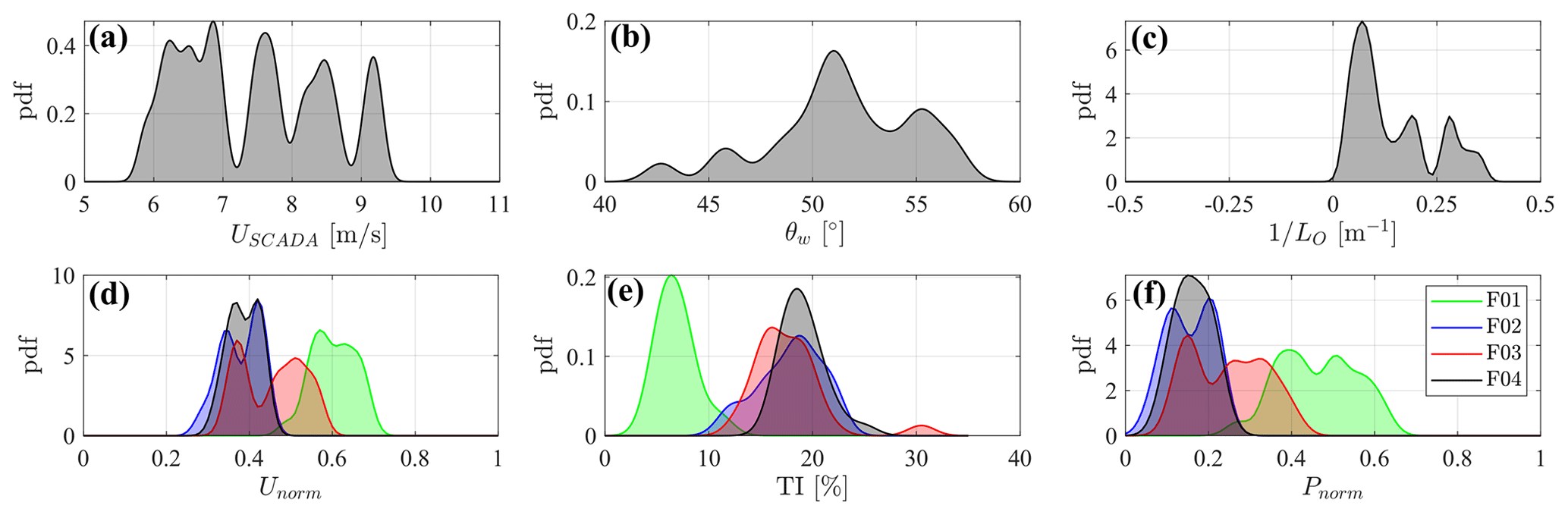
Figure 15 Probability density functions of met and SCADA data recorded from 21:00 to 01:00 MDT in the night between 5 and 6 September 2018. (a) Wind speed from met towers. (b) Wind direction from met towers. (c) Inverse Obukhov length from our sonic anemometers. (d) Normalized wind speed from SCADA. (e) Turbulence intensity from SCADA. (f) Normalized power from SCADA.

The incoming wind is characterized by averaging measurements collected from all the anemometers and wind vanes installed on both met towers, which are located 12 and 10.4 km away from the leading turbine F01 (Fig. 15). The Obukhov length is calculated from both sonic anemometers, indicating a stable stratification regime. The SCADA data exhibit the typical signature of multiple wake interactions with reduced wind speed and power for downstream turbines, while turbulence intensity is enhanced, in particular for the F02 and F04 wind turbines.

Figure 16 Pareto front for the design of the optimal lidar scan for the reconstruction of the wakes statistics for turbines F01–F04. The markers highlighted in red represent the actual lidar data after quality control.

Figure 17 Velocity statistics of the wakes generated by turbines F01–F04 reconstructed over the horizontal plane at hub height. (a) Mean streamwise velocity and (b) streamwise turbulence intensity. The black dots indicate the sampling locations used for the estimation of the incoming flow for the respective turbine.

The optimal design of the lidar scan is performed, considering six values of Δθ and four values of σ. The obtained Pareto front is shown in Fig. 16, which indicates $\mathrm{\Delta }\mathit{\theta }=\mathrm{0.5}{}^{\circ }$ and $\mathit{\sigma }=\mathrm{1}/\mathrm{3},\mathrm{1}/\mathrm{4}$ or $\mathrm{1}/\mathrm{6}$ as the optimal scanning parameters. The equivalent velocity retrieved by the lidar is made nondimensional with the free stream velocity provided by the met towers. The wind direction range is set to Δθ_w=10^∘, resulting in a total measuring period of 150 min. Data points lying above the top-tip or below the bottom-tip heights are excluded for this data analysis. The dynamic filter technique is used to reject corrupted lidar data, producing a total of 544 000 quality controlled lidar samples over 1 327 000 collected lidar data within the selected wind direction range.

LiSBOA is carried out on a grid with resolution dx=0.25Δn₀, using the combination smoothing parameters – number of iterations $\mathit{\sigma }=\mathrm{1}/\mathrm{6}$ – m=1, which is, among the allowable combinations, the one providing the largest response of the higher-order moments. The obtained velocity and turbulence intensity fields over the horizontal plane at hub height are displayed in Fig. 17. The velocity deficit of F02 appears slightly larger than that detected behind the unwaked turbine F01, which is most probably due to the wake superimposition. An even deeper velocity deficit can be observed behind F03, which operates in a partially waked condition for this specific wind direction. Downstream of the third turbine, the wake deficit build-up saturates, confirming results from previous studies on close wake interactions (Barthelmie et al., 2010; Chamorro and Porté-Agel, 2011). Finally, the relatively fast recovery of the wake of the trailing turbine, F04, can be ascribed to the enhanced mixing due to the wake-generated turbulence. Indeed, Fig. 17b shows significant wake-generated turbulence increasing past the leading turbine that reaches its maximum at a distance of 1D downstream of the rotor of F03. Interestingly, wake-generated turbulence is concentrated on the sides of the wake of F01, which experiences undisturbed flow, while it spreads around the whole wake region for the downstream turbines. This feature might be related to the presence of coherent wake vorticity structures in the near wake of turbine F01 (Iungo et al., 2013a; Viola et al., 2014; Ashton et al., 2016), while, further downstream, the perturbed inflow promotes the breakdown of such coherent structures, leading to more homogeneous turbulence. Finally, the large velocity deficit and/or high turbulence detected in the wake of F03 may be a consequence of the mentioned partial wake interaction, which exposes the rotor to a nonhomogeneous flow, resulting in a severely off-design operation.

From a more quantitative standpoint, the incoming wind conditions experienced by each turbine are characterized to perform a direct comparison with the nacelle anemometer data. To this aim, the mean velocity and turbulence intensity profiles are extracted from the lidar statistics at a distance of 1D upstream of the rotors over a segment spanning the whole rotor diameter. The sampling location is chosen based on previous studies (Politis et al., 2012; Hirth et al., 2015), since 1D is generally considered the minimum distance upstream of the rotor where the influence of the induction zone can be neglected for normal operative conditions. The averaged values of $\stackrel{\mathrm{‾}}{u}/U_{\mathrm{\infty }}$ and $\sqrt{\stackrel{\mathrm{‾}}{u^{\prime \mathrm{2}}}}/\stackrel{\mathrm{‾}}{u}$ of each upstream profile are then used for the comparison with the respective values recorded through SCADA.

A well-posed comparison of the wind statistics obtained from LiSBOA, SCADA, and met data requires two important elements. First, the statistical moments compared have to be equivalent; second, both the LiSBOA and SCADA data must be representative of the free stream conditions experienced by each turbine.

Regarding the first issue, the mean field obtained through LiSBOA, $\stackrel{\mathrm{‾}}{u}$, can be expressed as follows:

$$\begin{array}{}\text{(3)}& {〈{\displaystyle \frac{u}{U_{\mathrm{\infty }}}}〉}_T={〈{〈{\displaystyle \frac{u}{U_{\mathrm{\infty }}}}〉}_{\widehat{T}}〉}_T\sim {〈{\displaystyle \frac{U_{\text{SCADA}}}{U_{\text{met}}}}〉}_T,\end{array}$$

where 〈.〉_T is the average calculated over the whole sampling period of 150 min, while $\langle .{\rangle }_{\widehat{T}}$ is the 10 min average performed by SCADA and the met tower acquisition system. U_SCADA and U_met are the 10 min averaged velocities recorded from SCADA and the met tower, respectively, while the symbol ∼ indicates statistical equivalence.

Similarly, for the comparison between the velocity variance calculated through LiSBOA and the respective values recorded through SCADA, we have the following relationship:

$$\begin{array}{}\text{(4)}& {\displaystyle }\begin{array}{rl}{〈{\displaystyle \frac{u^{\prime \mathrm{2}}}{U_{\mathrm{\infty }}^{\mathrm{2}}}}〉}_T& ={〈{〈{\displaystyle \frac{{\widehat{u}}^{\prime \mathrm{2}}}{U_{\mathrm{\infty }}^{\mathrm{2}}}}〉}_{\widehat{T}}〉}_T+{〈{〈{\displaystyle \frac{u}{U_{\mathrm{\infty }}}}〉}_{\widehat{T}}^{\mathrm{2}}〉}_T-{〈{〈{\displaystyle \frac{u}{U_{\mathrm{\infty }}}}〉}_{\widehat{T}}〉}_T^{\mathrm{2}}\\ & \sim {〈{\displaystyle \frac{U_{\text{SD, SCADA}}^{\mathrm{2}}}{U_{\text{met}}^{\mathrm{2}}}}〉}_T+{〈{\displaystyle \frac{U_{\text{SCADA}}^{\mathrm{2}}}{U_{\text{met}}^{\mathrm{2}}}}〉}_T\\ & -{〈{\displaystyle \frac{U_{\text{SCADA}}}{U_{\text{met}}}}〉}_T^{\mathrm{2}},\end{array}\end{array}$$

where u^′ and ${\widehat{u}}^{\prime }$ are the velocity fluctuations with zero mean calculated over the period T and $\widehat{T}$, respectively. The parameter $U_{\text{SD, SCADA}}^{\mathrm{2}}$ is the velocity variance recorded by SCADA over the period $\widehat{T}$ of 10 min.

Figure 18 Met tower and turbines selected for the nacelle transfer function estimation. The directions highlighted in gray represent the valid wind sectors unaffected by turbine wake interactions. The dashed circles bound the allowed range of distances from the tower in compliance with IEC standard 61400-12-1 (International Electrotechnical Commission 61400-12-1, 2017).

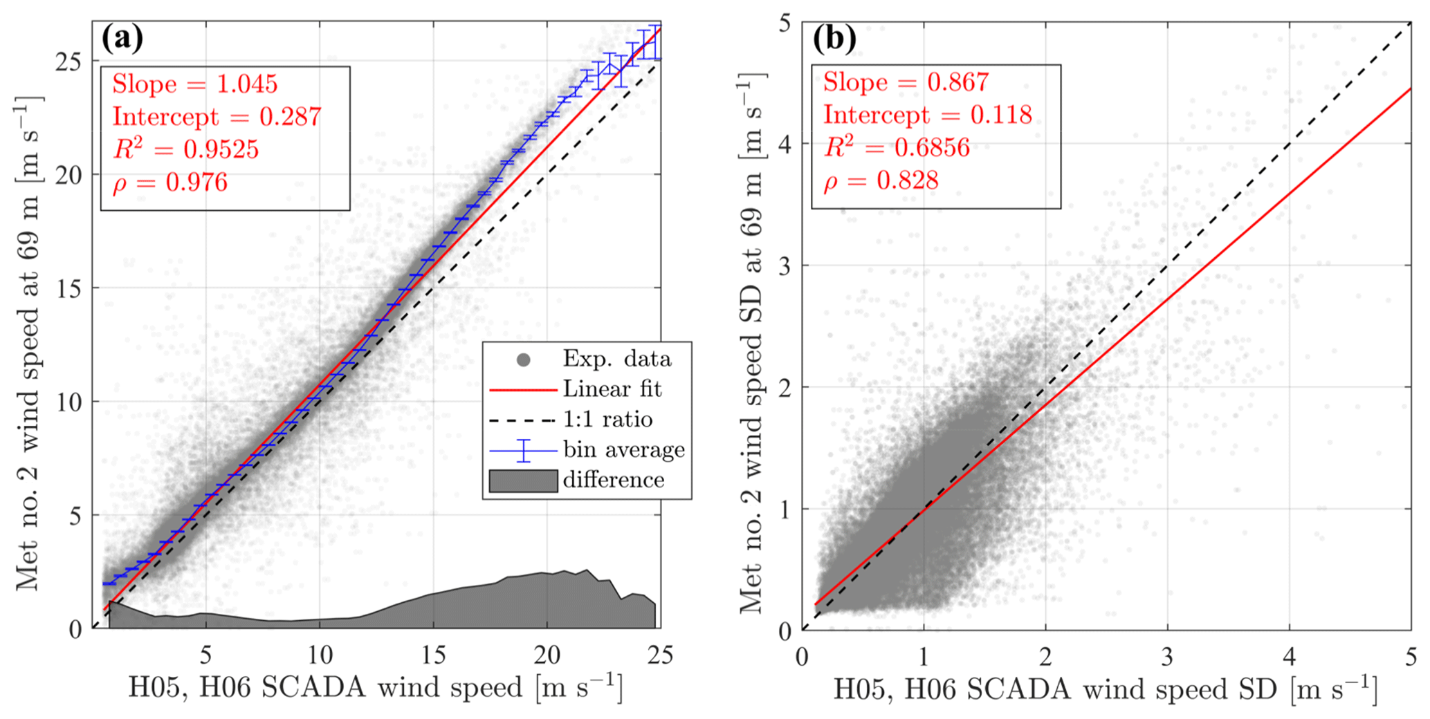
Figure 19 Nacelle transfer function for mean (a) and standard deviation (b) of wind speed. The error bars represent the standard error on the mean with 95 % confidence level.

To ensure that the SCADA mean and standard deviation of velocity are representative of the undisturbed wind conditions at each rotor, these velocity statistics are corrected for the flow distortion induced by the turbine through appropriate nacelle transfer functions (NTFs), which convert the velocity statistics measured at the nacelle of a wind turbine to the corresponding free stream values measured from a met tower located nearby. The IEC standard 61400-12-2 (International Electrotechnical Commission, 61400-12-2) prescribes the calculations of the NTF from the bin average, with bin size 0.5 m s⁻¹, of the velocity measured by a reference anemometer as a function of the nacelle wind speed. In the present work, besides correcting the mean wind speed as indicated by the IEC standards, a linear correction of the wind speed standard deviation is also applied, as suggested by Argyle et al. (2018). We adopted, as reference, an anemometer that is installed at 69 m above the ground on met tower no. 2. The SCADA data of Mitsubishi turbines H05 and H06, both falling in the range of distances from the met tower recommended by the IEC 61400-12-1 (International Electrotechnical Commission 61400-12-1, 2017), are used. Only the unwaked wind sectors calculated based on the same standard are considered. The described layout is shown in Fig. 18, while Fig. 19 shows the result of this analysis. There is a high correlation between the velocity measured by the met tower and the nacelle-mounted anemometer (ρ=0.976). Nevertheless, the NTF of the velocity reveals consistently lower values occurring at the nacelle compared to the met tower, with a peak at 20 m s⁻¹. Concerning the standard deviation of velocity, the agreement between the SCADA and met tower data is significantly lower (ρ=0.828), yet a linear correction can be still calculated with acceptable significance (error on slope and intercept are 0.0038 and 0.0034, with 95 % confidence).

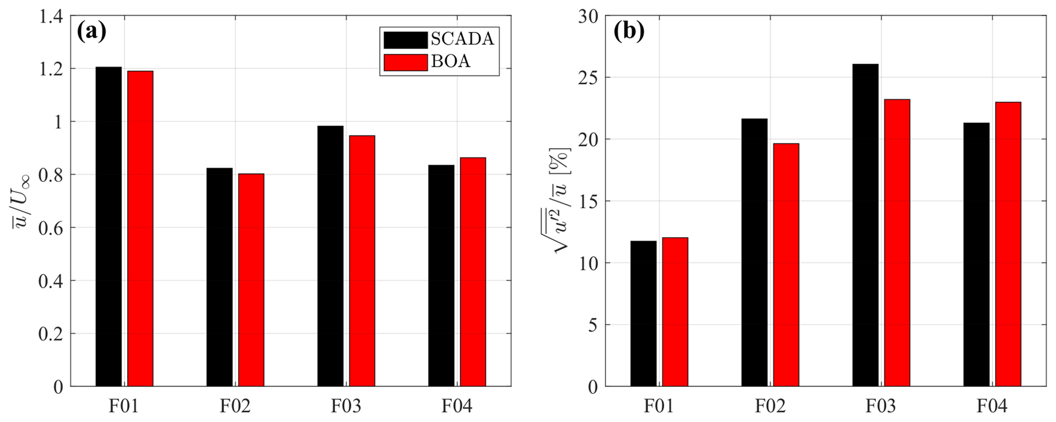
Figure 20 Comparison between LiSBOA and SCADA wind statistics for a case with wake interactions. (a) Mean streamwise velocity normalized by free stream velocity. (b) Streamwise turbulence intensity.

The results of the comparison between LiSBOA and SCADA are provided in Fig. 20. The mean velocity is accurately captured and confirms that F02 and F04 are the turbines mainly affected by the upstream wakes. The slightly higher momentum impinging F03 is mostly due to the imperfect alignment of that rotor with the upstream turbine wakes, which creates a condition of partial wake interaction. A slightly larger discrepancy between LiSBOA and SCADA data is observed for the turbulence intensity, with a maximum difference of ∼3 % for F03. Nonetheless, the main trend is well reproduced, and the overall agreement is satisfactory. The observed difference in turbulence intensity can be related to several factors, such as turbulence damping due to the lidar-measuring process and LiSBOA calculations, the accuracy of the NTF, the estimate of the streamwise velocity from the lidar radial velocity, or the vertical dispersive stresses.

The effect of the sampling location upstream of the turbines in the LiSBOA field is investigated by quantifying the discrepancy of the LiSBOA statistics with respect to the reference SCADA values for all the turbines through the 95th percentile of the absolute error, AE₉₅. Figure 21 shows AE₉₅ as a function of the distance upstream, where the incoming flow is extracted from the LiSBOA statistics. For the mean velocity, it is confirmed that the value suggested by the literature ($x=-\mathrm{1}D$) is sufficiently far from the rotor to limit the effects of the induction zone on the definition of the reference free stream velocity. Furthermore, the rotor thrust does not seem to have noticeable effects on the incoming turbulence, in that the induction zone is essentially devoid of significant turbulent fluctuations due to the loads of the turbine blades. The discrepancy between the turbulence intensity retrieved through LiSBOA and SCADA steeply increases for sampling locations further than 2D from the rotor.

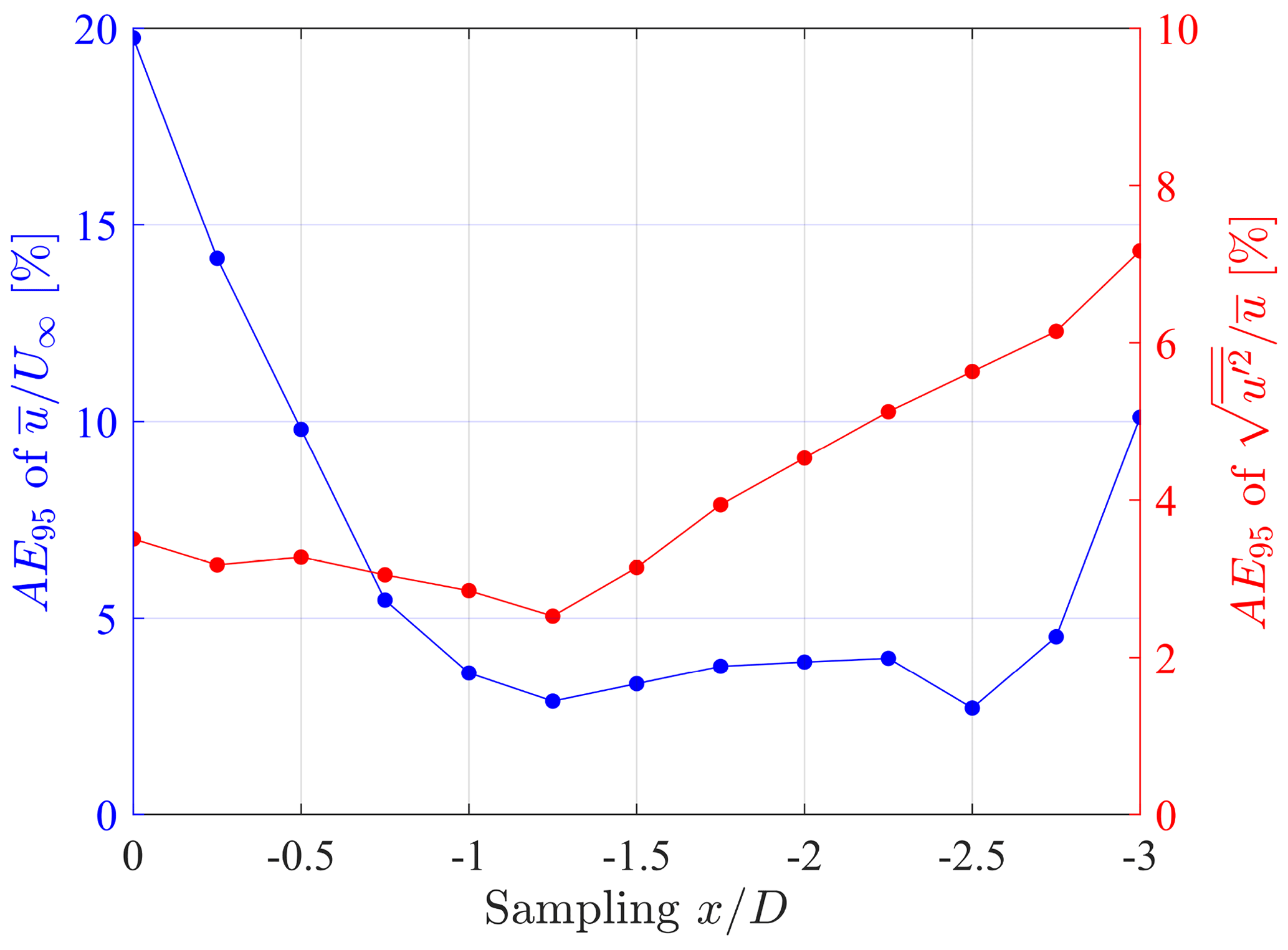
Figure 21 AE₉₅ of mean velocity and turbulence intensity for F01–F04 as a function of the upstream sampling location of the LiSBOA fields.

In summary, the satisfactory agreement between LiSBOA and SCADA data achieved in the present study indicates the proposed procedure as a promising candidate for wind resource assessment, especially for complex terrains, and investigations of the intra-wind-farm flow.

5 Conclusions

The LiDAR Statistical Barnes Objective Analysis (LiSBOA) has been applied to two different cases of wind turbine wakes to estimate the optimal azimuthal step of the lidar and retrieve mean velocity and turbulence intensity fields.

First, LiSBOA has been used to process real lidar data collected for a utility-scale wind farm. For the first test case, the statistics of the wakes of four noninteracting 1.5 MW turbines placed at the brink of an escarpment have been reconstructed. The optimal azimuthal resolution of the lidar scan has been selected through LiSBOA, while the mean velocity and turbulence intensity fields retrieved through LiSBOA have offered a detailed insight of the wake morphology. Furthermore, a sensitivity analysis of the wind direction range has confirmed the robustness of the data selection and quality control methods.

Subsequently, the complex velocity field arising from the interaction of four 1 MW turbines has been analyzed by calculating first- and second-order moments on the horizontal plane. The mean velocity and turbulence intensity extracted 1D upstream of the rotors have agreed well with the values provided by the nacelle anemometers, with maximum discrepancies as low as 3 % of the undisturbed wind speed for the mean velocity and 3 % (in absolute terms) for the turbulence intensity.

The applications of LiSBOA discussed in this work aim to showcase the potential of the proposed procedure for the optimal design of lidar scans and to provide guidelines for the utilization of LiSBOA for the analysis of lidar data. A total of two noticeable advantages of LiSBOA arise from the present work. First, once the wavelengths of interest and the lidar basic scanning parameters dictated by the atmospheric conditions and target position are selected, LiSBOA allows a systematic and effective optimization of the azimuthal resolution, which includes all the essential information of the flow under investigation and the lidars used. This feature can be of interest, especially when planning field experiments that involve multiple lidars, complex topography, or articulated turbine configurations. In such situations, the use of the proposed quantitative and comprehensive scan design approach may be beneficial for narrowing down a great deal of arbitrariness and uncertainty associated with campaign planning. Second, LiSBOA offers complete control over the response of the spatial wavelengths of the velocity field for the statistical moments with various orders. This feature is crucial when dealing with turbulent and multiscale flows because it allows the extraction of meaningful information from the flow while filtering out small-scale variability.

Appendix A: List of symbols

x, y, z	Streamwise, spanwise, and vertical
	Cartesian coordinates
t	Time
ρ	Air density
u, v, w	Streamwise, spanwise, and vertical
	velocity components
L	Number of realizations and/or scans
θ	Azimuth angle
β	Elevation angle
Δθ	Azimuth angle resolution
τa	Accumulation time
Δr	Gate length
Nr	Number of range gates along the laser per beam
T	Total sampling time
σ	Smoothing parameter
m	Number of iterations
Rmax	Radius of influence
Δn	Half-wavelength vector
Δn0	Fundamental half-wavelength vector
Δd	Random data spacing
dx	Resolution vector in Cartesian coordinates
Dm	Response at the mth iteration
ϵI	Cost function I (data loss)
ϵII	Cost function II (standard deviation of
	the sample mean)
τ	Integral timescale
$\stackrel{\mathrm{̃}}{.}$	Spatial variable in the scaled frame of reference
D	Rotor diameter
Unorm	10 min averaged normalized density-corrected
	hub height wind speed
Pnorm	10 min averaged normalized active power
U∞	10 min averaged undisturbed incoming wind speed
USCADA	10 min averaged hub height wind speed
USD, SCADA	10 min based hub height standard deviation
	of wind speed
TISCADA	10 min based hub height turbulence intensity
Umet	10 min averaged wind speed from met tower
LO	Obukhov length