Retrieval of stratospheric aerosol size distribution parameters using satellite solar occultation measurements at three wavelengths

In this work, a novel approach for the determination of the particle size distribution (PSD) parameters of stratospheric sulfate aerosols is presented. For this, ratios of extinction coefficients obtained from SAGE III/ISS (Stratospheric Aerosol and Gas Experiment III on the International Space Station) solar occultation measurements at 449, 756 and 1544 nm were used to retrieve the mode width and median radius of a size distribution assumed to be monomodal lognormal. The estimated errors at the peak of the stratospheric aerosol layer, on average, lie between 20 % and 25 % for the median radius and 5 % and 7 % for the mode width. The results are consistent in magnitude with other retrieval results from the literature, but a robust comparison is difficult, mainly because of differences in temporal and spatial coverage. Other quantities like number density and effective radius were also calculated. A major advantage of the described method over other retrieval techniques is that both the median radius and the mode width can be retrieved simultaneously, without having to assume one of them. This is possible due to the broad wavelength spectrum covered by the SAGE III/ISS measurements. Also, the presented method – being based on the analysis of three wavelengths – allows unique solutions for the retrieval of PSD parameters for almost all of the observed extinction spectra, which is not the case when using only two spectral channels. In addition, the extinction coefficients from SAGE III/ISS solar occultation measurements, on which the retrieval is based, are calculated without a priori assumptions about the PSD. For those reasons, the data produced with the presented retrieval technique may be a valuable contribution for a better understanding of the variability of stratospheric aerosol size distributions, e.g. after volcanic eruptions. While this study focuses on describing the retrieval method, and a future study will discuss the PSD parameter data set produced in depth, some exemplary results for background conditions in June 2017 are shown.

1 Introduction

The existence of a permanent aerosol layer in the stratosphere, typically known as the Junge layer, has been known about since the late 1950s when Christian Junge performed balloon-borne in situ measurements there (Junge et al., 1961). The layer resides roughly between 15 and 30 km in the lower stratosphere directly above the tropopause. The aerosols are usually assumed to be droplets of a solution of sulfuric acid and water with a weight percentage of sulfuric acid of around 75 % (Rosen, 1971; Arnold et al., 1998), although small but still relatively uncertain contributions of other compounds such as carbonaceous and meteoric material are possible (Murphy et al., 2007).

Anthropogenic SO₂ emissions play a role in the variation of the stratospheric aerosol (SA) budget (Sheng et al., 2014), but they are dwarfed by natural sources, especially by direct injections due to large volcanic eruptions. Intense biomass burning events, such as the Canadian wildfires in 2017 (Ansmann et al., 2018) and the Australian bushfires of 2019–2020 (Ohneiser et al., 2020), can also play an important role in the feeding of the aerosol layer. Nevertheless, the Junge layer is persistent globally over time, even in volcanically quiescent periods and without large biomass burning events (Kremser et al., 2016). The stratospheric aerosol layer is then mainly sustained by a flux of sulfurous aerosols and precursor gases from the troposphere, such as SO₂ and OCS (Sheng et al., 2014), which are eventually oxidized to H₂SO₄, which itself forms new H₂SO₄–H₂O-droplets by co-condensation with water vapour (Hamill et al., 1990). The formed aerosols grow through coagulation and further condensation, while sedimentation limits the averaged aerosol size in the aerosol layer. In the stratosphere, evaporation, due to rising temperatures with height, generally determines the upper boundary of the aerosol layer. The most important region for this transport of sulfur-bearing substances from the troposphere to the stratosphere is the tropical tropopause layer (TTL) (Kremser et al., 2016).

Stratospheric aerosols play a role in the chemistry of Earth's atmosphere and its radiative balance. Regarding the former, they influence the levels of different atmospheric constituents, like NO_x (Deshler, 2008) and stratospheric ozone, when SA levels are elevated due to volcanic eruptions (Hofmann and Solomon, 1989; Gleason et al., 1993). Additionally, they can act as condensation nuclei for the formation of polar stratospheric clouds (PSCs), which are central in catalytic ozone destruction during polar winter and spring (Deshler, 2008).

Concerning the radiative balance of the atmosphere, SA absorb and emit longwave radiation, thereby having a warming effect on the stratosphere, and contribute to the extinction of solar radiation mainly by scattering, thus leading to a cooling of the troposphere (Dutton and Christy, 1992). All of those effects are critically dependent on the size distribution of the aerosols, with smaller particles at a constant aerosol mass being more efficient at destroying ozone (Robock, 2015) and larger particles being more efficient at scattering solar radiation, which leads to the aforementioned cooling of the troposphere. However, the cooling effect is dominant only up to a certain size (effective radius of about 2 µm), above which their absorptive capacity surpasses their scattering capacity, and they have a net warming effect on Earth's surface (Lacis et al., 1992).

The great importance of the size of stratospheric aerosols is the reason Robock (2015) stated that the question about changing aerosol size after large SO₂ injections into the stratosphere is one of the most outstanding research questions regarding the link between volcanic eruptions and the associated climate response.

Mathematically, the size distributions of SA are usually expressed as lognormal functions (see Eq. 1), based on fits to the longest available set of in situ measurements carried out from Laramie, Wyoming (Deshler et al., 2003). A monomodal lognormal distribution is expressed as follows:

$$\begin{array}{}\text{(1)}& {\displaystyle \frac{\mathrm{d}N\left(r\right)}{\mathrm{d}r}}={\displaystyle \frac{N_{\mathrm{0}}}{\sqrt{\mathrm{2}\mathit{\pi }}\cdot r\cdot \ln \mathit{\sigma }}}\cdot \exp \left(-{\displaystyle \frac{{\ln }^{\mathrm{2}}\left(r/r_{\mathrm{med}}\right)}{\mathrm{2}{\ln }^{\mathrm{2}}\mathit{\sigma }}}\right),\end{array}$$

where r_med is the median radius, σ the mode width of the lognormal distribution and N₀ the total number density. The scattering and absorption cross sections, and thereby the extinction cross section of SA, can be calculated using Mie theory as a function of their composition and the particle size distribution (PSD) parameters (Mie, 1908). Therefore, those parameters can, in principle, be retrieved from extinction coefficients calculated from measurements at multiple wavelengths, with the particle composition in this case being a secondary factor, since the realistic range of the real refractive indices of H₂SO₄–H₂O aerosol droplets is not very large. As a source of these extinction coefficients, satellite data are particularly valuable as, depending on the orbit parameters, a near-global coverage is possible.

The aim of this work is to retrieve the stratospheric aerosol size distribution parameters from the extinction measurements of the SAGE III (Stratospheric Aerosol and Gas Experiment III) instrument mounted on the International Space Station (ISS; Cisewski et al., 2014). Here we assume the lognormal size distribution to be monomodal, which is a common assumption. Please note that we do not claim that the actual stratospheric aerosol size distribution is well described by a monomodal lognormal distribution under all circumstances. While Deshler et al. (2003) regularly fit a bimodal lognormal distribution to their in situ measurements, the existence of a second mode is still controversial, with a gamma distribution also being discussed (Wang et al., 1989; Nyaku et al., 2020). Also, due to the limited degrees of freedom, retrieving the parameters of a bimodal lognormal distribution with the retrieval technique presented in the current work would not be possible. While there are studies in which both the median radius and the mode width of a monomodal lognormal PSD have been retrieved (Wang et al., 1989; Bingen et al., 2003; Wurl et al., 2010; Malinina et al., 2018), with other data sets in the past it was often necessary to fix either the median radius or the mode width to determine the other (Yue and Deepak, 1983; Bourassa et al., 2008; Zalach et al., 2020), or it was only possible to retrieve a range of plausible mode width values (Bauman et al., 2003). In this work, both parameters are retrieved simultaneously, which is possible because of the broad wavelength spectrum of the SAGE III/ISS instrument and the retrieval method described in this study. This method was used successfully in the past to retrieve the PSDs of noctilucent cloud (NLC) particles or polar mesospheric cloud (PMC) particles (von Cossart et al., 1999; Baumgarten et al., 2006).

This work is part of the cooperative research project called VolImpact (Revisiting the volcanic impact on atmosphere and climate – preparations for the next big volcanic eruption), which focuses on the response of the climate system to volcanic eruptions (von Savigny et al., 2020). In particular, it is part of the project VolARC (Constraining the effects of Volcanic Aerosol on Radiative forcing and stratospheric Composition). One of the foci of this project is to better understand the temporal variability of the PSD of stratospheric aerosols.

The main purpose of the present study is to introduce the PSD retrieval approach applied. A full analysis and discussion of all the results obtained from the SAGE III/ISS (Stratospheric Aerosol and Gas Experiment III on the International Space Station) solar occultation measurements will be the topic of a future publication. After shortly introducing the data set used in Sect. 2, we will present the method with which the size distribution parameters were retrieved in Sect. 3 and explain the error calculations made in Sect. 4. Afterwards, latitudinal contour plots and sample vertical profiles of the most important parameters are shown and discussed in Sect. 5, with conclusions in Sect. 6.

2 SAGE III/ISS instrument

The satellite data set that was used in this work to retrieve the PSD parameters comes from the SAGE III instrument that is mounted on the International Space Station since 2017 and is a part of NASA's Earth Observing System (EOS). The instrument is the successor of the satellite experiments SAM II, SAGE I, SAGE II and SAGE III Meteor-3M and performs lunar and solar occultation measurements, measuring the attenuation of solar radiation due to scattering and absorption by atmospheric constituents such as ozone, water vapour and aerosols. On board the ISS, it observes around 15 sunrise and 15 sunset events in 24 h, respectively. While occultation measurements are characterized by a limited spatial and temporal coverage, an important advantage, as opposed to limb scatter measurements, is that atmospheric extinction can be obtained directly, without a priori knowledge of the PSD and phase function. The SAGE III/ISS level 2 solar aerosol product used (version 5.1) contains aerosol extinction coefficients from tangent heights 0 to 45 km, with a grid step size of 0.5 km and a maximum latitudinal range roughly between 69^∘ N and 67^∘ S. The latitude of the sunrise and sunset measurements oscillates with a period of about 2 months, which can be seen in Fig. 1, where the geographic latitude of each event is plotted as a function of time for the available data from 7 June 2017 up until 30 April 2019 (NASA, 2020).

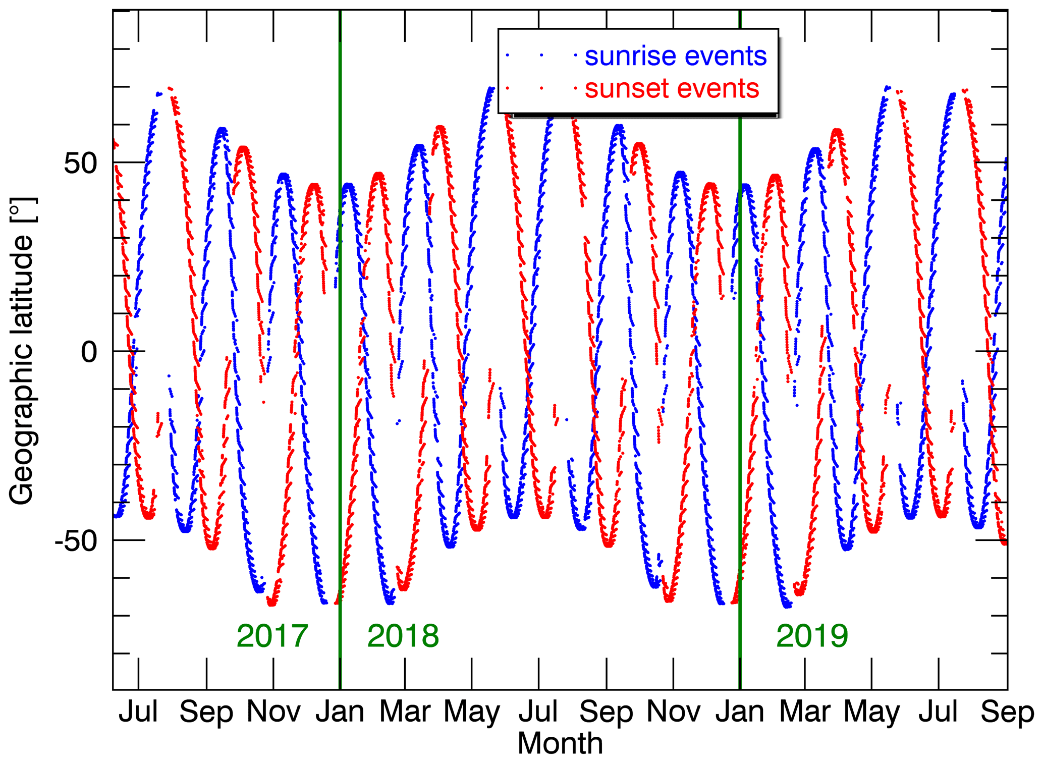
Figure 1 Latitudinal coverage of SAGE III/ISS solar occultation measurements between June 2017 and September 2019. Observed sunrise and sunset events are shown in blue and red, respectively. Green vertical lines mark turns of the year.

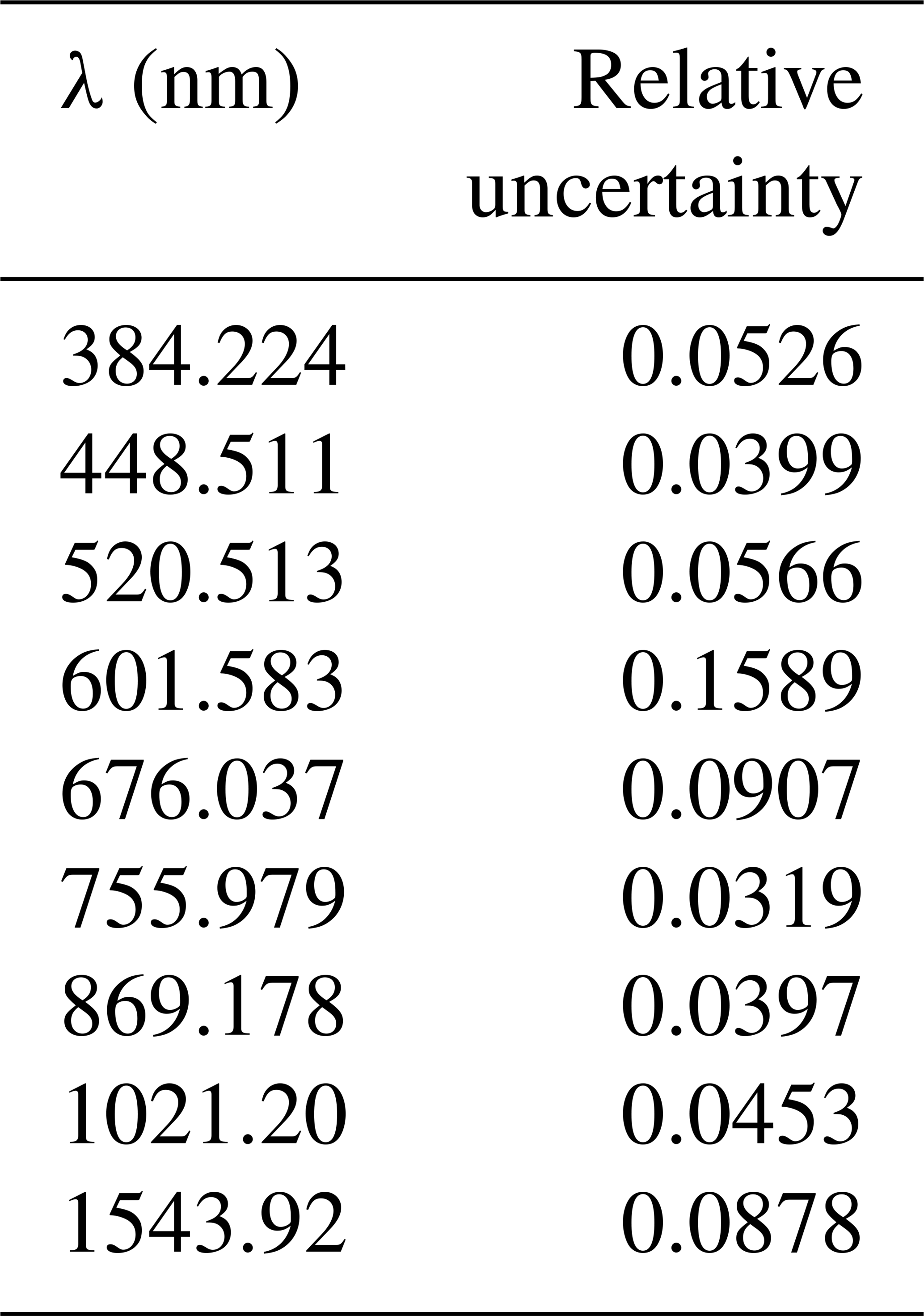
The aerosol extinction coefficients are available at nine wavelengths, shown in Table 1. The 809 pixel charge-coupled device (CCD) array used for the first eight channels measures solar radiance with 1 to 2 nm spectral resolution between 280 and 1040 nm, while the 1543.92 nm channel data are based on measurements with an indium gallium arsenide (InGaAs) infrared photodiode at 1550 nm with a 30 nm bandwidth. Also, the relative uncertainties of the extinction measurements of each channel, averaged between June of 2017 and April of 2019 for the altitude of 20 km, are shown in Table 1. In particular, the 1543.92 nm near-infrared channel significantly extends the spectral range of extinction measurements when compared to SAGE II, the predecessor of this instrument, improving the precision of the method used in this work and rendering a simultaneous retrieval of both the median radius and mode width possible, as will be shown here.

Table 1 Spectral channels of the SAGE III/ISS level 2 solar aerosol product and the respective extinction measurement uncertainties, as provided by the NASA Atmospheric Science Data Center (NASA, 2020), averaged from June 2017 to December 2019 at 20 km altitude.

3 Methodology

In this work, a method similar to the one that von Cossart et al. (1999) used to retrieve the size distribution parameters of noctilucent cloud (NLC) particles from lidar measurements was implemented to derive the median radius and mode width of the stratospheric aerosol size distributions from the SAGE III/ISS aerosol extinction coefficients. For this, at each measured tangent height of a sunrise or sunset event, two ratios of extinction coefficients at three wavelengths from SAGE III/ISS were compared to extinction ratios calculated with a Mie code, provided by Oxford University's Department of Physics (Oxford University, 2018), with predefined PSD parameters at the same wavelengths. These Mie calculations form the basis of the set of curves shown in the left panel of Fig. 2 (discussed below), which is the main tool used for the retrieval and functions as a lookup table.

Figure 2 Extinction ratios at three wavelengths as a result of Mie calculations for values of median radii between 1 and 1000 nm and mode widths between 1.05 and 2.0. The dots mark r_med values with increments of 10 nm. The respective r_med values of five selected dots are shown in the colour corresponding to their mode width. Panel (a) shows the set of curves to be compared to SAGE III/ISS measurements for the PSD parameter retrieval. Panel (b) shows an unusable set of curves with broad areas of non-unique solutions for the PSD parameters due to the closeness of the wavelengths used.

A number of assumptions were made for the Mie calculations and for the retrieval method to be applicable. Sensitivity testing of the retrieval to some of these parameters is discussed in Sect. 4.

• The particles are assumed to consist of a solution of 75 % H₂SO₄ and 25 % H₂O by weight, without other components such as meteoric or carbonaceous material. As a result of this composition, and due to being liquid droplets in the sub-micron size range, the particles can also be assumed to be spherical. Because of this, Mie theory can be applied. This composition also determines the wavelength-dependent real part of the refractive index n that is used in Mie calculations.

• The imaginary part of the refractive index k, or the absorption index, is set to zero since absorption for SA is very low for visible and near-infrared radiation (Palmer and Williams, 1975).

• A monomodal lognormal particle size distribution is used (see Eq. 1). Therefore, the retrieval of r_med, σ and N is the main objective of this paper.

• The physically reasonable range for the mode width of a SA size distribution is assumed to be 1.05 to 2.0 (see discussion below).

Figure 2 shows two sets of curves resulting from the Mie calculations at three wavelengths each. The left panel depicts the set of curves used for the PSD parameter retrieval in this work, and the right panel shows an example with a bad choice of wavelengths, as will be discussed further below. Each coloured curve in both panels consists of the extinction ratios calculated for one constant mode width and median radii between 1 and 1000 nm, in 1 nm increments. The dots on each curve are 10 nm apart for visual clarity.

To obtain a theoretical total aerosol extinction coefficient k_ext for a monomodal lognormal size distribution at a specific wavelength λ, median radius r_med and mode width σ, single aerosol extinction coefficient values calculated with the Mie code (Oxford University, 2018) are integrated over the radius range covered by the particle size distribution (PSD), as shown in Eq. (2). For these Mie calculations of the aerosol extinction coefficient, the median radius and mode width of the size distribution, the total number density N₀ and the real and imaginary refractive index n and k, which are determined by the assumptions made above, have to be assumed. For the calculation of extinction ratios, which are formed from these extinction coefficients and used for the actual size retrieval, the assumption about the number density is irrelevant since the extinction ratios become independent of N₀. The equation for the extinction coefficient is as follows:

$$\begin{array}{}\text{(2)}& k_{\mathrm{ext}}\left(\mathit{\lambda }\right)=\underset{\mathrm{0}}{\overset{\mathrm{\infty }}{\int }}{Q}_{\mathrm{ext}}(r,n,k,\mathit{\lambda })\cdot \mathit{\pi }{r}^{\mathrm{2}}\cdot \mathrm{PSD}\left(r,r_{\mathrm{med}},\mathit{\sigma },N_{\mathrm{0}}\right)\mathrm{d}r.\end{array}$$

Here, Q_ext is the extinction efficiency of the single aerosol, and πr² is the cross-sectional area of the spherical particle. Together, both quantities form the extinction cross section of the single aerosol particle.

In Fig. 3, the dependence of the extinction efficiency of a single H₂SO₄–H₂O aerosol droplet on radius and wavelength is depicted for a radius range of 1 to 1000 nm and the wavelengths 449, 756 and 1544 nm, which are used in the PSD parameter retrieval of the current work. Since absorption is assumed to be zero, the extinction efficiency here is equal to the scattering efficiency. The spectral differences in the extinction efficiencies, depending on the sizes of the aerosol in the size distribution, are the basis for the retrieval of the unknown parameters of that distribution.

Figure 3 Extinction efficiencies of single (monodisperse) aerosols at radii between 1 and 1000 nm from Mie calculations for the three wavelengths used in the retrieval of the current work.

The values for the wavelength-dependent real refractive indices used in the Mie calculations of the lookup table extinction coefficients are based on the measurements performed by Palmer and Williams (1975) at 300 K. Lorentz–Lorenz corrections, as described by Steele and Hamill (1981), were conducted to obtain values at 215 K, which is typical for lower stratospheric temperatures. The temperature-dependent density values of the H₂O-H₂SO₄ solution needed for the corrections were extrapolated from values from Timmermans (1960).

With the lookup table ready, aerosol extinction coefficients from the SAGE III/ISS data set at the same three wavelengths are used to form extinction ratios, which can then be plotted into the 2-D space of the lookup table. This is shown in Fig. 4, where the same set of curves is shown. Each dot with error bars represents a measurement of the same sunset event on 23 June 2017 at 5.2^∘ S and 179.6^∘ W at a different tangent height. Measurements which do not fall within the space of the set of curves (around 4.7 % of measurements at 20 km), which is the case for noisy data, are not shown. For the particular occultation event shown in Fig. 4, the points represent measurements between 18.5 and 32 km. A total of four different grey tones indicate from which 5 km tangent height interval the measurements corresponding to a point originate. The lightest grey, for example, includes the measurements between 15 and 19.5 km, while the darkest (black) points correspond to measurements between 30 and 34.5 km.

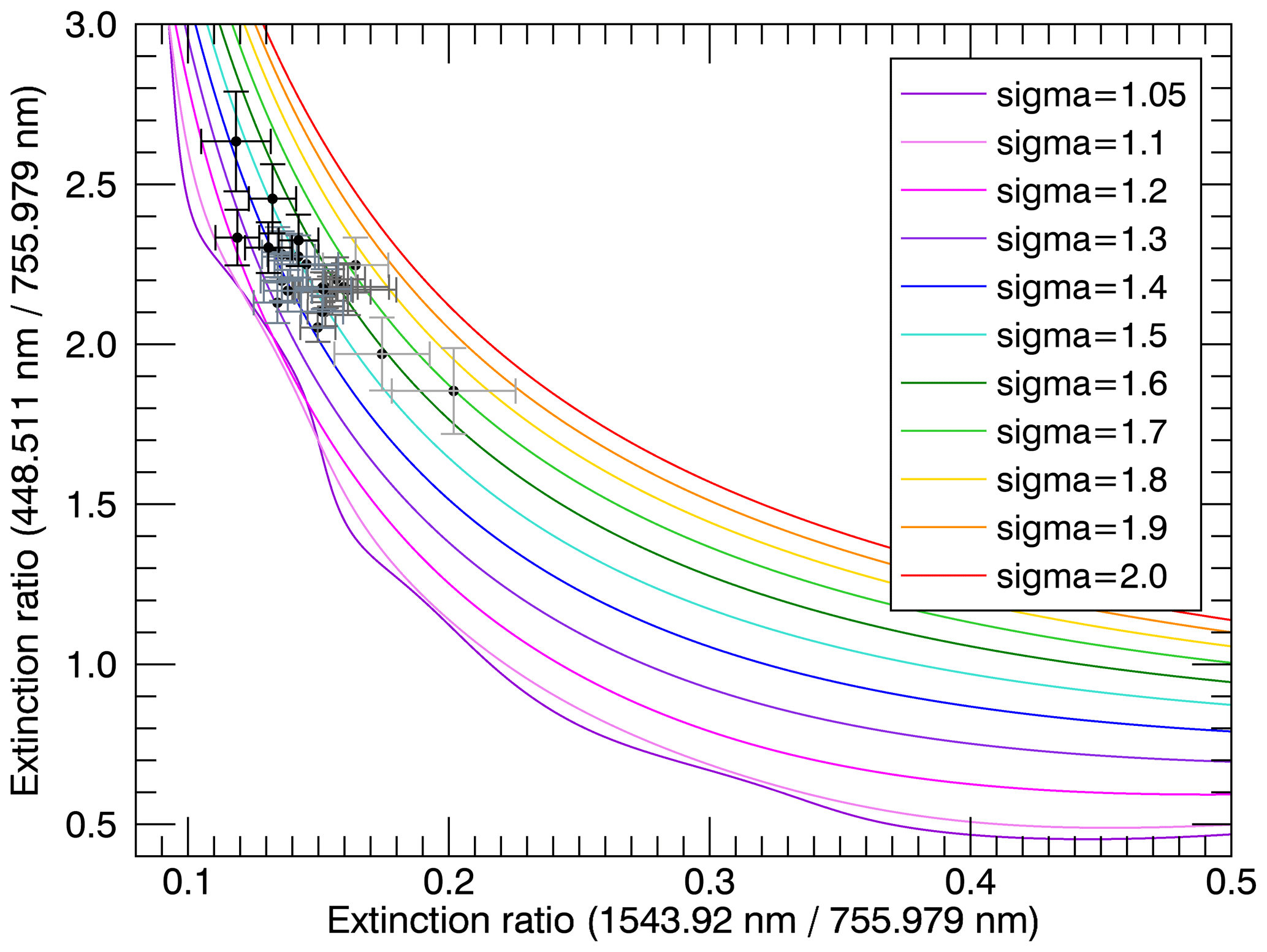
Figure 4 Extinction ratios derived from SAGE III/ISS measurements from one exemplary sunset event at 5.2^∘ S and 179.6^∘ W on 23 June 2017 plotted in the field of the same Mie calculations shown in Fig. 2a, including error bars. Each point represents measurements at a different tangent height. The darker the points and error bars depicted, the higher the corresponding tangent height of the measurement.

Afterwards, r_med and σ can be derived for each tangent height by interpolating between the known values of two points of the Mie calculations above and below on the surrounding curves of the lookup table. This interpolation is done at the extinction ratio coordinates of the measurement data point within the 2-D space of the lookup table; i.e. the error bars play no role in the retrieval itself, only in the identification and exclusion of noisy data later and in the choice of the wavelength combination, as will be discussed next.

The choice of the combination of the three wavelengths used for the retrieval is important because the dependence of the extinction ratio on particle size is strongly dependent on λ, which in turn determines the shape of the calculated curves. For some wavelength combinations, this leads to large areas in the 2-D space of extinction ratios where sets of extinction ratios have multiple solutions for median radius and mode width (see Fig. 2b), while also leading to larger uncertainties in the results that can be retrieved. This is especially the case in λ combinations that span only a small wavelength range, like 384.224/448.511/520.513 nm. In addition, the uncertainties of the extinction measurements performed by SAGE III/ISS also depend on the wavelength channel used, as can be seen in Table 1, in part due to differing contributions of Rayleigh scattering and sensitivity to aerosol. For the retrieval of this work, the λ combination 448.511/755.979/1543.92 nm (Fig. 2a) was chosen because it utilizes most of the wavelength range the SAGE III instrument offers, while avoiding potential problems with a systematic bias in the extinction coefficients in the 384.224 nm channel in the upper troposphere lower stratosphere (UTLS) region because of large contributions of molecular scattering there. Also, the averaged relative measurement uncertainty in the chosen spectral channels is as low as possible, and the 601.583 and 676.037 nm channels, which have the highest uncertainties, are avoided. Although it has higher average relative extinction coefficient uncertainties, the 1543.92 nm channel is used instead of the one at 1021.2 nm. This is because the accuracy with which the median radius and mode width of the aerosol size distribution can be determined in the retrieval does not only depend on the uncertainty of the extinction ratios, i.e. their error bars, but also on how far the individual curves of the lookup table are apart (see Fig. 4). Utilizing a much broader wavelength interval with the use of the 1543.92 nm channel increases this distance between the individual curves of the lookup table, overcompensating the higher extinction ratio uncertainties. We define an accuracy parameter below that can be used to illustrate this, as it takes both factors into account and is used to assess the reliability of the r_med and σ values retrieved. This accuracy parameter a for the retrieved PSD parameters at a specific tangent height is calculated as follows:

$$\begin{array}{}\text{(3)}& a={\displaystyle \frac{{\mathrm{\Delta }}_x}{{\mathit{\delta }}_{f_x}}}\cdot {\displaystyle \frac{{\mathrm{\Delta }}_y}{{\mathit{\delta }}_{f_y}}}.\end{array}$$

Here, Δ_x and Δ_y are the distances between the curves of the Mie calculations with the lowest and highest σ in the direction of one axis, respectively, while ${\mathit{\delta }}_{f_x}$ and ${\mathit{\delta }}_{f_y}$ are the associated propagated measurement uncertainties of the extinction ratios. Therefore, small measurement uncertainties of the extinction coefficients at the three wavelengths coupled with the curves of the Mie calculations being far apart lead to high accuracy parameters, indicating reliable retrieval results.

In Fig. 5, two profiles of the accuracy parameter a averaged over the first 3000 solar occultation events observed by SAGE III/ISS are shown. The red curve is the profile using the wavelength combination 449/756/1544 nm, which is used in the retrieval of the PSD parameters, while the blue curve was calculated using the 1021.2 nm channel instead of the 1543.92 nm channel. The plot clearly shows higher accuracy parameter values, using the 1543.92 nm channel across all altitudes for the reasons discussed above, making this channel much better suited for the retrieval method presented here.

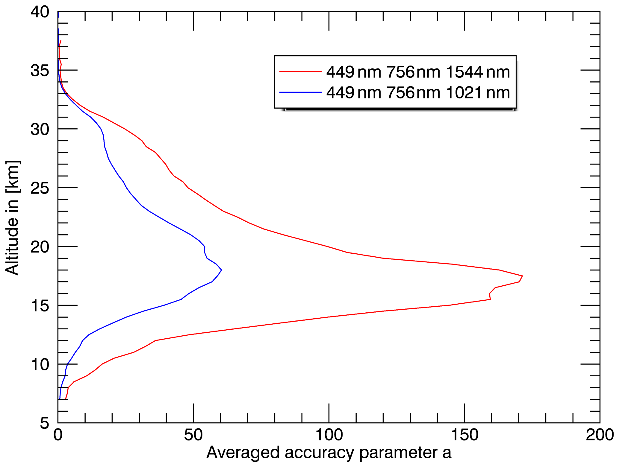
Figure 5 Profiles of the accuracy parameter a averaged over the first 3000 solar occultation events of SAGE III/ISS for the wavelength combination 449/756/1544 nm (red) and 449/756/1021 nm (blue).

The assumption about the physically reasonable range of the mode width of SA is necessary, since with σ values larger than 2.0, the corresponding curves would partly overlap with the previously calculated ones in some areas of the 2-D field of the lookup table, meaning that some retrievals with particularly high mode width would have at least two possible solutions. However, to limit the solutions to a maximum σ of 2.0 is reasonable, firstly, because the associated r_med for higher values would become very small (around 10 nm and smaller). Secondly, these higher mode width values are very rarely found in other retrieval works, for example, Bingen et al. (2004) and Nyaku et al. (2020) do not find values exceeding 1.9. In the in situ measurements by Deshler et al. (2003), where a monomodal lognormal size distribution was found as being the best fit, 7.6 % of the mode width values exceed 2.3 and only 2.97 % exceed 2.5 (data not shown). For the SAGE III/ISS data set analysed so far, only very few measurements fall into the space where overlap exists, if, for example, 2.5 was deemed the maximum realistic value. If, for example, 2.3 was set as the maximum, even fewer values would be affected and so on.

In an effort to minimize the influence of clouds on the retrieval, all measurements below a tangent height of 25 km, at which both the extinction coefficient of the 1021 nm channel is higher than 10⁻⁴ km and the extinction ratio between 449 and 1021 nm is lower than 2, suggesting large particles, are excluded from the analysis. This is a rough filter and may exclude some non-cloud data, but it will generally improve the overall quality of the remaining data.

Once r_med and σ were determined, the aerosol number density N can easily be calculated from the measured extinction coefficient at a single wavelength using the following relation:

$$\begin{array}{}\text{(4)}& N={\displaystyle \frac{k_{\mathrm{ext}}\left(\mathit{\lambda }\right)}{{\mathit{\sigma }}_{\mathrm{ext}}\left(\mathit{\lambda }\right)}},\end{array}$$

with σ_ext(λ), the extinction cross section at one of the three wavelengths used for the retrieval, coming from the just-retrieved r_med and σ, and k_ext(λ) being one of the three extinction coefficients from the SAGE III/ISS data set. In the retrieval data set produced, the wavelength channel at 756 nm was used for these number density calculations since, on average, it has the lowest extinction coefficient uncertainties. However, the average difference between the results with this wavelength choice and one of the other two is below 1 %.

Another useful quantity is the effective radius r_eff, i.e. the area-weighted mean radius (Grainger, 2017). For a lognormal PSD, it can be calculated using the following relation:

$$\begin{array}{}\text{(5)}& r_{\mathrm{eff}}=r_{\mathrm{med}}\cdot \exp \left({\displaystyle \frac{\mathrm{5}}{\mathrm{2}}}\cdot {\ln }^{\mathrm{2}}\left(\mathit{\sigma }\right)\right).\end{array}$$

Moreover, two quantities that can be calculated from the retrieved median radii and mode widths are the mode radius r_mod, defined as follows:

$$\begin{array}{}\text{(6)}& r_{\mathrm{mod}}=\exp \left(\ln \left(r_{\mathrm{med}}\right)-{\ln }^{\mathrm{2}}\left(\mathit{\sigma }\right)\right),\end{array}$$

and ω, a measure of the absolute width of the monomodal lognormal size distribution as introduced by Malinina et al. (2018), which is calculated as follows:

$$\begin{array}{}\text{(7)}& \mathit{\omega }=r_{\mathrm{med}}^{\mathrm{2}}\cdot \exp \left({\ln }^{\mathrm{2}}\left(\mathit{\sigma }\right)\right)\cdot \left(\exp \left({\ln }^{\mathrm{2}}\left(\mathit{\sigma }\right)\right)-\mathrm{1}\right).\end{array}$$

Both quantities are useful because they facilitate a more intuitive understanding of changes in the monomodal lognormal size distribution. The mode radius gives the position of the peak of the distribution in linear space. The problem with the mode width σ is that it is defined relative to the median radius, which means that, on its own, it does not provide much information on the shape of the size distribution. This is where ω is useful since, as the standard deviation of the size distribution, it is given in absolute units and can therefore be interpreted more easily.

4 Error estimation

In order to provide error estimates for the retrieved aerosol size distribution parameters, the sensitivity of the median radius and mode width to the identified main error sources is tested. Those are the quantities that are the necessary input for the Mie calculations forming the basis of the retrieval method used here, namely the imaginary and real parts of the refractive indices of the H₂SO₄–H₂O-droplets and the extinction coefficients, which are available in the SAGE III/ISS solar occultation data set. For each of these quantities, a separate retrieval with perturbed values is performed to obtain error estimates. The total errors resulting from that are shown and discussed in Sect. 5.

While in the regular retrieval the imaginary part of the refractive index k is treated as being zero for each of the three wavelengths used, for the sensitivity testing, values found by Palmer and Williams (1975) are used. While no value was provided for the 449 nm channel, the retrieval here is conducted with k values of 7.6992 × 10⁻⁸ for 756 nm and 1.419 × 10⁻⁴ for the 1544 nm channel attained through interpolation of values given in their paper. Since those are still small values, no large effect is to be expected.

In the Mie calculations, for each used wavelength, a different but fixed value of the real part of the refractive index n is used. Under the assumption of pure sulfate particles, variations in stratospheric temperature and their effect on n are considered for the calculation of errors, since temperature changes will influence the water vapour pressure in the droplet, changing the composition of the aerosol, when equilibrium is re-established (Steele and Hamill, 1981). Based on the temperature profile data in the SAGE III/ISS level 2 solar occultation data, the atmospheric temperature between 10 and 30 km altitude, where the aerosol layer is located, and in the time frame from the start of measurements (June 2017) to December 2019 nearly always stayed within ±30 K of the 215 K value used in the retrieval. For the sensitivity analysis, the real refractive indices are perturbed according to Lorentz–Lorenz corrections of the originally used values from 215 to 245 K. This results in a reduction in n between 0.5 % and 0.6 %, depending on the wavelength. A new retrieval is conducted in this way to determine error estimates for the retrieved PSD parameters.

To investigate the effect of the uncertainties of the extinction coefficient values, which are provided in the SAGE III/ISS data set, those uncertainties are first propagated to obtain the errors of the extinction ratios calculated from the instruments' extinction coefficients. The consequential error bars, which are visualized in Fig. 4, can be seen as forming the major and minor axis of an error ellipse around the point, which is used for the regular retrieval. A size distribution parameter retrieval is performed for eight characteristic points on the error ellipse, and the mean value of the resulting median radius and mode width anomalies is used as the error estimate. Errors using the maximum anomaly obtained in this way are also calculated. They are larger, but not discussed here, since they likely overestimate the actual uncertainties of the retrieved values. There is a portion of the used measurements, for which not all of the eight characteristic points on the error ellipse lie within the confines of the calculated set of curves seen in Fig. 4, which calls the validity of the respective mean error into question. At 20 km altitude, roughly 14 % of the measurements are affected by this. This is why, in plots that show total errors of the median radius or mode width, like Figs. 8 and 7, these values are excluded in order to not falsify the errors shown.

The total error Δ is then calculated in the following way, where δ₁, δ₂ and δ₃ are the individual errors resulting from perturbed imaginary and real parts of the refractive indices and propagated extinction coefficient uncertainties, that were just discussed:

$$\begin{array}{}\text{(8)}& \mathrm{\Delta }=\sqrt{{\mathit{\delta }}_{\mathrm{1}}^{\mathrm{2}}+{\mathit{\delta }}_{\mathrm{2}}^{\mathrm{2}}+{\mathit{\delta }}_{\mathrm{3}}^{\mathrm{2}}}.\end{array}$$

To further validate the retrieval method, Ångström exponents calculated with SAGE III/ISS aerosol extinction coefficients at 449 and 756 nm were compared with Ångström exponents calculated with extinction coefficients obtained from Mie calculations using the retrieved median radii and mode widths. Both results are supposed to be reasonably close to each other. The Ångström exponent is defined as follows:

$$\begin{array}{}\text{(9)}& \mathit{\alpha }=-{\displaystyle \frac{\ln \left(\frac{k_{\mathrm{ext},\mathrm{449}}}{k_{\mathrm{ext},\mathrm{756}}}\right)}{\ln \left(\frac{{\mathit{\lambda }}_{\mathrm{449}}}{{\mathit{\lambda }}_{\mathrm{756}}}\right)}},\end{array}$$

with k_ext being the extinction coefficient at a specific wavelength and λ being that wavelength.

5 Results and discussion

At the time of writing, the SAGE III/ISS solar occultation measurements are ongoing. Starting in June 2017, up to around 900 vertical profiles of extinction coefficients for each spectral channel are available per month, from which profiles of the median radius r_med and mode width σ have been retrieved with the method presented above. Subsequently, the same number of profiles of the mode radius r_mod, absolute mode width ω, number density N and effective radius have also been calculated.

All values below 25 km that fall under both criteria of the cloud filtering explained in Sect. 3 are excluded. For the whole data set used from June 2017 to December 2019, this is 1.37 % of the retrieved data in general but only 0.05 % of the retrieved data in 20 km altitude. Of the remaining data, all values with an associated accuracy parameter a (see Sect. 3) below 16 are excluded, ensuring that particularly noisy data points are filtered out. This removes 8.74 % of the remaining data in general but only 0.88 % of the data in 20 km altitude.

Figure 6 shows contour plots of averaged vertical profiles from 7 to 30 June 2017 for each of the six quantities listed above. In addition, the extinction coefficient at 449 nm, which is provided directly in the SAGE III/ISS solar occultation data set (NASA, 2020), and the extinction ratio at 449 and 756 nm is shown. The contour plots consist of temporal averages of individual profiles sorted in latitude bins of 5^∘. The red line marks the altitude of the tropopause layer as it is provided in the SAGE III/ISS solar occultation data set.

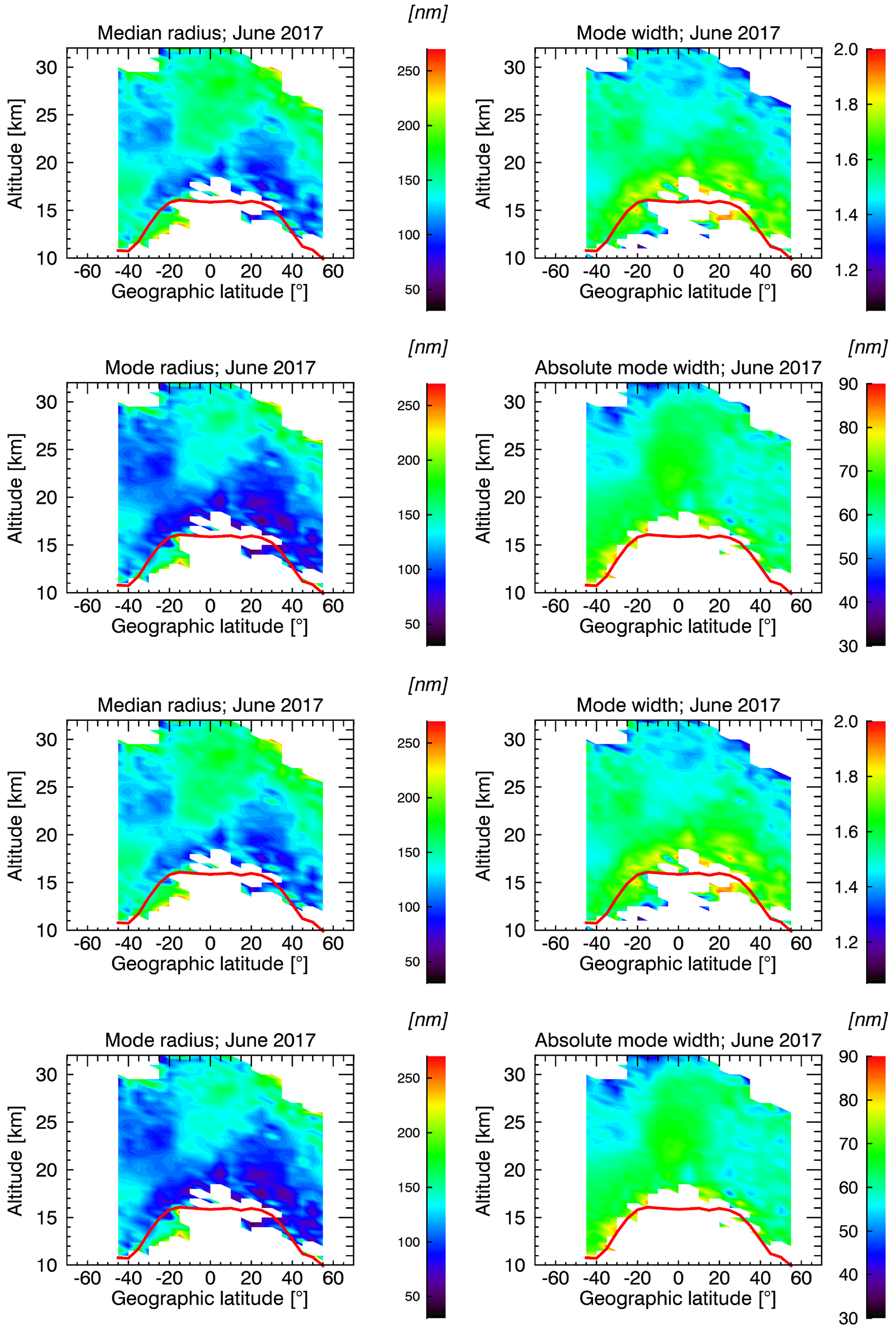
Figure 6 Monthly means of median radius, mode width, mode radius, absolute mode width, extinction coefficient at 449 nm, extinction ratio at 449 and 756 nm, number density and effective radius for June 2017 with 5^∘ latitude bins. The red line indicates tropopause height.

The month of June 2017 is chosen here because it shows the closest-to-background conditions of the stratospheric aerosol layer, unperturbed by recent volcanic eruptions or large biomass burning, that is observable in the time frame covered by the SAGE III/ISS measurements at the time of writing. It is important to note that, because of the slow latitude shift of the solar occultation measurements (see Fig. 1) due to the orbit of the ISS, there is a time shift in the contour plots shown in Fig. 6, i.e. the individual profiles correspond to different dates in the month of June 2017. This latitudinal shift, together with the low amount of solar occultation measurements that can be performed by SAGE III/ISS per day (around 30), also means that showing a higher temporal resolution would not give a better overview. This limits the possibility to observe temporal changes of the retrieved parameters over short time frames, e.g. shorter than a month.

The upper and lower boundaries of the colour bars in Fig. 6 roughly mark the ranges within which the values of the respective quantities fall for the data set between June 2017 and December 2019. The median values for this time frame at 20 km altitude are 130.6 nm for the median radius, 1.54 for the mode width σ, 108.6 nm for the mode radius, 62.4 nm for the absolute mode width ω, 3.17 cm⁻³ for the number density and 188.6 nm for the effective radius. The mode radius is always smaller, and the effective radius is always greater than the median radius. These results generally match stratospheric aerosol size distribution parameter retrieval results from other published works in magnitude. However, there is a limited amount of such work in the literature, which is not always directly comparable since different quantities are shown, which are often retrieved at different times and latitudes. For example, Bingen et al. (2004) and Fussen et al. (2001) find mode radii roughly between 200 and 600 nm in the aftermath of the Mount Pinatubo eruption in 1991, while in other works the mode radius generally stays smaller than 130 nm (Mclinden et al., 1999; Bourassa et al., 2008; Malinina et al., 2018). Median radii retrieved by Bourassa et al. (2008) lie roughly between 30 and 130 nm. The assumed mode widths σ can range from monodispersed or effectively 1.0 (Thomason et al., 2008) to 1.4 (Ugolnikov and Maslov, 2018) and 1.6 (Bourassa et al., 2008; Malinina et al., 2018).

Also stratospheric aerosol size distribution parameter retrievals from occultation measurements may lead to systematically larger particle sizes than retrievals from other optical methods, like lidar backscatter measurements, due to differences in the sensitivity of the measurement techniques to larger and smaller aerosols due to different scattering angles (von Savigny and Hoffmann, 2020). This may also, in part, explain differences between retrievals from occultation and limb measurements. In general, as can be seen in Fig. 3, the extinction efficiencies of Mie scattering particles at the wavelengths used are very low for radii lower than roughly 50 nm, which is why most optical measurements will struggle to obtain usable information about particles in that size range.

It should be noted that one of the major advantages of the retrieval method presented here, and using three wavelengths instead of two, is that the lookup table provides unique solutions for almost all of the extinction spectra that can plausibly be observed based on the assumptions made about the aerosol composition and its PSD, i.e. there is exactly one combination of median radius and mode width that can reproduce the spectral dependence of the extinction put in. This is not the case when using only two spectral channels, since then there is a multitude of possible PSD parameter combinations for a monomodal lognormal distribution that reproduce the same spectral pattern, while having very different median radii, as pointed out by Malinina et al. (2019), making it unclear which one best describes the true conditions in the atmosphere.

In the results of the current work, median radius and mode width show an anticorrelation at most latitudes and altitudes, which is at least in part because the mode width σ is defined relative to r_med. This means that, with an increasing median radius, a fixed absolute mode width ω corresponds to a decreasing σ. Also, an anticorrelation between the extinction ratio at 449 and 756 nm and the effective radius and the median radius and mode radius can be observed. This is to be expected since, in the wavelength range used in this work, smaller particles have larger Ångström exponents than larger particles, resulting in larger ratios of extinction coefficients at a smaller wavelength to a larger wavelength. Every contour plot shows a feature in the tropics roughly between 20 and 25 km, which could be remnants of the eruptions of the Calbuco volcano (41.3^∘ S, 72.6^∘ W) on 22 and 23 April of 2015, which produced plumes reaching into the stratosphere (Romero et al., 2016). As is to be expected, the observable part of the Junge layer shifts in altitude, depending on latitude, being lower at higher latitudes.

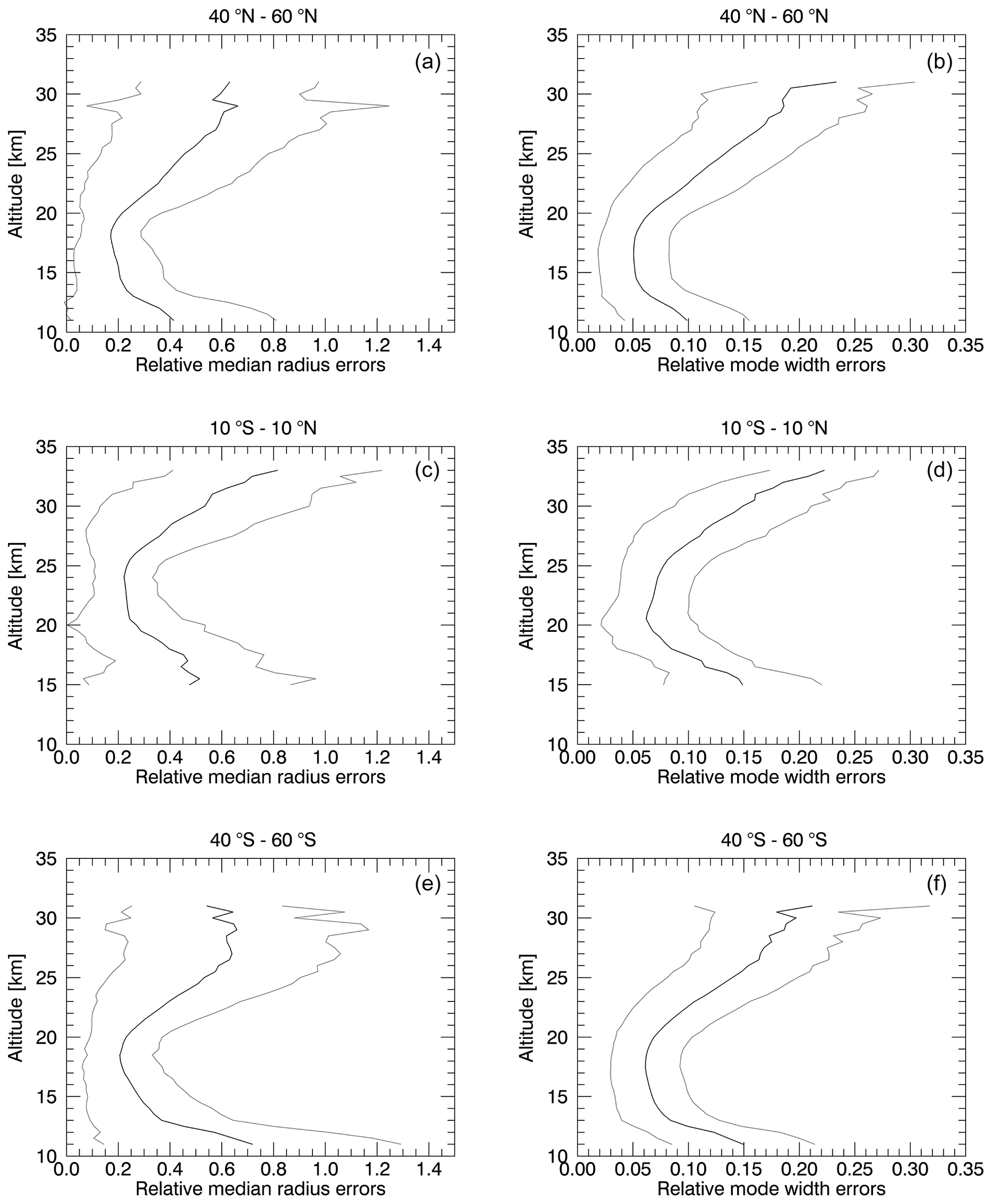
Figure 7 Relative total errors of median radius (a, c, e) and mode width (b, d, f) averaged over all measurements between June 2017 and December 2019 shown as black line. Averages are shown between 40 and 60^∘ N (a, b), 10^∘ S and 10^∘ N (c, d), and 40 and 60^∘ S (e, f). Grey lines indicate the standard deviation.

In Fig. 7, relative total errors of the median radius (left column) and mode width (right column) are shown. The total errors were calculated as explained in Sect. 4. The plots show temporal averages from June 2017 to December 2019 in different latitude bins. The top row shows averages between 40 and 60^∘ N, the middle row shows tropical averages between 10^∘ S and 10^∘ N, and the lower row depicts averages between 40 and 60^∘ S. The respective standard deviations are represented by grey lines. To have representative errors for the retrieval data produced, here also only values with corresponding accuracy parameters above 16 are considered.

In the peak area of the Junge layer, the relative total errors lie between 20 % and 25 % for the median radius and 5 % and 7 % for the mode width. At lower and higher altitudes, where the aerosols contribute less to the overall extinction of solar radiation and fewer measurements deliver analysable data, the errors and their standard deviations become larger. A perturbation of the real refractive index by 0.5 % to 0.6 % (see Sect. 4), depending on wavelength, resulted in relative uncertainties roughly between 3.5 % and 5 % for the median radius and 0.5 % to 1.3 % for the mode width. A perturbation of the imaginary part of the refractive index, as discussed in Sect. 4, resulted in relative uncertainties of roughly 0.4 % to 1 % for r_med and 0.15 % to 0.35 % for σ. These uncertainties are included in the relative total errors, which were described beforehand and are depicted in Fig. 7.

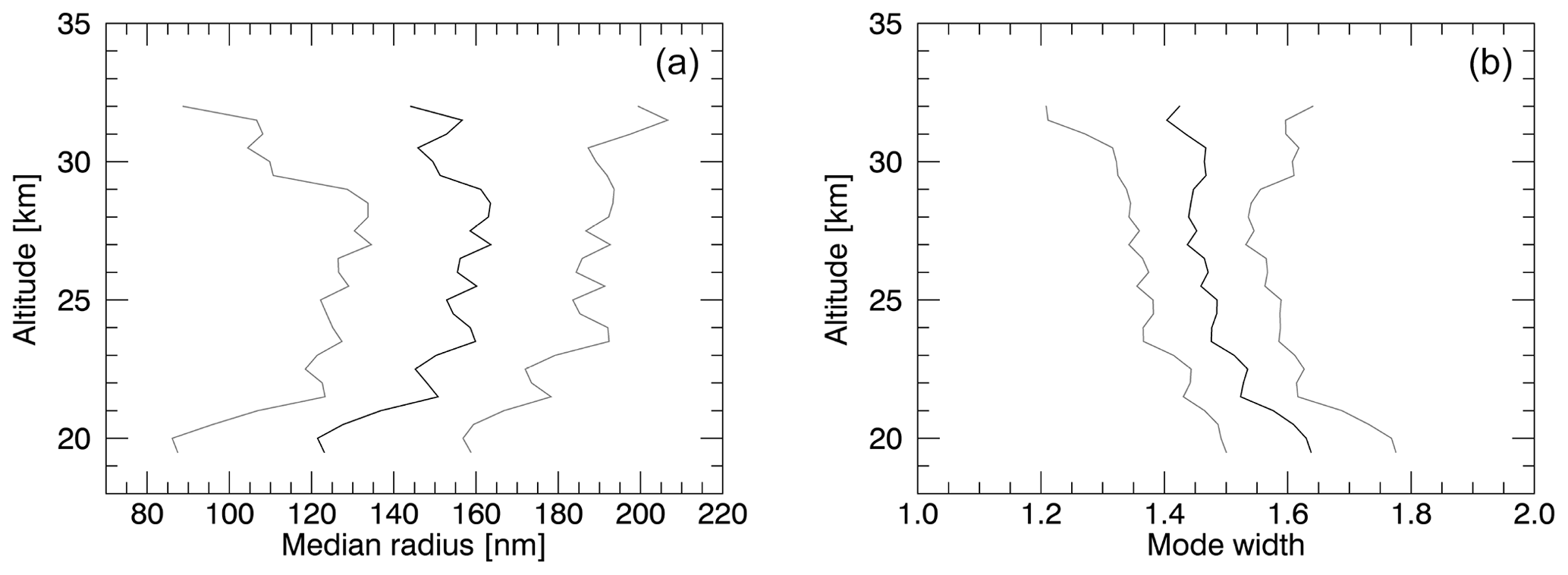
Figure 8 Profiles of median radius (a) and mode width (b) averaged between 2.5^∘ S and 2.5^∘ N for the month of June 2017. Grey lines depict total errors as calculated in Sect. 4.

In addition to the contour plots shown before, in Fig. 8 two exemplary vertical profiles of the median radius (Fig. 8a) and the mode width (Fig. 8b) are shown for easier reference of values. Just as in Fig. 6, the profiles contain averaged values for the month of June 2017. The latitude bin used here contains measurements between 2.5^∘ S and 2.5^∘ N, and the grey lines show the total errors, which were calculated as explained in Sect. 4. Here, only measurements with error ellipses lying completely within the set of curves used for the retrieval were used, as was also explained in Sect. 4.

Additionally, in Fig. 9, averaged relative differences between Ångström exponents at 449 and 756 nm calculated from the extinction coefficients from SAGE III/ISS and from extinction coefficients obtained with Mie calculations using the median radii and mode widths retrieved with the presented method are shown. This is a measure of the accuracy with which the retrieval algorithm assigns median radius and mode width values to the measurement data points via interpolation (see Fig. 4) and to what extent the Ångström law correctly describes the spectral dependence of the aerosol extinction. Please note that the uncertainties of the extinction measurements and, therefore, also the error bars play no role here. An even distribution of 5 % of the data between June 2017 and December 2019 is used for this calculation. The relative differences between the Ångström exponents calculated from the SAGE III/ISS data and the ones calculated with the retrieved size distribution parameters lie between −0.4 % and −0.08 %, which are very small and indicate an accurately working assignment of values in the aforementioned step of the retrieval. For the combinations of 756 and 1544 nm and 449 and 1544 nm, the differences are even slightly smaller.

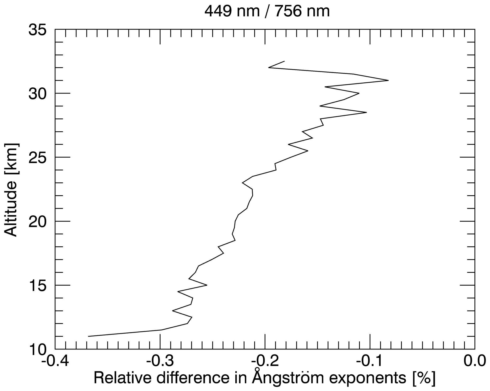
Figure 9 Temporal averages of relative differences between Ångström exponents at 449 and 756 nm from SAGE III/ISS and from Mie calculations with retrieved PSD parameters from June 2017 to December 2019 in percent.

6 Conclusions

In this work, a novel method for the determination of the size distribution parameters of stratospheric sulfate aerosols, based on the SAGE III/ISS solar occultation measurements, was implemented. The main purpose of the study is to demonstrate this retrieval technique. An analysis of the SAGE III/ISS data set will be presented in a future study.

Due to the wide spectral range covered by the SAGE III/ISS measuring instrument, the median radius r_med and mode width σ of the assumed monomodal lognormal distribution can be retrieved independently, without having to assume one of them beforehand. Also, using three wavelengths gives unique solutions for the PSD parameters, i.e. unique size distributions, for most atmospheric conditions that can plausibly be expected, which is not the case when using only two spectral channels. Both points are major advantages of this retrieval method over others. In addition, using occultation measurements has an advantage in that the extinction coefficients were obtained without the need for a priori assumptions about the aerosols. However, as discussed, satellite solar occultation measurements also come with the limitation of limited spatial and temporal coverage. In addition to r_med and σ, the number density, effective radius, mode radius as well as the absolute mode width have been calculated.

The aerosol particle size retrieval results are, of course, based on the assumptions about the PSD, but also dependent on the assumption of the particle composition, since real and imaginary refractive indices are needed for the Mie calculations. Here, the stratospheric aerosol are assumed to be pure H₂SO₄-H₂O-droplets, which may not be true at all times, e.g. after large biomass burning events (Murphy et al., 2007).

At the peak of the Junge layer, typical errors lie between 20 % and 25 % for the median radius and 5 % and 7 % for the mode width and increase at higher and lower altitudes. These errors are reasonable, especially since the real errors are very likely smaller, since the extinction coefficients of the different spectral channels of SAGE III/ISS are not completely independent as it was assumed in this work. Also, a comparison between Ångström exponents calculated from the SAGE III/ISS aerosol extinction coefficients and from extinction coefficients calculated with a Mie code, using the retrieved size distribution parameters, shows differences smaller than 0.5 %. Both this Ångström exponent comparison and the low-to-moderate errors of r_med and σ suggest that this retrieval technique is a solid tool for retrieving aerosol size distribution information from the SAGE III/ISS solar occultation measurements. The data produced in this way can be valuable for comparisons between measurement retrievals and model calculations as well as for the investigation of the impact of volcanic eruptions on climate and atmospheric chemistry.