Understanding balloon-borne frost point hygrometer measurements after contamination by mixed-phase clouds

Balloon-borne water vapour measurements in the upper troposphere and lower stratosphere (UTLS) by means of frost point hygrometers provide important information on air chemistry and climate. However, the risk of contamination from sublimating hydrometeors collected by the intake tube may render these measurements unusable, particularly after crossing low clouds containing supercooled droplets. A large set of (sub)tropical measurements during the 2016–2017 StratoClim balloon campaigns at the southern slopes of the Himalayas allows us to perform an in-depth analysis of this type of contamination. We investigate the efficiency of wall contact and freezing of supercooled droplets in the intake tube and the subsequent sublimation in the UTLS using computational fluid dynamics (CFD). We find that the airflow can enter the intake tube with impact angles up to 60^∘, owing to the pendulum motion of the payload. Supercooled droplets with radii > 70 µm, as they frequently occur in mid-tropospheric clouds, typically undergo contact freezing when entering the intake tube, whereas only about 50 % of droplets with 10 µm radius freeze, and droplets < 5 µm radius mostly avoid contact. According to CFD, sublimation of water from an icy intake can account for the occasionally observed unrealistically high water vapour mixing ratios (${\mathit{\chi }}_{{\mathrm{H}}_{\mathrm{2}}\mathrm{O}}$ > 100 ppmv) in the stratosphere. Furthermore, we use CFD to differentiate between stratospheric water vapour contamination by an icy intake tube and contamination caused by outgassing from the balloon and payload, revealing that the latter starts playing a role only during ascent at high altitudes (p < 20 hPa).

1 Introduction

Sources of contamination for cryogenic frost point hygrometers are water vapour outgassing from the balloon envelope, the parachute, the nylon cord, or sublimation of hydrometeors collected in the intake tube of the instrument (Hall et al., 2016; Vömel et al., 2016). These are contamination sources common to all balloon-borne water vapour measurement techniques (Goodman and Chleck, 1971; Vömel et al., 2007c; Khaykin et al., 2013). The relative impact of contamination on the measurements in the stratosphere is severe since the environmental water vapour mixing ratios are 2–3 orders of magnitude smaller than in the troposphere. Over time, contamination by the flight train (balloon, parachute, nylon cord) has been reduced by increasing the length of the cord by means of an unwinder and by giving preference to descent over ascent data (Mastenbrook and Dinger, 1961; Mastenbrook, 1965, 1968; Mastenbrook and Oltmans, 1983; Oltmans and Hofmann, 1995; Vömel et al., 1995; Oltmans et al., 2000; Khaykin et al., 2013; Hall et al., 2016). Standard lengths presently used are of the order of 50 to 60 m (Vömel et al., 2016; Brunamonti et al., 2018). The World Meteorological Organization recommends thin hydrophobic tethers longer than 40 m (WMO, 2018; Immler et al., 2010). Nevertheless, it has been shown (Kräuchi et al., 2016) that the balloon wake in combination with the swinging motion of the payload leaves a quasi-periodic signal even in the temperature measurements by radiosondes. Descent data are not always an option because some instrument intakes and control systems are optimized for ascent (Kämpfer, 2013).

The first water vapour measurements in the stratosphere were performed by means of a frost point hygrometer onboard an aircraft. The reported frost point temperature was about −83 ^∘C at 12 km height (Brewer et al., 1948). Frost point hygrometers were then developed for balloon-borne platforms. The first water vapour measurement from balloon-borne frost point hygrometers reported a frost point temperature of about −70 ^∘C at 15 hPa (Barret et al., 1949, 1950; Suomi and Barrett, 1952), corresponding to unrealistically high H₂O mixing ratios (> 100 ppmv). Later, Mastenbrook and Dinger (1961) used a new lightweight dew point instrument for frost point measurements in the stratosphere. For the first time, measures to minimize contamination of the air sample with moisture carried aloft by the balloon were mentioned. The instrument was carried about 275 m below the balloon assembly and the ascent data were accepted only if validated by the descent data. The descent was achieved by two methods: the use of a big parachute or the use of a tandem balloon assembly. Nowadays, controlled descent profiles are obtained by using a valve in the balloon neck (Hall et al., 2016; Kräuchi et al., 2016) that slowly releases gas from the balloon. Nearly all balloon-borne frost point hygrometer (FPH) soundings performed by NOAA's Global Monitoring Laboratory (Hall et al., 2016) use this valve.

Mastenbrook (1965, 1968) identified contamination by the instrument package as a source of the higher and more variable concentrations of water vapour at stratospheric levels. The surfaces of the sensing cavities and intake ducts were considered as a potential contamination source and redesigned using larger diameter stainless steel intake tubes that allow higher flow rates. These improvements enabled the instrument to measure typical stratospheric H₂O mixing ratios of about 4 ppmv. Mastenbrook (1966) started building fully symmetric instruments for ascent and descent. Mastenbrook and Oltmans (1983) paid particular attention to the intake tubes of the frost point hygrometer. These tubes are currently 2.5 cm in diameter and are made of 25 µm thick stainless steel (Vömel et al., 2007b). The tubes need to be thoroughly cleaned before flight. They extend above and below the instrument package by more than 15 cm, shielding the air flowing into the instrument from contamination by water outgassing from the instrument's Styrofoam box. The frost point temperature is measured at the mirror surface displaced 1.25 cm from the intake tube wall and placed at the centre of the tube, 17 cm from the opening of the intake tube.

New designs of frost point hygrometers such as the SnowWhite sonde from Meteolabor steered away from the intake tube design (Fujiwara et al., 2003; Vömel et al., 2003). However, the SnowWhite design was shown to be susceptible to the ingress of hydrometeors in the intake (Cirisan et al., 2014). Under supersaturated conditions, the intake duct was actively heated, with the intention to measure the total water content (TWC), i.e. gaseous plus particulate H₂O, instead of just gaseous H₂O mixing ratio, as claimed by the manufacturer (Vaughan et al., 2005). The SnowWhite sonde was also reported to measure saturation over ice in the troposphere of 120 %–140 %, which could not be modelled irrespective of the assumed scenario, leading Cirisan et al. (2014) to conclude the measurement was erroneous and likely created by contamination.

With the increasing miniaturization and ease of use, balloon-borne frost point hygrometers started to be employed more systematically at an increasing number of locations and under a wide range of meteorological conditions (Vömel et al., 2002, 2007b; Bian et al., 2012; Hall et al., 2016; Brunamonti et al., 2018), creating new challenges for the instrument. When passing through mixed-phase clouds with supercooled liquid droplets, the balloon and payload surfaces can accumulate ice, which will sublimate in the subsaturated environment of the stratosphere. Intake tubes might represent a susceptible surface for this type of contamination (Vömel et al., 2016).

Contaminated water vapour measurements in the stratosphere are a common feature when the troposphere is very moist, such as during deep convection in mid latitudes (the Asian and North American monsoons) and in the tropics (Holger Vömel, personal communication, 2016). Contamination requires a careful quality check of the Cryogenic Frost point Hygrometer (CFH) data, representing a source of uncertainty, especially in the lower stratosphere. This artifact can also lead to systematic biases, as it makes the operator prefer dryer launching conditions, which can affect satellite validation procedures and climatological records (Vömel et al., 2007a).

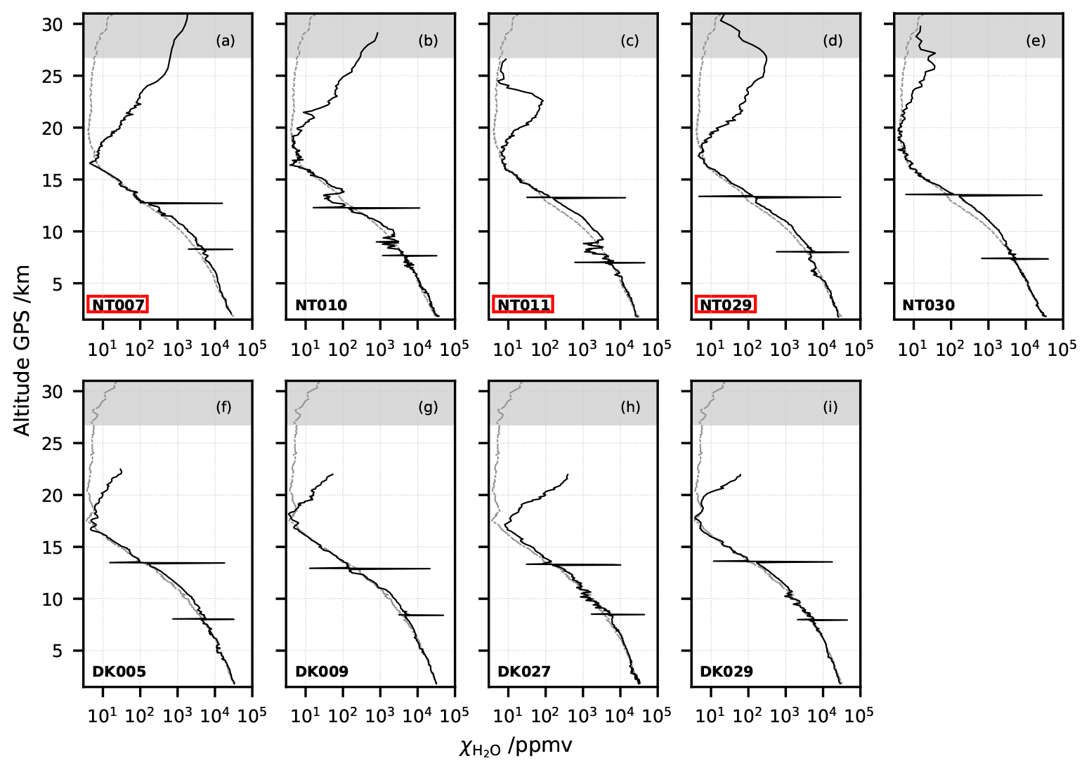
Figure 1 Nine water vapour mixing ratio profiles from the CFH showing contaminated values in the stratosphere (out of 43 profiles taken during StratoClim 16/17). (a–e) Campaign in Naintal (NT), India, summer 2016. (f–i) Campaign in Dhulikhel (DK), Nepal, summer 2017. Black lines: measured individual profiles. Grey lines: respective campaign season average (mean of 22 (NT) or 7 (DK) profiles), excluding the individual profiles presented here as contaminated, as shown in Brunamonti et al. (2018). Grey shading highlights possible balloon contamination above the 20 hPa level in the season average. Two spikes per profile: instrumental clearing and freezing cycles. Highlighted in red: three night-time launches with the CFH and the COBALD, which are further investigated in this study.

During the 2016–2017 StratoClim balloon campaigns at the southern slopes of the Himalayas, 43 out of a total of 63 soundings carried water vapour measurements by means of the CFH (see Vömel et al., 2007b, 2016), and of these 9 showed strongly contaminated water vapour measurements in the stratosphere. These nine soundings are shown in Fig. 1 (see also grey points in Fig. 2 of Brunamonti et al., 2019). The contaminated profiles of the CFH soundings are displayed by black lines, while the season average profile, excluding the contaminated profiles, as shown in Brunamonti et al. (2018) are shown by the grey line. Above 20 hPa the season average profile is also considered contaminated, possibly due to water outgassing from the balloon envelope. The values are nonetheless shown in Fig. 1 and marked with grey shading. Three of the nine contaminated CFH soundings also carried the COmpact Backscatter AerosoL Detector (COBALD) (Wienhold, 2008), namely NT007, NT011 and NT029.

Here, we analyse these three soundings thoroughly for contamination due to supercooled droplets impacting inside the intake tube during mixed-phase clouds and subsequent sublimation of the formed ice layer in the upper troposphere and lower stratosphere (UTLS). We also investigate the balloon envelope and instrument box as possible sources of contamination. In Sect. 2, we present the dataset and instruments and analyse the mixed-phase clouds. In Sect. 3, we describe balloon trajectories and estimate the impact angles of supercooled droplets onto the tops of the intake tubes. Section 4 introduces the computational fluid dynamic (CFD) tool FLUENT by ANSYS (2012). In Sect. 5, we present the results of the different CFD studies, namely Sect. 5.1 for the freezing efficiency of supercooled droplets; Sect. 5.2 for the CFD-based description of the sublimation process and the evolution of the ice layer; Sect. 5.3 for the implications for the measurements in the upper troposphere; and Sect. 5.4 for the simulation of the contamination stemming from the balloon envelope and instrument packaging. Finally, Sect. 6 provides design and operation recommendations to decrease the effect of contamination.

2 StratoClim balloon campaigns

Brunamonti et al. (2018) offer an overview of the instrumentation and dataset collected during the 2016–2017 StratoClim balloon campaigns at the southern slopes of the Himalayas, deriving a comprehensive understanding of the morphology and large-scale dynamics of the Asian Summer Monsoon Anticyclone (ASMA). Here, we focus on humidity measurements in the upper troposphere and lower stratosphere region, including the measurement of mixed-phase and ice clouds, and provide brief instrument descriptions.

2.1 CFH and RS41 water vapour measurements

The two instruments measuring water vapour content in this study were the radiosonde RS41-SGP (hereinafter referred to as “RS41”) manufactured by Vaisala, Finland (Vaisala, 2013), and the Cryogenic Frost point Hygrometer, CFH (Vömel et al., 2007c, 2016), manufactured by ENSCI (USA). The RS41 measures relative humidity (RH) by means of a thin-film capacitive sensor (Jachowicz and Senturia, 1981) with a nominal uncertainty in soundings of 4 % for temperature T > −60 ^∘C (Vaisala, 2013). In this study, we used corrected RH data provided by the Vaisala MW41 software for the RS41 measurement, which implements an empirical time lag correction, accounting for the operation of the capacitive sensor under heated conditions by ΔT = 5 K above ambient temperature and correcting for irregularities determined by the zero humidity automated ground check (Vaisala, 2013). In contrast to the RS41, the CFH measures the frost point temperature (T_frost). It controls the reflectance of a dew or frost layer on a mirror by heating against continuous cooling of the mirror by a cryogenic liquid. When the dew or frost layer is in equilibrium with the air flowing past the mirror, i.e. neither growing nor evaporating, it is by definition at the dew point or frost point temperature, which is a direct measure of the H₂O partial pressure in the gas phase. The uncertainty of the CFH has been estimated to be smaller than 10 % in water vapour mixing ratio up to approximately 28 km altitude (Vömel et al., 2007c, 2016).

The performance of the two instruments during the 2016–2017 StratoClim balloon campaigns has been thoroughly compared, and dry biases of 3 %–6 % (0.1–0.5 ppmv) for 80–120 hPa and 9 % (0.4 ppmv) for 60–80 hPa of the RS41 compared to the CFH were found. The study uses Vaisala-corrected RS41 RH measurements (Brunamonti et al., 2019). These were campaign mean results, whereas flight-by-flight discrepancies as large as 50 % did occur. In previous publications of this dataset (Brunamonti et al., 2018, 2019), contaminated measurements in the stratosphere were discarded using an empirical threshold. In particular, all data above the cold-point tropopause (CPT) were flagged as contaminated if H₂O mixing ratios exceeded 10 ppmv at any altitude in the stratosphere. In addition, all data at pressures below 20 hPa were also discarded, due to suspected contamination by the balloon or payload train. With decreasing pressures starting above about the 60 hPa level, all the RS41 measurements showed an unrealistic increase in H₂O mixing ratios up to several tens of ppmv (Brunamonti et al., 2019). We did not consider this behaviour to be due to contamination, as the capacitive sensor of the RS41 is constantly heated to 5 ^∘C warmer than ambient air, preventing icing of the sensor in supercooled clouds and supersaturation conditions. Rather, the capacitive sensor has poor sensitivity at low RH values in a cold environment. In contrast to Brunamonti et al. (2018, 2019), here we did not remove the CFH clearing and freezing cycles (Vömel et al., 2016), which occurred twice per flight. The clearing and freezing cycle consists of a forced heating of the CFH mirror to blow off any deposit, followed by a forced cooling of the mirror. During the cycle at approximately −15 ^∘C, the mirror is forced cooled to temperatures below which ice certainly forms ($<-\mathrm{40}$ ^∘C). During the second cycle at approximately −53 ^∘C, the mirror is forced cooled to temperatures below which hexagonal ice forms ($<-\mathrm{82}$ ^∘C). Hexagonal ice is more stable than cubic ice. The data collected during the freezing and clearing cycles are not used for further analysis, but we do not remove them from the water vapour profiles. This feature gives us confidence that after it the phase of the deposit in the mirror was ice or hexagonal ice.

We compared the dew- and frost-related quantities (dew and frost points, corresponding RHs, mixing ratios) of the CFH and RS41 as follows. The ice saturation ratio S_ice, i.e. relative humidity with respect to ice, was calculated using the frost point temperature measured by the CFH, the air temperature measured by the RS41, and the parameterization for saturation vapour pressure over ice by Murphy and Koop (2005), while relative humidity with respect to liquid water (S_liq,RS41, also sometimes simply termed “RH”) was directly measured by the RS41. We also present relative humidity (S_liq) computed from the CFH frost point temperature, the RS41 air temperature and the parameterization for saturation vapour pressure over water by Murphy and Koop (2005). S_liq,d considers the deposit on the CFH mirror to be dew, i.e. liquid water, and S_liq,f considers the deposit to be frost, i.e. ice. Water vapour mixing ratio (χ_CFH) in ppmv from the CFH was calculated from the frost (or dew) point temperature, the air pressure from the RS41 and the parameterization for saturation vapour pressure over ice (or liquid water) by Murphy and Koop (2005). The water vapour mixing ratio in ppmv derived from the RS41 (χ_RS41) uses the relative humidity, air temperature, and air pressure from the RS41 and the parameterization for saturation vapour pressure over water by Hardy (1998) as used by Vaisala (2013).

All data presented were taken during balloon ascent, because this was the part of the flight affected by contamination. We averaged all data in 1 hPa intervals (bins) from the ground to the burst altitude. The downward-looking intake did not get contaminated by hydrometeors during mixed-phase cloud traverses. However, we preferred ascent over descent because the instrument's descent velocity in the stratosphere was very high, up to 50 m s⁻¹, which might have caused controller oscillations and yields measurements at much lower vertical resolution than during ascent. We show below that it is important to consider payload pendulum oscillations to explain certain features in the humidity measurements. For their analysis we used 1 s GPS data retrieved from the RS41. We also used GPS altitude as the main vertical coordinate for all instruments. The ascent velocity (w) in m s⁻¹ and latitude and longitude are taken directly from the RS41 GPS product.

2.2 COBALD backscatter measurements

In StratoClim, we performed a total of 43 balloon soundings with the CFH and the RS41; 20 of these were performed at night also carrying the COBALD, so that liquid and ice clouds in the lower and middle troposphere could be detected. The COBALD can only be flown at night because daylight saturates the photodetector (Cirisan et al., 2014).

The COBALD data are expressed as backscatter ratio (BSR), i.e. the ratio of the total-to-molecular backscatter coefficients. This is calculated by dividing the total measured signal by its molecular contribution, which is computed from the atmospheric extinction according to Bucholtz (1995) and using air density derived from the measurements of temperature and pressure. The COBALD BSR uncertainty as inferred by this technique is estimated to be around 5 % (Vernier et al., 2015). For the backscatter data analysis, we also present the colour index (CI). CI is defined as the 940-to-455 nm ratio of the aerosol component of the BSR, i.e. $\mathrm{CI}=({\mathrm{BSR}}_{\mathrm{940}}-\mathrm{1})/({\mathrm{BSR}}_{\mathrm{455}}-\mathrm{1})$. CI is independent of the number density; therefore, it is a useful indicator of particle size as long as particles are sufficiently small, so that Mie scattering oscillations can be avoided, namely radii smaller than 2–3 µm. From this, one obtains CI < 7 for aerosol and CI > 7 for cloud particles (Cirisan et al., 2014; Brunamonti et al., 2018).

The CFH–COBALD combination is a powerful tool to investigate cirrus clouds. Although the estimation of ice water content (IWC) from the COBALD BSR measurements with just two wavelengths – 455 and 940 nm – is quite uncertain without additional information about the ice crystal size or distribution, IWC can be constrained for thin cirrus clouds (Brabec et al., 2012). The retrieval of mean particle size is a matter of size distribution complexity: if the distribution is simple, as is the case for stratospheric aerosol, the mode radius can be estimated from the colour index (Rosen and Kjome, 1991). In this work, however, we were interested in relatively thick mixed-phase clouds as observed in tropical convection (Wendisch et al., 2016; Cecchini et al., 2017). The backscatter from dense mixed-phase clouds may saturate the COBALD. In this context, it was hard to retrieve more information from the COBALD than the vertical thickness of these clouds and the indication whether they were purely ice (CI ∼ 20) or not.

2.3 Flight NT011

We discuss results of the analysis for sounding NT011 in the main body of this paper and the results for NT029 and NT007 in the Supplement. Figure 2 shows the vertical profile of NT011 measured on 15 August 2016 in Nainital. Figure 2a displays the air temperature from the RS41, S_liq,RS41 from the RS41, calculated ice saturation ratio S_ice from the CFH and calculated water saturation ratio S_liq,d and S_liq,f from the CFH; note that the condensate on the CFH mirror was forced to turn from dew to frost after the freezing cycle, at T_frost = −15 ^∘C. Figure 2b shows the H₂O mixing ratio, ${\mathit{\chi }}_{{\mathrm{H}}_{\mathrm{2}}\mathrm{O}}$ (χ_CFH) and the Nainital campaign mean excluding the contaminated CFH measurements (〈χ_CFH〉). Both panels (a) and (b) show 1 s data to illustrate the signal-to-noise ratio (S∕N) of the CFH water vapour measurements. Figure 2c shows the COBALD BSR at 940 nm, BSR at 450 nm and CI.

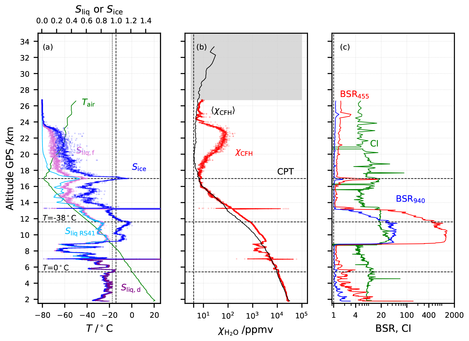
Figure 2 Flight NT011 in Nainital, India, on 15 August 2016. Lines: 1 hPa interval-averaged values. Dots: 1 s data. (a) Green: air temperature from the Vaisala RS41; light blue: saturation over water (S_liq,RS41) measured by the RS41; blue: ice saturation (S_ice) from the CFH; purple: saturation over water (S_liq,d) from the CFH considering the deposit on the mirror to be dew; pink: saturation over water (S_liq,f) from the CFH considering the deposit on the mirror to be frost. Note that the condensate on the CFH mirror was forced to turn from dew to frost after the freezing cycle, at T_frost = −15 ^∘C. (b) Red: H₂O mixing ratio from the CFH in ppmv; black: season average H₂O mixing ratio excluding contaminated CFH profiles for the Nainital 2016 summer campaign (Brunamonti et al., 2018). Highlighted values with grey shading above the 20 hPa level are possibly contaminated by outgassing from the balloon envelope. “CPT” marks the cold point tropopause. (c) Red: 940 nm backscatter ratio from the COBALD; blue: same for 455 nm; green: colour index (CI) from the COBALD.

The lower stratospheric water vapour mixing ratios were unrealistically large, due to contamination, becoming visible right above the CPT but returning to values similar to those observed for the season average by the CFH excluding contaminated profiles (black line – Fig. 2b) below the balloon burst at 27 km altitude. The COBALD identified two clouds, one very thin cirrus cloud directly below the CPT (T_air= −78 ^∘C) and another geometrically and optically thick cloud in the range 9 to 13 km altitude and T_air= −20 ^∘C to T_air= −50 ^∘C. The lower cloud has S_liq< 1 and is sufficiently cold that the presence of liquid water is unlikely (Korolev et al., 2003). However, the CI observed between 9 and 10 km altitude supports the existence of liquid in this cloud at these altitudes, with air temperature between −20 and −25 ^∘C. Ice clouds are characterized by a very regular CI of about 20 with large ice particles, as evidenced in this cloud above 11 km altitude (see also Fig. 10f in Brunamonti et al., 2018). CI around 30 stems from the Mie oscillations in the transition regime and thus from the presence of smaller and more monodispersed scatterers, most likely supercooled cloud droplets. Additionally, the BSR ∼ 1000 at 940 nm was about as high as can be observed with the COBALD before the instrument would go into saturation. As indicated in Fig. 2, only the lowermost 750 m of the cloud provided evidence for the existence of supercooled droplets at temperatures between −20 and −25 ^∘C.

2.4 Modelling of mixed-phase clouds

The existence of liquid droplets in water-subsaturated clouds at these temperatures (T_air= −20 ^∘C) is unusual. However, the passage through an ice cloud would not cause the observed contamination. The ice crystals likely bounce off the surfaces of the balloon, payload and intake tube. The presence of supercooled liquid droplets is necessary to form the ice layer inside the intake tube. Only supercooled liquid droplets freeze upon contact with a surface and lead to an icy surface coating of the balloon, payload and intake tube.

Subsequently, we asked whether the balance between the different water phases described by the Wegener–Bergeron–Findeisen process (Pruppacher and Klett, 1997; Korolev et al., 2017) would provide enough time for the flights to encounter supercooled liquid droplets at these high altitudes and low temperatures. Could the observed water and ice saturation conditions in NT011 from 9.25 to 10 km altitude and at air temperatures of about ∼ −20 ^∘C support liquid droplets? What would their size distribution look like and how long would they survive?

Figure 3 shows the air temperature, the balloon ascent velocity, the saturation ratios S_ice and S_liq,f relative to ice and supercooled water from the CFH, respectively, and the S_liq from the RS41, as well as the 940 nm BSR and CI for the mixed-phase cloud region of flight NT011. Similar figures for flights NT029 and NT007 can be found in the Supplement (Figs. S2 and S10). The lower part of the cloud (9.25–10 km) showed 5 %–10 % ice supersaturation and 10 %–15 % subsaturation over water. This represented an unstable situation as the ice crystals grew at the expense of the liquid droplets, eventually resulting in a fully glaciated cloud with S_ice=1 (Korolev et al., 2017). At altitudes above 10 km, the balloon encountered S_liq < 0.8; i.e. liquid droplets were likely fully evaporated.

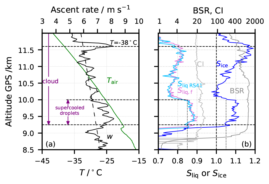
Figure 3 Mixed-phase cloud detail of flight NT011. Lines: 1 hPa interval-averaged values. (a) Green: air temperature; black: ascent velocity measured by the RS41 in m s⁻¹. (b) Light blue: saturation over water (S_liq,RS41) measured by the RS41; pink: saturation over water (S_liq,f) from the CFH considering the deposit on the mirror to be frost; blue: ice saturation (S_ice) from the CFH; dark grey: 940 nm backscatter ratio from the COBALD; light grey: colour index (CI) from the COBALD. Horizontal dashed lines mark the supercooled droplet region and T_air = −38 ^∘C.

In order to estimate the glaciation time (τ_g), the time it would take for the mixed-phase cloud to became an ice cloud, we applied a simple evaporation model based on the solution of the diffusion equation for diffusive particle growth or evaporation:

$$\begin{array}{}\text{(1)}& {\displaystyle \frac{\mathrm{d}{r}^{\mathrm{2}}}{\mathrm{d}t}}=\mathrm{2}{V}_{{\mathrm{H}}_{\mathrm{2}}\mathrm{O}}{D}_{\mathrm{g}}{n}_{\mathrm{g}}\left(S-\mathrm{1}\right),\end{array}$$

where r is the droplet or ice particle radius, $V_{{\mathrm{H}}_{\mathrm{2}}\mathrm{O}}$ is the volume of a H₂O molecule in the condensed phase (liquid or ice), D_g is the diffusivity of H₂O molecules in air, n_g is the number density of H₂O molecules in the gas phase, and S is the saturation ratio of water vapour over liquid water or ice. Equation (1) is a simplified form of Eqs. (13)–(21) of Pruppacher and Klett (1997). The results of the simulations are presented in Fig. 4.

Figure 4 Modelling of the Wegener–Bergeron–Findeisen process in mixed-phase cloud demonstrating that flight NT011 likely encountered supercooled liquid droplets. Solid lines: lower estimate of liquid water content (LWC). Dashed lines: upper estimate (see text). Initial size distributions for lower estimate simulation: n_ice = 0.02 cm⁻³, r_ice = 10 µm; n_liq,1 = 10 cm⁻³, r_liq,1 = 10 µm; n_liq,2 = 0.003 cm⁻³, r_liq,2 = 100 µm. Initial size distributions for upper estimate simulation are identical but with 50 % larger n_liq,1 and n_liq,2. (a) Blue lines: ice water content (IWC); purple lines: LWC; (b) blue lines: ice saturation ratio (S_ice); purple lines: liquid water saturation ratio (S_liq) for lower and upper estimates. Glaciation times of small droplets τ_g,1 ∼ 6 min, of big droplets τ_g,2 ∼ 17 min. Shaded-saturated ratios: observed ranges from Fig. 3. Vertical arrows: time when smaller liquid droplets fully evaporated. The computed time interval with S_ice and S_liq matching flight observations is Δt ∼ 7 min.

We modelled the Bergeron–Findeisen process in these clouds by applying Eq. (1) to both the evaporating droplets (S_liq < 1) and the growing ice crystals (S_ice > 1). We chose the size distribution of the liquid droplets to be bimodal in order to approximate in situ observations of broad droplet spectra in mixed-phase clouds (Korolev et al., 2017), with small liquid droplets r_liq,1 = 10 µm, n_liq,1 = 10 cm⁻³ and big liquid droplets r_liq,2 = 100 µm, n_liq,2 = 0.003 cm⁻³. We considered the number density of ice crystals to be consistent with ice nucleation particles (INP) at about 0.02 cm⁻³ (DeMott et al., 2010), neglecting secondary ice production processes, which might have enhanced ice number densities (Lawson et al., 2017) but would be highly uncertain. During the evolution of the mixed phase under the conditions characteristic for the lower end of the cloud in NT011 (9.25–10 km), the many small liquid droplets evaporated first, providing favourable conditions for the fewer large droplets, which would have needed about 20 min to finally evaporate; see Fig. 4.

Table 1 Lower cloud edge, thickness of cloud fraction containing supercooled liquid droplets, and estimated liquid water content (LWC) in mixed-phase clouds for flights NT007, NT011 and NT029.

The low concentration of ice crystals and the bimodality of the liquid droplet distribution allowed the bigger droplets to exist for a relatively long period of time in a mildly subsaturated environment (S_liq ∼ 0.90–0.85). For the simulation, we assumed two different initial distributions: a lower and an upper estimate of liquid water content (LWC); see Table 1. The lower estimate was constrained by the amount of ice required to sublimate in the stratosphere from the CFH intake tube in order to explain the observed contamination as determined by the computational fluid dynamics simulations discussed in the next sections. The upper estimate was determined such that it would provide the sum of the amount of ice sublimated in the stratosphere plus the amount sublimated in the upper troposphere, the latter computed from the difference between χ_RS41 and χ_CFH. These estimates are discussed more thoroughly in Sect. 5.2 and 5.3.

In Fig. 4, we see that both simulations for lower and upper estimates showed glaciation times of a smaller droplet mode of τ_g ∼ 6 min and of the bigger droplet mode of τ_g ∼ 17 min. The overlap with the range of observed S_liq and S_ice lasted for about 7 min, demonstrating that the cloud at 9.25–10 km in NT011 may have contained sufficient supercooled liquid to explain the contamination.

Flights NT029 and NT007 showed very similar cold mixed-phase clouds in terms of temperature, extent, and altitude to the mixed-phase cloud in NT011. These clouds also fulfilled the water (S_liq > 0.85) and ice (S_ice > 1.0) saturation and the COBALD CI (> 20) criteria of the mixed-phase cloud of NT011. Flight NT007 also showed a warmer mixed-phase cloud at lower altitude. The results of the simulation for flights NT029 and NT007 are shown in Figs. S3 and S11. Table 1 provides an overview of supercooled or mixed-phase cloud appearances in the three analysed soundings.

These simulations make a causal relationship between the mixed-phase cloud and the CFH intake contamination plausible. In addition, the updraft cores of cold clouds observed by Lawson et al. (2017) over the Colorado and Wyoming high plains support these assumptions, as these clouds did not experience secondary ice formation and significant concentrations of supercooled liquid in the form of small drops have survived temperatures as low as −37.5 ^∘C. Observed ice crystal number densities were lower than 4 cm⁻³ in clouds warmer than T_air= −23 ^∘C, increasing to 77 cm⁻³ at T_air= −25 ^∘C and to several hundred per cm⁻³ at even lower temperatures. Thus, some of the clouds described by Lawson et al. (2017) contained fewer ice particles and more supercooled droplets than the example treated here.

3 Balloon pendulum movement

As we show below by means of computational fluid dynamics (CFD) simulations, the passage through clouds containing supercooled water leads to hardly any collisions of the droplets with the walls of the intake tube, if the airflow is parallel to the walls. Under those conditions, only the mirror holder which is perpendicular to the airflow and extends into the intake tube causes collisions of larger droplets. Below the mirror holder, a recirculation cell might also cause some of the smaller droplets to collide; however, this would hardly affect the humidity measurement on the mirror. The situation changes dramatically when the air enters the intake tube at a non-zero angle, as would happen when pendulum oscillations and circular movement of the balloon payload induce a component of the payload motion perpendicular to the tube walls. Such pendulum oscillations and circular movement have been documented in the literature (e.g. Kräuchi et al., 2016). Here, we approximated the balloon plus payload by a two-body system connected by a weightless nylon cord and quantified the oscillations in terms of the instantaneous displacement of the payload from the balloon path. We then used the displacement to calculate the tilt of the payload relative to the flow and used the tilt angle and the associated horizontal velocity of the payload to quantitatively estimate the internal icing of the intake tube.

3.1 Pendulum oscillations derived from GPS data

We isolated the payload oscillations in relation to the balloon by removing the averaged trajectory of the payload. Figure 5a shows the horizontally projected trajectory of NT011, travelling first about 10 km northward in the troposphere and then about 40 km westward in the stratosphere before the balloon burst. The thick pink line shows the part of the trajectory, where the sonde flew through the cloud containing supercooled droplets, between 9.25 and 10 km altitude (see Fig. 3). The contamination happened most likely in this segment of the flight.

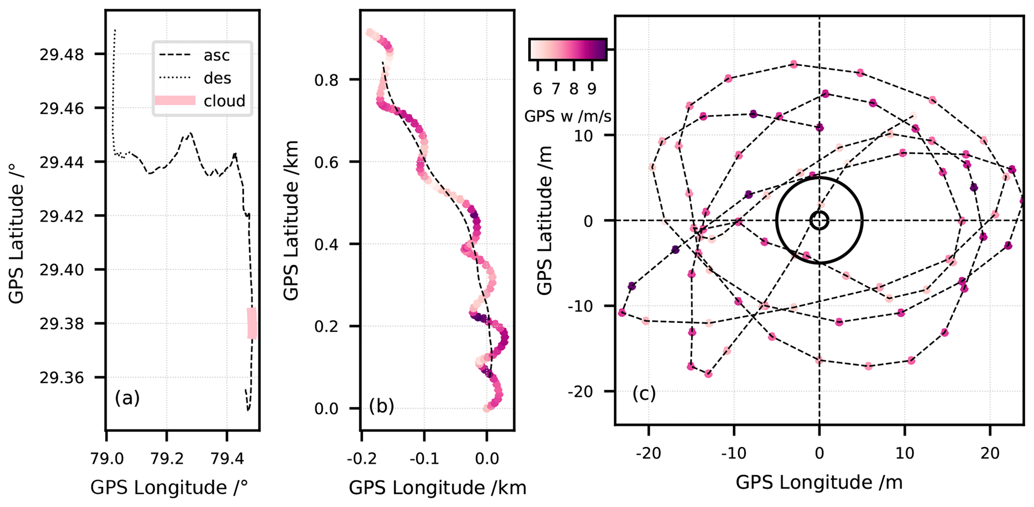
Figure 5 Pendulum analysis for the section of flight NT011 traversing the mixed-phase cloud. (a) Payload trajectory for the entire flight: ascent (dashed), descent (dotted) and mixed-phase cloud between 9.25 and 10 km altitude (thick pink line). (b) Zoom-in on the mixed-phase cloud with 1 s GPS data of payload trajectory (symbols) and derived balloon trajectory (dashed). (c) Detrended payload oscillations; approximate balloon sizes on the ground (r = 1 m) and at burst (r = 5 m) are shown by two circles. Colour code in panels (b) and (c): balloon ascent velocity.

Figure 5b zooms in on this cloudy section¹, showing the 1 s GPS data colour-coded by the ascent velocity in m s⁻¹. Figure 5c shows the residual payload motion relative to the balloon after “detrending”, i.e. subtracting the average trajectory of the payload. We obtained the average payload trajectory or balloon trajectory by smoothing the payload trajectory with a moving average corresponding to the pendulum oscillation period, which we evaluated by two independent methods. First, we considered the ideal pendulum oscillation frequency, $\mathit{\omega }=(g/L{)}^{\mathrm{1}/\mathrm{2}}$, where L is the length of the pendulum, in our case 55 m and g = 9.81 m s⁻². This yielded the oscillation period $\mathit{\tau }=\mathrm{2}\mathit{\pi }/\mathit{\omega }$ = 15 s. Second, we confirmed this result by means of a fast Fourier transform (FFT) analysis on the latitude and longitude detrended time series; see Appendix A. We concluded that, independently of the moving average used to detrend the longitude and latitude used in the FFT, the oscillation period was τ∼ 16.6 s. The same analysis was done for the clouds in flights NT029 and NT007, and the results are shown in Figs. S4 and S12.

Figure 5c also provides information on the degree to which the balloon itself might contribute to the contamination. The approximate balloon sizes at launch and burst are depicted as circles with 1 and 5 m radius, respectively. The circular movement placed the payload typically far outside the balloon wake, only sporadically penetrating the wake. The lack of periodic signs of contamination rendered it unlikely that H₂O collected by the balloon's skin contributed to the observed contamination. However, this behaviour changed above ∼ 27 km altitude, where the H₂O partial pressure became sufficiently low and the swing and circular movement of the payload was also weaker, so that the balloon outgassing started to dominate over the natural signal, leading to a systematic contamination in virtually every sounding (see Sect. 5.4).

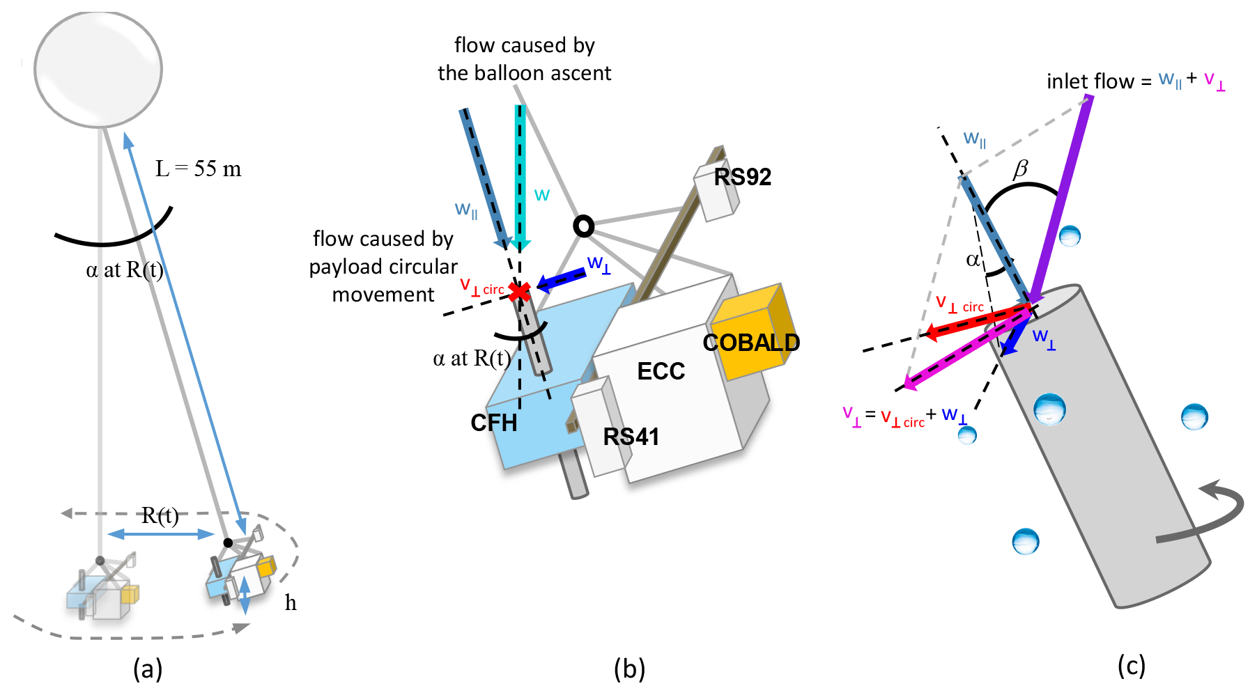
Figure 6 (a) Schematic of balloon and payload (not to scale). Payload is connected to the balloon by a 55 m long lightweight nylon cord. Payload oscillates with tilt angles α up to 25^∘ during ascent. (b) Schematic of payload with the two radiosondes (RS41 and RS92) and the three instruments (CFH, ECC Ozone and COBALD) and of intake flow geometry due to balloon ascent and payload circular movement. The flow caused by the vertical balloon ascent (w) has a component parallel to the intake tube (${\mathit{w}}_{\left|\right|}$) and a component perpendicular to the tube walls (w_⊥). Circular movement of the payload adds an additional component (${\mathit{v}}_{\perp ,\mathrm{circ}}$) in the plane perpendicular to the intake tube. (c) The total velocity perpendicular to the tube becomes ${\mathit{v}}_{\perp }={\mathit{v}}_{\perp ,\mathrm{circ}}+{\mathit{w}}_{\perp }$. The total perpendicular velocity v_⊥ and the parallel component of the ascent velocity to the intake tube ${\mathit{w}}_{\left|\right|}$ determine the inlet flow and the impact angle β.

Figure 6a shows a schematic of the balloon and payload as a two-body system and illustrates the displacement of the payload from under the balloon. From Fig. 5c we see that the radial displacement R of the payload in relation to the balloon position for flight NT011 was typically larger than 5 m (only 4 % of the measurements have R < 5 m). The corresponding tilt angle α is

$$\begin{array}{}\text{(2)}& \mathit{\alpha }\left(t\right)={\sin }^{-\mathrm{1}}\left({\displaystyle \frac{R\left(t\right)}{L}}\right)>\mathrm{5}{}^{\circ }.\end{array}$$

The maximum displacement was R_max ∼ 23 m, corresponding to a tilt angle α_max ∼ 25^∘. On average, 〈R〉 ∼ 15 m and 〈α〉 ∼ 16^∘, which represented a significant deviation from a flow through the tube parallel to the tube walls. The tilt angles α of the payload in the mixed-phase cloud of flight NT029 were of the same order of magnitude as the ones observed in the cloud of flight NT011, while for flight NT007 these were much smaller, almost half. We believe this difference stems from the different ascent velocities in the three flights.

Figure 6b shows how the flow through the CFH intake tube can be separated into flow parallel to the tube (${\mathit{w}}_{\left|\right|}$) and flow perpendicular to the tube (w_⊥). Figure 6b also shows how the different instruments are connected in the payload. The impact angle (β) of droplets onto the CFH intake tube was then partly determined by w_⊥ and ${\mathit{w}}_{\left|\right|}$ and consequently α. Moreover, the associated horizontal circular movement led to additional sideways impact, which we show to be even more important.

3.2 Impact angles derived from payload motion

Impact of droplets on the walls of the intake tube was forced by two effects that caused an airflow in the “horizontal plane”, i.e. the plane whose normal was the tube axis:

• i.

  the tube was tilted relative to the ascent flow, leading to the velocity ${\mathit{v}}_{\perp ,\mathrm{tilt}}={\mathit{w}}_{\perp }$;

• ii.

  the tube itself had a horizontal velocity ${\mathit{v}}_{\perp ,\mathrm{circ}}$ caused by the swinging or circular movement of the payload.

The vector sum of (i) and (ii) gave the total velocity perpendicular to the tube walls ${\mathit{v}}_{\perp }={\mathit{v}}_{\perp ,\mathrm{tilt}}+{\mathit{v}}_{\perp ,\mathrm{circ}}$; refer to Eq. (B4). Appendix B provides more details of the vector relations. In addition, we took into account the possibility of droplet impact on the mirror holder in the centre of the tube, even when the flow was perfectly aligned to the tube, but compared to (i) and (ii) this was a smaller contribution because larger droplets impacted already at the beginning of the tube and many of the smaller ones, which made it to the middle of the tube, were able to curve around the mirror holder and avoid contact.

Figure 5c shows that the residual motion of the payload resembles a circular motion with radius R = 15 m. Here, we only highlight the relevant magnitudes, but we provide a full treatment in Appendix B. The perpendicular velocity associated with the tube tilt ($w_{\perp }=v_{\perp ,\mathrm{tilt}}=w\sin \mathit{\alpha }$) can be determined from the tilt angle α and the ascent velocity w ∼ 7.5 m s⁻¹ (Fig. 3a). Equation (2) with R(t) = 15 m and L = 55 m yields α = 16^∘ and $v_{\perp ,\mathrm{tilt}}$ = 2.1 m s⁻¹. The perpendicular velocity associated with the payload circular movement (${\mathit{v}}_{\perp ,\mathrm{circ}}$) can be calculated from the difference between consecutive measurements after detrending based on the GPS position received every second. Figure 5c shows that $v_{\perp ,\mathrm{circ}}$ can be as big as 10 m s⁻¹ when the payload traverses the equilibrium point, straight below the balloon, or as small as 2 m s⁻¹ far from the equilibrium point. The circular movement of the payload leads to generally more impacts than the tilt of the tube. Here, the radially directed tilt contribution (2.1 m s⁻¹) and the circular progression added as the sum of orthogonal vectors increase the typical 5 m s⁻¹ circular speed (see Fig. 5c) to only 5.4 m s⁻¹, i.e. less than 10 %.

After accounting for the direction of movement when combining tilt and circular movement, the impact angle was calculated from the perpendicular velocities' sum (v_⊥) and the parallel component of the inlet flow (${\mathit{w}}_{\left|\right|}$) as shown in Fig. 6c. As the horizontal impact speed could be as high as 10 m s⁻¹, this corresponded to a maximum impact angle β = 53^∘. Such large impact angles are the reason why the CFH flying through mixed-phase clouds encounters a large risk of droplet collisions and freezing, accumulating potentially thick ice layers inside the intake tube, which renders further measurements in the stratosphere either impossible or possible only after a long recovery period of the instrument (i.e. until the ice sublimates). As a result from the full numerical treatment of the impacts in Appendix B, Fig. 7 shows the probability density functions (pdfs) of the magnitude of the perpendicular velocity (v_⊥) to the intake tube walls and of the parallel component of the ascent velocity (${\mathit{w}}_{\left|\right|}$) and the impact angle (β) as derived for the intake tube in the 9.25–10.0 km cloud section in flight NT011. Similar figures are shown for flights NT029 and NT007 in the Supplement. Perpendicular velocities were smaller for flight NT007 but, as the ascent velocity was also smaller in this flight, the impact angles were equivalent to those observed in flights NT011 and NT029.

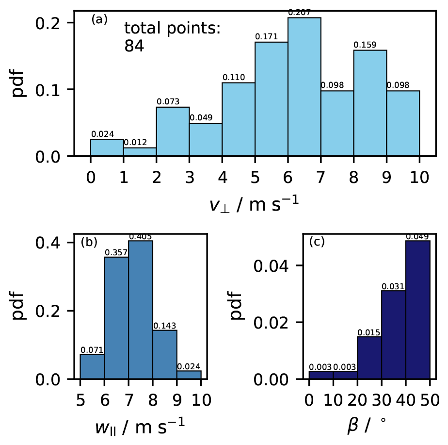
Figure 7 Probability density functions (pdfs) of impact parameters at the top end of the CFH intake tube during the passage through the mixed-phase cloud of flight NT011. (a) Velocity v_⊥ perpendicular to the tube walls; (b) velocity $w_{\left|\right|}$ parallel to the axis of the tube; (c) impact angle (β).

4 Computational fluid dynamic simulations

CFD tools have become commonly used in environmental studies, e.g. for error estimation of lidar and sodar Doppler beam swinging measurements in wakes of wind turbines (Lundquist et al., 2015), in new designs of photooxidation flow tube reactors (Huang et al., 2017), or to improve vehicle-based wind measurements (Hanlon and Risk, 2018). Here, we used CFD to estimate collision efficiencies of liquid droplets with different sizes encountering the CFH intake tube under various impact angles in order to understand first the ice build-up and second its sublimation from the icy intake to the passing airflow. We used the academic version of FLUENT and ANSYS Workbench 14.5 Release (ANSYS, 2012). FLUENT is a fluid simulation software used to predict fluid flow, heat and mass transfer, chemical reactions and other related phenomena. FLUENT has advanced physics modelling capabilities which include turbulence models, multiphase flows, heat transfer, combustion, and others. Here, FLUENT is used for the first time to investigate the operation of a balloon-borne instrument. For this study, the only feature not available was the water vapour pressure parameterization, which was added to the simulation through a user-defined function. For our study, we make most use of the ANSYS Workbench integrated approach from geometry to mesh to simulation to results visualization.

4.1 Geometry and mesh

By means of ANSYS Workbench, a mesh was developed mapping the intake tube geometry and providing the optimal geometric coverage. The CFH intake tube geometry was as described by Vömel et al. (2007c): a 2.5 cm diameter 34 cm long cylinder. The walls of the intake tube have a thickness of 25 µm but are approximated as infinitely thin. At the centre of the tube, the mirror holder is mapped by a cylinder extending 1.25 cm from the wall, oriented perpendicular to the flow. The mirror holder is 7 mm in diameter. The mirror is the base of the cylinder parallel to the flow at the centre of the tube.

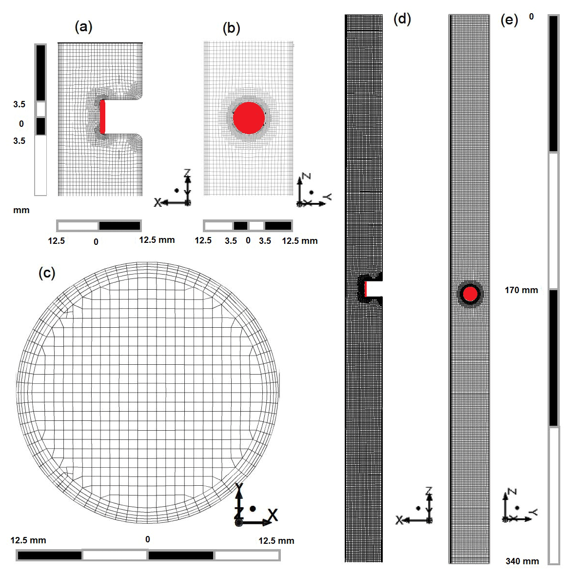
Figure 8 Cryogenic frost point hygrometer (CFH) intake tube mesh and geometry. The coordinate origin is located at the top centre of the intake tube. (a, b) Detailed views of the mirror holder on the y = 0 and x = 0 planes. (c) Intake tube cross section. (d, e) Intake tube on the y = 0 and x = 0 planes. Images used courtesy of ANSYS, Inc.

The mesh is shown in Fig. 8. As a mesh assembly method we used “cut cell”, which provides cuboid-shaped elements aligned in the flow direction. Simulations had to cover conditions from the lower troposphere, where the liquid- and mixed-phase clouds occurred, to the lower stratosphere where the sublimation of ice from the intake walls took place. This required coping with Reynolds numbers (Re) of the order of 5000 in the cloud (i.e. turbulent flow inside the tube) to 300 in the stratosphere (i.e. laminar flow) accompanied by a transition around Re ∼ 2300 from turbulent to laminar regimes:

$$\begin{array}{}\text{(3)}& \mathit{Re}={\displaystyle \frac{\mathit{\rho }\mathit{v}L}{\mathit{\mu }}},\end{array}$$

where ρ is the fluid's density in kg m⁻³ (here of air), v is the fluid's velocity in m s⁻¹ (relative to the intake tube), L is a characteristic linear dimension in m (here the tube diameter), and μ is the fluid's dynamic viscosity in kg m⁻¹ s⁻¹. We were especially interested in the near-wall effects, since the sublimation and the collision efficiency were evaluated near the wall. To enhance the mesh description near the wall, the first layer thickness is 0.2 mm. The subsequent layers grow in thickness at a rate of 1.2 for a total of five layers before the scheme changes from radial to Cartesian coordinates with a grid spacing of 1.5 mm.

4.2 FLUENT computational fluid dynamics software

We used a 3D steady-state pressure-based solver. As recommended for wall-affected flow with small Reynolds numbers, where turbulent resolution near the wall is important, we used an SST (shear stress transport) k-ω model (CFDWiki, 2011; ANSYS, 2012). The fluid material, air, was treated as a three-substance mixture of N₂, O₂ and H₂O. We specified how FLUENT computes the material properties, namely calculating density (ρ) using an incompressible ideal gas law:

$$\begin{array}{}\text{(4)}& \mathit{\rho }={\displaystyle \frac{p_{\mathrm{op}}}{RT{\sum }_i\frac{m_i}{M_i}}},\end{array}$$

where p_op is the simulation-defined operating pressure in Pa, R is the ideal gas constant, T is the absolute temperature, and m_i and M_i are the mass fraction and molar mass of species i, respectively. Heat capacity (c_p) was calculated using a FLUENT-defined mixing law:

$$\begin{array}{}\text{(5)}& c_p=\sum _i{m}_i{c}_{p,i}.\end{array}$$

In the dilute approximation scheme, the mass diffusion flux of a chemical species in a mixture was calculated according to Fick's law:

$$\begin{array}{}\text{(6)}& J_i=\mathit{\rho }{D}_i{\displaystyle \frac{\partial m_i}{\partial x}},\end{array}$$

where D_i is the diffusion coefficient of species i in the mixture. This relation is strictly valid when the mixture composition stays approximately constant and the mass fraction m_i of a species is much smaller than 1. The amount of water expected in the simulations was less than 1000 ppmv; therefore, the dilute approximation for the diffusion of water vapour in air, i = H₂O, was an accurate description.

The temperature and pressure dependencies of the diffusion coefficient of H₂O in air were given by Pruppacher and Klett (1997)

$$\begin{array}{}\text{(7)}& D=\mathrm{0.211}{\displaystyle \frac{{\mathrm{cm}}^{\mathrm{2}}}{\mathrm{s}}}{\left({\displaystyle \frac{T}{T_{\mathrm{0}}}}\right)}^{\mathrm{1.96}}\left({\displaystyle \frac{p_{\mathrm{0}}}{p}}\right),\end{array}$$

where T₀ = 273.15 K and p₀ = 1013.25 hPa.

For the viscosity and thermal conductivity, no mixture laws were considered. The values of viscosity and thermal conductivity were derived from a linear fit to air viscosity and thermal conductivity of dry air (EngineeringToolbox, 2005). Air viscosity was ${\mathit{\mu }}_{\mathrm{a}}\left(T\right)=\left(\mathrm{0.0545}\times (T/K)+\mathrm{2.203}\right)\times {\mathrm{10}}^{-\mathrm{6}}$ in kg m⁻¹ s⁻¹ and air thermal conductivity was $k_{\mathrm{a}}=\mathrm{8.06}\times {\mathrm{10}}^{{}^{-\mathrm{5}}}\times (T/K)+\mathrm{2.02}\times {\mathrm{10}}^{{}^{-\mathrm{3}}}$ in W m⁻¹ K⁻¹, both for T∈ (193, 300 K). According to kinetic gas theory, both properties are only weakly pressure-dependent (neglected here).

Velocity-inlet and pressure-outlet boundary conditions were defined for the intake tube. For the velocity-inlet boundary conditions, it was possible to define the velocity magnitude and direction, turbulence intensity, and temperature.

4.2.1 Velocity and flow profiles

Figure 9a–b show two examples of velocity profiles computed by FLUENT for two pairs of pressures and temperatures as they occurred in NT011, p = 310 hPa and T = −20 ^∘C and p = 33 hPa and T = −58.7 ^∘C. The two examples were done for the same inlet velocity of 5 m s⁻¹. In the lower-pressure case, the Reynolds number was low and the flow was laminar. In the higher-pressure case the Reynolds number was higher than 2300 and the flow was turbulent. As expected for the flow in a cylindrical tube, the flow velocity decreased towards the tube walls, became zero at the wall and in return accelerated at the centre of the tube, thus conserving mass flux. For our simulations, we took the balloon ascent velocity as the velocity of the flow entering the intake tube at the top plane.

Figure 9 (a, b) FLUENT simulation results for airflow velocity (centre cut through mirror holder). (a) p = 310 hPa and T = −20 ^∘C and (b) p = 33 hPa and T = −58.7 ^∘C simulations with inlet velocity 5 m s⁻¹ normal to the inlet plane. (c) Collision efficiency analysis based on FLUENT simulation results for particle tracks of hydrometeors with radii between 10 and 500 µm (colour-coding). The figure shows the top 7 cm of the intake tube. Flow simulations are for the mixed-phase cloud of flight NT011, p = 310 hPa and T = −20 ^∘C. Inlet velocity is ${\mathit{w}}_{\left|\right|}$ = 7.5 m s⁻¹ parallel to the tube (largely due to the balloon's ascent velocity) and v_⊥ = 6 m s⁻¹ perpendicular to the tube wall (largely due to the swinging motion of the payload), which results in an impact angle β of about 39^∘. Images used courtesy of ANSYS, Inc.

The mirror holder slowed the flow upstream, created a recirculation region downstream, and accelerated the flow in front of the mirror. The flow accelerated up to 150 % of the fully developed flow velocity in the tube centre. In the troposphere, the medium was denser and the flow was in the turbulent regime. Turbulent flows develop faster into a fully developed regime; see Fig. 9a–b.

4.2.2 Discrete-phase model

We used FLUENT's discrete-phase module to compute the collision efficiency for water droplets entering the tube together with the air at some impact angle. The droplets were accelerated in the same direction as the airflow when they entered the tube and either managed to avoid a collision with the wall or hit it at some distance down the tube. We injected one particle through each of the cells at the top inlet plane and repeated this procedure for droplets of different sizes. For each of the mixed-phase cloud simulations, we defined the droplet diameter, impact angle β and velocity magnitude. At the top of the tube, the impact angles and velocities of the droplets were assumed to be identical to the airflow.

The simulations in Fig. 9c were run with NT011 cloud conditions, p = 310 hPa and T = −20 ^∘C. The velocity at the intake tube inlet surface was 7.5 m s⁻¹ in the parallel component (z direction) and 6 m s⁻¹ in the perpendicular component (x direction), which corresponded to an impact angle of about 39^∘. For clarity, Fig. 9c displays only one every sixth droplet trajectory. Only the first 7 cm of the intake tube are shown. As expected, the airflow affected different size droplets differently. Smaller droplets had less inertia and hence tended to stay within the airflow, avoiding collisions with the tube's wall, while bigger droplets (with higher inertia) could not follow the streamlines and collided with the walls. Most 10 µm radius droplets avoided collision, while only the droplets entering very close to the intake tube wall collided. The bigger droplets to some extent also re-adjusted with the flow, but many of them collided within the first 5 cm of the intake tube. Above 70 µm droplet radius there was no dependence of the total collision efficiency on droplet size due to their large inertia.

In order to calculate the build-up of ice by impaction and considering how the injection of liquid droplets was set up in FLUENT, with one droplet per cell in the top inlet plane, we had to account for the mesh cell surface density. As discussed above, the cell surface density was higher closer to the intake tube wall (see Fig. 8c). Therefore, we normalized all collision efficiency results to the top inlet plane cell surface density, removing the effect of the mesh density from the results. The collision efficiency results are provided in Figs. 11, S6, S14 and S15 for the different mixed-phase clouds considered.

4.2.3 Species transport

The two key aspects controlling the level of contamination are the temperature of the ice layer and intake tube and the length of the ice layer inside the intake tube. Warmer ice provides the incoming air with a higher content of water vapour than colder ice. Simulations with longer ice layers inside the intake tube present more severe contamination than simulations with shorter ice layers at the same air temperature.

We simulated the sublimation of ice into the gas flow by assuming the cells adjacent to the icy wall to be saturated with respect to ice (using the vapour pressure parameterization of Murphy and Koop, 2005). The tube was assumed to have the same temperature as the airflow (Vömel et al., 2007b). In the UTLS, the intake tube might be slightly warmer than ambient air due to radiative heating. However, we do not expect this difference to be bigger than a few tenths of a Kelvin (Philipona et al., 2013). The tube wall was divided in ring sections and each was controlled separately to create the effect of a longer or shorter ice layer inside the intake tube. FLUENT calculated the distribution of the water vapour through the intake tube with a combination of molecular diffusivity (Eq. 6) and eddy diffusivity.

Figure 10 displays colour-coded vapour mixing ratios for different assumptions on the size of ice-covered area in the upstream part of the tube. For these simulations we took stratospheric conditions with p =  33 hPa and T = −58.7 ^∘C. The flow speed was 4.7 m s⁻¹ normal to the inlet surface. For cases (a)–(d), the ice covered the full inner circumference of the tube and extended for 15 and 5 cm from the rim into the flow direction and for 1 cm and 1.5 mm from 4 cm from the rim into the flow direction, respectively. Panel (e) shows the effect of a circumferentially asymmetric patch, which covered one eight of the intake circumferences and extended for 1 cm (between 4 and 5 cm), as an example of a case where a single larger hydrometeor hit the tube or of an ice layer, which sublimated inhomogeneously. As a general relationship, a larger icy coverage extent resulted in higher contamination. However, the relation between ice coverage in the tube and contamination was not linear. In dry stratospheric air (S_ice ∼ 0.01), a 15 cm long ice cover achieved S_ice ∼ 0.6 on average in the tube's volume, while a 1 cm long ice cover still achieved S_ice ∼ 0.15 on average in the tube's volume.

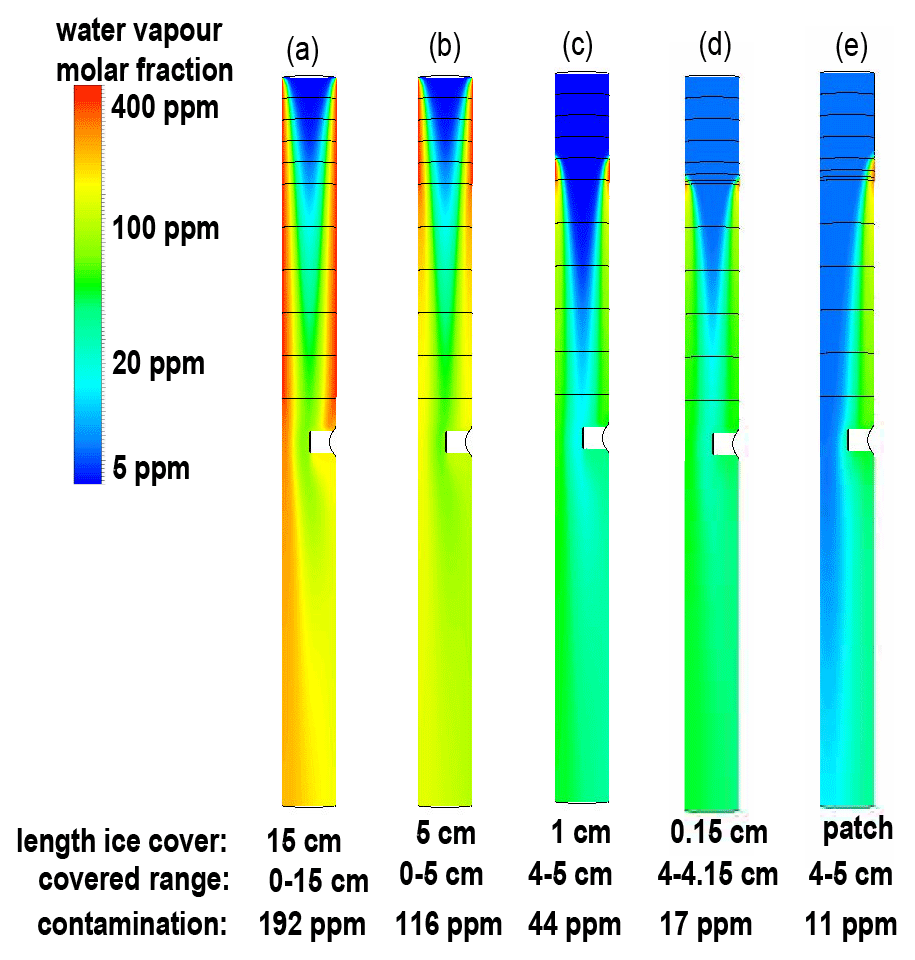
Figure 10 FLUENT simulation results for ice sublimation in the stratosphere with colour-coded H₂O mixing ratios for p = 33 hPa and T = −58.7 ^∘C with different ice coverage of the intake tube: (a) 15 cm with $\langle {\mathit{\chi }}_{{\mathrm{H}}_{\mathrm{2}}\mathrm{O}}{\rangle }_{\mathrm{Vol}}$ = 192 ppmv averaged over the tube volume, (b) 5 cm with $\langle {\mathit{\chi }}_{{\mathrm{H}}_{\mathrm{2}}\mathrm{O}}{\rangle }_{\mathrm{Vol}}$ = 116 ppmv, (c) 1 cm with $\langle {\mathit{\chi }}_{{\mathrm{H}}_{\mathrm{2}}\mathrm{O}}{\rangle }_{\mathrm{Vol}}$ = 44 ppmv, (d) 0.15 cm with $\langle {\mathit{\chi }}_{{\mathrm{H}}_{\mathrm{2}}\mathrm{O}}{\rangle }_{\mathrm{Vol}}$ = 17 ppmv and (e) circumferentially asymmetric patch of 1∕8 intake tube circumference and 1 cm length with $\langle {\mathit{\chi }}_{{\mathrm{H}}_{\mathrm{2}}\mathrm{O}}{\rangle }_{\mathrm{Vol}}$ = 11 ppmv. The triangular brackets indicate mixing ratios that have been averaged over the full tube volume. Images used courtesy of ANSYS, Inc.

Figure 10 shows how contamination diffuses from the tube walls towards the centre of the tube. Over the length of the tube (34 cm) the contamination homogenized, whereas at the position of the mirror, 17 cm from the top of the tube, the H₂O flow was not yet homogeneous. This internal gradient resulted from the residence time τ ∼ 0.07 s of the air inside the tube (34 cm long and moving with 4.7 m s⁻¹), so that a molecular diffusivity 4.0 cm² s⁻¹ (see Eq. 7) allowed the H₂O molecules to travel on average only a distance (τD)^1∕2 ∼ 0.5 cm towards the tube centre. The resulting boundary layer was clearly visible in the upper parts of the tubes shown in Fig. 10. Any further diffusion can be attributed to eddy diffusivity, which the turbulence scheme of FLUENT was designed to properly determine. In this range of the stratosphere, eddy diffusivity was about 5000 cm² s⁻¹ (Massie and Hunten, 1981); however, this value applies to the large-scale stratospheric dimensions, not to the small dimensions inside the tube. The effective diffusivity was somewhere between the molecular and the free stratospheric value, as calculated by FLUENT.

In this study, we preferred mixing ratios averaged over the entire volume of the intake tube instead of area-averaged water vapour mixing ratios at the mirror surface. The latter were 60 % to 50 % smaller than the former for the same simulation. We believe that the entire flow of air through the intake tube influences the frost point temperature, and not just the air flowing right next to the mirror.

We investigated the influence of an inlet airflow not parallel to the tube. Although a different impact angle than 0^∘ disturbed the flow in the first centimetres of the tube, the flow recovered quickly. The uptake of water vapour from the icy wall into the airflow in these first few centimetres became radially asymmetric. However, over the length of the tube it homogenized, and on average we obtained the same level of contamination independent of the impact angle. Therefore, for the stratospheric and upper tropospheric ice sublimation simulations in Sect. 5.2 and 5.3, respectively, we compared observed contaminated H₂O mixing ratios to simulated volume-averaged H₂O mixing ratios ($\langle {\mathit{\chi }}_{{\mathrm{H}}_{\mathrm{2}}\mathrm{O}}{\rangle }_{\mathrm{Vol}}$) and only considered flow parallel to the tube. Evidently, this was in contrast to the hydrometeor simulations, for which even small impact angles made a big difference.

5 Results

5.1 Hydrometeors freezing efficiency derived from impact angles

To estimate the collision efficiency of supercooled droplets during the cloud passage in flight NT011, we performed 10 FLUENT simulations as described in Sect. 4.2.2, using ${\mathit{w}}_{\left|\right|}$ = 7.5 m s⁻¹ for the velocity component parallel to the tube (see Figs. 6b and 7b). For each of the 10 FLUENT simulations we took a different perpendicular velocity v_⊥ to the tube walls as shown in Fig. 7a for steps of 1, 2, 3, … to 10 m s⁻¹.

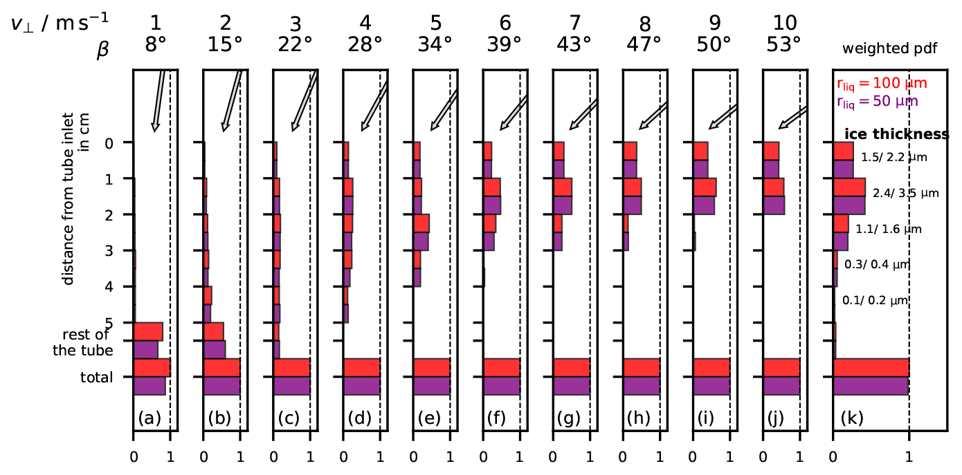
Figure 11 Collision/freezing efficiency of hydrometeors in the intake tube for the flight NT011 mixed-phase cloud with average vertical inlet velocity ${\mathit{w}}_{\left|\right|}$ = 7.5 m s⁻¹. r_liq = 100 µm (red); r_liq = 50 µm (purple). (a–j) Freezing efficiency for various velocities (v_⊥) perpendicular to the tube walls and impact angles β: (a) 1 m s⁻¹, 8^∘; (b) 2 m s⁻¹, 15^∘; (c) 3 m s⁻¹, 22^∘; (d) 4 m s⁻¹, 28^∘; (e) 5 m s⁻¹, 34^∘; (f) 6 m s⁻¹, 39^∘; (g) 7 m s⁻¹, 43^∘; (h) 8 m s⁻¹, 47^∘; (i) 9 m s⁻¹, 50^∘; (j) 10 m s⁻¹, 53^∘. The “rest of the tube” takes account of all collisions occurring deeper than 5 cm inside the tube, including the mirror holder. (k) Sum of the efficiencies from panels (a)–(j) weighted by the pdf of v_⊥ in Fig. 7a; behind each bar the thickness of the resulting ice layer is noted assuming a homogeneous ice cover inside the intake tube for the lower (left number) and upper (right number) LWC estimates for the cloud in NT011.

Figure 11 displays the computed collision efficiencies for perpendicular velocities (v_⊥) increasing from (a) to (j). The panels also list the corresponding impact angle (β). For each v_⊥, we considered droplet sizes of 100 and 50 µm radius. In each panel, the first 5 horizontal bars represent the first 5 cm of the tube, the 6th bar represents the rest of the tube (including the mirror holder) and the 7th bar is the sum of all the above, representing the probability of the droplet hitting the tube at all. Differences to 100 % represent droplet percentage that escapes the intake tube. Figure 11k shows the collision efficiencies weighted sum by the occurrence probability (pdf) of each v_⊥ as calculated for the NT011 cloud and shown in Fig. 7a.

For the droplet sizes and impact angles considered, 100 % of the 100 µm radius droplets and 96 % of the 50  µm radius droplets collided with the intake tube wall and more than 90 % of these collided within the first 4 cm. Figure 11k also lists the calculated thicknesses of the ice layer in the first 5 cm of the intake tube after passing through the cloud, assuming an even coverage of the intake tube inner surface and taking into consideration the simulated collision efficiencies and the upper and lower estimate of LWC that we discussed in Sect. 2.4. The first value listed for each horizontal bar in Fig. 11k refers to the lower LWC estimate and the second to the upper LWC estimate.

Figure 11 shows that the combination of high impact angles and big droplet sizes caused an ice layer to accumulate at the top of the intake tube, in the first 5 cm. Smaller impact angles, up to 15^∘ caused a more even coverage over the entire length of the intake tube (but occurred much less frequently; see Fig. 7c). As the layer remained quite thin (in the range of 1 to 4 µm), representing less than 1 ‰ of the intake tube radius, the ice layer did not affect the inlet flow. However, it had a detrimental influence on the water vapour measurement in the stratosphere.

Freezing efficiencies were also simulated for the mixed-phase clouds in flights NT007 and NT029 (Figs. S6, S14 and S15). One of the clouds encountered during flight NT007 (Fig. S10a–b) was warmer, allowing also smaller droplets to exist, which we considered in Fig. S14. The total freezing efficiency of the 10 µm radius droplets in the entire tube was smaller than 50 %. The collisions happened mainly in the first 2 cm of the intake tube and below the mirror holder.

5.2 Contaminated water vapour measurements in the stratosphere

5.2.1 Sublimation and sublimated water estimation

For the simulations of sublimation of ice in the intake tube, we used FLUENT in the configuration described in Sect. 4.2.3. We defined three scenarios of ice coverage of the intake tube as shown in Fig. 10a–c: coatings of 15 or 5 cm length starting at the rim of the intake tube and 1 cm coating starting 4 cm into the intake tube. We ran simulations approximately every km in the stratosphere driven by measurements of temperature, pressure, ascent velocity, and background water vapour mixing ratio averaged over 1 km intervals. In Fig. 12, we show stratospheric measurements during flight NT011 and the FLUENT simulation results. The values used as input in the simulations are shown in the stratospheric part of Table 2 as well as the simulation results. Figure 12a displays the air temperature, the average Naintial 2016 summer campaign air temperature and the ascent velocity parallel to the intake tube (${\mathit{w}}_{\left|\right|}$). Due to high variability in the ascent velocity, we calculated the standard deviation for each ascent-velocity-averaged point, shown in the graph as grey dots and error bars, and performed FLUENT simulations to investigate the influence of the ascent velocity variability. We concluded that ±2 m s⁻¹ had no significant impact on the simulated volume-averaged water vapour mixing ratio in the intake tube.

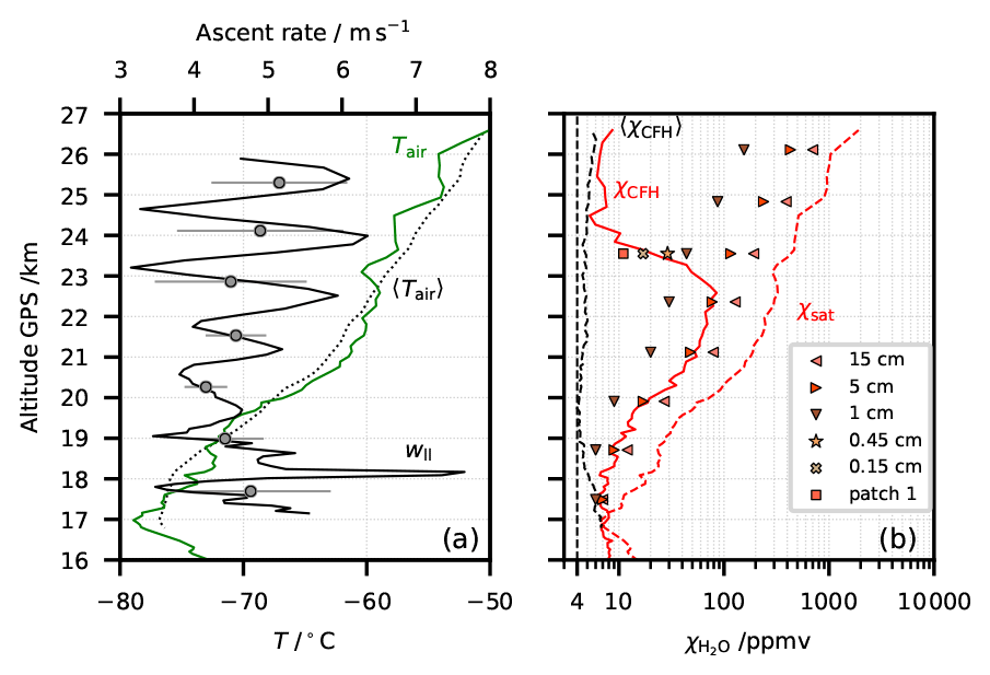
Figure 12 Flight NT011 and FLUENT simulation results for sublimation of ice in the intake tube in the stratosphere. (a) Green line: measured air temperature T_air; dotted black line: average air temperature for the 2016 Nainital summer campaign; solid black line: ascent velocity; circles: 1 km interval-averaged ascent velocity; horizontal grey lines: standard deviation. (b) Solid red line: H₂O mixing ratio measured by the CFH during NT011 (χ_CFH); dashed black line: average H₂O mixing ratio of the soundings during the 2016 Nainital summer campaign (〈χ_CFH〉) (excluding the contaminated profiles); dashed red line: saturation H₂O mixing ratio (χ_sat); other symbols: FLUENT simulation results for the tube average mixing ratios $\langle {\mathit{\chi }}_{{\mathrm{H}}_{\mathrm{2}}\mathrm{O}}{\rangle }_{\mathrm{Vol}}$ in tubes with different ice-coating depths d coating the full circumference: ◂ d = 15 cm; ▸ d = 5 cm; ▾ d = 1 cm; ⋆ d = 0.45 cm; x d = 0.15 cm; coating only 1∕8 intake tube circumference (patch): ▪ d = 1 cm.

Table 2 FLUENT stratospheric and upper tropospheric simulation input data and results for flight NT011.

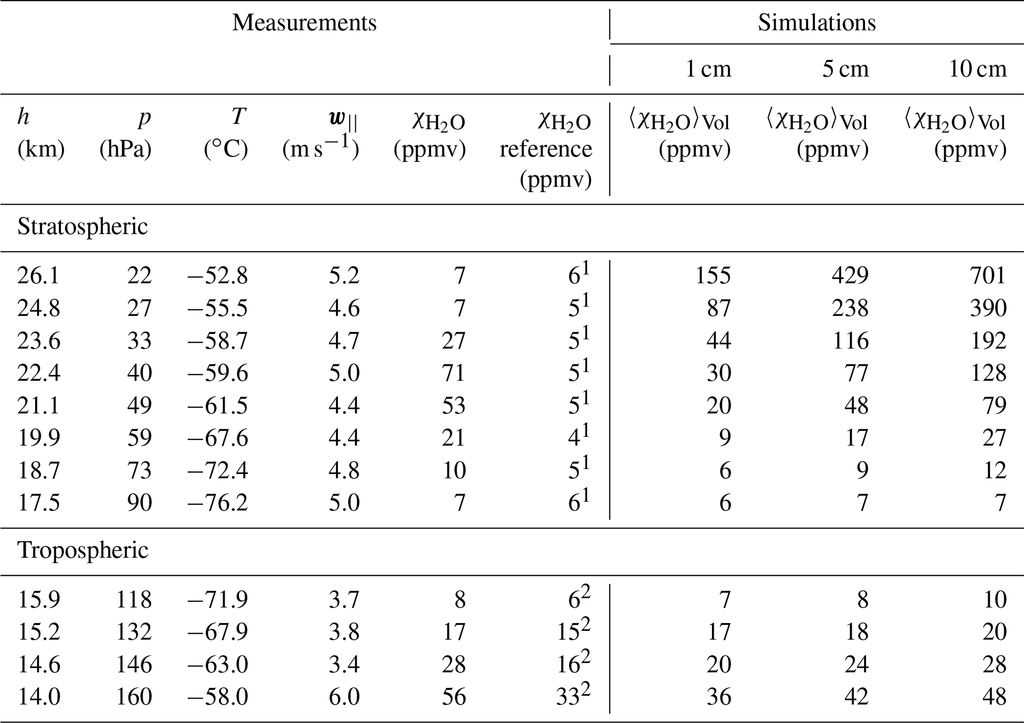
¹ 〈χ_CFH〉. ² χ_RS41.

In Fig. 12b, we show ${\mathit{\chi }}_{{\mathrm{H}}_{\mathrm{2}}\mathrm{O}}$ from the CFH (χ_CFH) and the average ${\mathit{\chi }}_{{\mathrm{H}}_{\mathrm{2}}\mathrm{O}}$ for the Nainital 2016 summer campaign (〈χ_CFH〉). We also show the saturation ${\mathit{\chi }}_{{\mathrm{H}}_{\mathrm{2}}\mathrm{O}}$ for flight NT011 calculated from the air temperature (χ_sat). The $\langle {\mathit{\chi }}_{{\mathrm{H}}_{\mathrm{2}}\mathrm{O}}{\rangle }_{\mathrm{Vol}}$ for the 15, 5 and 1 cm intake tube ice coverage are shown as different coloured triangles. $\langle {\mathit{\chi }}_{{\mathrm{H}}_{\mathrm{2}}\mathrm{O}}{\rangle }_{\mathrm{Vol}}$ for other ice coverage configurations, such as thinner rings and radially asymmetric patches, are shown at higher altitude as the measurement recovers from contamination.

From the comparison of the simulation results for ${\mathit{\chi }}_{{\mathrm{H}}_{\mathrm{2}}\mathrm{O}}$ in Fig. 12b, we concluded that the simulations with 5 cm ice coverage of the intake tube yielded the best description of the observations. This result was consistent with the collision efficiency results of Sect. 5.1. When the observed ${\mathit{\chi }}_{{\mathrm{H}}_{\mathrm{2}}\mathrm{O}}$ decreased, above 22 km altitude, the 5 cm simulation started to overestimate ${\mathit{\chi }}_{{\mathrm{H}}_{\mathrm{2}}\mathrm{O}}$. As the ice coverage decreased, the inlet airflow was exposed to a smaller ice surface and was less hydrated, until no ice surface was left and the instrument observed ambient ${\mathit{\chi }}_{{\mathrm{H}}_{\mathrm{2}}\mathrm{O}}$. The transition from 5 cm ice wall coverage was very fast. At 22 km altitude, the 5 cm simulation still matched the observation, while 1 km higher at 23 km altitude, we were able to match the observation to the 0.45 cm simulation. At 25 km altitude, we considered the measurement to be recovered. Figures S7 and S16 show similar results for the stratosphere of flights NT029 and NT007.

Considering the water vapour to be well mixed within the intake tube, knowing the pressure, temperature and the intake tube volume, and having a reference water vapour measurement, we could estimate the total ice sublimated in the stratosphere,

$$\begin{array}{}\text{(8a)}& {\displaystyle }\sum _i^N{\displaystyle \frac{p_{\mathrm{air}i}\mathrm{100}{V}_{\mathrm{tube}}}{R{T}_{\mathrm{air}i}}}\left({\mathit{\chi }}_{\mathrm{CFH}i}-{\mathit{\chi }}_{\mathrm{ref}i}\right),\text{(8b)}& {\displaystyle }N={\displaystyle \frac{h_{\mathrm{burst}}-h_{\mathrm{CPT}}}{\mathrm{100}{l}_{\mathrm{tube}}}}.\end{array}$$

We did the integration in intervals of 100 intake tube volumes between the CPT and balloon burst, because of the measurement resolution. Since the contamination disappeared before balloon burst, the total ice sublimated in the stratosphere was the total water frozen in the intake tube during the traverse through the mixed-phase cloud, depending on the conditions above the mixed-phase cloud in the troposphere.

Table 3 lists results for the stratospheric integration of water vapour for NT007, NT011 and NT029. A total of 4.35 mg of ice sublimated from the intake tube in the stratosphere in flight NT011 (derived from the difference between χ_CFH and 〈χ_CFH〉 in Fig. 12b; see Formula 8a). We considered this the lower estimate of water that froze in the intake tube during the ascent through the mixed-phase cloud, because a small part of the ice might have already sublimated between the mixed-phase cloud and the tropopause. The cloud extent was 750 m and the estimated collision and freezing efficiency of the hydrometeors in the cloud was 100 %, so the lower estimate of LWC in the cloud was 0.011 g m⁻³. This is very little LWC for a mixed-phase cloud, so we concluded that the mixed-phase was almost completely glaciated. We used this value as the lower estimate for LWC for the cloud simulation in Sect. 2.4. During the two other flights, more ice sublimated in the stratosphere.

Table 3 Integrated water vapour in the stratosphere and upper troposphere for flights NT007, NT011 and NT029.

5.2.2 Ice-layer evolution

As we saw from the collision efficiency results in Fig. 11k, the thickness of the ice coverage inside the tube was not uniform in the flow direction. Subsequently we show how this non-uniformity influences the sublimation and the lifetime of the ice coverage in the intake tube. For this, we computed the potential of ice at a certain position downstream in the tube to hydrate the passing air, thereby lowering the air subsaturation and, hence, slowing the sublimation of the ice further downstream. We ran FLUENT sublimation simulations with different ice coverage configurations of the intake tube for three altitudes (p = 15 hPa and T = −51.4 ^∘C; p = 25 hPa and T = −53.6 ^∘C; p = 39 hPa and T = −59.2 ^∘C). The results are listed in Table 4.

Table 4 Results for ice-layer evolution in the stratosphere due to sublimation. The “isolated” simulations refer to isolated 1 cm long rings in the flow direction covering the entire inner circumference of the intake tube. These 1 cm long rings start at different distances from the rim of the intake tube down to 4 cm. Results are given as an extra H₂O mixing ratio from the reference, which was ${\mathit{\chi }}_{{\mathrm{H}}_{\mathrm{2}}\mathrm{O}}$ ∼ 4 ppmv. The “in-group” simulations consider ice coverages of different lengths, all starting at the rim of the intake tube. For these simulations, extra ${\mathit{\chi }}_{{\mathrm{H}}_{\mathrm{2}}\mathrm{O}}$ is calculated as differences from subsequent simulations.

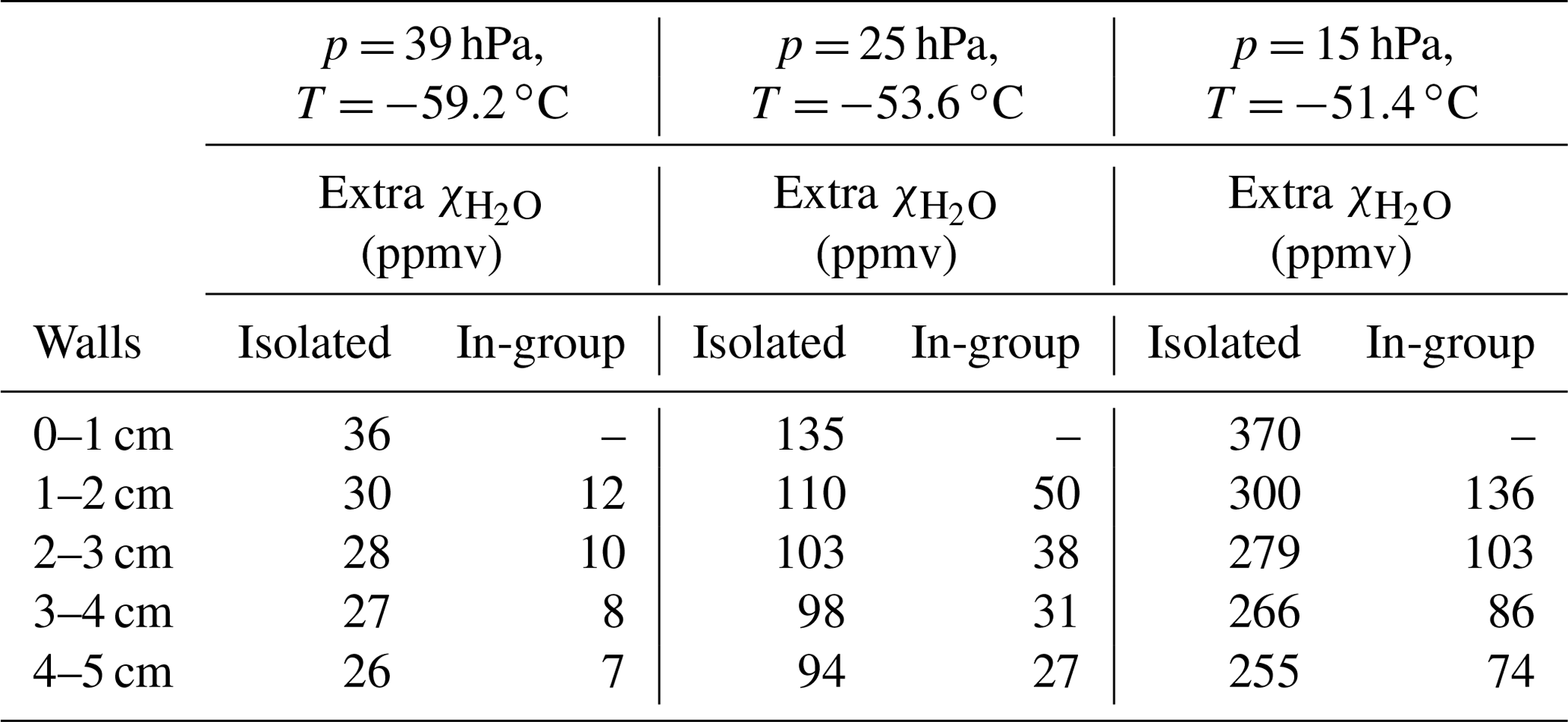
For the simulations named “isolated” in Table 4, we considered isolated 1 cm-long rings in the flow direction covering the entire inner circumference of the intake tube. These 1 cm-long rings started at different distances from the rim of the intake tube down to 4 cm. With these simulations, we could compare the potential of an isolated ice layer to hydrate passing stratospheric dry air at different distances from the rim of the intake tube. Results of these simulations are given as extra H₂O mixing ratio from the reference, which was ${\mathit{\chi }}_{{\mathrm{H}}_{\mathrm{2}}\mathrm{O}}$ ∼ 4 ppmv. The “in-group” type of simulations considered ice coverages of different length all starting at the rim of the intake tube. With these simulations we could estimate the added contribution of an ice ring at a certain distance from the rim, once the passing air has already experienced a certain level of contamination caused by the ice on the tube wall above. For these simulations, extra ${\mathit{\chi }}_{{\mathrm{H}}_{\mathrm{2}}\mathrm{O}}$ was calculated as differences from subsequent simulations. From 5 cm from the rim of the intake tube, the isolated rings become 2 cm long down to 15 cm from the intake tube rim and the ice layers extending from the intake tube rim increase length in 2 cm steps also down to 15 cm from the rim of the intake tube. The results for these simulations are shown in Table 5 but only for one of the pressure and temperature pairs used in the simulations shown in Table 4. This analysis confirms that the first centimetre of the intake tube was the most efficient at hydrating the passing air compared to ice downstream. When the passing air had already been in contact with an icy surface, the hydration efficiency of the subsequent ice layers reduced strongly.

Table 5 Results for ice-layer evolution in the stratosphere due to sublimation–continuation. From 5 cm from the rim of the intake tube, the isolated rings become 2 cm long down to 15 cm from the intake tube rim and the ice layers extending from the intake tube rim increase in length in 2 cm steps also down to 15 cm from the rim of the intake tube. Only one of the pressure and temperature pairs used in the simulations shown in Table 4 is presented.

^∗ Note that these walls are 2 cm long instead of 1 cm.

The lower layers, more than 5 cm inside the tube, had the smallest contribution to the air hydration, but they sublimated first after passing the cloud because the ice deposition from the hydrometeor collisions was also small (Fig. 11k). Of the top layers, hit most frequently by the impacting hydrometers within the mixed-phase cloud, we expected the first layer to be the first to sublimate. After the first centimetre of the intake tube became ice-free, the strongest contamination arose from the next layer downstream. The layer between 1 and 2 cm was also the thickest layer (Fig. 11k); i.e. it had an extended lifetime. The layers below were thinner but they also contributed to the hydration of the flow. Independent of which of the layers between 1 and 4 cm from the rim of the intake tube sublimated next, once isolated, any 1 cm long ring in this region contributed very similar amounts of water vapour to dry incoming stratospheric air. This suggested that the contamination stayed significant as long as some ice was in the tube, but thereafter disappeared readily. This was confirmed by the ice patch and thinner layer (0.45 or 0.15 cm) simulations. Figure 12b shows these results at 23.5 km altitude.

In summary, the ice deeper inside the tube sublimated less quickly, but it nevertheless disappeared first, because only a thin layer of ice was deposited there when traversing the cloud. Thereafter, the ice layer sublimated fastest from the top of the intake tube, because hydration was more efficient when the air is at stratospheric dryness. Figure 12b reveals that the FLUENT simulations together with reasonable assumptions about the initial contamination in the mixed-phase cloud can achieve a good agreement with the measurements.

5.3 Considerations regarding the upper troposphere

The contamination in the stratosphere was a remarkable feature and was relatively easy to spot since the expected water vapour mixing ratio values were in a well-defined range 2–6 ppmv. Sublimation may also occur in the upper troposphere after passing through mixed-phase clouds, although it might be harder to identify. For the stratospheric contamination we had a readily available reference, namely the mean of the campaign measurements excluding the contaminated flights. Water vapour in the stratosphere has very limited day-to-day variability, whereas tropospheric water vapour is extremely variable. We investigated whether the relative humidity measurement by the RS41 radiosonde could serve as a reference. Brunamonti et al. (2019) found the RS41 to have, on average, a dry bias in comparison with the CFH in the upper troposphere during StratoClim. However, in a flight-by-flight comparison, when the CFH was contaminated, it was not clear whether the RS41 had a dry bias or the CFH measured a too high humidity. As a conservative assumption, we assumed the RS41 water vapour measurement to be correct, and we used it as a reference for the analysis of the CFH contamination in the upper troposphere.

Figure 13 Flight NT011 and FLUENT simulation results for sublimation in the upper troposphere. (a) Green: air temperature; black: ascent velocity. (b) Red: H₂O mixing ratio by the CFH; orange: H₂O mixing ratio by the RS41; dashed red: saturation H₂O mixing ratio for the air temperature; symbols: FLUENT simulation results for the tube average mixing ratios $\langle {\mathit{\chi }}_{{\mathrm{H}}_{\mathrm{2}}\mathrm{O}}{\rangle }_{\mathrm{Vol}}$ in tubes with different ice-coating depths d (full circumference): ◂ d = 15 cm; ▸ d = 5 cm; ▾ d = 1 cm; (c) light blue: saturation over water (S_liq,RS41) by the RS41; pink: saturation over water (S_liq,f) from the CFH considering the deposit on the mirror to be frost; blue: ice saturation (S_ice) from the CFH; grey: 940 nm backscatter ratio from the COBALD. Horizontal dashed lines limit the integration interval used for estimating the sublimated ice in the upper troposphere.

Figure 2 shows that the profile of NT011 between the top of the lower cloud and the cirrus cloud at the tropopause was subsaturated. In Fig. 13, we provide a detailed view of this region of the flight (13–17.5 km altitude). Figure 13a–b are analogous to Fig. 12a–b with the exception that in panel (b) we do not show 〈χ_CFH〉, but χ_RS41 of NT011. Figure 13c shows the same variables as Fig. 3b. The dry bias of the RS41 relative to the CFH is noticeable in the region between 13.5 and 17 km, right up to the CPT. At 14.0, 14.6 and 15.9 km altitude there was a significant difference between the CFH and the RS41 ${\mathit{\chi }}_{{\mathrm{H}}_{\mathrm{2}}\mathrm{O}}$ (see tropospheric part of Table 2). Observed S_liq was below 30 % and S_ice was below 70 %. The difference in water vapour mixing ratio for the two instruments was about 50 %–70 % which can not be accounted for by the estimated 10 % uncertainty of the CFH measurement (Vömel et al., 2007b), also not by the estimated 3 %–9 % dry bias of the RS41 relative to the CFH (Brunamonti et al., 2019), nor by a combination of both. At 15.2 km altitude, the observed ${\mathit{\chi }}_{{\mathrm{H}}_{\mathrm{2}}\mathrm{O}}$ for the RS41 was within the CFH uncertainty, and S_liq was 30 % and S_ice was 70 %.

To understand whether the proposed mechanism of sublimation from an ice layer at the top of the intake tube might explain the dry/wet bias observed, we ran FLUENT simulations at four selected altitudes (see symbols in Fig. 13b). Pressure, temperature, inlet velocity and background water vapour from the RS41 used for the FLUENT simulations are presented in the tropospheric part of Table 2, where the simulation results are again presented as $\langle {\mathit{\chi }}_{{\mathrm{H}}_{\mathrm{2}}\mathrm{O}}{\rangle }_{\mathrm{Vol}}$. In Fig. 13b, at 14 and 14.6 km altitude, the simulations for the 15 cm ice coverage of the intake tube could account for the extra water vapour measured by the CFH. The location at 15.2 km altitude showed the limit of the FLUENT simulations. The simulation considering 1 cm ice coverage matches the CFH observation and the other two ice coverages considered (5 and 15 cm) over-estimated the CFH observation. Although the observations did not show ice saturation, the dilute approximation used in the FLUENT simulation (see Sect. 4.2) is no longer valid for S_ice ≥ 70 %, and the simulations over-estimated how much ice sublimated into the airflow. The CFH observation at 15.9 km altitude could be due to the presence of a 5 cm ice layer at the top of the intake tube. The lower 10 cm of the ice-layer cloud have sublimated between the lower observation at 14.5 km height and the observation at 15.9 km.

In flight NT007 (Fig. S17) the RS41 measured lower water vapour mixing ratio than the CFH in the upper troposphere as expected. However, once S_ice approached 1 at 13.8 km altitude, the CFH measured less water vapour than the RS41. We suppose that the icy intake tube top was having the opposite effect in contaminating the CFH measurement. It was depleting the gas-phase water vapour and growing the ice coverage, reducing the supersaturation which in a clean intake tube case would have been observed.

To estimate an upper limit for the LWC in the mixed-phase cloud, we compared the total water vapour measured by the CFH and the RS41 using Formula (8a) in the interval between the top of the lower cloud and the cirrus cloud at the tropopause (from 13.5 to 17 km altitude). We concluded that the CFH measured at least 1.45 mg of water more than the RS41 in this interval. This was about one-third of the ice sublimating in the stratosphere and could be additional water that accumulated inside the intake tube as ice during the mixed-phase cloud and sublimated in the upper troposphere. Adding this ice to the ice sublimated in the stratosphere, gave a total of 5.8 mg of ice sublimated in flight NT011. Table 3 shows total integrated water vapour and integrated water vapour for the stratosphere and upper troposphere for flights NT007, NT011 and NT029. In flights NT029, there was a cirrus clouds in the upper troposphere, so the water vapour integration is done below and above the cirrus cloud. From the total integrated water vapour for the different flights, we calculated upper estimates of LWC for the cloud simulation in Sect. 2.4. These values are shown in Table 1 together with lower estimates of LWC.

5.4 Other types of contamination

Besides the intake tube, there may be other sources of contamination, such as the balloon envelope, the nylon cord, or the instrumental payload. Here, we differentiate the various contamination sources. We did two extra related studies with FLUENT. The principle of the implemented simulations was identical to what was described in Sect. 4.2.

5.4.1 Balloon envelope

We ran FLUENT simulations for typical tropospheric and stratospheric conditions shown in Table 6. We used a new mesh, for which the balloon radius changed with pressure. We considered an initial balloon size of 1 m radius at 800 hPa and 25 ^∘C, approximately corresponding to the launching conditions at Nainital (1820 m a.s.l.) during the summer season. As the payload ascends, the balloon radius increases; see Table 6. In the simulation, we placed the CFH package 55 m below the balloon centre and considered two different ascent velocities (4 and 7 m s⁻¹), and the entire surface of the balloon to be covered with an ice layer, implemented similarly to the ice-covered intake tube. The simulation domain extended 5 m from the balloon surface in every direction and 5 m below the CFH package; see Fig. 14.

Table 6 FLUENT input values (P, T and background ${\mathit{\chi }}_{{\mathrm{H}}_{\mathrm{2}}\mathrm{O}}$ for typical tropospheric and stratospheric conditions) for simulations of contamination stemming from the balloon envelope and resulting ${\mathit{\chi }}_{{\mathrm{H}}_{\mathrm{2}}\mathrm{O}}$ directly (d=0 m) and 5 to 10 m displaced from under the balloon (d=5–10 m), 55 m below the balloon–payload (CFH) location. The balloon radius changes with height. Two different balloon ascent velocities (w) were considered.

Figure 14 Contamination below a balloon: central cuts through a completely icy balloon and its wake showing the H₂O mixing ratio (a) at 50 hPa and (b) at 20 hPa; oscillations of the payload 55 m below the balloon measured by GPS during NT007 (c) from 20 to 22 km altitude (50 hPa level) and (d) from 28 to 31 km altitude (20 hPa level). Red circle: balloon cross sections at respective pressure levels. Images used courtesy of ANSYS, Inc.

In Fig. 14a–b, we see the water vapour mixing ratio colour coded for the balloon and payload ascending at 7 m s⁻¹ at the 50 and 20 hPa levels, respectively. At the 50 hPa level, the excess water vapour due to balloon contamination was still moderate. The water vapour mixing ratio observed 55 m below the balloon at the payload level was within the stratosphere natural variability (4–8 ppmv). At the 20 hPa level, the effect of contamination by the balloon was large. The enhanced water vapour mixing ratios in the wake of the balloon extended by 6 m in radius at the payload level and reached up to 100 ppmv. The contamination values directly below the balloon were upper limits of contamination. If we considered the payload oscillation at these altitudes, we would see that the CFH was consistently out of the balloon wake, where there was no contamination, in the case at 50 hPa (see Fig. 14c). At the 20 hPa level, the payload oscillation showed a nearly perfect circular movement around the balloon, with a displacement between 5 and 10 m (see Fig. 14d), where ${\mathit{\chi }}_{{\mathrm{H}}_{\mathrm{2}}\mathrm{O}}$ was less than 10 ppmv (see Fig. 14b). At 10 hPa, not shown, the balloon radius was larger and, consequently, so was the wake of the balloon. At this pressure level, the payload showed a similar displacement from under the balloon as observed in Fig. 14d. When the payload was 5 m displaced from under the balloon ${\mathit{\chi }}_{{\mathrm{H}}_{\mathrm{2}}\mathrm{O}}$ was approximately 40 ppmv, 10 m displaced from under the balloon ${\mathit{\chi }}_{{\mathrm{H}}_{\mathrm{2}}\mathrm{O}}$ was approximately 5 ppmv.

Figure 15 compares the expected magnitude of the contamination from the balloon envelope with the contaminated ${\mathit{\chi }}_{{\mathrm{H}}_{\mathrm{2}}\mathrm{O}}$ observations by the CFH in StratoClim 16/17. Figure 15 shows all the contaminated profiles which have been shown in Fig. 1, and the campaign season averages (〈χ_CFH〉_NT and 〈χ_CFH〉_DK) excluding the contaminated flights. The light red shaded region highlights expected ${\mathit{\chi }}_{{\mathrm{H}}_{\mathrm{2}}\mathrm{O}}$ if there was contamination from the balloon skin and the payload travelled directly below the balloon or within a 5 m radius centred 55 m below the balloon. The dark red region identifies ${\mathit{\chi }}_{{\mathrm{H}}_{\mathrm{2}}\mathrm{O}}$ for balloon contamination if the payload stayed outside this 5 m radius circular region centred 55 m directly below the balloon. The contaminated ${\mathit{\chi }}_{{\mathrm{H}}_{\mathrm{2}}\mathrm{O}}$ observed during StratoClim 16/17 were at least 1 order of magnitude higher than the balloon contamination. Hence, we can consider the balloon envelope as a minor contributor to the contamination.

Figure 15 Comparison of expected contamination from the balloon envelope with contaminated ${\mathit{\chi }}_{{\mathrm{H}}_{\mathrm{2}}\mathrm{O}}$ observations by the CFH in StratoClim 16/17. Black dots: all contaminated profiles of StratoClim 16/17 (see Fig. 1), black line: Nainital 2016 season average, grey line: Dhulikhel 2017 season average, light red region: expected contamination when the payload travels directly below the balloon or within a 5 m radius 55 m below the balloon, dark red region: expected balloon contamination if the payload stays outside the 5 m radius circular region 55 m directly below the balloon.

However, the balloon envelope could be the source of the contamination observed from 20 hPa onwards in all flights; see Fig. 1b of Brunamonti et al. (2018). The average profiles of water vapour mixing ratio for StratoClim 16/17 showed 6 to 20 ppmv ${\mathit{\chi }}_{{\mathrm{H}}_{\mathrm{2}}\mathrm{O}}$ between 20 and 10 hPa, which are too high compared to stratospheric water vapour mixing ratios. Note how above the 20 hPa level the dark red area in Fig. 15 overlaps the StratoClim campaign averages: 〈χ_CFH〉_NT and 〈χ_CFH〉_DK.

The difference in contamination 55 m below the balloon due to different ascent velocities was not significant, less than 10 % ${\mathit{\chi }}_{{\mathrm{H}}_{\mathrm{2}}\mathrm{O}}$. We also investigated the contamination observed 55 m below the balloon, when only half of the balloon surface was covered in ice. We found the contamination to be approximately half of that observed for the full coverage of the balloon skin. We also investigated balloon contamination in the upper troposphere. We ran a simulation for 200 hPa with background water vapour of 100 ppmv. At this level and temperature of −40 ^∘C, water vapour saturation is 600 ppmv. At the position of the payload, 55 m below the balloon, we could expect an extra 12 ppmv. The contamination was not negligible, but it was comparable to the instrumental uncertainty of the CFH (10 %) and it would also be detected by the capacitive humidity sensor on the RS41 radiosonde, hence it cannot be uniquely identified.

5.4.2 Instrument package

We examined possible contributions from the instrument housing, i.e. the Styrofoam package, to the observed contamination. To this end, we ran simulations for the atmospheric conditions summarized in Table 6 and used an instrument package geometry and mesh including intake and outlet tubes; see Fig. 16. The CFH package is rectangular (12 cm × 17 cm × 31 cm) and not symmetric, as the intake tube is not located at the centre of the package. It is centred along the shorter dimension (Fig. 16b) but asymmetrically positioned along the longer dimension (Fig. 16c). The simulation domain extended by 25 cm above the top of the intake tube, 30 to 35 cm beyond the CFH package sides, and by 150 cm below the outlet tube and allowed for a realistic development of the flow around and below the payload. Figure 16 displays only a reduced part of the domain. The simulation referred to 20 hPa atmospheric pressure with 7 m s⁻¹ ascent velocity, assuming the top surface of the CFH box to be ice-covered. Figure 16 shows the flow velocity field (panel a), the resulting distribution of H₂O mixing ratio from the two major viewing angles (panels b and c), and the mixing ratio for an hypothetical CFH with a shorter intake tube (panel d). The intake tube normally extends by 12 cm above the box, but in the experimental version in panel (d) only by 6 cm.

Figure 16 Contamination caused by an icy CFH box (Styrofoam) at 20 hPa assuming a balloon ascent velocity of 7 m s⁻¹. (a) Flow velocity around the CFH housing; (b–c) H₂O mixing ratio for two side views of the CFH; (d) H₂O mixing ratio contour for an hypothetical CFH with intake tubes extending 6 cm from the package instead of 11 cm as for the CFH. Images used courtesy of ANSYS, Inc.

For the four stratospheric levels (Table 6), we observed the magnitude of the contamination in the wake of the payload increase with decreasing pressure and increasing temperature. Recurrent in all simulations was the flow deceleration above and below the package (Fig. 16a), creating a recirculation in these areas, and a flow acceleration on the sides. Note that in this simulation, the flow was also simulated inside the intake tube, and it became fully developed inside the tube. We found that the flow velocity at the inlet of the intake tube was about 70 % of the balloon ascent velocity (see Fig. 16a) which is a better quantification than the estimate of 50 % provided by Vömel et al. (2007c).

The recirculation effect above the CFH package was able to pull water vapour from the package surface and increase the water vapour mixing ratio of the air surrounding the intake tube. Figure 16c shows the recirculation to be more intense on the shorter side of the package and ${\mathit{\chi }}_{{\mathrm{H}}_{\mathrm{2}}\mathrm{O}}$ to be higher in this region. However, the intake tube prevented ice sublimated from the package to contaminate the sampled air. Contamination started from ∼ 2 cm below the tube inlet. However, the intake tube caused and enhanced the re-circulation effect above the CFH package. From the simulation with the shorter intake tube (Fig. 16d), we saw the contaminated area starting lower than for the longer intake tube (Fig. 16b). Nevertheless, the longer intake tube seemed to remain the better option to prevent ice sublimated from the package to contaminate the measurement. In conclusion, the intake tube is effective at preventing contamination from the instrument package. A reduction of its length is not recommended.

6 Conclusions and recommendations

6.1 Summary

We investigated the potential contamination of water vapour measurements made by the CFH during the 2016–2017 StratoClim balloon campaigns at the southern slopes of the Himalayas. We analysed extensively three distinct cases, where the COBALD backscatter measurements of aerosol and clouds were available and H₂O contaminations were observed. In these cases, the balloon and payload encountered mixed-phase clouds in the troposphere, and by means of observation and modelling we suggested that liquid water was likely present in all of them. By novel interpretation of the GPS data we quantified the payload pendulum and circular movement. By means of computational fluid dynamic (CFD) simulations, we estimated the impact of the pendulum and circular movement on the collision efficiency of supercooled liquid droplets on the inner wall of the intake tube. We clarified that impact angles in the intake tube are bigger than tilt angles resulting from the mere displacement of the payload below the balloon, due to horizontal velocity of the payload induced by the pendulum and circular movement. We also compared the impact of different size droplets: big droplets had higher collision efficiency rates than smaller droplets, with some dependence on the impact angle. For example, less than 50 % of liquid droplets with r ∼ 10 µm collided and froze in the intake tube at impact angles of around 50^∘, while 100 % of droplets with r > 70 µm froze at impact angles > 5^∘.

We showed that agreement can be established between the contaminated water vapour measurements in the stratosphere and CFD simulations for an ice coverage starting at the rim of the intake tube and extending by 5–15 cm into the tube. We showed that the recovery of contaminated water vapour measurements can be explained in terms of smaller ice coverages eventually leading to uncontaminated water vapour observation in the stratosphere once all ice in the intake tube sublimated. This study provided a clear picture of the evolution of the ice layer inside of the intake tube during the sublimation process. Ice closer to the top of the intake tube sublimated more efficiently, thereby preserving the ice downstream closer to the centre. However, because the collisions of supercooled cloud droplets during in-cloud icing were less efficient closer to the centre of the tube, they generated a thinner ice layer and thus sublimated first. The last ice to sublimate was that around 1 to 5 cm from the top of the intake tube. By comparison with the RS41, we showed that water vapour measurements by the CFH in the upper troposphere, after passing through mixed-phase clouds could also be contaminated, especially under conditions with S_ice < 0.7.

The characteristics common to two of the three analysed flights, NT011 and NT029, were the presence of cold mixed-phase clouds, at air temperature lower than −20 ^∘C, fast ascent velocities of 6 to 7.5 m s⁻¹, and the total sublimation of any ice coverage of the intake tube within the flight time, i.e. before balloon burst. These characteristics contrasted to those of the third flight, NT007, where a warm mixed-phase cloud was present at air temperatures between 0 and −5 ^∘C, the ascent rate was slow (3–4 m s⁻¹) for the entire flight, and the contamination of the water vapour measurements in the stratosphere persisted until burst. It was known that liquid clouds and warm mixed-phase clouds could irreversibly contaminate water vapour measurements by the CFH (Holger Vömel, personal communication, 2016), but our results showed that even cold mixed-phase clouds with very low LWC can affect the measurement of water vapour by the CFH.

We also showed that neither the balloon envelope nor the instrument package were likely to cause the water vapour contamination below 20 hPa during these three flights. The intake tube successfully shielded the sampled air against contamination from the instrument package. However, frost on the balloon envelope may have caused the contamination observed above the 20 hPa level in the season average.

6.2 Design and operation recommendations

It is possible to reduce the pendulum oscillation of the payload by flying two balloons separated by a rigid triangle as described by Kräuchi et al. (2016). However, further investigation is required to confirm that by reducing the oscillation, the risk of contamination is reduced. The payload would fly more often in the wake of the balloon and hence be subject to contamination by the balloon. Furthermore, the oscillatory movement would not be completely avoided. The smaller oscillations might result in a more uniform layer of ice, with an even thickness from the rim to the centre of the tube. The sublimation would be faster as well as the recovery of the instrument in the stratosphere. However, variability in LWC is a much larger effect that cannot be controlled, e.g. causing a bigger ice thickness in the intake tube, resulting in longer sublimation times.

As seen in Fig. 10, ambient air can enter the tube and remain unperturbed in terms of water vapour contamination for a few centimetres, even if there is ice inside of the tube. The wider the tubes, higher the mass flow of air, the longer the air can remain unperturbed. Mastenbrook (1965, 1968) already recommended similar measures. To reduce even further the effect of the contamination from ice inside the intake tube, we recommend moving the measurement location, i.e. the mirror for the CFH, closer to the start of the intake tube and as far as possible from the intake tube walls. However, we do not recommend shortening or removing the intake tubes because they are effective at protecting the measurement from contamination from the instrument package.

Heating of the intake tubes could be an option to reduce the contamination caused by ice inside the intake tubes. However, heated tubes could evaporate liquid or ice water present in the air and contaminate the entire measurement of water vapour turning it into a total water measurement and make it more difficult to assess supersaturation in cloud (Kämpfer, 2013). We suggest performing one heating cycle of the intake tubes after the region of mixed-phase clouds, at air temperatures below −38 ^∘C (the homogeneous freezing threshold), similar to what is done in the mirror for the CFH with the clearing cycle (Vömel et al., 2007b) but for the tube. This heating cycle should not last longer than a few seconds to min. The intake tube should be heated by a few tens of degrees warmer than air, to make it as fast as possible. The measurement would be perturbed in the upper troposphere for a few seconds or minutes, but a clean stratospheric water vapour profile might be the reward.

We made many assumptions throughout this study due to the lack of information of the observed clouds. The backscatter measurements from the COBALD do not suffice to derive cloud drop sizes and physical states. One instrument that could provide useful additional information is a hot-wire probe to measure LWC and total water content (TWC) in mixed-phase clouds. The instrument is mainly used in aircraft and we are not aware of its use for balloon sounding. The principle is simple and detection limits are of the order of 0.003 to 0.005 g m⁻³ (Korolev et al., 2003). However, the power availability could be a limitation for implementation in balloon sounding. In Serke et al. (2014), a new vibrating wire sonde based of the design of Hill and Woffinden (1980) was used to measure supercooled liquid water content (SLWP) from a balloon platform with interesting results, but provided no information about the droplet size distribution.

Appendix A: FFT analysis

We performed a fast Fourier transform (FFT) analysis on the latitude and longitude time series of the payload's oscillatory movement. For this analysis we considered the detrended latitude and longitude GPS data for the mixed-phase cloud section of flight NT011 using different time intervals for the smoothing procedure with the moving average: 7, 9, 11, 13 and 20 s. The results from this analysis are shown in Fig. A1. We concluded that, independently of the time interval used, the highest power spectral density was at frequency ν ∼ 0.06 s⁻¹, which corresponded to an oscillation period of τ ∼ 16.6 s.

Figure A1 Fast Fourier transform (FFT) analysis for the determination of the pendulum oscillation period applied to mixed-phase cloud of flight NT011. (a) Payload trajectory: ascent (dashed), descent (dotted) and mixed-phase cloud between 9.25 and 10 km altitude (thick black line). (b) Zoom-in of the mixed-phase cloud: payload trajectory (ascent velocity coloured dots) and balloon trajectories (dashed lines). The different lines have been smoothed from the payload trajectory with moving average intervals; yellow: ±20 s; green: ±13 s; black: ±11 s; blue: ±9 s; red: ±7 s. (c) Detrended payload oscillations. (d) Time series of the latitude values used in panel (c). (e) Time series of the longitude values used in panel (c). (f) Power spectral density of the latitude time series after FFT analysis. (g) Power spectral density of the longitude time series after FFT analysis.

Appendix B: Impact angles

The flow caused by the balloon ascent (w) can be decomposed into two components according to the tilt angle α of the payload in relation to the balloon ascent direction: one perpendicular to the intake tube walls (w_⊥) and another parallel to the intake tube walls (${\mathit{w}}_{\left|\right|}$), respectively. Their magnitudes are given by

$$\begin{array}{}\text{(B1a)}& {\displaystyle }{\mathit{w}}_{\perp }=\mathit{w}\cos \mathit{\alpha }\left(t\right),\text{(B1b)}& {\displaystyle }{\mathit{w}}_{\left|\right|}=\mathit{w}\sin \mathit{\alpha }\left(t\right).\end{array}$$

w_⊥ is the ${\mathit{v}}_{\perp ,\mathrm{tilt}}$ component of the inlet flow perpendicular component (v_⊥). The magnitude of other component in the plane perpendicular to the flow tube axis due to the payload circular movement (${\mathit{v}}_{\perp ,\mathrm{circ}}$) can be calculated as

$$\begin{array}{}\text{(B2)}& {\mathit{v}}_{\perp ,\mathrm{circ}}={\displaystyle \frac{\sqrt{{\left(R(t+\mathrm{1}{)}_y-R(t{)}_y\right)}^{\mathrm{2}}+{\left(R(t+\mathrm{1}{)}_x-R(t{)}_x\right)}^{\mathrm{2}}}}{\mathrm{\Delta }t}},\end{array}$$

where R(t) and R(t+1) are consecutive de-trended trajectory points and Δt = 1 s.

The perpendicular component w_⊥ of the balloon ascent velocity, or ${\mathit{v}}_{\perp ,\mathrm{tilt}}$ is projected into the horizontal GPS plane of the oscillation movement as ${\mathit{v}}_{\perp ,{\mathrm{tilt}}_x}$ and ${\mathit{v}}_{\perp ,{\mathrm{tilt}}_y}$. We assume ${\mathit{v}}_{\perp ,\mathrm{tilt}}$ to be aligned towards the centre of the oscillation (0, 0) as shown in Fig. 6b. This direction is evaluated as θ(t):

$$\begin{array}{}\text{(B3a)}& {\displaystyle }\mathit{\theta }\left(t\right)={\tan }^{-\mathrm{1}}\left({\displaystyle \frac{R(t{)}_y}{R(t{)}_x}}\right),\text{(B3b)}& {\displaystyle }{\mathit{v}}_{\perp ,{\mathrm{tilt}}_y}=\mathrm{sign}\left(R(t{)}_y\right){\mathit{v}}_{\perp ,\mathrm{tilt}}\sin \mathit{\theta }\left(t\right),\text{(B3c)}& {\displaystyle }{\mathit{v}}_{\perp ,{\mathrm{tilt}}_x}=\mathrm{sign}\left(R(t{)}_x\right){\mathit{v}}_{\perp ,\mathrm{tilt}}\cos \mathit{\theta }\left(t\right).\end{array}$$

We then calculate the magnitude of the total perpendicular component of inlet flow velocity (v_⊥) as

$$\begin{array}{}\text{(B4)}& {\mathit{v}}_{\perp }=\sqrt{{\left({\mathit{v}}_{\perp ,{\mathrm{circ}}_x}+{\mathit{v}}_{\perp ,{\mathrm{tilt}}_x}\right)}^{\mathrm{2}}+{\left({\mathit{v}}_{\perp ,{\mathrm{circ}}_y}+{\mathit{v}}_{\perp ,{\mathrm{tilt}}_y}\right)}^{\mathrm{2}}}.\end{array}$$

The angle of v_⊥ on the horizontal plane is not relevant. We assume it is evenly distributed and hence the coating of the intake tube will be more or less radially homogeneous. The impact angle can then be calculated as

$$\begin{array}{}\text{(B5)}& \mathit{\beta }={\tan }^{-\mathrm{1}}\left({\displaystyle \frac{{\mathit{v}}_{\perp }}{{\mathit{w}}_{\left|\right|}}}\right)\end{array}$$

from the magnitudes of the parallel component of the ascent speed ${\mathit{w}}_{\left|\right|}$ and of the perpendicular component v_⊥ of the inlet flow to the intake tube walls.