Radiative transfer acceleration based on the principal component analysis and lookup table of corrections: optimization and application to UV ozone profile retrievals

In this work, we apply a principal component analysis (PCA)-based approach combined with lookup tables (LUTs) of corrections to accelerate the Vector Linearized Discrete Ordinate Radiative Transfer (VLIDORT) model used in the retrieval of ozone profiles from backscattered ultraviolet (UV) measurements by the Ozone Monitoring Instrument (OMI). The spectral binning scheme, which determines the accuracy and efficiency of the PCA-RT performance, is thoroughly optimized over the spectral range 265 to 360 nm with the assumption of a Rayleigh-scattering atmosphere above a Lambertian surface. The high level of accuracy (∼ 0.03 %) is achieved from fast-PCA calculations of full radiances. In this approach, computationally expensive full multiple scattering (MS) calculations are limited to a small set of PCA-derived optical states, while fast single scattering and two-stream MS calculations are performed, for every spectral point. The number of calls to the full MS model is only 51 in the application to OMI ozone profile retrievals with the fitting window of 270–330 nm where the RT model should be called at fine intervals (∼ 0.03 nm with ∼ 2000 wavelengths) to simulate OMI measurements (spectral resolution: 0.4–0.6 nm). LUT corrections are implemented to accelerate the online RT model due to the reduction of the number of streams (discrete ordinates) from 8 to 4, while improving the accuracy at the level attainable from simulations using a vector model with 12 streams and 72 layers. Overall, we speed up our OMI retrieval by a factor of 3.3 over the previous version, which has already been significantly sped up over line-by-line calculations due to various RT approximations. Improved treatments for RT approximation errors using LUT corrections improve spectral fitting (2 %–5 %) and hence retrieval errors, especially for tropospheric ozone by up to ∼ 10 %; the remaining errors due to the forward model errors are within 5 % in the troposphere and 3 % in the stratosphere.

1 Introduction

Optimal-estimation-based inversions have become standard for the retrieval of atmospheric ozone profiles from atmospheric chemistry UV and visible (UV–Vis) backscatter instruments. This inversion model requires iterative simulations of not only radiances, but also of Jacobians with respect to atmospheric and surface variables, until the simulated radiances are sufficiently matched with the measured radiances. These ozone profile algorithms face a computational challenge for use in global processing of high spatial–temporal resolution satellite measurements, due to online radiative transfer (RT) computations at many spectral points from 270 to 330 nm; it is computationally very expensive to perform full multiple-scattering (MS) simulations with the polarized RT model. To reduce the computational cost, a scalar RT model can be applied together with a polarization correction scheme based on a lookup table (LUT) (Kroon et al., 2011; Miles et al., 2015). Another approach is to carry out online vector calculations at a few wavelengths (Liu et al., 2010) together with other approximations (e.g., low-stream, coarse vertical layering, Lambertian reflectance for surface and cloud, no aerosol treatment). However, the computational speed is still insufficient to process 1 d of measurements from the Aura Ozone Monitoring Instrument (OMI) within 24 h (30 cross-track pixels × 1644 along-track pixels × 14 orbits) with reasonable computational resources. Consequently, only 20 % of the available OMI pixels are processed to generate the operational ozone profile (OMO3PR) product (Kroon et al., 2011), and the spatial resolution is degraded by a factor of 4 to produce the research ozone profile (OMPROFOZ) product (Liu et al., 2010). With the advent of sophisticated inversion techniques and superior spaceborne remote sensing instruments, computational budgets have increased rapidly in recent years. Joint retrievals combining UV and thermal infrared (∼ 9.6 µm) have been investigated to better distinguish between upper- and lower-tropospheric ozone abundances from multiple instruments, e.g., OMI and TES (Fu et al., 2013), OMI and AIRS (Fu et al., 2018), or GOME-2 and IASI (Cuesta et al., 2013). The geostationary Tropospheric Emissions: Monitoring of Pollution (TEMPO) instrument, scheduled for launch in 2022, is specially designed for joint retrievals combining UV and visible (540–740 nm) radiances to enhance the performance of retrievals for ground-level ozone (Zoogman et al., 2017). Moreover, the temporal and spatial resolutions of upcoming geostationary satellite instruments are being improved, leading to a tremendous increase in the data volume to be processed; for example, daily measurements of TEMPO (with ∼ 2000 N/S cross-track pixels $\times \sim$ 1200 E/W mirror steps $\times \sim$ 8 times a day) are ∼ 30 times greater in volume than those of OMI. Therefore, accelerating RT simulations is one of the highest priority tasks to assure operational capability. For speed-up, LUTs have often been used in trace gas retrieval algorithms to serve as proxies for RT modeling or to perform corrections to online RT approximations. In recent years, applying neural network techniques and principal component analysis (PCA) to RT computational performance has received quite a lot of attention (e.g., Natraj et al., 2005; Spurr et al., 2013, 2016; Liu et al., 2016; Yang et al., 2016; Loyola et al., 2018; Nanda et al., 2019; Liu et al., 2020).

The goal of this paper is to improve both computational efficiency and accuracy of RT simulations in the OMI ozone profile algorithm (Liu et al., 2010) by combining a fast-PCA-based RT model with two kinds of correction techniques. The application of PCA to RT simulations was first proposed by Natraj et al. (2005) by demonstrating a computational improvement of intensity simulation in the O₂A band by a factor of 10 and with ∼ 0.3 % accuracy compared to full line-by-line (LBL) calculations. This scheme has been deployed to the UV backscatter, thermal emission, and crossover regimes and has been extended for the derivation of analytic Jacobians, for vector RT applications, and for bidirectional surface reflectances (Kopparla et al., 2016, 2017; Natraj et al., 2010; Somkuti et al., 2017; Spurr et al., 2013). The RT performance enhancement arises from a reduction in the number of expensive full multiple scattering (MS) calculations; the PCA scheme uses spectral binning of the wavelengths into several bins based on the similarity of their optical properties and the projection to every spectral point of these full MS calculations which are executed for a small number of PCA-derived optical states. In addition to the adaption of a PCA-based RT model for our ozone profile retrieval, we have adopted the undersampling correction from our previous implementation (Kim et al., 2013; Bak et al., 2019); this enables us to use fewer wavelengths for further speed-up without much loss of accuracy. Furthermore, we have developed a LUT-based correction to accelerate online RT simulations by starting with a lower-accuracy configuration (scalar RT with no polarization, 4 streams, 24 layers) and then correcting the accuracy to the level attainable by means of a computationally more expensive configuration (vector RT, 12 streams, 72 layers). The stream value refers to the number of discrete ordinates in the full polar space; thus, for example, the term “12 streams” indicates the use of six upwelling and six downwelling polar cosine discrete ordinate directions. In previous work, PCA-based RT calculations were assessed mostly against LBL calculations, independently from the inverse model. Therefore, the PCA performance is likely to be overestimated in terms of operational capability, because operational algorithms have their own speed-up strategies with many approximations; this is the case for our ozone profile algorithm. As mentioned above, the PCA-based RT model is employed in this work to make forward-model simulations of OMI measurements for the retrieval of ozone profiles. Therefore, we evaluate the operational capability of our retrieval algorithm in terms of the retrieval efficiency as well as the accuracy, and we assess these relative to the current operational implementation.

This paper is structured as follows. Section 2 describes the current forward model scheme and evaluates the approximations made in RT calculations, with the determination of the configuration parameters for accurate simulations. The updated forward model scheme is introduced for the PCA-based RT model in Sect. 3.1, and the two kinds of correction schemes to use fewer spectral samples and a less accurate RT configuration are detailed in Sect. 3.2. The evaluation is performed in Sect. 4, and then we summarize and discuss the results in Sect. 5.

2 Current forward model scheme

We first describe the current v1 SAO OMI ozone profile algorithm that was implemented in OMI Science Investigator-led Processing Systems (SIPS) to generate the research OMPROFOZ ozone profile product, publicly available at the Aura Validation Data Center (AVDC, https://avdc.gsfc.nasa.gov/index.php?site=1620829979&id=74, last access: 11 March 2021). It employs the OMI UV channel that is divided into UV1 (270–310 nm) and UV2 (310–380 nm). The spatial resolution of UV1 is degraded by a factor of 2 in order to increase the signal-to-noise ratio (SNR) in this spectral region. The full width at half maximum (FWHM) of the instrument spectral response function (ISRF) is ∼ 0.63 nm for UV1 and ∼ 0.42 nm for UV2, with spectral intervals of 0.33 and 0.14 nm, respectively. The total number of OMI wavelengths used in our spectral fitting for ozone profiles is 229, from 270–308 nm (UV1) and 312–330 nm (UV2). The RT model needs to simulate sun-normalized radiances as well as their derivatives with respect to the ozone profile elements and surface albedo. The Vector Linearized Discrete Ordinate Radiative Transfer (VLIDORT) model v2.4 (Spurr et al., 2008) was employed as a forward model in the v1 OMI ozone profile algorithm (Liu et al., 2010) implemented at SIPS. We have updated VLIDORT to the latest version v2.8 for this study as well as in the PCA-VLIDORT described in Sect. 3. Note that there is little difference between v2.4 and v2.8 in terms of simulation accuracy. The RT simulation is iteratively performed to ingest the atmospheric and surface variables adjusted through the physical fitting between measured and simulated spectra and simultaneously the statistical fitting between the state vector and the a priori vector. The retrieval is optimized within typically 2–3 iterations (up to 10 is permitted). The vertical grids of the retrieved ozone profiles in 24 layers are initially spaced in log (pressure) at $P_i={\mathrm{2}}^{-\frac{i}{\mathrm{2}}\mathrm{atm}}$ (in atm, 1 atm = 1013.25 hPa) for 0 (surface), 23 (∼ 55 km), and with the top of atmosphere set for P₂₄ (∼ 65 km). Each layer is thus approximately 2.5 km thick, except for the top layer (∼ 10 km). A number of RT approximations have already been applied in the current forward model to speed up the processing. In the remainder of this section, the current forward model scheme is described, with its flowchart depicted in the left panel of Fig. 1. An error analysis is performed for optimizing the RT model configuration to maximize the simulation accuracy.

Figure 1 Schematic flowcharts of VLIDORT (v1) and PCA-VLIDORT (v2) based forward models, respectively. Note that VLIDORT was used in the generation of the OMPROFOZ v1 dataset, while PCA-VLIDORT is in preparation for OMPROFOZ v2 production. The number of wavelengths used in each process is denoted as N(λ) when the spectral window 270–330 nm is applied. λ_e represents the wavelength grids used for RT calculation, while λ_c and λ_h are grids used in RT approximation correction and undersampling correction, respectively. See text for definition of other variables.

In the first step, we select 93 wavelengths with variable sampling intervals, 1.0 nm below 295 nm, 0.4 nm from 295–310 nm, and 0.6 nm above 310 nm. The number of these wavelengths is smaller than the OMI native pixels (229 from 270–330 nm) by more than a factor of 2. The online radiative transfer model is run to generate the full radiance spectrum (single + multiple scattering) at these wavelengths in the scalar mode, with eight streams and a Rayleigh atmosphere divided into 25 layers – a grid that is similar to that for the retrieval, except for the top layer (∼ 55 to 65 km), which is further divided into two layers. In step 2, the scalar calculations done in step 1 are corrected using the online vector calculation at 14 wavelengths (visually shown with the vertical lines in Fig. 3b). In step 3 individual calculations are interpolated into 0.05 nm intervals with the undersampling correction, and the result is finally interpolated/convolved into OMI native grids in step 4.

Figure 2a shows the reference spectrum where Gaussian smoothing to 0.4 nm is applied to LBL calculations at the sampling rate (0.01 nm) of the ozone cross sections (Brion et al., 1993), which is used to evaluate the approximation errors related to undersampling. Figure 2b illustrates that LBL calculations are required to be performed at intervals of 0.03 nm or better. The undersampling correction applied in step 3 allows relaxation of the sampling rate without loss of the accuracy. This correction is based on the adjustment of the radiance due to the difference of the optical depth profiles between fine (λ_h) and coarse (λ_c) spectral grids as follows:

$$\begin{array}{}\text{(1)}& \begin{array}{rl}I\left({\mathit{\lambda }}_{\mathrm{h}}\right)& =I\left({\mathit{\lambda }}_{\mathrm{c}}\right)+{\sum }_{l=\mathrm{1}}^N{\displaystyle \frac{\partial I\left({\mathit{\lambda }}_{\mathrm{c}}\right)}{\partial {\mathrm{\Delta }}_l^{\mathrm{gas}}}}\left({\mathrm{\Delta }}_l^{\mathrm{gas}}\left({\mathit{\lambda }}_{\mathrm{h}}\right)-{\mathrm{\Delta }}_l^{\mathrm{gas}}\left({\mathit{\lambda }}_{\mathrm{c}}\right)\right)\\ & +{\displaystyle \frac{\partial I\left({\mathit{\lambda }}_{\mathrm{c}}\right)}{\partial {\mathrm{\Delta }}_l^{\mathrm{ray}}}}\left({\mathrm{\Delta }}_l^{\mathrm{ray}}\left({\mathit{\lambda }}_{\mathrm{h}}\right)-{\mathrm{\Delta }}_l^{\mathrm{ray}}\left({\mathit{\lambda }}_{\mathrm{c}}\right)\right),\end{array}\end{array}$$

where $\frac{\partial I}{\partial \mathrm{\Delta }}$ is the weighting function with respect to the optical depth profiles ${\mathrm{\Delta }}_l^{\mathrm{gas}}$ and ${\mathrm{\Delta }}_l^{\mathrm{ray}}$ for gas absorption and Rayleigh scattering, $l=\mathrm{1},\mathrm{\cdots }{N}_{\mathrm{L}}$ (the number of atmospheric layers). However, as shown in Fig. 2c, the sampling rates (1.0, 0.4, 0.6 nm) used in the v1 forward model are too coarse to be corrected and hence are decided to be 0.3 and 0.1 nm in the v1 forward model. Figure 3 shows the errors due to RT approximations. As we mentioned above, the v1 forward model performs scalar simulations for all wavelengths, causing errors up to ∼ 10 % compared to vector simulations (Fig. 3a). And then the vector simulations are additionally performed at 14 wavelengths for adjusting the vector vs. scalar differences. However, As shown in Fig. 3b, second-order errors (∼ 0.2 %) remain due to neglecting the dependence of polarization effects on the fine structures of ozone absorption. Using eight streams causes errors of ∼ 0.05 % above 320 nm (Fig. 3c), whereas using 24 layers causes 1 % errors at shorter UV wavelengths (Fig. 3c). Moreover, to improve the v2 simulations we decide to set up 12 streams and 72 layers as well as more wavelengths in the polarization correction.

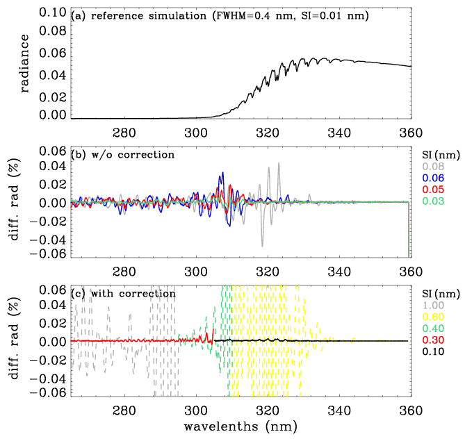
Figure 2 (a) Reference (truth) normalized radiance spectrum simulated at the spectral intervals (SIs) of 0.01 nm in 265–360 nm (solar zenith angle, SZA = 65^∘; viewing zenith angle, VZA = 30^∘; relative azimuth angle, AZA = 120^∘), which is used for evaluating the simulations in panels (b) and (c). (b) Impact of undersampling on the simulation. Panel (c) is similar to panel (b), but now the undersampling correction has been applied; the dashed and solid lines represent the sampling rates for v1 and v2, respectively. Note that individual radiances simulated at different SIs are interpolated to 0.01 nm and then convolved with the Gaussian function (FWHM: 0.4 nm) which represents the OMI instrument spectral response function.

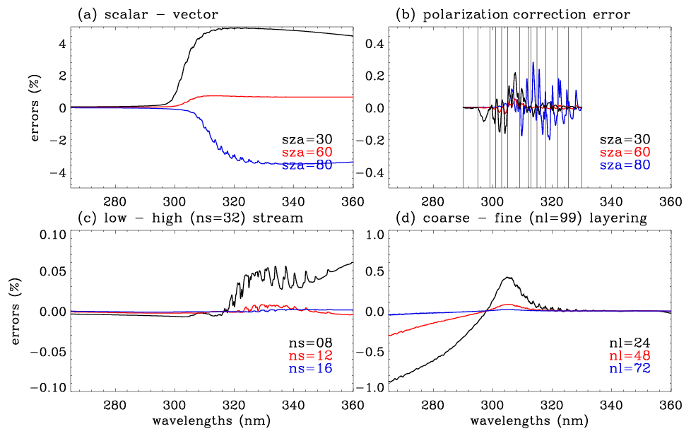
Figure 3 Errors of the radiance simulation due to the RT approximation used in v1, arising from (a) neglecting the polarization effect, (b) polarization correction errors (vertical lines indicate wavelengths at which the vector model is run for deriving the correction spectrum), (c) using a low number of streams (ns), and (d) using a coarse vertical layering (nl = number of layers). Note that this experiment is done at SZA = 65^∘, VZA = 30^∘, and AZA = 120^∘ if there is no specific notification.

3 The improved forward model scheme

The right panel of Fig. 1 illustrates the flowchart of the updated forward model scheme (v2) which employs the PCA-based RT model to perform online scalar simulations using four streams and a 24-layer atmosphere for RT performance enhancement (step 1) and two kinds of correction schemes for accounting for approximation errors (steps 2 and 3). Section 3.1.1 gives an overview on how the PCA tool is combined with the VLIDORT version 2.8 model; full theoretical details may be found in Spurr et al. (2016) and Kopparla et al. (2017). Here, our paper gives details on how the PCA-based RT configuration is optimized for the application to UV ozone profile retrievals for maximizing the speed-up in Sect. 3.1.2. Section 3.2 specifies step 2, wherein the LUT-based correction is applied to approximation errors due to the use of a scalar model, a smaller number of streams, and coarser-resolution vertical grid. In step 3 the undersampling correction is adopted from the v1 implementation, but the Rayleigh scattering term of the Eq. (1) is neglected for the speed up with trivial loss of accuracy.

3.1 PCA-based RT model

3.1.1 General PCA procedure

The PCA-based RT process begins with a grouping of spectral points into several bins; atmospheric profile optical properties within each bin are similar. PCA is a mathematical transformation that converts a correlated mean-subtracted dataset into a series of principal components (PCs). To enhance RT performance, PCA is used to compress a binned set of correlated optical profile data into a small set of atmospheric profiles which capture the vast majority of the data variance within the bin. The layer extinction optical thickness Δ_n,i and the single scattering albedos ω_n,i are generally subjected to PCA, where n and i are indices for atmospheric layers ($n=\mathrm{1},\mathrm{\cdots }{N}_{\mathrm{L}}$) and spectral points ($i=\mathrm{1},\mathrm{\cdots }{N}_{\mathrm{S}}$), respectively. For each bin, the optical profiles ln Δ_n,i and ln ω_n,i are composed of 2N_L×N_S matrix G in log space (${\mathbf{G}}_{n,i}=\ln {\mathrm{\Delta }}_{n,i}$, ${\mathbf{G}}_{n+N_{\mathrm{L}},i}=\ln {\mathit{\omega }}_{n,i}$). The mean-removed 2N_L×2N_L covariance matrix Y is then

$$\begin{array}{}\text{(2)}& \mathbf{Y}={\left[\mathbf{G}-\langle \mathbf{G}\rangle \right]}^T\left[\mathbf{G}-\langle \mathbf{G}\rangle \right],\end{array}$$

where 〈〉 denotes spectral averaging over all grid points in a bin. This covariance matrix Y is decomposed into eigenvalues ρ_k and unit eigenvectors X_k through solution of the eigenvalue problem YX_k=ρ_kX_k, where the index k runs from 1 to 2N_L. The scaled eigenvectors of the covariance matrix are defined as the empirical orthogonal function (EOF), ${\mathit{W}}_k=\sqrt{{\mathit{\rho }}_k}{\mathbf{X}}_k$, where the EOFs are ranked in descending order starting with those having the largest eigenvalues. The principal components (PCs) are the projections of the original data onto the eigenvectors, ${\mathit{P}}_k=\frac{\mathrm{1}}{\sqrt{{\mathit{\rho }}_k}}\mathbf{G}{\mathit{W}}_k$. The original dataset can then be expanded in terms of the mean value and a sum over all EOFs. As inputs to the RT simulation, the PCA-defined optical states are defined as F₀=exp [〈G〉] and ${\mathit{F}}_k^{\pm }={\mathit{F}}_{\mathrm{0}}\exp \left[\pm {\mathit{W}}_k\right]$, corresponding respectively to the mean value and to positive and negative perturbations from the mean value by an amount equal to the magnitude of kth EOF. Therefore, Δ_n,i and ω_n,i (i=1…N_S) are expressed as follows:

$$\begin{array}{}\text{(3)}& \begin{array}{rl}& {\mathit{F}}_{\mathrm{0}}=\left\{\begin{array}{l}{\mathrm{\Delta }}_{n,\mathrm{0}}\\ {\mathit{\omega }}_{n,\mathrm{0}}\end{array}\right\}\equiv \left\{\begin{array}{l}\exp \left[\frac{\mathrm{1}}{N_{\mathrm{s}}}{\sum }_{i=\mathrm{1}}^{N_{\mathrm{s}}}\ln {\mathrm{\Delta }}_{n,i}\right]\\ \exp \left[\frac{\mathrm{1}}{N_{\mathrm{s}}}{\sum }_{i=\mathrm{1}}^{N_{\mathrm{s}}}\ln {\mathit{\omega }}_{n,i}\right]\end{array}\right\};\\ & {\mathit{F}}_k^{\pm }=\left\{\begin{array}{l}{\mathrm{\Delta }}_{n,\pm k}\\ {\mathit{\omega }}_{n,\pm k}\end{array}\right\}\equiv \left\{\begin{array}{l}{\mathrm{\Delta }}_{n,\mathrm{0}}\exp \left[\pm W_{n,k}\right]\\ {\mathit{\omega }}_{n,\mathrm{0}}\exp \left[\pm W_{n+N_{\mathrm{L}},k}\right]\end{array}\right\}.\end{array}\end{array}$$

For those optical quantities not included in the PCA reduction but still required in the RT simulations, the spectral mean values for the bin are assumed, as long as they have smooth monotonic spectral dependency or else are constant over the bin range. In our application, the phase functions and phase matrices for Rayleigh scattering are derived from bin-average values of the depolarization factor. Surface Lambertian albedos are constant in the RT simulation, but the calculated radiance is later adjusted to account for first-order wavelength dependency using surface albedo weighting functions. For larger bins, it is possible to include the depolarization ratio or the Lambertian albedo as additional elements in the optical dataset subject to PCA; this was investigated in another context by Somkuti et al. (2017).

In the PCA-based RT package, three independent RT models are combined in order to generate the full-scattering intensity field (I_FULL) at each spectral point λ_i in a single bin as follows:

$$\begin{array}{}\text{(4)}& I_{\mathrm{FULL}}\left({\mathit{\lambda }}_i\right)\cong \left[I_{\mathrm{2}\mathrm{S}}\left({\mathit{\lambda }}_i\right)+I_{\mathrm{FO}}\left({\mathit{\lambda }}_i\right)\right]C\left({\mathit{\lambda }}_i\right).\end{array}$$

Two fast-RT models, the first order (FO) and 2STREAM (2S), are used to generate an accurate single scatter (SS) field (I_FO) and an approximate multiple scatter (MS) field (I_2S), respectively, for every spectral point. The scalar 2S model computes the radiation field with two discrete ordinates only. To derive the correction factors C(λ_i), we first compute (logarithmic) ratios of the full-scatter and 2S-based intensity fields calculated with PCA-derived optical states F₀ and ${\mathit{F}}_k^{\pm }$:

$$\begin{array}{}\text{(5)}& \begin{array}{rl}& J_{\mathrm{0}}=\ln \left[{\displaystyle \frac{I_{\mathrm{VLD}}\left({\mathit{F}}_{\mathrm{0}}\right)+I_{\mathrm{FO}}\left({\mathit{F}}_{\mathrm{0}}\right)}{I_{\mathrm{2}\mathrm{S}}\left({\mathit{F}}_{\mathrm{0}}\right)+I_{\mathrm{FO}}\left({\mathit{F}}_{\mathrm{0}}\right)}}\right]\\ & J_k^{\pm }=\left[{\displaystyle \frac{{\mathbf{I}}_{\mathrm{VLD}}\left({\mathit{F}}_k^{\pm }\right)+I_{\mathrm{FO}}\left({\mathit{F}}_k^{\pm }\right)}{I_{\mathrm{2}S}\left({\mathit{F}}_k^{\pm }\right)+I_{\mathrm{FO}}\left({\mathit{F}}_k^{\pm }\right)}}\right].\end{array}\end{array}$$

Intensity ratios at the original spectral points J(λ_i) are then obtained using a second-order central-difference expansion based on the PCA principal components P_ki:

$$\begin{array}{}\text{(6)}& \begin{array}{rl}J\left({\mathit{\lambda }}_i\right)& =J_{\mathrm{0}}+\sum _{k=\mathrm{1}}^{N_{\mathrm{EOF}}}{\displaystyle \frac{\left(J_k^{+}-J_k^{-}\right)}{\mathrm{2}}}{P}_{ki}\\ & +{\displaystyle \frac{\mathrm{1}}{\mathrm{2}}}\sum _{k=\mathrm{1}}^{N_{\mathrm{EOF}}}{\left(J_k^{+}-\mathrm{2}{J}_{\mathrm{0}}+J_k^{-}\right)}^{\mathrm{2}}{P}_{ki}^{\mathrm{2}}.\end{array}\end{array}$$

The correction factors C(λ_i)=exp [J(λ_i)] are then applied to the approximate simulation (I_2S(λ_i)+I_FO(λ_i)) according to Eq. (4) above. More details can be found in the literature (Natraj et al., 2005, 2010; Spurr et al., 2013, 2016; Kopparla et al., 2017).

So far, we have discussed generation of total intensity field, using values I_FO(λ_i) and I_2S(λ_i) from full-spectrum FO and 2S model calculation, as well as PCA-derived values I_VLD(F), I_2S(F), and I_FO(F) based on PCA-derived optical states $\mathit{F}=\mathit{\{}{\mathit{F}}_{\mathrm{0}},{\mathit{F}}_k^{\pm }\mathit{\}}$. The above procedure works with VLIDORT operating in scalar or vector mode; however, the 2S model is purely scalar and cannot be used if we want to establish PCA-RT approximations to the Q and U components of the Stokes vector with polarization present. Instead, we rely on just the VLIDORT and FO models and develop a PCA-RT scheme based on the differences between the $Q/U$ values calculated by VLIDORT and FO for monochromatic and PCA-derived calculations, with an additive correction factor instead of the logarithmic ratios in Eq. (6) above. This was first introduced in Natraj et al. (2010) and is discussed in detail in Spurr et al. (2016).

Of greater importance for us is the need to derive PCA-RT approximations to profile Jacobians (weighting functions of the total intensity with respect to ozone profile optical depths). A PCA-RT Jacobians scheme was developed by Spurr et al. (2013) for total column Jacobians in connection with the retrieval of total ozone; this scheme involved formal differentiation of the entire PCA-RT system as outlined above for the intensity field. This is satisfactory for bulk property Jacobians, but for profile Jacobians it is easier to write (Efremenko et al., 2014; Spurr et al., 2016)

$$\begin{array}{}\text{(7)}& K_{\mathrm{FULL}}^{\left(\mathit{\xi }\right)}\left({\mathit{\lambda }}_i\right)\cong \left[K^{\left(\mathit{\xi }\right)}\left({\mathit{\lambda }}_i\right)+K_{\mathrm{FO}}^{\left(\mathit{\xi }\right)}\left({\mathit{\lambda }}_i\right)\right]D^{\left(\mathit{\xi }\right)}\left({\mathit{\lambda }}_i\right).\end{array}$$

Here, $K^{\left(\mathit{\xi }\right)}\left({\mathit{\lambda }}_i\right)\equiv \frac{\partial I\left({\mathit{\lambda }}_i\right)}{\partial \mathit{\xi }}$, with similar definitions for the FO and VLIDORT partial derivatives with respect to a parameter ξ. The Jacobian correction factor D^(ξ)(λ_i)=exp [L^(ξ)(λ_i)] is determined using the same central-difference expansion as that in Equation (6), but with quantities

$$\begin{array}{}\text{(8)}& \begin{array}{rl}& L_{\mathrm{0}}^{\left(\mathit{\xi }\right)}=\ln \left[{\displaystyle \frac{K_{\mathrm{VLD}}^{\left(\mathit{\xi }\right)}\left({\mathit{F}}_{\mathrm{0}}\right)+K_{\mathrm{FO}}^{\left(\mathit{\xi }\right)}\left({\mathit{F}}_{\mathrm{0}}\right)}{K_{\mathrm{2}\mathrm{S}}^{\left(\mathit{\xi }\right)}\left({\mathit{F}}_{\mathrm{0}}\right)+K_{\mathrm{FO}}^{\left(\mathit{\xi }\right)}\left({\mathit{F}}_{\mathrm{0}}\right)}}\right];\\ & L_{\pm k}^{\left(\mathit{\xi }\right)}=\left[{\displaystyle \frac{K_{\mathrm{VLD}}^{\left(\mathit{\xi }\right)}\left({\mathit{F}}_k^{\pm }\right)+K_{\mathrm{FO}}^{\left(\mathit{\xi }\right)}\left({\mathit{F}}_k^{\pm }\right)}{K_{\mathrm{2}\mathrm{S}}^{\left(\mathit{\xi }\right)}\left({\mathit{F}}_k^{\pm }\right)+K_{\mathrm{FO}}^{\left(\mathit{\xi }\right)}\left({\mathit{F}}_k^{\pm }\right)}}\right]\end{array}\end{array}$$

in place of J₀ and $J_k^{\pm }$ in Eq. (5).

3.1.2 The binning scheme

The major performance saving is achieved by limiting full-MS VLIDORT calculations to those based on the reduced set of PCA-derived optical states F₀ and ${\mathit{F}}_k^{\pm }$. A general binning scheme has been developed over the shortwave region from 0.29 to 3.0 µm (Kopparla et al., 2016), whereby the entire region is divided into 33 specially chosen sub-windows encompassing the major trace gas absorption signatures; in each such sub-window there are 11 bins for grouping optical properties and up to four EOFs for each PCA bin treatment; with this scheme, radiance accuracies of 0.1 % can be achieved throughout the region. However, the binning scheme should be tuned to the specific application to get additional computational saving, and here we investigate the optimal set for spectral binning and the number of EOFs in the Hartley and Huggins ozone bands (265–360 nm).

Optical properties within each bin must be strongly correlated to reduce the number of EOFs required to attain a given accuracy. According to Kopparla et al. (2016), the UV region is divided at 340 nm, beyond which O₂–O₂ absorption must be considered. In our application, the spectral region 340–360 nm is further divided at 350 nm: in the first sub-window, ozone absorption is much stronger than O₂–O₂, while for the second (350–360 nm), O₂–O₂ absorption becomes dominant. The binning criteria are generally determined by similarities in total optical depth of gas absorption profiles τ_ij as defined below:

$$\begin{array}{}\text{(9)}& {\mathrm{\Gamma }}_{\mathrm{g}}=-\ln \sum _{i=\mathrm{1}}^{N_{\mathrm{L}}}\sum _{j=\mathrm{1}}^{N_{\mathrm{g}}}{\mathit{\tau }}_{ij},\end{array}$$

where N_L and N_g denote the number of atmospheric layers and atmospheric trace gases.

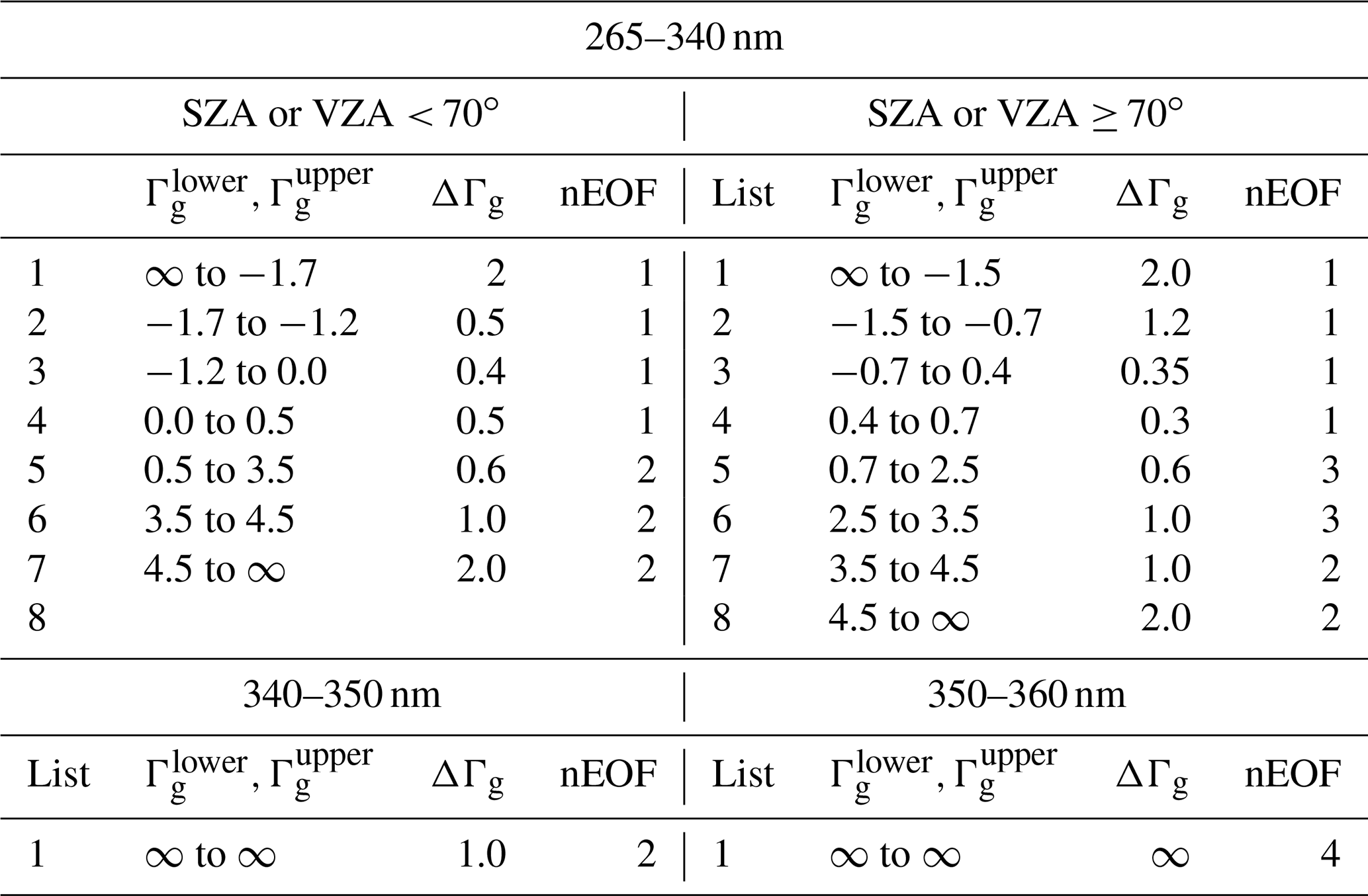
Table 1 The PCA-RT configuration optimized over the UV spectral range 265–360 nm. The optical depth of the total gas column (Γ_g defined in Eq. 9) is used to set the criteria for the spectral binning; for example, one or more bins are created at intervals (ΔΓ_g) in the range ${\mathrm{\Gamma }}_{\mathrm{g}}^{\mathrm{lower}}$ to ${\mathrm{\Gamma }}_{\mathrm{g}}^{\mathrm{upper}}$. For each bin, the optical states are expanded in terms of the first few number of EOFs (nEOF).

To evaluate the PCA approximation, the “exact-RT” model is performed, where accurate full-MS VLIDORT calculations are expensively performed at every wavelengths in addition to accurate SS calculations:

$$\begin{array}{}\text{(10)}& I_{\mathrm{exact}}\left({\mathit{\lambda }}_i\right)=I_{\mathrm{VLD}}\left({\mathit{\lambda }}_i\right)+I_{\mathrm{FO}}\left({\mathit{\lambda }}_i\right).\end{array}$$

We first evaluate the impact of applying different binning steps and numbers of EOFs in Fig. 4 where the residuals (I_PCA−I_EXACT) are plotted as a function of Γ_g for the spectral window 265–340 nm at small and large SZAs, respectively. In this evaluation, the bins are equally spaced in Γ_g for the five steps from 0.20 to 1.0. For Γ_g < 1, where the extinction is strong enough that radiances are very small, the residuals are effectively reduced by having more bins rather than increasing the number of EOFs. In this optical range, using the first EOF is enough to capture the vast majority of the spectral variance, with the optimization of the binning step. However, the bins should be narrowly spaced with Γ_g intervals of at least 0.3–0.4 for those spectral grids for which Γ_g is less than −2. These spectral grids are correlated with the Hartley band above ∼ 300 nm, where radiance values rapidly increase due to decreasing ozone absorption, but the spectral variations are almost unstructured. The rest of our spectral region corresponds to the Huggins band above 310 nm, where spectral variations are distinctly influenced by local maxima and minima of ozone absorption. In this spectral region, PCA approximation errors can be greatly reduced by increasing the number of EOFs. However, it is interesting to note that the PCA approximation is not further improved by using four EOFs instead of three (not shown here). Figure 4 also illustrates the dependence of the PCA performance on SZA in the spectral range below 340 nm: for example, when two EOFs are applied with the binning step 0.4, errors are within ±0.02 % at smaller SZA but increase up to ±0.03 % at larger SZA. Therefore, as listed in Table 1, two sets of binning criteria are determined to keep the accuracy within 0.05 % for any viewing geometry. Based on the experiments shown in Fig. 5, the binning criteria are determined for the other sub-windows listed in Table 1, namely 340–350 and 350–360 nm: the former is set with bins at intervals of 1 and using the first two EOFs, while the latter is divided into a single bin with the first four EOFs. Figure 6 illustrates the binning criteria thus determined, demonstrating that the PCA performance keeps accuracies within 0.03 % when various sets of SZAs, ozone profiles, and vertical layers are implemented.

Figure 4 Residuals (%) of the PCA-RT radiance in the wavelength range 265–340 nm compared to the exact-RT calculations, for different binning steps (different colors) and number of EOFs. Results are plotted as a function of Γ_g (logarithm of the total gas optical depth); VZA = 30^∘ and AZA = 120^∘ for SZAs of (a, b, c) 10^∘ and (d, e, f) 80^∘, respectively.

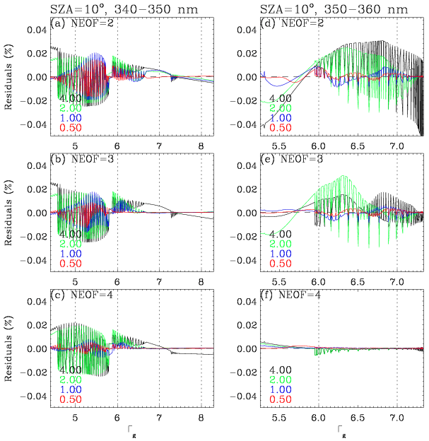
Figure 5 Same as Fig. 4 but for different windows: (a, b, c) 340–350 nm and (d, e, f) 350–360 nm, respectively.

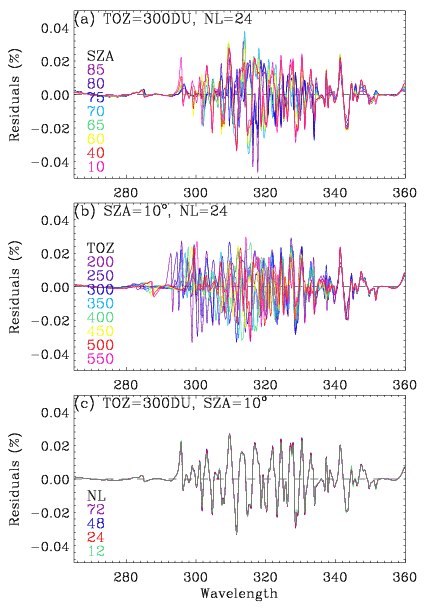
Figure 6 Residuals (%) of the PCA-RT radiances with the binning scheme given in Table 1 for various sets of (a) SZAs at VZA = 30^∘ and AZA = 120^∘, (b) ozone profiles with different total ozone columns (TOZs), and (c) number of atmospheric layers.

3.2 LUT-based correction

Two sets of LUTs are created: for high-accuracy (LUT_H: vector, 12 streams, 72 layers) and low-accuracy (LUT_L: scalar, 4 streams, 24 layers) configurations. The online PCA-VLIDORT model is configured to run in the LUT_L mode. The correction spectrum is straightforwardly calculated as the ratio of the LUT-based spectrum (LUT_H $/$ LUT_L), but the radiance correction term is additionally adjusted to account for the different gas optical depth profiles used in online and LUT simulations. The RT results are corrected for each wavelength as follows:

$$\begin{array}{}\text{(11a)}& {\displaystyle }\begin{array}{rl}{I}_{\mathrm{on}}& =I_{\mathrm{on},\mathrm{L}}\times \exp (\ln \left(I_{{\mathrm{LUT}}_{\mathrm{H}}}/I_{{\mathrm{LUT}}_{\mathrm{L}}}\right)\\ & +\sum _{n=\mathrm{1}}^{N_{\mathrm{L}}}[\left({{\displaystyle \frac{\partial \ln I}{\partial \mathit{\tau }}}}_{{\mathrm{LUT}}_{\mathrm{H}}}-{{\displaystyle \frac{\partial \ln I}{\partial \mathit{\tau }}}}_{{\mathrm{LUT}}_{\mathrm{L}}}\right)\\ & \times \left({\mathit{\tau }}_{\mathrm{on}}-{\mathit{\tau }}_{\mathrm{LUT}}\right)\left]\left(n\right)\right);\end{array}\text{(11b)}& {{\displaystyle \frac{\partial I}{\partial A_{\mathrm{s}}}}}_{\mathrm{on}}={{\displaystyle \frac{\partial I}{\partial A_{\mathrm{s}}}}}_{\mathrm{on},\mathrm{L}}\times {\displaystyle \frac{{\frac{\partial I}{\partial A_{\mathrm{s}}}}_{{\mathrm{LUT}}_{\mathrm{H}}}}{{\frac{\partial I}{\partial A_{\mathrm{s}}}}_{{\mathrm{LUT}}_{\mathrm{L}}}}};\text{(11c)}& {{\displaystyle \frac{\partial I}{\partial \mathit{\tau }}}}_{\mathrm{on}}={{\displaystyle \frac{\partial I}{\partial \mathit{\tau }}}}_{\mathrm{on},\mathrm{L}}\times {\displaystyle \frac{\partial I}{\partial {\mathit{\tau }}_{{\mathrm{LUT}}_{\mathrm{H}}}}}/{\displaystyle \frac{\partial I}{\partial {\mathit{\tau }}_{{\mathrm{LUT}}_{\mathrm{L}}}}},\end{array}$$

where the subscripts “on” and “LUT” stand for online and LUT-based calculations, respectively; A_s and τ_n represent the surface albedos and gas absorption optical depths (n is the layer index). To construct LUTs, RT calculations are performed using the VLIDORT version 2.8 model for sets of geometrical configurations (θ_o,θ; solar zenith angle, viewing zenith angle), surface pressures for 22 climatological ozone profiles, and 92 wavelengths (265–345 nm) as listed in Table 2. The azimuth dependence is treated exactly using the 0–2 Fourier intensity components in a Rayleigh scattering atmosphere in conjunction with the associated cosine-azimuth expansion of the full intensity; see the discussion below. The 22 ozone profiles are constructed from the GOME ozone profile product (Liu et al., 2005), where the ozone profile shapes vary according to three latitude regimes and with the total column ozone amounts at 50 DU intervals. The 92 wavelengths are regularly sampled at 5 nm intervals below 295 nm and at 1.0 nm intervals up to 310 nm in the Hartley band, while they are irregularly sampled at the local minima and maxima of the ozone absorption structures in the Huggins band. The results of these RT calculations are separated into two components: the path radiance I_atm and the surface reflectance term I_sfc according to Chandrasekhar (1960), so that the following relationship is employed to recover the full radiance:

$$\begin{array}{}\text{(12)}& \begin{array}{rl}I\left({\mathit{\theta }}_o,\mathit{\theta },\mathit{\phi }-{\mathit{\phi }}_o,A_{\mathrm{s}}\right)& =I_{\mathrm{atm}}\left({\mathit{\theta }}_o,\mathit{\theta },\mathit{\phi }-{\mathit{\phi }}_o\right)\\ & +I_{\mathrm{sfc}}\left({\mathit{\theta }}_o,\mathit{\theta },A_{\mathrm{s}}\right).\end{array}\end{array}$$

I_atm represents the purely atmospheric contribution to the radiance in the presence of a dark surface (zero albedo), and in a Rayleigh scattering atmosphere this is given as a Fourier expansion in the cosine of the relative azimuth angle.

$$\begin{array}{}\text{(13)}& \begin{array}{rl}{I}_{\mathrm{atm}}\left({\mathit{\theta }}_o,\mathit{\theta },\mathit{\phi }-{\mathit{\phi }}_{\mathrm{0}}\right)& =I_o\left({\mathit{\theta }}_o,\mathit{\theta }\right)+\cos \left(\mathit{\phi }-{\mathit{\phi }}_o\right)I_{\mathrm{1}}\left({\mathit{\theta }}_o,\mathit{\theta }\right)\\ & +\cos \mathrm{2}\left(\mathit{\phi }-{\mathit{\phi }}_o\right)I_{\mathrm{2}}\left({\mathit{\theta }}_o,\mathit{\theta }\right)\end{array}\end{array}$$

However, it is more convenient to write this in the form

$$\begin{array}{}\text{(14a)}& {\displaystyle }\begin{array}{rl}{I}_{\mathrm{atm}}& =I_{\mathrm{0}}\left({\mathit{\theta }}_o,\mathit{\theta }\right)\left(\mathrm{1}+k_{\mathrm{1}}\cos \left(\mathit{\phi }-{\mathit{\phi }}_o\right)Z_{\mathrm{1}}\left({\mathit{\theta }}_o,\mathit{\theta }\right)\right.\\ & \left.+k_{\mathrm{2}}\cos \mathrm{2}\left(\mathit{\phi }-{\mathit{\phi }}_o\right)Z_{\mathrm{2}}\left({\mathit{\theta }}_o,\mathit{\theta }\right)\right);\end{array}\text{(14b)}& {\displaystyle }\begin{array}{rl}& Z_{\mathrm{1}}\left({\mathit{\theta }}_o,\mathit{\theta }\right)={\displaystyle \frac{\mathrm{1}}{k_{\mathrm{1}}}}{\displaystyle \frac{I_{\mathrm{1}}\left({\mathit{\theta }}_o,\mathit{\theta }\right)}{I_{\mathrm{0}}\left({\mathit{\theta }}_o,\mathit{\theta }\right)}};\\ & Z_{\mathrm{2}}\left(\mathit{\theta },{\mathit{\theta }}_o\right)={\displaystyle \frac{\mathrm{1}}{k_{\mathrm{2}}}}{\displaystyle \frac{I_{\mathrm{2}}\left({\mathit{\theta }}_o,\mathit{\theta }\right)}{I_{\mathrm{0}}\left({\mathit{\theta }}_o,\mathit{\theta }\right)}};\end{array}\text{(14c)}& {\displaystyle }{k}_{\mathrm{1}}=-{\displaystyle \frac{\mathrm{3}}{\mathrm{8}}}\cos {\mathit{\theta }}_o\sin {\mathit{\theta }}_o\sin \mathit{\theta };k_{\mathrm{2}}={\displaystyle \frac{\mathrm{3}}{\mathrm{32}}}{\displaystyle \frac{{\left(\sin {\mathit{\theta }}_o\sin \mathit{\theta }\right)}^{\mathrm{2}}}{\cos \mathit{\theta }}}\end{array}$$

In the LUTs, the three coefficients (I₀, Z₁, and Z₂) are stored instead of I_atm. Note that the use of terms aq₁ and aq₂ is taken from Dave (1964); most of the angular variability in components I₁ and I₂ is captured analytically with these functions. In other words, Z₁ and Z₂ are angularly smooth and well-behaved (non-singular) functions, which helps improve angular interpolation accuracy with fewer points in the angular grids. The surface term is

$$\begin{array}{}\text{(15)}& I_{\mathrm{sfc}}\left({\mathit{\theta }}_o,\mathit{\theta },A_{\mathrm{s}}\right)={\displaystyle \frac{A_{\mathrm{s}}T\left({\mathit{\theta }}_o,\mathit{\theta }\right)}{\mathrm{1}-A_{\mathrm{s}}{s}^{\ast }}}.\end{array}$$

In the LUTs, we store the transmission term T(θ_o,θ), which is the product of the atmosphere downwelling flux transmittance for a solar source with the upwelling transmittance from a surface illuminated isotropically from below and the geometry-independent term s^∗ which is the spherical albedo from such a surface. This is the so-called “planetary problem” calculation (Chandrasekhar, 1960), and the code to obtain T and s^∗ is now implemented in VLIDORT version 2.8 (Spurr and Christi, 2019). One of the key features of the VLIDORT code is its ability to generate simultaneously (along with the Stokes vector radiation field) any set of Jacobians with respect to atmospheric and surface optical properties. VLIDORT also contains an analytical linearization of the planetary problem. Indeed, in our Rayleigh-based application, we require Jacobians with respect to the albedo A_s and the ozone profile elements τ. First, for the albedo weighting function we have straightforward differentiation from Eq. (15) as follows:

$$\begin{array}{}\text{(16)}& {\displaystyle \frac{\partial I}{\partial A_{\mathrm{s}}}}=T\left({\mathit{\theta }}_o,\mathit{\theta }\right){\left({\displaystyle \frac{q}{A_{\mathrm{s}}}}\right)}^{\mathrm{2}};q=A_{\mathrm{s}}/\left(\mathrm{1}-A_{\mathrm{s}}{s}^{\ast }\right).\end{array}$$

For the optical depth derivative, $\partial I/\partial \mathit{\tau }$ is calculated from

$$\begin{array}{}\text{(17)}& \begin{array}{rl}{\displaystyle \frac{\partial I}{\partial \mathit{\tau }}}& ={\displaystyle \frac{\partial I_{\mathrm{0}}}{\partial \mathit{\tau }}}+{\mathrm{aq}}_{\mathrm{1}}\cos \left(\mathit{\phi }-{\mathit{\phi }}_o\right){\displaystyle \frac{\partial Z_{\mathrm{1}}}{\partial \mathit{\tau }}}\\ & +{\mathrm{aq}}_{\mathrm{2}}\cos \mathrm{2}\left(\mathit{\phi }-{\mathit{\phi }}_o\right){\displaystyle \frac{\partial Z_{\mathrm{2}}}{\partial \mathit{\tau }}}+q{\displaystyle \frac{\partial T}{\partial \mathit{\tau }}}+T{\left(q\right)}^{\mathrm{2}}{\displaystyle \frac{\partial s^{\ast }}{\partial \mathit{\tau }}}.\end{array}\end{array}$$

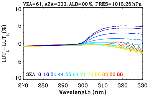
All partial derivatives in this expression are returned automatically by VLIDORT. For a given ozone profile, wavelength, and surface pressure, the number of the LUT values specified in Table 3 is 770 ($n\mathrm{Var}\times n{\mathit{\theta }}_o\times n\mathit{\theta }+S_{\mathrm{b}}+\frac{\mathrm{d}{S}_{\mathrm{b}}}{\mathrm{d}\mathit{\tau }}$, nVar=8: $I_{\mathrm{0}},Z_{\mathrm{1}},Z_{\mathrm{2}},T\frac{\mathrm{d}{I}_{\mathrm{0}}}{\mathrm{d}\mathit{\tau }}\frac{\mathrm{d}{Z}_{\mathrm{1}}}{\mathrm{d}\mathit{\tau }}\frac{\mathrm{d}{Z}_{\mathrm{2}}}{\mathrm{d}\mathit{\tau }},\frac{\mathrm{d}T}{\mathrm{d}\mathit{\tau }}$), which is much smaller than that of a LUT with dependence on eight relative azimuth angles and five surface albedo values (11 520 $=n\mathrm{Var}\times n{\mathit{\theta }}_o\times n\mathit{\theta }\times n\left(\mathit{\phi }-{\mathit{\phi }}_o\right)\times n{A}_{\mathrm{s}}$, nVar=3: $I,\partial I/\partial \mathit{\tau },\partial I/\partial A_{\mathrm{s}}$). LUT-based simulated radiances are evaluated against online simulations: the LUT interpolation errors are mostly less than 0.2 %–0.3 % (not shown here), except for extreme path length scenarios (e.g., ∼ 1 % at θ_o=87.0^∘) as shown in Fig. 7a, b; however, the interpolation errors are quite similar to each other for LUT_H and LUT_L. Therefore, those errors are canceled out when performing corrections using these two LUTs, and thereby the overall error after LUT correction is much smaller than ∼ 0.05 % (Fig. 7c). Note that the accuracy is completely maintained with respect to both φ−φ_o and A_s, while the size of a LUT is reduced by a factor of 15. However, LUT corrections still contain ozone profile shape errors due to the use of 22 representative total ozone-dependent ozone profiles in the LUT. Figure 8 shows an example of the correction spectrum as a function of SZA, showing that polarization errors are mostly dominant, except at the high SZAs above 310 nm, where errors due to use of a low number of streams become significant, and for wavelengths below 300 nm, where the use of the coarse vertical layering scheme becomes the main source of uncertainty.

Table 2 LUT parameter specification. Note that the relative azimuth dependence is taken into account explicitly through the Fourier coefficients of path radiance (Table 3), and the surface albedo dependence is taken into account by the planetary problem.

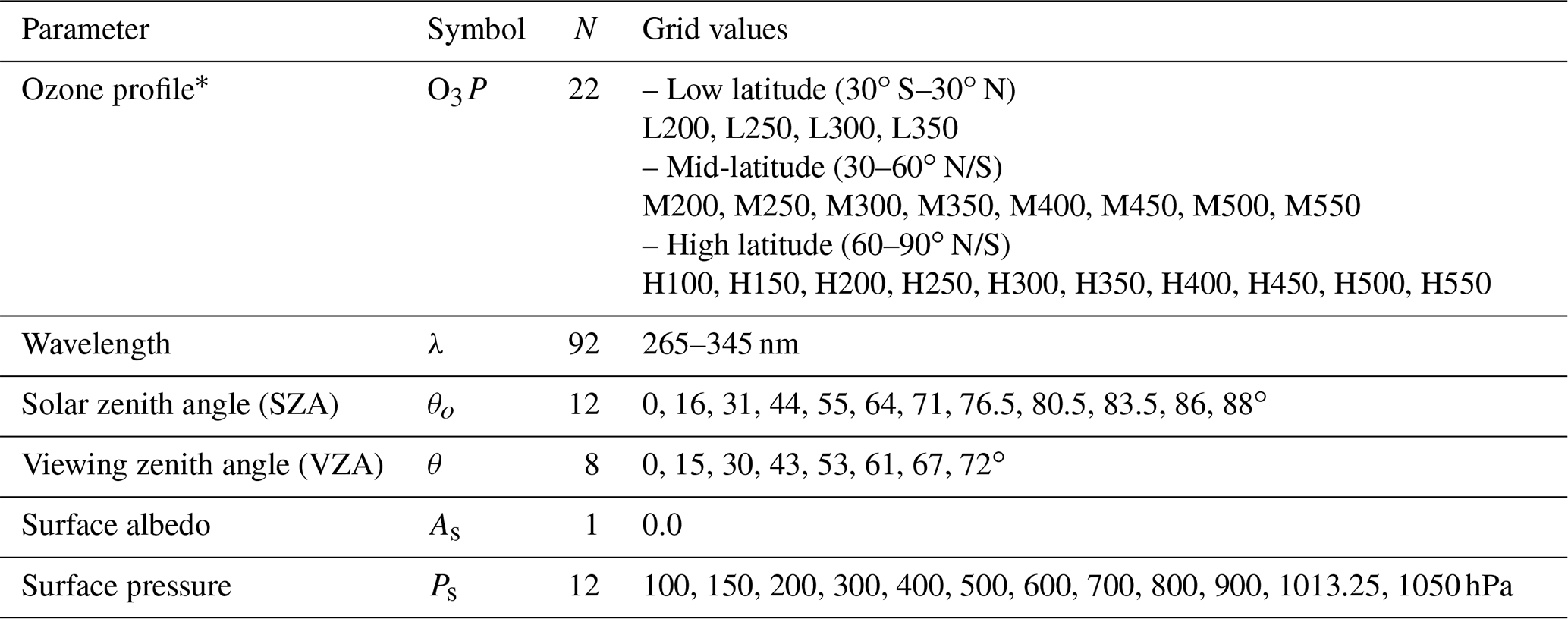
^∗ Total ozone-based ozone profiles for three latitude regimes. The grid values represent the amount of total ozone (DU).

Table 3 LUT variable specification.

^a Fourier coefficients of path radiance with respect to relative azimuth angle (AZA). ^b Total transmission of the atmosphere. ^c Spherical albedo of the atmosphere. ^d Total gas absorption optical depth profile. ^e n: number of atmospheric layers.

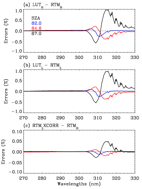
Figure 7 Comparisons of radiance simulations at VZA = 61^∘ and AZA = 0^∘ for extreme SZAs. LUT and RT model represent LUT- and online RT-based calculations, respectively, with the subscripts H and L indicating high- and low-accuracy configurations, whereas CORR represents the correction spectrum taken from LUT_H $/$ LUT_L.

Figure 8 Example of LUT-based correction spectrum.

4 Evaluation

The PCA-RT model developed as described in this paper is implemented as the forward model component of an iterative optimal-estimation-based inversion (Rodgers, 2000) for retrieving the ozone profile from OMI measurements. In previous studies, the PCA-RT performance was evaluated against a suite of exact monochromatic baselines of fully accurate VLIDORT simulations. However, such exact RT calculations cannot be applied in the operational data processing system, especially when thousands of spectral points are involved; in other words, the operational capability of the PCA-RT approach has been overestimated in previous studies. Therefore, we evaluate the RT model developed against the existing forward model where many RT approximations are applied to meet the computational budget in the operational system.

Table 4 List of configurations used in evaluating the different forward model calculations for OMI ozone profile retrievals. The reference, VLIDORT, and PCA-RT models are abbreviated as Ref, VLD, and PCA, respectively.

^a Undersampled (US) spectral intervals (nm) used to define wavelengths at which RT is actually executed. “0.3|0.1” represents the intervals divided at 305 nm, while for “1.0|0.4|0.6” those are divided at 295 and 310 nm. ^b High-resolution (HR) spectral intervals (nm) used to define wavelengths where undersampled simulations are interpolated before spectral convolution. ^c The number of discrete ordinates in the full polar space. ^d The number of atmospheric layers. ^e RT model is run in the vector (scalar) mode if polarization is true (false). ^f Online correction is performed for polarization errors, based on Liu et al. (2010). LUT-based correction is performed for RT approximation errors due to neglecting polarization as well as using four streams and 24 layers, developed in this study.

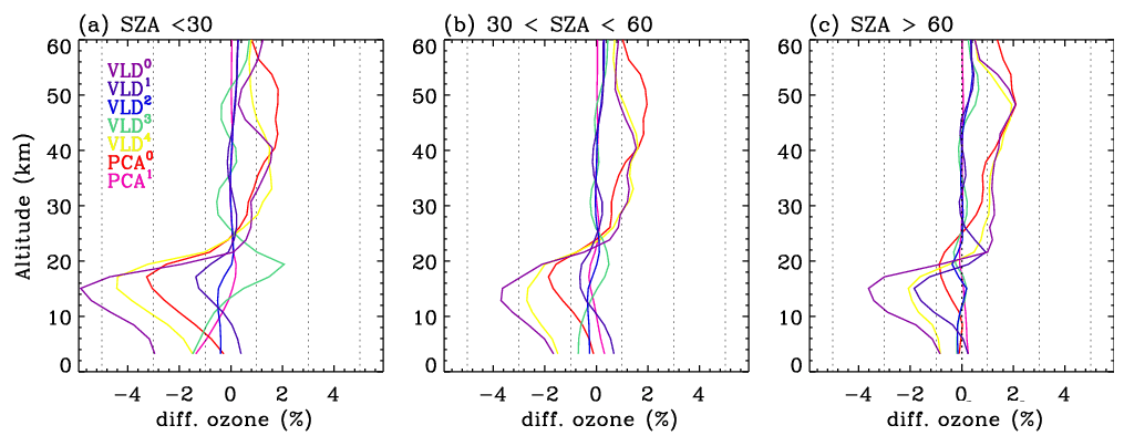
Figure 9 Mean biases of ozone profile retrievals with different configurations compared to those with the reference configuration. Each configuration is given in Table 4.

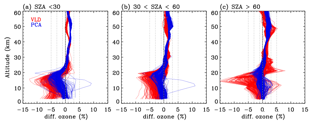
Figure 10 Same as Fig. 9 but for individual differences. VLD and PCA represent v1 and v2 forward model configurations, respectively.

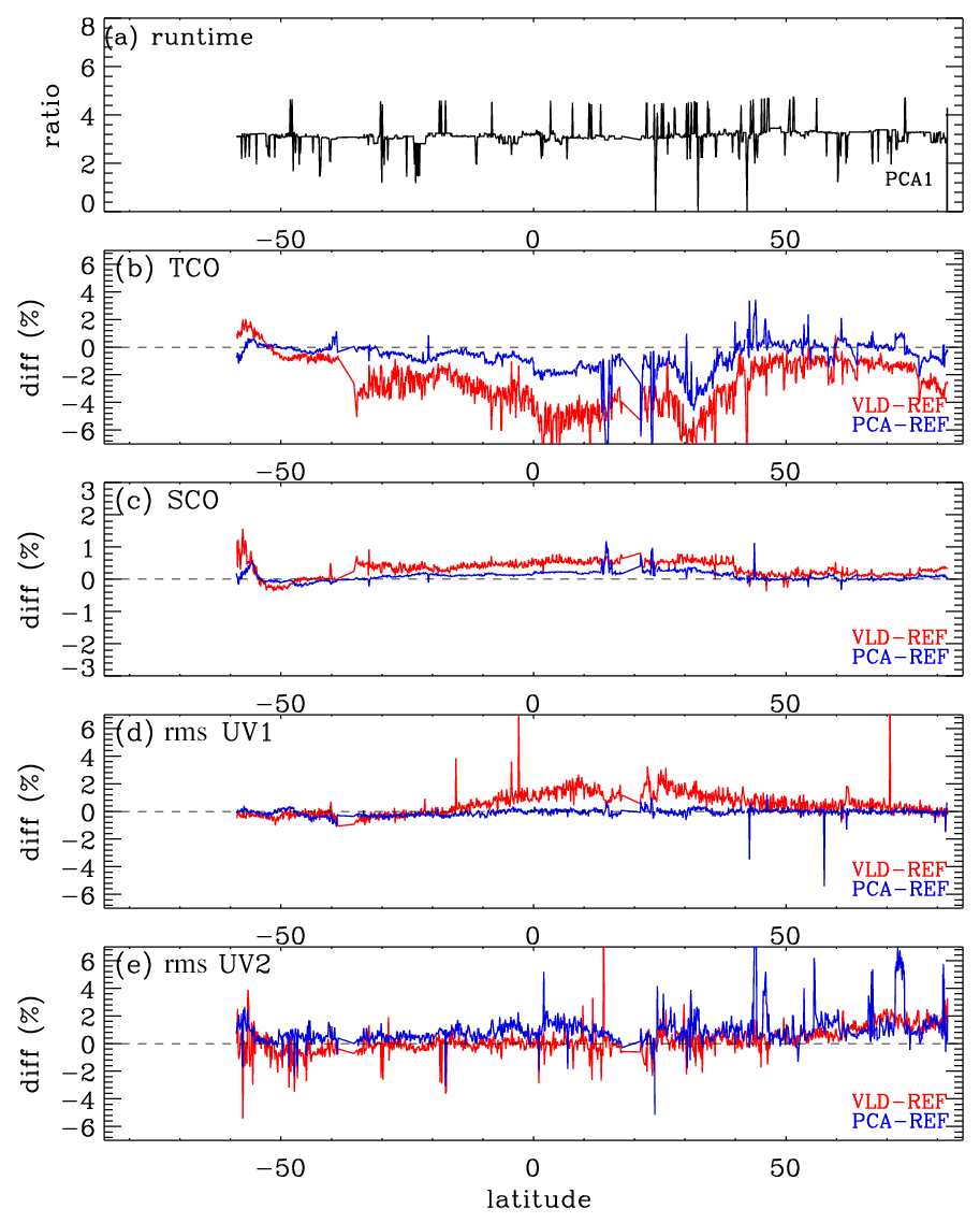
Figure 11 Same as Fig. 10 but for (a) runtime, (b) tropospheric column ozone (TCO), (c) stratospheric column ozone (SCO), and (d) UV1 (270–310 nm) and (e) UV2 (310–330 nm) fitting residuals, as a function of latitude at nadir cross-track. Note that the fitting residuals are estimated as root mean square (rms) errors for differences between measured and simulated spectra relative to the measurement error.

Table 4 contains sets of configurations for seven forward models. OMI spectra are simulated at the undersampled (US) intervals specified in the first column of this table and then interpolated at high-resolution (HR) intervals (second column) with the undersampling correction before convolution with OMI slit functions. In the v1 forward model, the US spectral intervals were set at 1.0 nm/0.4 nm intervals below/above 295 and 0.6 nm above 310 nm, while the HR spectral interval was set at 0.05 nm. In the updated RT model, the spectral points are selected at 0.3 nm (0.1 nm) intervals below (above) 305 nm, and the HR interval is set as 0.03 nm, which enables us to achieve very high accuracy, better than 0.01 %, as shown in Fig. 2c. In the reference configuration (abbreviated to “Ref”), VLIDORT is run in vector mode with 12 streams and 72 atmospheric layers so that the RT approximation errors are significantly reduced. The VLIDORT-based forward model is run with five sets of configurations (abbreviated to VLD in Table 4) to quantify the impact of RT approximations on ozone retrievals. Figure 9 compares the mean biases of the retrieved ozone profiles between VLD/PCA and Ref for three SZA regimes. VLD⁰ represents the v1 forward model configuration, demonstrating that the ozone retrieval errors due to the entire forward model errors range from ∼ 3.5 % for the large SZA regime to ∼ 5.5 % for the small SZA regime at the lower atmospheric layers but ∼ 2 % at the upper layers. The configuration VLD¹ assesses the impact of undersampling errors on the retrievals, causing negative biases of up to 2.0 % below ∼ 20 km. Compared to the use of 12 streams, using 8 streams causes negligible impacts on ozone retrievals (VLD²) as the corresponding RT model approximation errors are negligible, except for extreme viewing geometries where the ozone retrieval errors are overwhelmed by instrumental measurement errors (a few %) rather than the forward model errors of ∼ 0.05 % as shown in Fig. 3c. The VLD³-based RT calculation is applied to ozone retrievals for evaluating online polarization correction, showing that the corresponding errors in tropospheric ozone retrievals are estimated as ±2 % at small SZAs. The evaluation for VLD⁴ demonstrates that the use of coarse atmospheric layering causes the largest errors (∼ 4.5 % in the troposphere, ∼ 1.5 % in the stratosphere). PCA⁰ represents the v2 forward model configuration while PCA¹ is done with the highest accurate configuration except for PCA approximation. Retrieval errors due to PCA approximation are negligible except for the bottom few layers at smaller solar zenith angles (up to ∼ 1.5 %). Differences between PCA⁰ and PCA¹ represent the ozone retrieval errors due to LUT errors, mostly related to the profile shape errors between LUT and online calculations. In Fig. 10, the comparison between VLD (v1 PROFOZ) and PCA (v2 PROFOZ) is performed for individual ozone profile retrievals. The large systematic errors of ∼ 5 %–15 % due to v1 forward model errors are greatly eliminated below 30 km. In addition, the variabilities of individual differences are significantly eliminated over the entire layers at high solar zenith angles. However, there are still some remaining retrieval errors up to −5 % in the troposphere and 3 % in the stratosphere due to v2 forward model simulation errors. Figure 11 further evaluates the v2 implementation. First of all, the comparison of the runtime (Fig. 11a) demonstrates that v2 is faster by a factor of 3.3 on average. Some spectral fit residuals are eliminated in the UV 1 band over the middle area of the swath (low latitudes), where the SZAs are relatively small, by up to ∼ 2 %; the corresponding improvements are found in the stratospheric column ozone. The amount that the stratospheric column ozone deviated from the reference is reduced by ∼ 0.2 % with the v2 implementation. On the other hand, the tropospheric column ozone retrievals show improvements for most cases, whereas the fit residuals of the UV2 band are slightly worse in the low latitudes. Note that the smaller fitting residuals could not directly lead to better ozone retrievals likely due to the presence of systematic measurement errors.

5 Summary and conclusions

We have extended the PCA-based fast-RT method to improve computational challenges for OE-based SAO OMI ozone profile retrievals requiring iterative calculations of the radiance and its Jacobian derivatives. The PCA-RT model is designed to perform MS calculations for a few EOF-derived optical states which are developed from spectrally binned sets of inherent optical properties that possess some redundancy. In this study, the binning scheme is carefully turned for the UV ozone fitting window from 265 to 360 nm in such a way as to choose the number of EOFs to be as small as possible for each bin rather than always using the first four EOFs for all bins selected in previous studies. The spectral windows are divided into three sub-windows: (1) 265–340 nm, (2) 340–350 nm, and (3) 350–360 nm. Then, optical profiles are grouped into bins according to criteria based on the total gas optical depth, as specified in Table 1. We demonstrated that the PCA approximation errors for our application are within 0.03 % for any viewing geometry, optical depth profile, and vertical layering.

The existing (v1) forward model calculations are evaluated to determine the optimal configuration for the v2 forward model. RT approximation errors exist due to the use of 24 quite coarse vertical layers (2.5 km thick), which can cause radiance simulation errors of up to ∼ 1 % below 320 nm, and this leads to ozone retrieval errors of 2 %–4.5 % in the troposphere and 1.5 % in the stratosphere. Eight-stream calculations can result in radiance residuals of ∼ 0.05 % or less except at extreme viewing geometries, which causes trivial errors on ozone retrievals compared to other error factors. In spite of accounting for polarization errors using vector and scalar differences at 14 wavelengths, the retrieval accuracies are systematically worse by up to ∼ 2 % due to neglecting second-order polarization errors which are strongly correlated with ozone absorption features. We found that 72 atmospheric layers (∼ 0.7 km thick) and 12 streams should be used at least to improve the simulations comparable to those with 99 atmospheric layers and 32 streams. To reduce the impact of undersampling errors, we improve simulation intervals such as 0.3 nm below 305 nm and 0.1 nm above and thereby reduce the biases of the ozone retrievals by ∼ 1.5 % compared to the undersampled intervals used in the v1 simulation. Applying the PCA-RT approach allows us to reduce the number of MS calculations from the high-resolution optical dataset to 51 sets of EOF-derived optical states, but the performance savings are not enough to improve over previous RT approximations. To improve both efficiency and accuracy, we have developed a LUT-based correction for eliminating the RT approximation errors arising from the vector vs. scalar, 12 vs. 4 streams, and 72 vs. 24 layers. In conclusion, the updated PCA-based RT model combined with LUT corrections makes ozone profile retrievals faster than the v1 forward model by a factor of 3.3 on average. Fitting accuracies are significantly improved in the UV1 band by 2 % and comparable in the UV2 band, while the ozone profile retrievals are significantly improved, especially in the troposphere, by ∼ up to 10 %. However, there are still some remaining retrieval errors of up to −5 % in troposphere and 3 % in stratosphere due to the LUT correction errors and PCA approximation errors in the v2 implementation. The updated forward model is in preparation for reprocessing all OMI measurements (2004–current) for the next version of the PROFOZ product.