Quantitative imaging of volcanic SO₂ plumes using Fabry–Pérot interferometer correlation spectroscopy

We present first measurements with a novel imaging technique for atmospheric trace gases in the UV spectral range. Imaging Fabry–Pérot interferometer correlation spectroscopy (IFPICS) employs a Fabry–Pérot interferometer (FPI) as the wavelength-selective element. Matching the FPI's distinct, periodic transmission features to the characteristic differential absorption structures of the investigated trace gas allows us to measure differential atmospheric column density (CD) distributions of numerous trace gases with high spatial and temporal resolution. Here we demonstrate measurements of sulfur dioxide (SO₂), while earlier model calculations show that bromine monoxide (BrO) and nitrogen dioxide (NO₂) are also possible. The high specificity in the spectral detection of IFPICS minimises cross-interferences to other trace gases and aerosol extinction, allowing precise determination of gas fluxes. Furthermore, the instrument response can be modelled using absorption cross sections and a solar atlas spectrum from the literature, thereby avoiding additional calibration procedures, e.g. using gas cells. In a field campaign, we recorded the temporal CD evolution of SO₂ in the volcanic plume of Mt. Etna, with an exposure time of 1 s and 400×400 pixel spatial resolution. The temporal resolution of the time series was limited by the available non-ideal prototype hardware to about 5.5 s. Nevertheless, a detection limit of 2.1×10¹⁷ molec cm⁻² could be reached, which is comparable to traditional and much less selective volcanic SO₂ imaging techniques.

1 Introduction

Ground-based imaging of atmospheric trace gas distributions has a great potential to give new insights into mixing processes and chemical conversion of atmospheric trace gases by allowing their observation at high spatio-temporal resolution. Whereas present space-borne trace gas imaging provides daily global coverage with a spatial resolution of a few kilometres (e.g. Veefkind et al., 2012), ground-based observation can potentially reach a spatial resolution in the order of metres and a temporal resolution in the single digit Hz range. Such techniques in particular allow the investigation of trace gas distributions with strong gradients and short timescale chemical conversions.

There are several approaches for imaging trace gas distributions using scattered sunlight in the UV–Vis wavelength range (see, for example, Platt and Stutz, 2008; Platt et al., 2015): an image can be scanned pixel by pixel with a telescope, and recorded spectra are evaluated to determine the trace gas column density (whiskbroom approach). Alternatively, with a more complex optics and a two-dimensional detector, one detector dimension of the spectrograph can be used for spatially resolving an image column. Column by column (or pushbroom) scanning then resolves an image. The high spectral resolution of the spectrograph-based techniques allows the accurate and simultaneous identification of several trace gases; however, the light throughput and the scanning process severely limit the temporal resolution. A third approach applies tunable filters to resolve the trace gas spectral features, e.g. acousto-optical tunable filters (Dekemper et al., 2016), as wavelength-selective elements for an entire image frame. The application of tunable filters can have high spectral resolution and hence high trace gas selectivity; however, due to limited light throughput the temporal resolution lies in the order of minutes. A fourth imaging technique uses a small number (typically two) of wavelength channels selected by static filters, e.g. interference filters (Mori and Burton, 2006). This approach can be quite fast with a temporal resolution in the order of seconds; the trace gas selectivity, however, strongly depends on the correlation of trace gas absorption with the wavelength-selective elements and usually is rather marginal.

Fabry–Pérot interferometers (FPIs) exhibit a periodic spectral transmission pattern which can be matched to periodic spectral features (typically due to rotational or vibrational structures of electronic transitions) of the trace gas absorption, thereby yielding very high correlation for some trace gases. Imaging Fabry–Pérot interferometer correlation spectroscopy (IFPICS) thus essentially combines the advantage of fast image acquisition with selective spectral identification of the target trace gas. IFPICS was proposed by Kuhn et al. (2014) and discussed in Platt et al. (2015) for volcanic SO₂. Kuhn et al. (2019) demonstrated the feasibility with a 1 pixel prototype for volcanic SO₂ and evaluated its applicability to other trace gases.

Here we present first imaging measurements (at a resolution of 400×400 pixels, 1 s exposure time) performed with IFPICS and confirm its high selectivity and sensitivity. A prototype instrument for SO₂ was tested at Mt. Etna volcano, Italy, showing a noise-equivalent signal between 2.1×10¹⁷–5.5×10¹⁷ $\mathrm{molec}{\mathrm{cm}}^{-\mathrm{2}}{\mathrm{s}}^{-\mathrm{1}/\mathrm{2}}$. Furthermore, we show that the instrument response can be modelled and thereby intrinsically calibrated, using a solar atlas spectrum and literature trace gas absorption cross sections.

Existing interference-filter-based SO₂ cameras used, for example, for the quantification of volcanic trace gas emission fluxes into the atmosphere (Mori and Burton, 2006; Bluth et al., 2007; Kern et al., 2015a), exhibit strong cross-interferences to aerosol scattering extinction and other trace gases (Lübcke et al., 2013; Kuhn et al., 2014). Furthermore, these techniques require in-field calibration. Besides the thereby induced systematic errors that propagate into the emission flux quantification, the detection limit is mostly determined by these cross-interferences. Thus, the applicability of the technique is limited to strong emitters with respective plume and weather conditions. The much higher selectivity of IFPICS largely extends the range of applicable conditions (e.g. to ship emissions and weaker emitting volcanoes) and significantly reduces the systematic errors. Furthermore, the extension of the technique to other trace gases, e.g. bromine monoxide (BrO), formaldehyde (HCHO), or nitrogen dioxide (NO₂), can give new important insights into short-scale chemical conversion processes in the atmosphere.

2 Imaging Fabry–Pérot interferometer correlation spectroscopy (IFPICS)

Similarly to the SO₂ camera principle (e.g. Mori and Burton, 2006; Bluth et al., 2007), IFPICS uses an apparent absorbance (AA) $\stackrel{\mathrm{̃}}{\mathit{\tau }}={\mathit{\tau }}_A-{\mathit{\tau }}_B$, i.e. the difference between two measured optical densities τ_A and τ_B, to quantify the column density (CD) $S={\int }_{\mathrm{0}}^{L}c\left(l\right)\mathrm{d}l$, i.e. the integrated concentration c of the measured gas along a light path L for each pixel of the image. The AA is calculated from two (or more) spectral settings that yield a maximum correlation difference to the gas absorption spectrum. Ideally the periodicity of the FPI fringes is matched to periodic spectral absorption features as shown in Fig. 1 for SO₂. For IFPICS we use two spectral settings A and B. Setting A exhibits on-band absorption, where the FPI transmission maxima coincide with the SO₂ absorption maxima and hence correlate with the differential absorption structures of SO₂. Setting B uses an off-band position, where the FPI transmission maxima anti-correlate with the differential SO₂ absorption structures (see Fig. 1). The spectral separation between setting A and B is thereby reduced by a factor of ≈30 (in the case of SO₂) to only ≈0.5 nm in contrast to ≈10–15 nm for traditional SO₂ cameras (see Lübcke et al., 2013; Kern et al., 2015a), which minimises broadband interferences due to, for example, scattering and extinction by aerosols or other absorbing gases. This application of an FPI is similar to approaches reported by Wilson et al. (2007) and Vargas-Rodríguez and Rutt (2009), for the detection of carbon monoxide, carbon dioxide, and methane in the infrared spectral range.

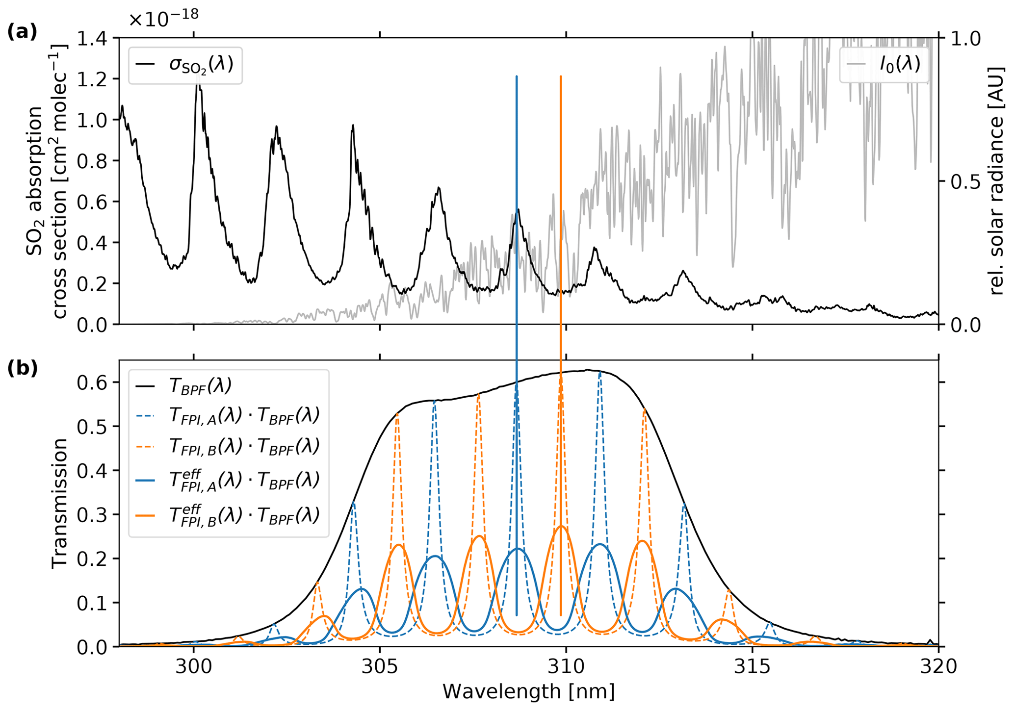
Figure 1 Spectral variation of (a) the SO₂ absorption cross section ${\mathit{\sigma }}_{{\mathrm{SO}}_{\mathrm{2}}}$ (black drawn, left axis, according to Bogumil et al., 2003) and the scattered skylight radiance I₀(λ) (grey drawn, right axis in relative units), given by Eq. (2). (b) The FPI transmissions in settings A and B yielding the maximum AA detectable (best correlation/anti-correlation to ${\mathit{\sigma }}_{{\mathrm{SO}}_{\mathrm{2}}}$) in the spectral range specified by the band pass filter used (BPF). The BPF transmission T_BPF(λ) (black) and the FPI transmission spectrum for a single-beam approach are shown according to Eq. (6) in on-band T_FPI,A(λ) (dashed blue, correlation with ${\mathit{\sigma }}_{{\mathrm{SO}}_{\mathrm{2}}}$) and off-band T_FPI,B(λ) setting (dashed orange, anti-correlation with ${\mathit{\sigma }}_{{\mathrm{SO}}_{\mathrm{2}}}$). The effective FPI transmission spectrum including an incident angle distribution is shown according to Eq. (7) in on-band $T_{\text{FPI},A}^{\text{eff}}\left(\mathit{\lambda }\right)$ (drawn blue) and off-band $T_{\text{FPI},B}^{\text{eff}}\left(\mathit{\lambda }\right)$ setting (drawn orange).

By measuring the optical density ${\mathit{\tau }}_A=\ln (I_A/I_{\mathrm{0},A})$ and ${\mathit{\tau }}_B=\ln (I_B/I_{\mathrm{0},B})$ in both spectral settings A and B respectively, the relation between the AA $\stackrel{\mathrm{̃}}{\mathit{\tau }}\left(S\right)$ with the CD S is given by

$$\begin{array}{ll}{\displaystyle }\stackrel{\mathrm{̃}}{\mathit{\tau }}\left(S\right)& {\displaystyle }={\mathit{\tau }}_A-{\mathit{\tau }}_B=-\log {\displaystyle \frac{I_A}{I_{\mathrm{0},A}}}+\log {\displaystyle \frac{I_B}{I_{\mathrm{0},B}}}=k\left(S\right)\\ \text{(1)}& {\displaystyle }& {\displaystyle }=\mathrm{\Delta }\stackrel{\mathrm{̃}}{\mathit{\sigma }}\left(S\right)\cdot S,\end{array}$$

where I_A and I_B denote the radiances with the presence of the target trace gas in the absorption light path and I_0,A and I_0,B the radiance without. The absorber-free reference radiances I_0,A and I_0,B can be determined from, for example, a reference region within the image. The differential weighted effective trace gas absorption cross section $\mathrm{\Delta }\stackrel{\mathrm{̃}}{\mathit{\sigma }}\left(S\right)$ becomes independent of S for small AAs ($\stackrel{\mathrm{̃}}{\mathit{\tau }}\ll \mathrm{1}$). At higher AAs, saturation effects occur due to the non-linearity of Lambert–Beer's law; however knowledge of the absorption cross sections, the background radiation spectrum, and the instrument transmission allows $\stackrel{\mathrm{̃}}{\mathit{\tau }}$ to be calculated for arbitrary CDs S using a numerical model.

2.1 Instrument model

The AA $\stackrel{\mathrm{̃}}{\mathit{\tau }}$ is modelled for given target trace gas CDs S by simulating the incoming radiances I_A and I_B and I_0,A and I_0,B. As incident radiation, a high-resolution, top of atmosphere (TOA) solar atlas spectrum I_0,TOA(λ) is used according to Chance and Kurucz (2010). The TOA spectrum is scaled by the wavelength λ⁻⁴ approximating a Rayleigh scattering atmosphere. Since our measurement wavelength range, of 304–313 nm for SO₂, overlaps with absorption of ozone (O₃), the TOA spectrum is corrected for the stratospheric O₃ absorption by multiplying all intensities by Lambert–Beer's term $e^{-{\mathit{\sigma }}_{{\mathrm{O}}_{\mathrm{3}}}\left(\mathit{\lambda }\right)\cdot S_{{\mathrm{O}}_{\mathrm{3}}}}$, where $S_{{\mathrm{O}}_{\mathrm{3}}}$ denotes the total atmospheric ozone slant column density, e.g. according to the TEMIS database (Veefkind et al., 2006), and ${\mathit{\sigma }}_{{\mathrm{O}}_{\mathrm{3}}}$ the O₃ absorption cross section according to Serdyuchenko et al. (2014). This yields the scattered skylight radiance I₀(λ) as follows:

$$\begin{array}{}\text{(2)}& {\displaystyle }{\displaystyle }{I}_{\mathrm{0}}\left(\mathit{\lambda }\right)=I_{\mathrm{0},\text{TOA}}\left(\mathit{\lambda }\right)\cdot e^{-{\mathit{\sigma }}_{{\mathrm{O}}_{\mathrm{3}}}\left(\mathit{\lambda }\right)\cdot S_{{\mathrm{O}}_{\mathrm{3}}}}\cdot f\left({\mathit{\lambda }}^{-\mathrm{4}}\right),\end{array}$$

indicated in Fig. 2. Based on I₀(λ), the radiances measured by the instrument for the two respective spectral settings are calculated with the absorption of trace gases and the spectral instrument transfer function T_instr(λ). The investigated target trace gas j (in this work SO₂) and potentially interfering trace gas species k (in this work O₃) are added according to Lambert–Beer's law. In the following we use the index i, denoting the FPI settings A and B, respectively. The quantity I_0,i thereby denotes the reference radiance excluding the target trace gas j from the light path (see Fig. 2).

$$\begin{array}{ll}{\displaystyle }& {\displaystyle }{I}_i=\int \mathrm{d}\mathit{\lambda }{I}_{\mathrm{0}}\left(\mathit{\lambda }\right)\cdot \exp \left(-{\mathit{\sigma }}_j\left(\mathit{\lambda }\right)S_j-\sum _k{\mathit{\sigma }}_k\left(\mathit{\lambda }\right)S_k\right)\\ \text{(3)}& {\displaystyle }& {\displaystyle }\cdot T_{\text{instr,}i}\left(\mathit{\lambda }\right)\text{(4)}& {\displaystyle }& {\displaystyle }{I}_{\mathrm{0},i}=\int \mathrm{d}\mathit{\lambda }{I}_{\mathrm{0}}\left(\mathit{\lambda }\right)\cdot \exp \left(-\sum _k{\mathit{\sigma }}_k\left(\mathit{\lambda }\right)S_k\right)\cdot T_{\text{instr,}i}\left(\mathit{\lambda }\right)\end{array}$$

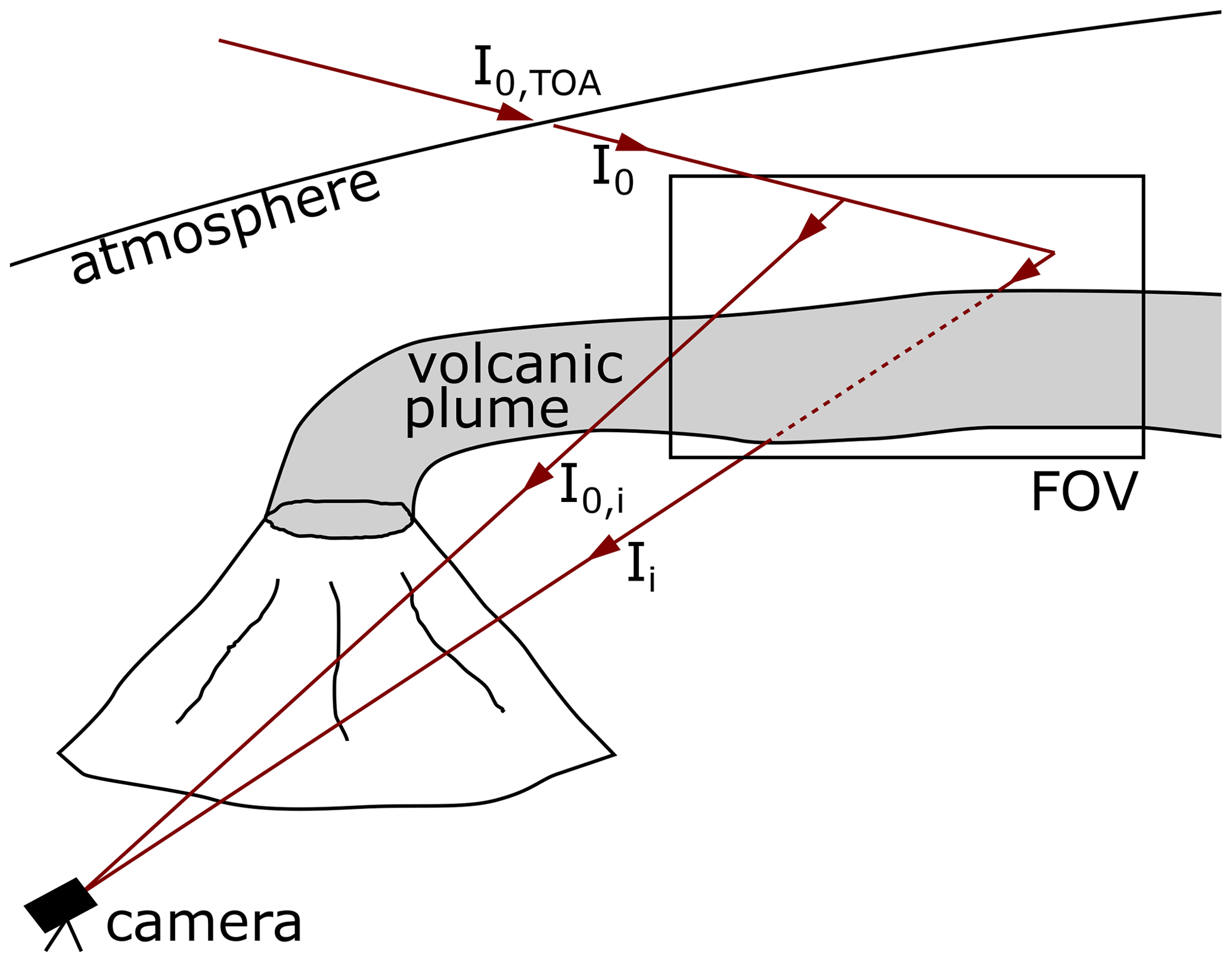
Figure 2 Schematic of the IFPICS measurement geometry, including the simulated radiances used in the instrument model. The incident top of atmosphere (TOA) radiation I_0,TOA is propagating through the atmosphere and is potentially scattered into the IFPICS camera field of view (FOV), yielding the scattered skylight radiance I₀. The camera records radiation in the respective FPI settings i=A and B that either traverses the volcanic plume I_i or originates from a plume-free area within the FOV I_0,i.

The spectral instrument transfer functions T_instr,i(λ) for the two spectral settings,

$$\begin{array}{}\text{(5)}& {\displaystyle }{\displaystyle }{T}_{\text{instr,}i}\left(\mathit{\lambda }\right)=T_{\text{FPI,}i}^{\text{eff}}\left(\mathit{\lambda }\right)\cdot T_{\text{BPF}}\left(\mathit{\lambda }\right)\cdot Q\left(\mathit{\lambda }\right)\cdot \mathit{\eta }\left(\mathit{\lambda }\right),\end{array}$$

consists of the measured band pass filter (BPF) transmission spectrum T_BPF(λ), the spectral (i.e. wavelength-dependent) quantum efficiency Q(λ) of the detector, and a spectral loss factor η(λ) of the employed optical components (e.g. by reflections). Considering only a single, parallel beam of light traversing the instrument, the FPI transmission spectrum T_FPI,i(λ) is defined by the Airy function (Perot and Fabry, 1899)

$$\begin{array}{ll}{\displaystyle }& {\displaystyle }{T}_{\text{FPI,}i}(\mathit{\lambda };{\mathit{\alpha }}_i,d,n,R)\\ \text{(6)}& {\displaystyle }& {\displaystyle }={\left[\mathrm{1}+{\displaystyle \frac{\mathrm{4}\cdot R}{(\mathrm{1}-R{)}^{\mathrm{2}}}}\cdot {\sin }^{\mathrm{2}}\left({\displaystyle \frac{\mathrm{2}\mathit{\pi }\cdot d\cdot n\cdot \cos {\mathit{\alpha }}_i}{\mathit{\lambda }}}\right)\right]}^{-\mathrm{1}}\end{array}$$

with the light beam incidence angle α_i for the two spectral settings onto the FPI, the FPI mirror separation d, the refractive index n of the medium inside the FPI, and the FPI reflectivity R (see Table 1, Figs. 1 and 3d). The FPI used in this work is static and air-spaced, meaning d, n, and R are fixed. Hence, the incidence angle α_i is the exclusive free parameter available to tune the FPIs transmission spectrum T_FPI,i between settings i=A and i=B respectively. The change in α_i is achieved by tilting the FPI optical axis with respect to the imaging optical axis (see Sect. 2.2).

However, in reality a spectral setting will always impinge with a range of incidence angles onto the FPI. In this work we assume cone-shaped light beams, with half cone opening angles ω_c, where the entire cone can be tilted by α_i relative to the normal of the FPI mirrors (see Fig. 3d). From this assumption, it follows that the incidence angles α_i are distributed over a cone with the incidence angle distribution $\mathit{\gamma }({\mathit{\alpha }}_i,{\mathit{\omega }}_{\mathrm{c}},\mathit{\vartheta },\mathit{\phi })$, where ϑ and φ are the polar and azimuth angles, respectively. Hence, the single-beam FPI transmission spectrum T_FPI,i(λ) of Eq. (6) is extended by a weighted average over $T_{\text{FPI,}i}(\mathit{\lambda };\mathit{\gamma }({\mathit{\alpha }}_i,{\mathit{\omega }}_{\mathrm{c}},\mathit{\vartheta },\mathit{\phi }),d,n,R)$, giving the effective FPI transmission spectrum $T_{\text{FPI,}i}^{\text{eff}}\left(\mathit{\lambda }\right)$:

$$\begin{array}{ll}{\displaystyle }& {\displaystyle }{T}_{\text{FPI,}i}^{\text{eff}}(\mathit{\lambda };\mathit{\gamma }({\mathit{\alpha }}_i,{\mathit{\omega }}_{\mathrm{c}}),d,n,R)={\displaystyle \frac{\mathrm{1}}{N\left(\mathit{\gamma }\right({\mathit{\alpha }}_i,{\mathit{\omega }}_{\mathrm{c}}\left)\right)}}\\ \text{(7)}& {\displaystyle }& {\displaystyle }\times \underset{\mathrm{0}}{\overset{{\mathit{\phi }}_{\text{max}}}{\int }}\underset{{\mathit{\vartheta }}_{\text{min}}}{\overset{{\mathit{\vartheta }}_{\text{max}}}{\int }}{T}_{\text{FPI,}i}(\mathit{\lambda };\mathit{\gamma }({\mathit{\alpha }}_i,{\mathit{\omega }}_{\mathrm{c}},\mathit{\vartheta },\mathit{\phi }),d,n,R)\sin \mathit{\vartheta }\mathrm{d}\mathit{\vartheta }\mathrm{d}\mathit{\phi }.\end{array}$$

Thereby, N(γ(α_i,ω_c)) denotes the weighting function with $N\left(\mathit{\gamma }\right({\mathit{\alpha }}_i,{\mathit{\omega }}_{\mathrm{c}}\left)\right)={\int }_{\mathrm{0}}^{{\mathit{\phi }}_{\text{max}}}{\int }_{{\mathit{\vartheta }}_{\text{min}}}^{{\mathit{\vartheta }}_{\text{max}}}\sin \mathit{\vartheta }\mathrm{d}\mathit{\vartheta }\mathrm{d}\mathit{\phi }$ given by the integral in Eq. (7), excluding the integrand T_FPI,i itself, ϑ the polar angle, and φ the azimuth angle of the spherical integration within boundaries defined by the tilted cone-shaped light beams. For example, for a non-tilted FPI (α_i=0) the integration boundaries are $\mathit{\vartheta }\in [\mathrm{0},{\mathit{\omega }}_{\mathrm{c}}]$ and $\mathit{\phi }\in [\mathrm{0},\mathrm{2}\mathit{\pi }]$; for a tilted FPI, however, the transformation of $\mathit{\gamma }({\mathit{\alpha }}_i,{\mathit{\omega }}_{\mathrm{c}},\mathit{\vartheta },\mathit{\phi })$ is more complex and requires several case analyses.

The incidence angle distribution γ(α_i,ω_c) will affect the shape of the FPI transmission spectrum by decreasing the effective finesse F of the FPI, leading to a blurring of the FPI fringes (see Fig. 1).

2.2 The IFPICS prototype

The IFPICS prototype is a newly developed instrument, designed to function under harsh environmental conditions in remote locations like, for example, in proximity to volcanoes. Hence, the prototype is designed to be small, with dimensions of $\mathrm{200}\mathrm{mm}\times \mathrm{350}\mathrm{mm}\times \mathrm{130}\mathrm{mm}$, lightweight at 4.8 kg (see Fig. 3a), and a power consumption <10 W; thus it can be battery-operated for several hours. A 2D UV-sensitive CMOS sensor with 2048×2048 pixel resolution (SCM2020-UV provided by EHD imaging) is used to acquire images. The sensor is operated in 4×4 binning mode, yielding a final image resolution of 512×512 pixels. However, we found that the software of the SCM2020-UV image sensor does not allow sufficiently precise triggering. Therefore ≈0.6 s is lost in each image acquisition, which severely limits the operation of the IFPICS camera. Replacement of the sensor by a scientific-grade UV detector array will solve this problem in future studies.

The internal camera optics is highly modular and easily adjustable. The IFPICS prototype employs an image side telecentric optical setup as proposed in Kuhn et al. (2014, 2019). A photograph and a schematic drawing are shown in Fig. 3. An aperture and a lens (lens 1) parallelise incoming light from the imaging field of view (FOV) before it traverses the FPI and the BPF. A second lens (lens 2) focusses the light onto the 2D UV-sensitive sensor. Thereby, in good approximation, all the pixels of the image experience the same spectral instrument transfer function T_instr,i(λ) for the two wavelength settings.

The FPI is the central optical element of the IFPICS prototype and is implemented as static air-spaced etalon with fixed d, n, and R (provided by SLS Optics Ltd.). The mirrors are separated using ultra-low expansion glass spacers to maintain a constant mirror separation d and parallelism over the large clear aperture of 20 mm, even in variable environmental conditions. In order to tune the spectral transmission $T_{\text{FPI}}^{\text{eff}}$ between setting A and B, a variation of the incidence angle α is applied. The FPI can be tilted within the parallelised light path using a stepper motor. The stepper motor has a resolution of 0.9^∘ per step, is equipped with a planetary gearbox (reduction rate 1∕9), and is operated in micro-stepping mode (1∕16), resulting in a resolution of 0.00625^∘ per motor step. The time required for tilting between our settings A and B is ≈0.15 s. We favour the approach of tilting the FPI over changing internal physical properties like, for example, the mirror separation d by piezoelectric actuators, as it keeps simplicity, robustness, and accuracy high for measurements under non-laboratory conditions. However it needs to be considered that the tilting of the FPI will generate a linear shift between the respective images acquired in setting A and B, requiring an alignment in the evaluation process.

The half cone opening angle ω_c is determined by the entrance aperture a and the focal length f of lens 1 and can be calculated by ${\mathit{\omega }}_{\mathrm{c}}=\arctan (a/\mathrm{2}f)$. The physical properties of the optical components and the instrument are listed in Table 1 and were mostly chosen according to the dimensioning assumed in the calculations of Kuhn et al. (2019).

The FPI design with fixed d, n, and R (see Fig. 3c) in particular is chosen to inherently generate a transmission spectrum matching the differential absorption structures of SO₂. This includes the basic idea that the untilted FPI (${\mathit{\alpha }}_i=\mathrm{0}{}^{\circ }$) already matches the on-band position A. In our case, however, the manufacturing accuracy of d lies within one free spectral range (≈2 nm for SO₂) so that ${\mathit{\alpha }}_B=\mathrm{0}{}^{\circ }$ corresponds to an off-band (B) position ($T_{\text{FPI},B}^{\text{eff}}$), and the on-band (A) position ($T_{\text{FPI},A}^{\text{eff}}$) is reached by a small tilt of ${\mathit{\alpha }}_A=\mathrm{4.5}{}^{\circ }$. The basic advantages of using small incident angles α_i are that they keep the spread of the incidence angle distribution γ(α_i,ω_c) (see Sect. 2.1) low and thereby retain the FPI's effective finesse F high (since the reflectivity R of the FPI mirror coating is somewhat dependent on the angle of incidence so is the finesse F). This leads to a much weaker blurring of the FPI fringes in the FPI transmission spectrum $T_{\text{FPI,}i}^{\text{eff}}$ resulting in a higher sensitivity of the instrument (see Fig. 1). With the prototype setup, however, we encountered disturbing reflections for low FPI incidence angles. For that reason we used the subsequent correlating order of the FPI transmission with ${\mathit{\alpha }}_A=\mathrm{8.17}{}^{\circ }$ for an on-band and ${\mathit{\alpha }}_B=\mathrm{6.45}{}^{\circ }$ for an off-band setting (see Table 1), thereby making a compromise between sensitivity and accurate evaluable images.

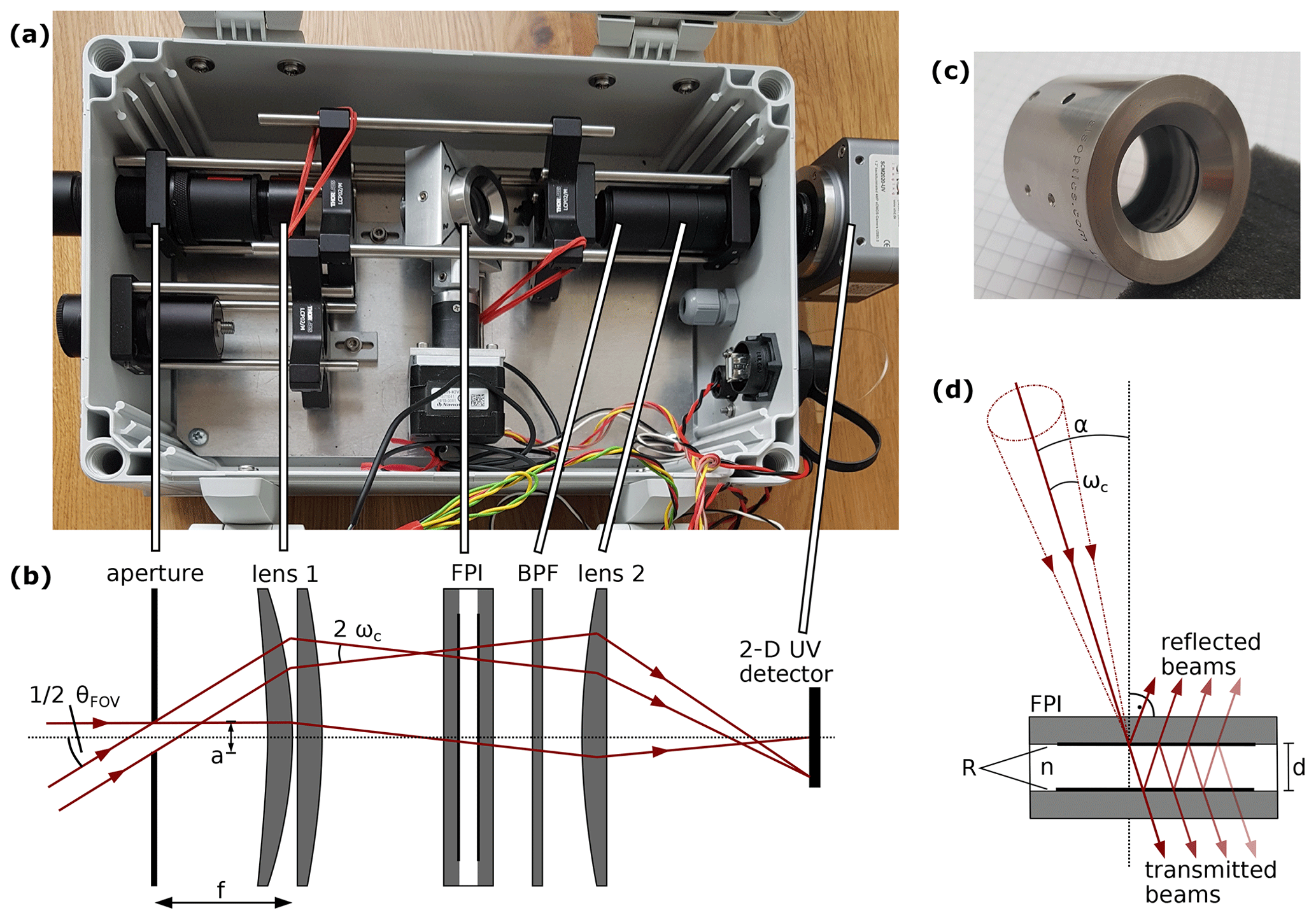
Figure 3 (a) Photograph of the IFPICS instrument. The physical dimensions are $\mathrm{200}\mathrm{mm}\times \mathrm{350}\mathrm{mm}\times \mathrm{130}\mathrm{mm}$ ($w\times l\times h$) and 4.8 kg. (b) Sketch of the image side telecentric optical setup of the IFPICS prototype. Incident radiation is parallelised by an entrance aperture and lens 1 before traversing the FPI and the band pass filter (BPF). The maximum half cone opening angle ω_c is dependent on the aperture diameter a and the focal length f of lens 1. The camera field of view is ${\mathit{\theta }}_{\text{FOV}}=\mathrm{18}{}^{\circ }$. A second lens maps the image onto a 2D UV-sensitive CMOS detector. (c) Photograph of the static air-spaced etalon (FPI) provided by SLS Optics Ltd. (d) Sketch of the FPI. An incoming single beam (drawn red) with incidence angle α is reflected multiple times between the FPI mirrors with reflectance R and separation d. Visualisation of an incoming cone-shaped beam (red dashed–dotted lines), with half cone opening angle ω_c and incidence angle α of the cone axis.

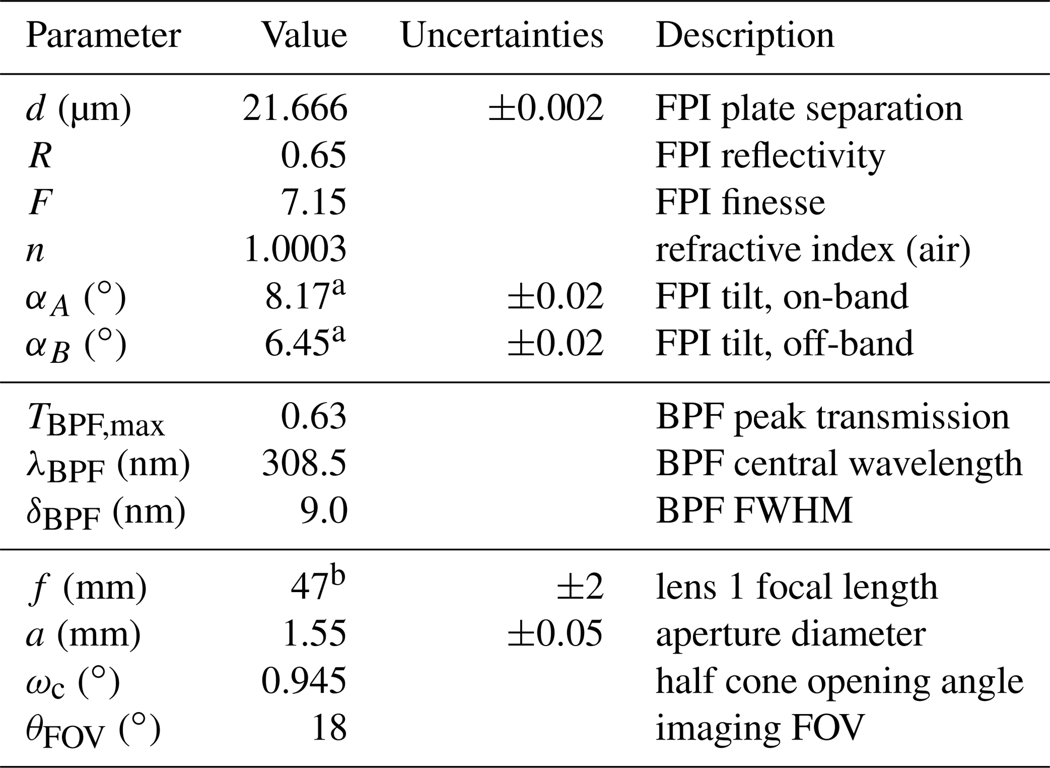
Table 1 Parameters of the optical components installed in the IFPICS prototype and used in the calibration model. The uncertainties of the model input parameters are shown.

^a Used in units of radian in the instrument model (Eqs. 6 and 7).
^b Two lenses: $f=\frac{f_{\mathrm{1}}\cdot f_{\mathrm{2}}}{f_{\mathrm{1}}+f_{\mathrm{2}}}$ with $f_{\mathrm{1}}=f_{\mathrm{2}}\approx \mathrm{94}\mathrm{mm}$ and λ=310 nm.

3 Proof of concept study

3.1 Measurements at Mt. Etna, Italy

First measurements with the prototype described above were performed at the Osservatorio Vulcanologico Pizzi Deneri (lat. 37.766, long. 15.017; 2800 $\mathrm{m}\mathrm{a}.\mathrm{s}.\mathrm{l}.$) at Mt. Etna, on 21 and 22 July 2019. The physical properties of the IFPICS prototype and the FPI tilt angles α_i for tuning $T_{\text{FPI,}i}^{\text{eff}}\left(\mathit{\lambda }\right)$ between on-band i=A and off-band setting i=B were selected according to Table 1. The tilt of the FPI generates a linear shift between the recorded on-band and off-band images on the detector and accounts for 6 pixels using tilt angles α_i. This shift needs to be corrected before cross-evaluating images recorded in setting A and B. The exposure time was set to 1 s for all measurements, and 4×4 binning (total spatial resolution of 512×512 pixels) was applied for all acquired images.

3.2 Validation of the instrument model

To quantify the accuracy of our model, two SO₂ gas cells were measured with the IFPICS prototype and by differential optical absorption spectroscopy (DOAS; see Platt and Stutz, 2008), on 21 July 2019, 11:10–11:20 CET. The sky was used as light source with a constant viewing angle (10^∘ elevation, 270^∘ N azimuth) in a plume-free part of the sky. To enhance the image quality, a flat-field correction is used, compensating pixel-to-pixel variations in sensitivity. The flat-field correction requires the acquisition of dark and flat-field images. The dark images are determined by the arithmetic mean over five images with no light entering the IFPICS instrument, and the flat-field images are obtained by the arithmetic mean over five images acquired in a plume-free sky region. The flat-field images thereby directly include the reference measurement I_0,i, making a later correction for the atmospheric background unnecessary. In the same viewing direction, I_i is measured for each gas cell and FPI setting i in order to calculate the AA according to Eq. (1). Figure 4 shows the gas cell measurements (red) including uncertainties (error bars, 1σ). The uncertainties directly arise from the errors of the DOAS measurement and due to variations in optomechanical settings of the IFPICS prototype.

The instrument model (Eqs. 2–7) was used to calculate the IFPICS AA ${\stackrel{\mathrm{̃}}{\mathit{\tau }}}_{{\mathrm{SO}}_{\mathrm{2}}}\left(S_{{\mathrm{SO}}_{\mathrm{2}}}\right)$ from a given SO₂ CD $S_{{\mathrm{SO}}_{\mathrm{2}}}$. The model parameters are mostly fixed by the IFPICS prototype optics, as given in Table 1. The remaining parameter, the atmospheric O₃ slant column density $S_{{\mathrm{O}}_{\mathrm{3}}}$ (see Eq. 2), is calculated in a geometric approximation $S_{{\mathrm{O}}_{\mathrm{3}}}={\text{VCD}}_{{\mathrm{O}}_{\mathrm{3}}}/\cos \left(\text{SZA}\right)$ using the solar zenith angle (SZA) and vertical O₃ column density (VCD${}_{{\mathrm{O}}_{\mathrm{3}}}$), which both are location-, date-, and time-dependent. They were $\text{SZA}=(\mathrm{53}\pm \mathrm{3}){}^{\circ }$ (according to the solar geometry calculator by NOAA, 2020) and VCD${}_{{\mathrm{O}}_{\mathrm{3}}}=(\mathrm{335}\pm \mathrm{5})\mathrm{DU}$ (according to the TEMIS database; Veefkind et al., 2006). The VCD${}_{{\mathrm{O}}_{\mathrm{3}}}$ can be treated to be approximately constant over the period of a day.

The output of the instrument model (drawn, black) for an SZA of 53^∘ is shown in Fig. 4. The model uncertainty (shaded grey) is determined by a root mean square over the errors in the output by individually varying the input parameters within their stated uncertainties. The thus calculated calibration function using the instrument model matches the SO₂ gas cells' validation measurement within the range of confidence. The model nicely describes the flattening of the AA–CD relation for high CDs (up to $\approx \mathrm{2.5}\times {\mathrm{10}}^{\mathrm{18}}\mathrm{molec}{\mathrm{cm}}^{-\mathrm{2}}$), which originates from the CD dependence of $\mathrm{\Delta }\stackrel{\mathrm{̃}}{\mathit{\sigma }}\left(S\right)$ (see Eq. 1).

To show the impacts of the SZA on the instrument model, the model output is also calculated for three other SZAs while keeping the other parameters constant. The model output is shown in Fig. 4 for an SZA of 80^∘ (dashed–dotted black) for early morning and late afternoon conditions, an SZA of 70^∘ (dashed black) for morning and afternoon conditions, and an SZA of 25^∘ (dotted black) for noon conditions. High SZAs lead to an increase of stratospheric O₃ absorption, which alters the spectral shape of the scattered skylight radiance I₀(λ) (see Eq. 2) which is used in the forward model. In other words, for high O₃ absorption, lower wavelength radiance, where the differential SO₂ absorption features are stronger, will contribute less to the integrated radiances I_i, I_0,i (Eqs. 3, 4). The thereby induced SZA dependence of the sensitivity can easily be accounted for in the model. Note that this influence of strong O₃ absorption only occurs at our chosen wavelength range for the SO₂ measurement. When applying IFPICS to other trace gases, e.g. BrO or NO₂, at higher wavelength, this effect will be negligible.

Figure 4 The validation measurement with two SO₂ gas cells (red, with 1σ error) with the IFPICS prototype and by DOAS on 21 July 2019, 11:10–11:20 CET, with a solar zenith angle (SZA) of 53^∘. The instrument forward model (Eqs. 2–7) is used to calculate the IFPICS AA ${\stackrel{\mathrm{̃}}{\mathit{\tau }}}_{{\mathrm{SO}}_{\mathrm{2}}}$ for a given CD $S_{{\mathrm{SO}}_{\mathrm{2}}}$ range. The model input parameters are shown in Table 1, and (335±5) DU is used as VCD${}_{{\mathrm{O}}_{\mathrm{3}}}$. The calculated model output (black) is shown for four different SZAs (25^∘, dotted; 53^∘, drawn; 70^∘, dashed and 80^∘, dashed–dotted). The model output and the validation measurement are in good agreement if a model SZA of 53^∘ is used, which is equivalent to the SZA during the measurement time. The model uncertainty is shown by the grey shading.

3.3 Results of the field measurements

Volcanic plume measurements were performed on 22 July 2019 at 08:50–09:10 CET. The instrument was pointing towards the plume of Mt. Etna's South-East Crater with a constant viewing direction (azimuth 204^∘ N, elevation 5^∘; see Fig. 5). The wind direction was ≈5^∘ N, with a velocity of $\approx \mathrm{6}\mathrm{m}{\mathrm{s}}^{-\mathrm{1}}$ (wind data from UWYO, 2020). Hence, the plume was partly covered by the crater flank. The frame rate during the measurement was 0.2 Hz for a pair (I_A and I_B) of images.

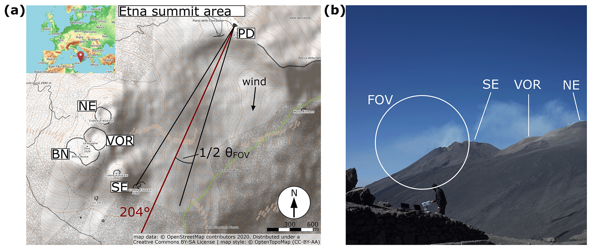
Figure 5 (a) Topographic map of the Mt. Etna summit area: North-East Crater (NE), Voragine (VOR), Bocca Nuova (BN), South-East Crater (SE), and measurement location at the Osservatorio Vulcanologico Pizzi Deneri (PD) are indicated. The viewing direction on 22 July 2019 is 204^∘ (red drawn) with a FOV of ${\mathit{\theta }}_{\text{FOV}}=\mathrm{18}{}^{\circ }$ (black drawn) and an elevation of 5^∘. The FOV is partly covering the plume emanating from SE crater. The average wind direction is $\approx \mathrm{5}{}^{\circ }$ with a speed of $\approx \mathrm{6}\mathrm{m}{\mathrm{s}}^{-\mathrm{1}}$ (wind data from UWYO, 2020). (b) Visual image of the volcanic plume on 22 July 2019 with camera field of view (FOV) indicated.

The flat-field correction was performed as described in Sect. 3.2, using the arithmetic mean over 10 dark images and five flat-field images, obtained in a plume-free sky region. An exemplary set of volcanic plume SO₂ images, obtained with the IFPICS instrument in on-band setting I_A and off-band setting I_B, are shown in Fig. 6. Further images of I_A and I_B are shown in Appendix A. The circular shape of the retrieved image arises from the FPI's circular clear aperture limiting the imaging FOV.

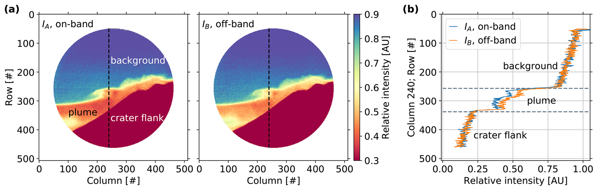
Figure 6 (a) Flat-field-corrected intensity images (400×400 pixels) acquired with the IFPICS prototype in on-band I_A and off-band setting I_B. The I_A image shows the expected higher SO₂ absorption in comparison with I_B (I_A<I_B in plume region). The plume is visible in both images due to the broadband SO₂ absorption and other extinction in the measurement spectral range. The circular image shape arise from the FPI's circular clear aperture. (b) Intensity column 240 (dashed black lines in a) for I_A (blue) and I_B (orange). The enhanced absorption (reduced intensity) is clearly visible in the plume section with I_A<I_B, whereas in the background sky and crater flank sections, the intensities are equal: I_A=I_B.

The IFPICS SO₂ AA ${\stackrel{\mathrm{̃}}{\mathit{\tau }}}_{{\mathrm{SO}}_{\mathrm{2}}}$ is calculated pixel-wise according to Eq. (1) from I_A and I_B. For the conversion into SO₂ CD $S_{{\mathrm{SO}}_{\mathrm{2}}}$, the forward instrument model (Eqs. 2–7) is inverted by least-squares fitting of a fourth-order polynomial to the calculated CD relation $S_{{\mathrm{SO}}_{\mathrm{2}}}\left({\stackrel{\mathrm{̃}}{\mathit{\tau }}}_{{\mathrm{SO}}_{\mathrm{2}}}\right)$. The model input parameters of the instrument are shown in Table 1. The SZA during the time of the measurement is $(\mathrm{78}\pm \mathrm{3}){}^{\circ }$ (NOAA, 2020), with a VCD${}_{{\mathrm{O}}_{\mathrm{3}}}$ of 335±5 DU (according to the TEMIS database; Veefkind et al., 2006). The retrieved calibration function $S_{{\mathrm{SO}}_{\mathrm{2}}}\left({\stackrel{\mathrm{̃}}{\mathit{\tau }}}_{{\mathrm{SO}}_{\mathrm{2}}}\right)$ is

$$\begin{array}{}\text{(8)}& {\displaystyle }{\displaystyle }{S}_{{\mathrm{SO}}_{\mathrm{2}}}\left({\stackrel{\mathrm{̃}}{\mathit{\tau }}}_{{\mathrm{SO}}_{\mathrm{2}}}\right)=\sum _{\mathrm{0}}^{\mathrm{4}}{x}_i\cdot {\stackrel{\mathrm{̃}}{\mathit{\tau }}}_{{\mathrm{SO}}_{\mathrm{2}}}^i,\end{array}$$

with $x_{\mathrm{0}}\stackrel{\mathrm{!}}{=}\mathrm{0},x_{\mathrm{1}}=\mathrm{1.8}\times {\mathrm{10}}^{\mathrm{19}}$, $x_{\mathrm{2}}=\mathrm{1.7}\times {\mathrm{10}}^{\mathrm{19}}$, $x_{\mathrm{3}}=\mathrm{1.7}\times {\mathrm{10}}^{\mathrm{19}}$, and $x_{\mathrm{4}}=\mathrm{6.6}\times {\mathrm{10}}^{\mathrm{19}}$ in units of molec cm⁻² respectively, with x₀ fixed to zero. This approximation yields an average relative deviation of 0.007 % for $S_{{\mathrm{SO}}_{\mathrm{2}}}$ from the modelled value, with a maximum relative deviation of 0.08 % for small SO₂ CDs.

An evaluated image of the volcanic plume SO₂ CD distribution corresponding to the intensities shown in Fig. 6 is shown in Fig. 7. Further evaluated CD distribution images of the same time series are presented in Appendix A. A time series of the plume evolution is visualised in a flip-book in the Supplement.

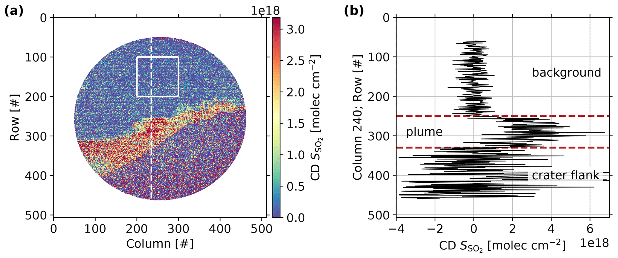
Figure 7 (a) Volcanic plume SO₂ CD distribution calculated from images acquired with the IFPICS prototype and using the instrument forward model conversion function $S_{{\mathrm{SO}}_{\mathrm{2}}}\left({\stackrel{\mathrm{̃}}{\mathit{\tau }}}_{{\mathrm{SO}}_{\mathrm{2}}}\right)$ (see Eq. 8). The plume-free area indicated by a white square (100×100 pixels) is used to correct for atmospheric background and to obtain an estimation for the detection limit. (b) Individual SO₂ CD column 240 (indicated by dashed white line in a) showing that the background, plume, and crater flank region are clearly distinguishable. High scattering in the crater flank region is induced by low radiance.

The volcanic plume of Mt. Etna's South-East Crater is clearly visibly and reaches SO₂ CDs higher than $\mathrm{3}\times {\mathrm{10}}^{\mathrm{18}}\mathrm{molec}{\mathrm{cm}}^{-\mathrm{2}}$. The atmospheric background is $S_{{\mathrm{SO}}_{\mathrm{2}},\text{bg}}=\mathrm{4.3}\times {\mathrm{10}}^{\mathrm{16}}\mathrm{molec}{\mathrm{cm}}^{-\mathrm{2}}$ and was determined by the arithmetic mean over a plume-free area within the evaluated image (white square, 100×100 pixels, in Fig. 7a). Since the $S_{{\mathrm{SO}}_{\mathrm{2}},\text{bg}}$ is determined from an evaluated CD distribution image, it accounts for the residual signal in $S_{{\mathrm{SO}}_{\mathrm{2}}}$ between the direction of the volcanic plume and the direction of the flat-field images used in the evaluation. The $S_{{\mathrm{SO}}_{\mathrm{2}},\text{bg}}$ was subtracted from the displayed image in the final step of the evaluation. The similar plume-free area (white square, 100×100 pixels, in Fig. 7a) is further used to give an estimation for the SO₂ detection limit of the IFPICS prototype by calculating the 1σ pixel–pixel standard deviation. The obtained detection limit for an exposure time of 1 s is 5.5×10¹⁷ molec cm⁻², given by the noise-equivalent signal. The measurements were performed in the morning with an SZA of 78^∘ and therefore reduced sensitivity and under relatively low light conditions. For decreasing SZA, the sensitivity will increase according to Fig. 4, and the increasing sky radiance will reduce the photon shot noise. In other words, the gas cell measurements (taken at SZA of 53^∘, with approximately twice the sky radiance compared to SZA of 78^∘) show a detection limit of $\mathrm{2.1}\times {\mathrm{10}}^{\mathrm{17}}\mathrm{molec}{\mathrm{cm}}^{-\mathrm{2}}$ for an exposure time of 1 s. For ideal measurement conditions (lowest SZA, highest sky radiance), the detection limit will be further improved.

After the proof of concept, showing the capability of IFPICS to determine SO₂ CD images, it is possible to determine fluxes from a CD image time series. In particular, if the series allows us to trace back individual features in consecutively recorded images, it can be used to directly determine the plume velocity using the approach of cross-correlation (e.g. McGonigle et al., 2005; Mori and Burton, 2006; Dekemper et al., 2016) or optical flow algorithms (e.g. Kern et al., 2015b) and to determine the plume propagation direction (e.g. Klein et al., 2017). However, the viewing geometry on the day of our measurement was unfavourable as it was not possible to reach another measurement location due to a lack of infrastructure. The plume propagation direction and central line of sight show an inclination of 19^∘ only, resulting in high pixel contortions, especially for pixels close to the edges of the FOV. Further, significant parts of the plume are covered by the crater flank due to its propagation direction. For the sake of completeness, we would like to give a rough estimate of the SO₂ flux obtained from our data.

The SO₂ flux ${\mathrm{\Phi }}_{{\mathrm{SO}}_{\mathrm{2}}}$ is determined by integrating the SO₂ CD along a transect through the volcanic plume and subsequent multiplication by the wind velocity perpendicular to the FOV direction; however due to the viewing geometry issues, we will use external wind data (direction: 5^∘; velocity $v_{\text{wind}}\approx \mathrm{6}\mathrm{m}{\mathrm{s}}^{-\mathrm{1}}$ data from UWYO, 2020) for the calculation. As the camera pixel size is finite, the integral is replaced by a discrete summation over the pixel n:

$$\begin{array}{}\text{(9)}& {\displaystyle }{\displaystyle }{\mathrm{\Phi }}_{{\mathrm{SO}}_{\mathrm{2}}}=v_{⟂}\sum _n{S}_{{\mathrm{SO}}_{\mathrm{2}},n}\cdot h_n,\end{array}$$

including the perpendicular wind velocity v_⟂, the SO₂ CD $S_{{\mathrm{SO}}_{\mathrm{2}},n}$, and the pixel extent h_n. The perpendicular wind velocity can directly be calculated from geometric considerations (see Fig. 5a), accounting to $v_{⟂}\approx \sin \left(\mathrm{19}{}^{\circ }\right)\cdot v_{\text{wind}}\approx \mathrm{2}\mathrm{m}{\mathrm{s}}^{-\mathrm{1}}$. To determine the pixel extent, the distance between the volcanic plume and the location of measurement is required. In the centre of the FOV, this distance is ≈3500 m, yielding h_n≈2.7 m. To keep the impact of pixel contortions low, the plume transect is located centrally in the FOV at column 250 and ranges from rows n=230 to 330. Using these quantities, we retrieve a mean SO₂ mass flux for the measurement of ${\mathrm{\Phi }}_{{\mathrm{SO}}_{\mathrm{2}}}=(\mathrm{84}\pm \mathrm{11})\mathrm{t}{\mathrm{d}}^{-\mathrm{1}}$ for the investigated plume of the South-East Crater, which is comparable to previous flux measurements of the South-East Crater (Aiuppa et al., 2008; D′Aleo et al., 2016). Nevertheless, the flux should be regarded as a lower limit, since the plume was covered by the crater flank to an unknown extent.

4 Conclusions

By imaging and quantifying the SO₂ distribution in the volcanic plume of Mt. Etna, we successfully demonstrate the feasibility of the IFPICS technique proposed by Kuhn et al. (2014). We were able to unequivocally resolve the dynamical evolution of SO₂ in a volcanic plume with a high spatial and temporal resolution (400×400 pixels, 1 s integration time, 4×4 binning). The retrieved detection limit for the SO₂ measurement is $\mathrm{5.5}\times {\mathrm{10}}^{\mathrm{17}}\mathrm{molec}{\mathrm{cm}}^{-\mathrm{2}}{\mathrm{s}}^{-\mathrm{1}/\mathrm{2}}$. The detection limit however varies with the SZA and can reach values below $\mathrm{2}\times {\mathrm{10}}^{\mathrm{17}}\mathrm{molec}{\mathrm{cm}}^{-\mathrm{2}}{\mathrm{s}}^{-\mathrm{1}/\mathrm{2}}$ under ideal conditions, comparable to traditional SO₂ imaging techniques (see Kern et al., 2015a). Also, the imaging technique lends itself to the determination of gas fluxes, and we obtained an SO₂ mass flux of ${\mathrm{\Phi }}_{{\mathrm{SO}}_{\mathrm{2}}}=(\mathrm{84}\pm \mathrm{11})\mathrm{t}{\mathrm{d}}^{-\mathrm{1}}$ for Mt. Etna's South-East Crater plume. However, due to unfavourable conditions in the viewing geometry, the retrieved flux should be treated as a lower limit. In general, it is possible to apply optical flow algorithms on image series acquired under more ideal viewing geometry conditions (e.g. Kern et al., 2015b). These allow the plume velocity and angle to be determined between the observation direction and plume propagation direction in order to retrieve accurate SO₂ fluxes (e.g. Klein et al., 2017).

The specific spectral detection scheme of IFPICS allows a numerical instrument model to be used to directly convert the measured AA $\stackrel{\mathrm{̃}}{\mathit{\tau }}$ into CD S distributions. This inherent calibration method makes in-field calibrations methods, e.g. by gas cells, unnecessary. The accuracy of the instrument model could be demonstrated using SO₂ cells with a known CD, determined by simultaneous DOAS measurements.

Our IFPICS instrument is still an early stage prototype. The optics employed is highly modular, allowing easy adjustments even outside a laboratory. The physical dimensions of <10 L and <5 kg and the low power consumption of <10 W, combined with the fact that no maintenance and in-field calibration are needed, make it already a close to ideal field instrument. Furthermore, the temporal resolution of the instrument can further be increased by replacing the sensor employed as it does not allow for time-optimised control of image acquisition.

Compared to traditional SO₂ cameras, the minimised cross-interferences to broadband plume extinction increase the selectivity and thus should allow to apply the IFPICS technique to much weaker SO₂ sources. Furthermore, the expected smaller interference to broadband effects in comparison to traditional SO₂ imaging techniques should allow the range of meteorological conditions acceptable for field measurement to be extended (see Kuhn et al., 2014).

The demonstrated IFPICS technique is not limited to the detection of SO₂. In general the technique is applicable to numerous further trace gases which show a distinct pattern (ideally periodic) in their absorption spectrum (see Kuhn et al., 2019). In the case of volcanic emissions, detectable trace species are, for example, bromine monoxide (BrO) or chlorine dioxide (OClO). Beyond volcanic applications IFPICS could be used to investigate, for example, air pollution by measuring nitrogen dioxide (NO₂) or formaldehyde (HCHO).

Appendix A:  

Further evaluated images of the time series acquired on 22 July 2019 at 08:50–09:10 CET at Mt. Etna, Italy, are shown in Fig. A1. The evaluation procedure is analogous to the routine explained in Sect. 3.3. The time difference between a set (1–4) of images accounts for ≈120 s and allows us to trace back plume dynamics.

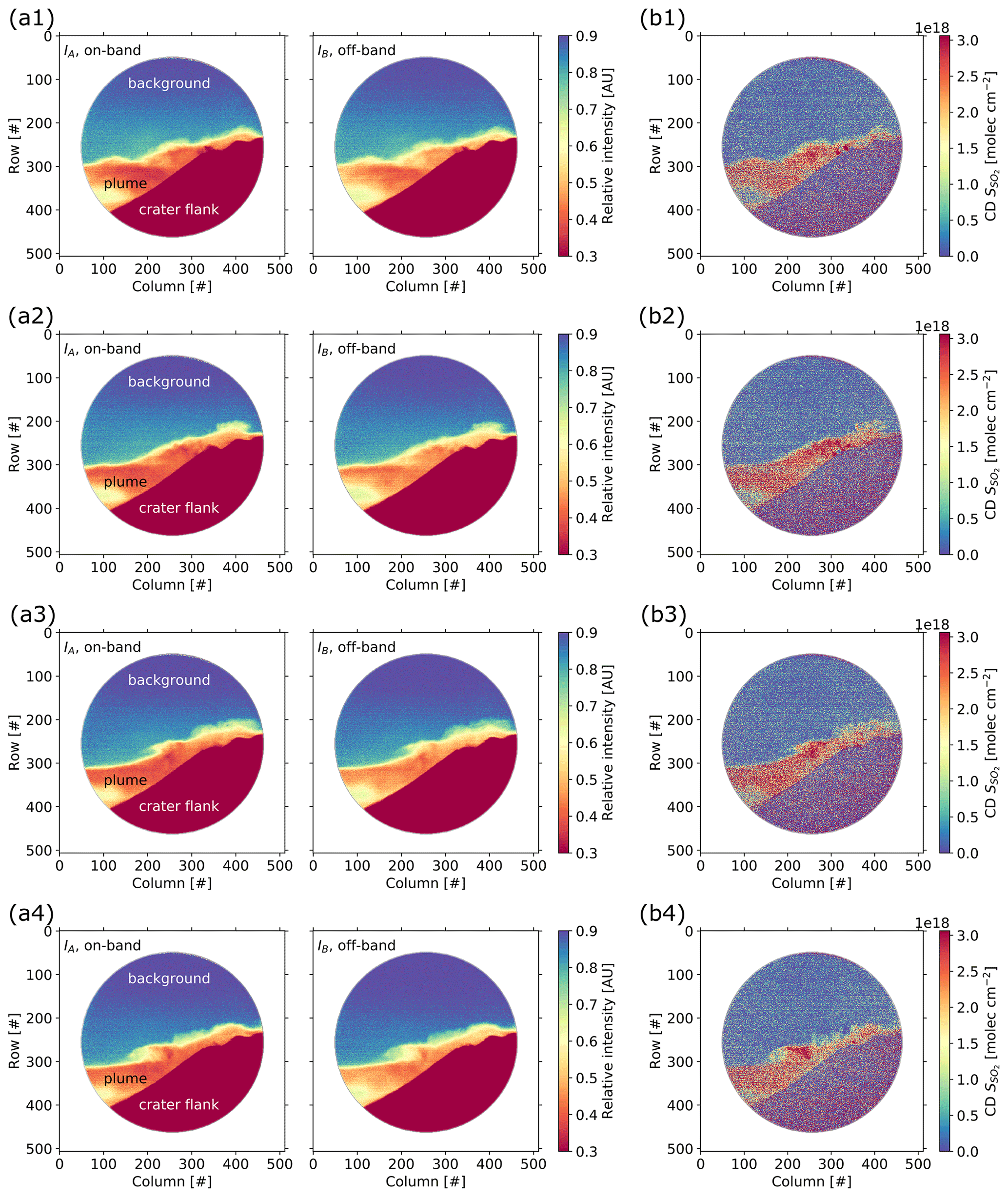
Figure A1 Exemplary set of evaluated images (400×400 pixels) acquired with the IFPICS prototype on 22 July 2019 at 08:50–09:10 CET at Mt. Etna, Italy. The time difference between each set of images (1–4) accounts for ≈120 s, allowing us to trace back plume dynamics. (a) Flat-field-corrected intensity images I_A and I_B. (b) Volcanic plume SO₂ CD $S_{{\mathrm{SO}}_{\mathrm{2}}}$ distribution calculated with the conversion function shown in Eq. (8).