Long-term NO_x measurements in the remote marine tropical troposphere

Atmospheric nitrogen oxides (NO + NO₂ = NO_x) have been measured at the Cape Verde Atmospheric Observatory (CVAO) in the tropical Atlantic (16^∘51^′ N, 24^∘52^′ W) since October 2006. These measurements represent a unique time series of NO_x in the background remote troposphere. Nitrogen dioxide (NO₂) is measured via photolytic conversion to nitric oxide (NO) by ultraviolet light-emitting diode arrays followed by chemiluminescence detection. Since the measurements began, a blue light converter (BLC) has been used for NO₂ photolysis, with a maximum spectral output of 395 nm from 2006 to 2015 and of 385 nm from 2015 onwards. The original BLC used was constructed with a Teflon-like material and appeared to cause an overestimation of NO₂ when illuminated. To avoid such interferences, a new additional photolytic converter (PLC) with a quartz photolysis cell (maximum spectral output also 385 nm) was implemented in March 2017. Once corrections are made for the NO₂ artefact from the original BLC, the two NO₂ converters are shown to give comparable NO₂ mixing ratios (BLC = 0.99 × PLC + 0.7 ppt, linear least-squares regression), giving confidence in the quantitative measurement of NO_x at very low levels. Data analysis methods for the NO_x measurements made at CVAO have been developed and applied to the entire time series to produce an internally consistent and high-quality long-term data set. NO has a clear diurnal pattern with a maximum mixing ratio of 2–10 ppt during the day depending on the season and ∼ 0 ppt during the night. NO₂ shows a fairly flat diurnal signal, although a small increase in daytime NO_x is evident in some months. Monthly average mixing ratios of NO₂ vary between 5 and 30 ppt depending on the season. Clear seasonal trends in NO and NO₂ levels can be observed with a maximum in autumn and winter and a minimum in spring and summer.

1 Introduction

Atmospheric nitrogen oxides play a key role in tropospheric chemistry. NO_x helps to control the abundance of the two most important oxidants in the atmosphere, ozone (O₃) and the hydroxyl radical (OH). The presence of NO is usually the key limiting factor in the production of tropospheric O₃, which occurs via oxidation of NO to NO₂ by peroxy radicals (RO₂, HO₂) as described in Reactions (R1)–(R2), followed by photolysis of NO₂ and rapid conversion of the resulting O(³P) to O₃.

$$\begin{array}{}\text{(R1)}& {\displaystyle }{\mathrm{RO}}_{\mathrm{2}}+\mathrm{NO}\to \mathrm{RO}+{\mathrm{NO}}_{\mathrm{2}}\text{(R2)}& {\displaystyle }{\mathrm{HO}}_{\mathrm{2}}+\mathrm{NO}\to \mathrm{OH}+{\mathrm{NO}}_{\mathrm{2}}\text{(R3)}& {\displaystyle }{\mathrm{NO}}_{\mathrm{2}}+h\mathit{\nu }\to \mathrm{NO}+\mathrm{O}{(}^{\mathrm{3}}\mathrm{P})(h\mathit{\nu }\le \mathrm{410}\mathrm{nm})\text{(R4)}& {\displaystyle }\mathrm{O}{(}^{\mathrm{3}}\mathrm{P})+{\mathrm{O}}_{\mathrm{2}}+\mathrm{M}\to {\mathrm{O}}_{\mathrm{3}}+\mathrm{M}\end{array}$$

Reaction (R2) also offers a route to the OH radical above its primary production via O₃ photolysis (Reactions R5 and R6). If the NO_x mixing ratio is sufficiently low, then peroxy radicals react with themselves instead of NO, and O₃ depleting reactions (Reactions R5–R8) dominate over O₃ production (Atkinson, 2000).

$$\begin{array}{}\text{(R5)}& {\displaystyle }{\mathrm{O}}_{\mathrm{3}}+h\mathit{\nu }\to \mathrm{O}{(}^{\mathrm{1}}\mathrm{D})+{\mathrm{O}}_{\mathrm{2}}(h\mathit{\nu }\le \mathrm{335}\mathrm{nm})\text{(R6)}& {\displaystyle }\mathrm{O}{(}^{\mathrm{1}}\mathrm{D})+{\mathrm{H}}_{\mathrm{2}}\mathrm{O}\to \mathrm{2}\mathrm{OH}\text{(R7)}& {\displaystyle }\mathrm{OH}+{\mathrm{O}}_{\mathrm{3}}\to {\mathrm{HO}}_{\mathrm{2}}+{\mathrm{O}}_{\mathrm{2}}\text{(R8)}& {\displaystyle }{\mathrm{HO}}_{\mathrm{2}}+{\mathrm{O}}_{\mathrm{3}}\to \mathrm{OH}+\mathrm{2}{\mathrm{O}}_{\mathrm{2}}\end{array}$$

It is assumed that, under tropospheric conditions at the low mole fractions discussed, NO and NO₂ behave as ideal gases and therefore mole fraction (picomole or mole, the appropriate SI unit) is equivalent to volumetric mixing ratio, represented by part per trillion (ppt). NO_x mixing ratios below 10–30 ppt are generally sufficiently low for net tropospheric O₃ depletion (Atkinson, 2000; Jaeglé et al., 1998; Logan, 1985). These conditions have previously been reported to apply most of the year in the remote Atlantic Ocean (Lee et al., 2009). The mixing ratio of NO_x in the atmosphere varies from a few ppt in remote areas (Lee et al., 2009; Monks et al., 1998; Reed et al., 2017) to > 100 ppb in polluted areas (Berkes et al., 2018; Carslaw, 2005; Mazzeo et al., 2005; Pandey et al., 2008). It is therefore important to have representative NO_x measurements in different regions of the world to be able to understand the chemistry occurring throughout the troposphere.

Long-term remote atmospheric NO_x measurements are rare due to the difficulty measuring very low (ppt) mixing ratios. Many different methods of measuring NO_x are available; however, very few have the limit of detection (LOD) and sensitivity needed to measure NO_x in remote regions. The most widely used method is NO chemiluminescence, where NO in the presence of excess ozone is oxidized into excited state NO₂, which emits photons that can be detected (Fontijn et al., 1970). NO₂ is generally converted into NO either catalytically by a heated molybdenum converter or photolytically, followed by NO chemiluminescence (Kley and McFarland, 1980). The molybdenum converter has historically been preferred due to its high conversion efficiency of at least 95 %, but it also converts other reactive nitrogen species (NOz) such as peroxyacetyl nitrate (PAN), peroxymethacryloyl nitrate (MPAN) and other acyl peroxy nitrates (APN), HNO₃, p-HNO₃, HO₂NO₂, and HONO, potentially giving an overestimation of NO₂ (Dunlea et al., 2007; Grosjean and Harrison, 1985; Winer et al., 1974). Two separate studies have shown that photolytic converters (PLCs) with a wavelength of 385–395 nm have the smallest spectral overlap with interfering compounds (Pollack et al., 2010; Reed et al., 2016). Reed et al. (2016) showed that in some configurations the PLC can heat up the sampled air, making it possible for reactive nitrogen compounds such as PAN to decompose thermally and cause an overestimation of NO₂. This, however, causes only a negligible interference in warm regions such as Cabo Verde where PAN levels are extremely low (Reed et al., 2016).

In this study we describe a NO₂ converter, similar to that presented by Pollack et al. (2010), which has been implemented on an instrument to measure NO_x at the CVAO. The data analysis procedure is explained in detail and the first 2 years of results with the new converter are presented and compared to the data obtained using a different converter.

2 Experimental

2.1 Location

The Cape Verde Atmospheric Observatory (CVAO; 16^∘51^′ N, 24^∘52^′ W) is located on the north eastern coast of São Vicente, Cabo Verde. The air masses arriving at the CVAO predominately come from the northeast (> 95 % of all wind direction measurements, see Fig. 1) and have travelled over the Atlantic Ocean for multiple days since their last exposure to anthropogenic emissions, with the potential exception of ship emissions (Carpenter et al., 2010; Read et al., 2008). The UK Meteorological Office NAME dispersion model (Ryall et al., 2001) has previously been used to investigate the origin of the air masses arriving at the CVAO, which have been shown to be very diverse: North America, Atlantic Ocean, Europe, Arctic, and African regions (Lee et al., 2009). During the spring and summer, the air masses predominantly originate from the Atlantic making it possible to investigate long-term remote marine tropospheric background measurements. During the winter, the CVAO receives air mainly from the Sahara, resulting in very high wintertime dust loadings (Chiapello et al., 1995; Fomba et al., 2014; Rijkenberg et al., 2008). The time zone of Cabo Verde is UTC−1. A full description of the CVAO site and associated measurements is given in Carpenter et al. (2010).

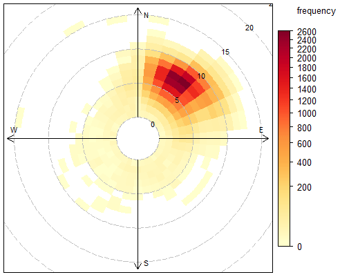
Figure 1 The frequency of hourly averaged wind speed and direction from January 2014 to August 2019. Each square symbolizes 10^∘ of wind direction and 1 m s⁻¹ wind speed. Each dashed circle shows an increase in wind speed of 5 m s⁻¹.

2.2 Measurement technique

NO_x has been measured at the CVAO since 2006 using a NO_x chemiluminescence instrument manufactured by Air Quality Design Inc. (AQD), USA. The chemiluminescence technique involves the oxidation of NO by excess O₃ to excited NO₂ (Reaction R9) (Clough and Thrush, 1967; Clyne et al., 1964; Fontijn et al., 1970). The excited NO₂ molecules can be deactivated by emitting photons (Reaction R10) or by being quenched by other molecules (Reaction R11), such as N₂, O₂, and in particular H₂O. The emitted photons are detected by a photomultiplier tube detector (PMT), which gives a signal that is linearly proportional to the mixing ratio of NO sampled. The measurement of NO_x and NO₂ requires photolytic conversion of NO₂ to NO (Reaction R3) followed by NO chemiluminescence detection (Kley and McFarland, 1980).

$$\begin{array}{}\text{(R9)}& {\displaystyle }\mathrm{NO}+{\mathrm{O}}_{\mathrm{3}}\to {\mathrm{NO}}_{\mathrm{2}}^{*}+{\mathrm{O}}_{\mathrm{2}}\text{(R10)}& {\displaystyle }{\mathrm{NO}}_{\mathrm{2}}^{*}\to {\mathrm{NO}}_{\mathrm{2}}+h\mathit{\nu }(h\mathit{\nu }>\mathrm{600}\mathrm{nm})\text{(R11)}& {\displaystyle }{\mathrm{NO}}_{\mathrm{2}}^{*}+\mathrm{M}\to {\mathrm{NO}}_{\mathrm{2}}\text{(R3)}& {\displaystyle }{\mathrm{NO}}_{\mathrm{2}}+h\mathit{\nu }\to \mathrm{NO}+\mathrm{O}{(}^{\mathrm{3}}\mathrm{P})(h\mathit{\nu }\le \mathrm{410}\mathrm{nm})\end{array}$$

Further details of the technique are documented in (Carpenter et al., 2010; Drummond et al., 1985; Fontijn et al., 1970; Lee et al., 2009; Peterson and Honrath, 1999; Reed et al., 2017; Val Martin et al., 2006).

2.3 Instrument setup

Ambient air is sampled from a downward-facing inlet placed into the prevailing wind with a fitted hood 10 m above the ground. A centrifugal pump at a flow rate of ∼ 750 L min⁻¹ pulls the air into a 40 mm glass manifold, resulting in a linear sample flow of 10 m s⁻¹, giving a residence time to the inlet of the NO_x instrument of 2.3 s. To reduce the humidity and aerosol concentration in the sampled air, dead-end traps are placed at the lowest point of the manifold inside and outside the laboratory. A Nafion dryer (PD-50T-12-MKR, Permapure) is used to additionally dry the sampled air, using a constant sheath flow of zero air (PAG 003, Eco Physics AG) that has been filtered through a Sofnofil (Molecular Products) and activated charcoal (Sigma Aldrich) trap (dew point −15 ^∘C). The air is sampled perpendicular to the manifold through a 47 mm PTFE (polytetrafluoroethylene) filter with a pore size of 1.2 µm.

Figure 2 Flow diagram of the NO_x instrument at the CVAO.

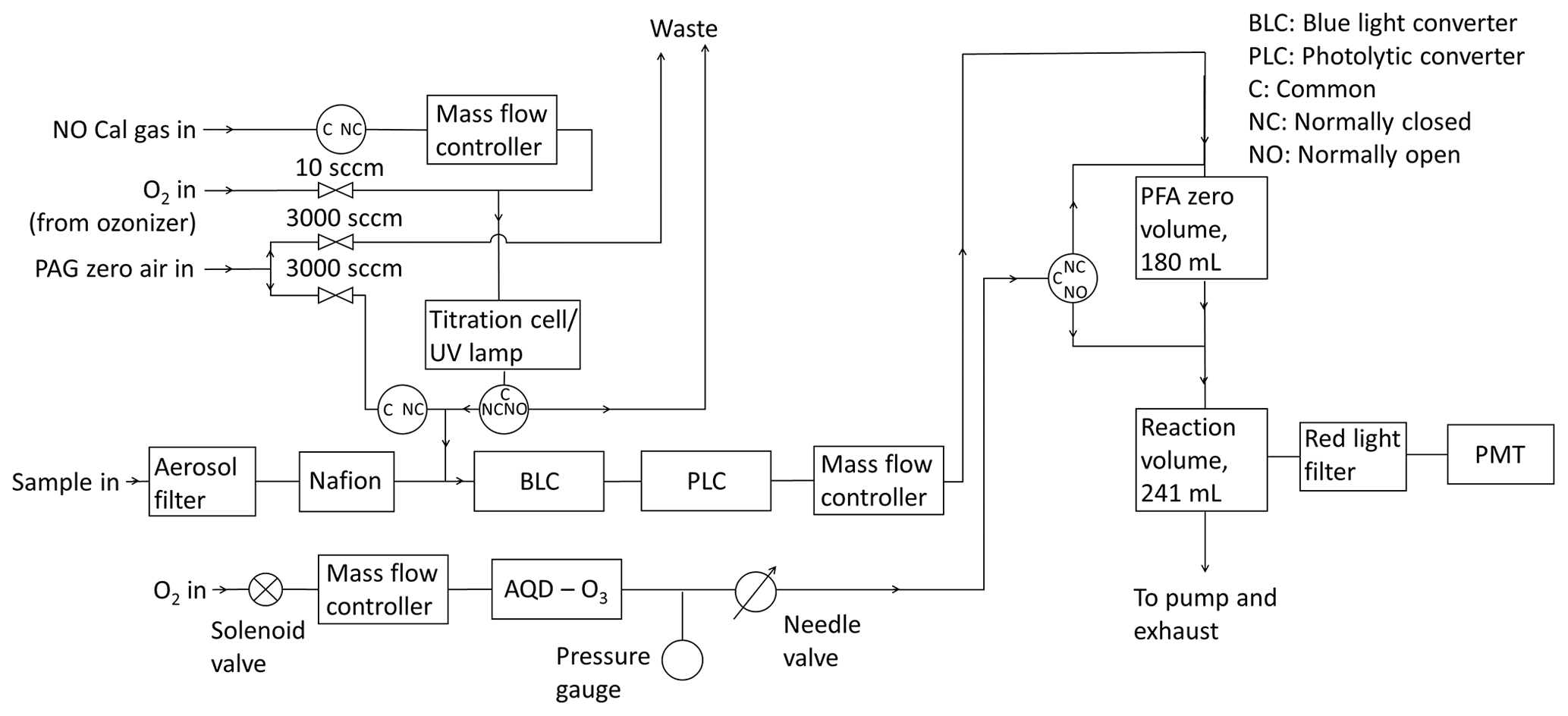
A schematic diagram of the instrument is shown in Fig. 2. Sampled air is passed through two different photolytic NO₂ converters, which are placed in series. The first is a commercial unit known as a BLC (blue light converter) supplied by Air Quality Design, as described in Buhr (2007). An ultraviolet light-emitting diode (UV-LED, 3 W, LED Engin, Inc.) array is placed in each end of a reaction chamber made of Teflon-like barium-doped material (BLC, λ = 385 nm, volume = 16 cm³). The entire block surrounding the reaction chamber is irradiated, giving the highest possible conversion efficiency of NO₂. Each array is cooled by a heat sink to maintain an approximately constant temperature inside of the converter when the diode arrays turn on. The second converter consists of two diodes (Hamamatsu Lightningcure L11921-500, λ = 385 nm) and a photolysis cell made of a quartz tube and two quartz windows glued to each end with a volume of 16 cm³ (PLC) following the design of Pollack et al. (2010). Aluminium foil is wrapped around the quartz tube to increase the reflectivity to give the highest conversion efficiency of NO₂. The diodes are placed at each end of the quartz tube, as shown in Fig. S2 in the Supplement, without touching the windows to avoid increases in the temperature when the diodes turn on. BLCs have been used at the CVAO since the instrument was installed in 2006, with the most recent converter installed in April 2015 (a BLC2 model), where the wavelength was changed to 385 nm from 395 nm. The PLC was installed in March 2017. The air flow through the instrument is controlled at ∼ 1000 sccm by a mass flow controller (MKS, M100B) giving a residence time of 0.96 s through each of the converters.

To measure NO and NO_x (NO + NO₂ converted into NO) the air is introduced to the chemiluminescent detector (CLD), where NO is oxidized by excess O₃ into excited NO₂ in the reaction volume (241 mL, aluminium with gold coating; Ridley and Grahek, 1990) shown in Fig. 2. The reaction volume is kept at low pressure to minimize quenching of excited NO₂ and thereby maximize the NO chemiluminescence lifetime. The photons emitted from the excited NO₂ molecules when they relax to ground state are detected by the PMT (Hamamatsu R2257P) to give a signal for NO. NO₂ is converted into NO by the BLC for 1 min, and then the PLC for 1 min, each period producing a signal due to NO + NO₂. The signal detected by the PMT (S_M) is caused by NO reacting with O₃ (S_NO), dark current from the thermionic emissions from the photocathode of the PMT (S_D), and an interference (S_I), which can be due to O₃–surface reactions that cause light emissions in the reaction cell, other reactions creating chemiluminescence, and from illumination of the chamber walls during NO₂ conversion (Drummond et al., 1985; Reed et al., 2016):

$$\begin{array}{}\text{(1)}& S_{\mathrm{M}}=S_{\mathrm{NO}}+S_{\mathrm{D}}+S_{\mathrm{I}}.\end{array}$$

The PMT is cooled to −30 ^∘C to reduce the dark current, giving the instrument a higher precision. Other molecules in the atmosphere such as alkenes also react with ozone and emit photons to reach their ground state but at a different timescale to that of NO₂ (Alam et al., 2020; Finlayson et al., 1974). This can give an interfering signal causing the NO and NO_x mixing ratios to be overestimated. However, most of these reactions emit photons at 400–600 nm and are therefore filtered by a red transmission cut-off filter (Schott RG-610) placed in front of the PMT (Alam et al., 2020). The filter transmits photons with a wavelength higher than 600 nm (Drummond et al., 1985). A background measurement is therefore required to account for the dark current of the PMT, O₃–surface reactions, and for the remaining interfering reactions occurring at a different timescale to that of NO₂. Background measurements are made by allowing ambient air to interact with O₃ in the zero volume (180 mL, PFA, Savillex, LLC) before reaching the reaction volume (Fig. 2). Most excited NO₂ molecules will reach their ground state before the sample reaches the PMT, meaning the signal from NO will not be measured. The efficiency of the reaction between NO and O₃ in the zero volume is calculated from the calibration, as explained in Sect. 2.4.3. Background measurements are performed every 5 min to take changing ambient conditions such as humidity into account, which can affect the background signal for example via the quantity of light emitted from interference reactions (S_I).

NO, NO₂, and the background signal are all detected on the same channel, and the instrument cycle is 1 min of background, 2 min of NO (when the NO₂ converters are off), 1 min of BLC NO_x (the BLC converter is on), and 1 min of PLC NO_x (the PLC is on).

2.4 Calibration

Prior to June 2019, calibrations were performed every 73 h by standard addition in order to account for temperature and humidity changes in the ambient matrix. In June 2019, the calibration frequency was changed to every 61 h to ensure that during any given month calibrations are carried out for approximately equal periods during the night and the day. To calibrate the NO sensitivity, 8 sccm of 5 ppm NO calibration gas in nitrogen is added to the ambient air flow of ∼ 1000 sccm, giving an NO mixing ratio of approximately 40 ppb. The mixing ratio used for calibrations is approximately 10 000 times that of the ambient measurements; however, due to reduced cylinder stability for lower NO mixing ratios it is difficult to calibrate at much lower mixing ratios, and the chemiluminescence is expected to be linear across the range of expected mixing ratios (Drummond et al., 1985). The calibration gas is added between the PTFE filter and the NO₂ converter as shown in Fig. 2. The conversion efficiency of the BLC and the PLC is calibrated by gas phase titration (GPT), where oxygen is added to the sampled NO calibration gas before entering the titration cell, which contains a UV lamp that converts oxygen to ozone. Between 60 % and 80 % of the NO calibration gas is oxidized into NO₂, giving a known mixing ratio of NO₂. A theoretical calibration sequence is shown in Fig. 3. The first cycle is to calibrate the sensitivity and the second is to calibrate the NO₂ conversion efficiency. Each actual calibration includes three cycles of sensitivity calibration and two cycles of conversion efficiency calibration. The signal from NO₂ observed in the NO sensitivity calibration is due to traces of NO₂ in the calibration gas. Figure S3 shows the observed percentage of NO₂ in the calibration cylinders from January 2014 to August 2019 calculated from the measured sensitivity (Sect. 2.4.1) and the conversion efficiencies (CE) of the two converters (Sect. 2.4.2):

$$\begin{array}{}\text{(2)}& {\displaystyle }{\mathrm{NO}}_{\mathrm{2}}\text{in cylinder (ppt)}={\displaystyle \frac{\left({\mathrm{NO}.\mathrm{c}}_{\left(\mathrm{1}\right)}-{\mathrm{NO}}_{\left(\mathrm{1}\right)}\right)}{\text{Sensitivity}\times \text{CE}}},\text{(3)}& {\displaystyle }\text{Percentage }{\mathrm{NO}}_{\mathrm{2}}={\displaystyle \frac{{\mathrm{NO}}_{\mathrm{2}}\text{in cylinder}}{{\mathrm{NO}}_{\mathrm{2}}\text{in cylinder}+\mathrm{NO}\text{cal conc.}}}.\end{array}$$

The percentage is stable for both converters; however, the PLC shows approximately 3 %–4 % NO₂ in the NO calibration gas compared to 5 %–10 % for the BLC, which is caused by a BLC artefact. The cylinders used were certified to ≤ 2 % NO_2.

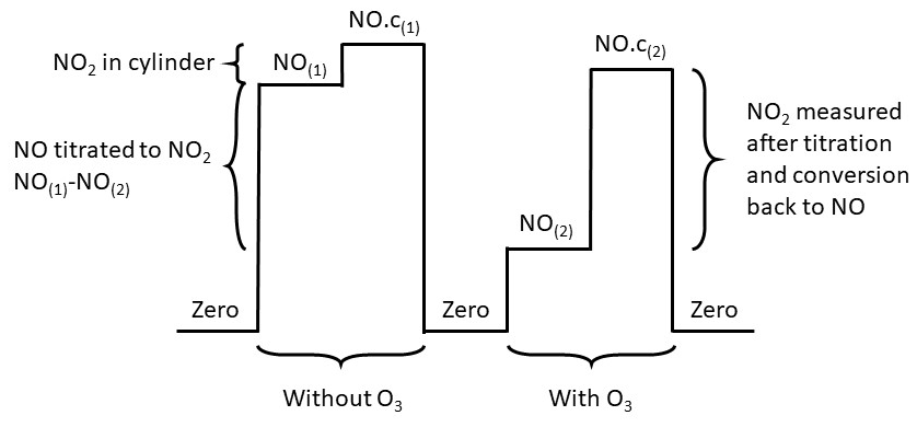
Figure 3 A theoretical calibration cycle. “NO” is the measurement of only NO, i.e. when the converters are off; “NO.c” is when one of the converters are on therefore the measurement is NO + NO₂; and (1) and (2) represent untitrated and titrated NO, respectively.

2.4.1 Sensitivity

The sensitivity of the instrument is calculated from the increase in counts per second caused by the calibration gas during NO calibration (untitrated, i.e. without O₃) and from the mixing ratio of the calibration gas as shown by Eq. (4). The NO counts per second from the previous measurement cycle before the calibration is subtracted to give the increase due to the calibration gas. The previous cycle needs to be stable and low in NO to give an accurate sensitivity, which is the case at the CVAO.

$$\begin{array}{}\text{(4)}& \text{Sensitivity}={\displaystyle \frac{\begin{array}{c}\mathrm{\text{Counts per second during calibration}}-\\ \mathrm{\text{Counts per second in previous cycle}}\end{array}}{\text{Mixing ratio of calibration gas}}}\end{array}$$

The sensitivity of the instrument depends on the pressure of the reaction chamber, the ozone mixing ratio in the reaction chamber, the flow of the sample through the reaction chamber, and the temperature of the reaction chamber. To maintain a stable sensitivity, all four parameters should be kept stable (Galbally, 2020). From January 2014 to August 2019, the sensitivity varied between 2.7 and 7.4 counts s⁻¹ ppt⁻¹ with changes of less than 5 % between subsequent calibrations (see Fig. S4), unless the instrument was turned off for a long period of time due to instrumental problems.

2.4.2 Conversion efficiencies

The conversion efficiency of the BLC and the PLC is calculated based on the titrated (with added O₃) and the untitrated (without added O₃) NO calibration gas, as described in Eq. (5). The numerator gives how much of the NO is titrated into NO₂, and the denominator represents the NO₂ measured when taking the NO₂ content in the NO calibration gas into account. In Eq. (5), “NO” is the measurement of only NO, i.e. when the converters are off; “NO.c” is when one of the converters are on and thus the measurement is NO + NO₂; and (1) and (2) represent untitrated and titrated NO, respectively.

$$\begin{array}{}\text{(5)}& \begin{array}{rl}\mathrm{CE}& ={\displaystyle \frac{\left[\left({\mathrm{NO}.\mathrm{c}}_{\left(\mathrm{2}\right)}-{\mathrm{NO}}_{\left(\mathrm{2}\right)}\right)-\left({\mathrm{NO}.\mathrm{c}}_{\left(\mathrm{1}\right)}-{\mathrm{NO}}_{\left(\mathrm{1}\right)}\right)\right]}{\left[{\mathrm{NO}}_{\left(\mathrm{1}\right)}-{\mathrm{NO}}_{\left(\mathrm{2}\right)}\right]}}\\ & =\mathrm{1}-{\displaystyle \frac{{\mathrm{NO}.\mathrm{c}}_{\left(\mathrm{1}\right)}-{\mathrm{NO}.\mathrm{c}}_{\left(\mathrm{2}\right)}}{{\mathrm{NO}}_{\left(\mathrm{1}\right)}-{\mathrm{NO}}_{\left(\mathrm{2}\right)}}}\end{array}\end{array}$$

The conversion efficiency of the BLC has varied from 82 % to 91 % between its installation in April 2015 and August 2019 (j ∼ 3 s⁻¹). Prior to April 2015, an older-generation BLC (λ = 395 nm) with a conversion efficiency of 30 %–35 % was used (j ∼ 0.5 s⁻¹). The conversion efficiency of the PLC has varied between 50 % and 55 % from its installation in March 2017 to August 2019 (j ∼ 1 s⁻¹). See Fig. S5 for all the calculated conversion efficiencies.

2.4.3 Efficiency of the zero volume

Background measurements are made by reacting NO and interference compounds with O₃ in the zero volume (Fig. 2). The system is set up so that NO₂ produced from NO will relax to the ground state before it is measured in the downstream reaction chamber, whereas it is assumed that any interfering compounds will emit photons when reaching the reaction chamber and be measured as a background signal (Drummond et al., 1985; Galbally, 2020). If the zero volume is too small or the O₃ mixing ratio is too low, some untitrated NO may lead to NO₂ chemiluminescence within the reaction chamber, and the background will be overestimated. On the other hand, if the zero volume is too large, some of the interfering compounds may have relaxed to their ground state before the reaction chamber and the background signal will be underestimated. The residence time of the zero volume is 10.8 s compared to 14.5 s for the reaction volume. The efficiency of the zero volume can be calculated from the calibration cycle. The difference in background counts from before a calibration cycle to during the calibration cycle shows how much of the added NO from the calibration cylinder does not react with O₃ in the zero volume. By dividing this difference by the signal due to NO during the NO measurement of the calibration cycle, which is obtained by subtracting the NO measurement from the previous measurement cycle, the inefficiency of the zero volume is obtained. The efficiency is determined for each calibration cycle (Eq. 6) and plotted in Fig. S6. It is consistently above 98 %.

$$\begin{array}{}\text{(6)}& {\mathrm{Efficiency}}_{\mathrm{ZV}}=\mathrm{1}-{\displaystyle \frac{\text{cal zero}-\text{measurement zero}}{\text{NO cal}-\text{previous NO cycle}}}\end{array}$$

2.4.4 Artefact measurements

As described in Sect. 2.3, NO_x measurements may have artefacts from chemiluminescence caused by interfering gas-phase reactions and/or from compounds produced by illumination of the reaction chamber walls and pressure differences in the instrument (Drummond et al., 1985; Reed et al., 2016). To estimate artefacts, it is necessary to measure the signal from NO_x-free air. The calibration sequence is followed by sampling NO_x-free air generated from a pure air generator (PAG 003, Eco Physics AG) for 30 min. According to the manufacturer, the PAG not only scrubs NO, NO₂, and NO_y from the ambient air but also removes SO₂, VOCs, H₂O, and O₃. An overflow of PAG air is introduced between the aerosol filter and the NO₂ converters as shown in Fig. 2 and the cycle of background, NO, NO_x BLC, and NO_x PLC is used to estimate artefact NO and NO₂ measured by the instrument. The artefacts are estimated using the sensitivity and conversion efficiencies measured in ambient air, where humidity is expected to be higher. This could cause the artefacts to be either underestimated or overestimated.

NO artefact

The NO artefact can be caused by two things: alkenes reacting with O₃ and giving chemiluminescence above 600 nm at approximately the same rate as NO₂ or a difference in pressure between the zero volume and the reaction volume. An artefact caused by alkenes will be positive and overestimate the NO mixing ratio, where an artefact due to a pressure difference can be either negative or positive. It can be estimated as the offset from 0 ppt when the mixing ratio sampled is 0 ppt. The NO mixing ratio is expected to be 0 ppt when sampling NO_x-free air or between 22:00 and 04:00 UTC at night. NO generated during the day is rapidly oxidized into NO₂ through reactions with O₃ and RO₂ after sunset. During the night, NO is not generated from photolysis of NO₂, and there are no significant local sources of NO at Cabo Verde when the air masses come from over the ocean (which is > 95 % of the time). The average NO mixing ratio between 22:00 and 04:00 UTC and the average NO mixing ratio from the PAG zero air tend to be very similar, with the PAG artefact (−3.7 ± 22.9 ppt, 2σ; January 2014–August 2019) being generally lower than the night-time artefact (0.4 ± 11.9 ppt, 2σ; January 2014–August 2019). Time series of both NO artefact measurements can be found in Fig. S7 in the Supplement. The night-time NO artefact is used as it is measured more frequently, as it contains the same ambient matrix with nothing scrubbed, and to eliminate the possibility of residual NO influencing background measurements determined from the PAG. Since the PAG scrubs VOCs it will also not give an estimate of the artefacts caused by fast-reacting alkenes.

NO₂ artefact

NO₂ converters have previously been shown to have artefacts caused by thermal or photolytic conversion of reactive nitrogen compounds (NO_z) other than NO₂ and illumination of the chamber walls (Drummond et al., 1985; Reed et al., 2016; Ryerson et al., 2000). Fast-reacting alkenes, which can cause overestimations of the NO mixing ratios, will not cause the NO₂ mixing ratio to be overestimated, since the NO signal is subtracted from the NO₂ signal.

The spectral output of an NO₂ converter with a wavelength of 385 nm was compared to absorption cross sections of NO₂ and potential interfering species such as BrONO₂, HONO, and NO₃ (Reed et al., 2016). The photolytic converter was shown to have good spectral overlap with the NO₂ cross section and minimal spectral overlap with other NO_z species, except for a small overlap with the absorption cross section of HONO. The interferences from BrONO₂, HONO, and NO₃ have additionally been evaluated previously for a similar setup using a Hg lamp (Ryerson et al., 2000). At equal concentrations of NO₂ and NO_z species, BrONO₂ and NO₃ were estimated to have a maximum interference of 5 % and 10 %, respectively, using a lamp with a wider spectral overlap with the interfering species than what is observed for the LEDs used at the CVAO (Ryerson et al., 2000). At the CVAO, HONO levels have previously been measured to peak at ∼ 3.5 ppt (at noon; Reed et al., 2017). For the typical Gaussian output of a UV-LED, this interference is calculated to be 2.0 %, 12.6 %, and 25.7 % for UV-LEDs with principle outputs of 395, 385, and 365 nm respectively, resulting in a maximum interference of < 0.5 ppt during peak daylight hours. Photolytic conversion of NO_z species is therefore not expected to be an important contributor to the NO₂ artefact at the CVAO due to the narrow spectral output of the LEDs.

Each converter is only on for 1 min in a 5 min cycle. For thermal conversion to be a major contributor to the artefact, the converter would have to increase in temperature during that 1 min and not the rest of the cycle, otherwise an increase in signal should be constant since the air continues to flow through the converters when they are turned off. Thermal decomposition of NO_z species is therefore not expected to have an effect in a climate like the one in Cabo Verde, where the sample temperatures are similar to the ambient temperatures.

It has been shown that the walls of a BLC, made out of a porous Teflon-like doped block, become contaminated from the ambient air over time, and when the walls are illuminated reactions take place on the surface, causing an artefact (Reed et al., 2016; Ryerson et al., 2000). The BLC is similar to the one used by Reed et al. (2016) and it is therefore expected to have an artefact due to reactions taking place on the surface. The PLC is not expected to be contaminated in the same way as it does not have porous chamber walls. Ryerson et al. (2000) observed an increase in artefact over time when sampling ambient air for a similar PLC; however, this is not observed for the PLC in the very clean environment at the CVAO (0–10 ppt between August 2017 and August 2019; see below), and surface reactions are therefore expected to give a negligible artefact for the PLC.

The total artefact can be determined by measuring the NO₂ signal when the NO₂ mixing ratio is 0 ppt; however, it is virtually impossible to scrub all NO_x from the ambient air and nothing else. To estimate the NO₂ artefact, PAG zero air is measured using both converters. The PLC measures between 0–10 ppt compared to 10–60 ppt using the BLC. Since, as discussed above, the NO₂ artefact of the PLC is assumed to be negligible, the measurement of PAG zero air by the PLC is assumed to represent the remaining NO₂ in the zero air after scrubbing. If the PLC does have an artefact, then both NO₂ measurements will be overestimated by the amount of this artefact. The signal from the BLC when measuring PAG zero air is expected to be due to the illumination of the chamber walls in addition to the traces of NO₂ left in the zero air. The artefact due to wall reactions in the BLC can therefore be estimated by subtracting the signal measured by the PLC.

3 Data analysis

Time periods with known problems such as maintenance on the manifold, ozone leaks, and periods when the PMT has not reached < −28 ^∘C are not included in the data set. The mean and standard deviation of the zero (background), NO, NO₂ BLC, and PLC are determined for each 5 min measurement cycle. To avoid averaging over the time it takes the detector to change and stabilize between the different types of measurements, the last 50 s of the measurement cycle are used for the background, the last 110 s for the NO counts, and the last 30 s for the BLC NO_x and the PLC NO_x counts. Each cycle is filtered based on the percentage standard deviations and differences in counts between subsequent cycles. If the standard deviation or the difference in counts are outside the mean ± 2σ (see Table 1) calculated from a 5-year period between 2014 and 2019, the cycle is not used for further analysis. This removes noisy data and sharp spikes but keeps data with sustained increases lasting more than 5 min.

Table 1 Evaluation parameters of the measurements. When a measurement falls outside any of the intervals it will not be used for further data analysis. The mean ± xσ is calculated for 2014–2019 for the zero and NO measurements and 2017–2019 for both NO₂ measurements.

^a The percentage standard deviation for each measurement cycle is determined as the standard deviation of a cycle divided by the mean of the same cycle. ^b Extreme measurements are determined to be mixing ratios that are outside the hourly mean ± 4 standard deviations of the hourly mixing ratio. ^c Extreme differences between the hourly mean and median of the mixing ratios are determined to be differences outside the hourly mean ± 4 standard deviations of the differences between the mean and median.

To obtain the signals due to NO and NO₂, the interpolated zero and NO measurements are subtracted from the NO and NO_x measurements, respectively. They are converted to a mixing ratio by using the interpolated sensitivity and conversion efficiency as shown in Eqs. (7) and (8).

$$\begin{array}{}\text{(7)}& {\displaystyle }\begin{array}{rl}& \text{NO mixing ratio}=\\ & {\displaystyle \frac{\text{NO measurement}-\text{background measurement}}{\text{Sensitivity}}}\end{array}\text{(8)}& {\displaystyle }\begin{array}{rl}& {\mathrm{NO}}_{\mathrm{2}}\text{mixing ratio}=\\ & {\displaystyle \frac{{\mathrm{NO}}_x\text{measurement}-\text{NO measurement}}{\text{Sensitivity}\times \text{CE}}}\end{array}\end{array}$$

The NO and NO₂ BLC mixing ratios are corrected by subtracting the interpolated artefacts described in Sect. 2.4.4. If the difference between two subsequent NO artefact measurements vary by more than the mean ± 2σ of the differences in NO artefacts determined from January 2014 to August 2019 (0.0 ± 6.2 ppt), the measurements made between are not used for further analysis due to a potential step change between the determinations.

Hourly averages of all the measurements are determined. If data coverage during the hour is less than 50 %, the hour is flagged and discarded from the data analysis. The hourly NO_x (NO + NO₂ PLC) mixing ratios between June 2017 and August 2019 are plotted as a function of wind speed and direction in Fig. 4. It can be observed that the concentrations are enhanced at low wind speed and when the air crosses the island (from the southwest). Measurements made at a wind speed < 2 m s⁻¹ or from a wind direction 100-360^∘ are, therefore, flagged as suspected of local contamination and are not used in the analysis. Extreme mixing ratios outside the mean  ± 4σ of the 5-year period for NO and 2-year period for NO₂ are flagged as suspicious (see Table 1 for boundaries). Lastly, inconsistency in the measurements, such as differences outside the mean  ± 4σ between the mean and median of a measurement (see Table 1 for boundaries) and differences between the two NO₂ measurements, are flagged as suspicious (0.4  ± 32.2 ppt). The data remaining after these removals are 88 % of the original NO and NO₂ BLC data set and 83 % of the NO₂ PLC data set.

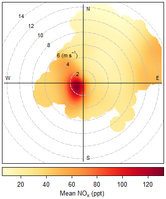
Figure 4 Total NO_x from June 2017 to August 2019 plotted as a function of wind speed and direction.

Corrections

As described above, excited NO₂ can be quenched by other sampled molecules, giving a lower observed mixing ratio than the real value. Water molecules are effective quenchers and therefore a correction is usually applied depending on the humidity (Matthews et al., 1977; Ridley et al., 1992). However, since the calibrations at the CVAO are performed by standard addition and a Nafion dryer is placed in front of the instrument, this is not necessary.

Additionally, NO can react with O₃ in the ambient air in the inlet and manifold giving an overestimation of NO₂ and an underestimation of NO. To correct for this the following equations are used (Gilge et al., 2014):

$$\begin{array}{}\text{(9)}& {\displaystyle }{\left[\mathrm{NO}\right]}_{\mathrm{0}}={\left[\mathrm{NO}\right]}_{\mathrm{E}\mathrm{1}}\times e^{k_{{\mathrm{O}}_{\mathrm{3}}}\times t_{\mathrm{E}\mathrm{1}}},\text{(10)}& {\displaystyle }\begin{array}{rl}& {\left[{\mathrm{NO}}_{\mathrm{2}}\right]}_{\mathrm{0}}=\left({\displaystyle \frac{J_{\mathrm{C}}+k_{{\mathrm{O}}_{\mathrm{3}}}}{J_{\mathrm{C}}}}\right)\\ & \times \left({\displaystyle \frac{{\left[\mathrm{NO}\right]}_{\mathrm{E}\mathrm{2}}-{\left[\mathrm{NO}\right]}_{\mathrm{E}\mathrm{1}}\times e^{-\left(k_{{\mathrm{O}}_{\mathrm{3}}}\times \left(t_{\mathrm{C}\mathrm{2}}-t_{\mathrm{C}\mathrm{1}}\right)+J_{\mathrm{C}}\times t_{\mathrm{C}\mathrm{2}}\right)}}{\mathrm{1}-e^{\left(-\left(k_{{\mathrm{O}}_{\mathrm{3}}}+J_{\mathrm{C}}\right)\times t_{\mathrm{C}\mathrm{2}}\right)}}}\right)\\ & -{\left[\mathrm{NO}\right]}_{\mathrm{0}},\end{array}\end{array}$$

where [NO]₀ is the corrected NO mixing ratio, [NO]_E1 is the uncorrected NO mixing ratio, [NO₂]₀ is the corrected NO₂ mixing ratio, [NO]_E2 is the uncorrected NO mixing ratio when the converter is on, $k_{{\mathrm{O}}_{\mathrm{3}}}$ is the rate of the reaction between NO and O₃ (k(O₃+NO) × [O₃] × 10⁻⁹ × M), t_E1 is the sum of the residence time from the inlet to entry of the converter and the time the air is in the converter, t_C1 and t_C2 are the time the air is in the converter when the converter is on and off, respectively, and J_C is the photolysis rate inside the converter. The residence time from the inlet to the entry of the converter has been 2.3 s since 2015, and the time the air is in each of the converters is 1.0 s (with and without the converter on). The O₃ mixing ratio measured at the CVAO varied between 5 and 60 ppb (with an uncertainty of 0.07 ppb) between 2014 and 2019. The ozone correction is calculated for each hour using a rate coefficient of 1.8 × 10⁻¹⁴ cm³ molecule⁻¹ s⁻¹ at 298K (Atkinson et al., 2004). This gives an average O₃ correction ±2σ of 6.8 ± 3.0 %, 1.7 ± 11.0 %, and 1.3 ± 7.1 % for NO, NO₂ BLC, and NO₂ PLC, respectively, when the mixing ratio measured is above 0.1 ppt (See Supplement for an example of the calculation). Thus, at the low mixing ratios of O₃ present at Cabo Verde and the short residence time for sampling, the corrections for O₃ are well within the noise of the measurements (see below) but are still included in the final calculated mixing ratios.

4 Uncertainty analysis

To be able to evaluate the NO_x measurements made at the CVAO an extensive uncertainty analysis is performed. A summary of the analysis can be found in Table 2, and a detailed description is given in the Supplement. The hourly precision and uncertainty of the instrument are estimated to characterize the uncertainties at the 95 % confidence interval (Bell, 2001). The hourly precision is estimated from the zero count variability, which is directly related to the photon-counting precision of the PMT. The uncertainty of the hourly measurements is estimated by combining all the uncertainties associated with the measurements. This includes uncertainties in the calibrations, artefact determinations, and O₃ corrections, as well as the precision of the instrument. The precision of the NO and NO₂ measurements are both included in the total uncertainty of the NO₂ measurements as the NO measurements are subtracted from the NO₂ measurements. Each term is converted into ppt to be able to combine them using error propagation.

Table 2 Calculated uncertainties associated with the NO_x measurements. The values in bold are the combined uncertainties for each type of measurement. Each uncertainty is given as the mean uncertainty ±2 standard deviations of the data between January 2014 and August 2019 for NO and from March 2017 to August 2019 for both NO₂ measurements.

^a The individual uncertainties associated with the calibration can be found in Table S1. ^b The individual uncertainties associated with the artefact determination can be found in Table S2.

The 2σ precision for hourly averaged NO data between January 2014 and August 2019 is 1.0 ± 0.9 ppt. The hourly precisions reported here are in good agreement with our previously reported 1σ precision of the instrument of 0.30 ppt (Reed et al., 2017) and the 2σ precision of 0.6–1.7 ppt (Lee et al., 2009). The NO₂ precisions are determined by taking the conversion efficiency of the respective converters into account. The hourly 2σ precision for hourly averaged NO₂ data between March 2017 and August 2019 becomes 1.5 ± 0.8 and 2.7 ± 2.2 ppt for the BLC and PLC, respectively. The determined NO₂ precisions are within the interval of previously reported precisions for the same instrument (Lee et al., 2009; Reed et al., 2017).

Figure 5 Panel (a) shows the time series for filtered O₃-corrected NO from 1 August 2017 to 31 July 2018. Panels (b), (c), and (d) zoom in on October 2017, December 2017, and April 2018, respectively. Panels (e), (f), and (g) show the average diurnal of NO for October 2017, December 2017, and April 2018, respectively, with the coloured areas being ±2 standard errors. If there are fewer than 15 measurements available for the hour, it is not included in the diurnal.

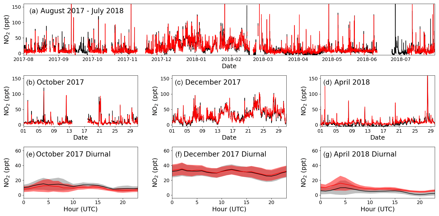
Figure 6 Panel (a) shows the time series of filtered O₃-corrected NO₂ from 1 August 2017 to 31 July 2018 for the BLC (black) and PLC (red). Panels (b), (c), and (d) zoom in on October 2017, December 2017, and April 2018, respectively, with the red line being the PLC and the black line the BLC. Panels (e), (f), and (g) show the average diurnal of NO₂ for October 2017, December 2017, and April 2018, respectively, with the red line being the PLC, the black line being the BLC, and the coloured areas being ±2 standard errors. If there are fewer than 15 measurements available for the hour, it is not included in the diurnal.

The total hourly uncertainty for each of the three measurements are determined by combining all the uncertainties described using propagation of uncertainties. The precisions are already calculated as hourly precisions in ppt. The calibration uncertainties are interpolated between each calibration and multiplied by the hourly mixing ratios of NO and NO₂ to calculate hourly uncertainties in ppt. The artefact uncertainties are interpolated between each artefact determination, and the uncertainty due to ozone corrections is determined by multiplying the percentage uncertainties by the hourly mixing ratios of NO and NO₂. The hourly uncertainties are determined to be 1.4 ± 1.5, 8.4 ± 7.5, and 4.4 ± 5.8 ppt for NO, NO₂ BLC, and NO₂ PLC, respectively.

5 Results: examples of data

The first year of data (1 August 2017 to 31 July 2018) is chosen as an example of the resulting NO and NO₂ data sets. October 2017, December 2017, and April 2018 are used to highlight the seasonality in the mixing ratios observed during a year of measurements. Figures 5a and 6a show the full O₃-corrected time series for NO and NO₂, respectively. Figures 5b–d and 6b–d show the time series for the 3 chosen months, and Figs. 5e–g and 6e–g show the 3 h rolling average diurnals for the same months. Monthly diurnals for NO and NO₂ for the entire year can be found in Figs. S9 and S10, respectively.

Figure 7 The BLC NO₂ mixing ratio is plotted against the PLC NO₂ mixing ratio. The dashed black line shows the one-to-one relationship. The red line is the linear least-squares regression of the hourly data with uncertainty in the y axis, and the blue line is the orthogonal distance regression with uncertainties in both the x and y axes.

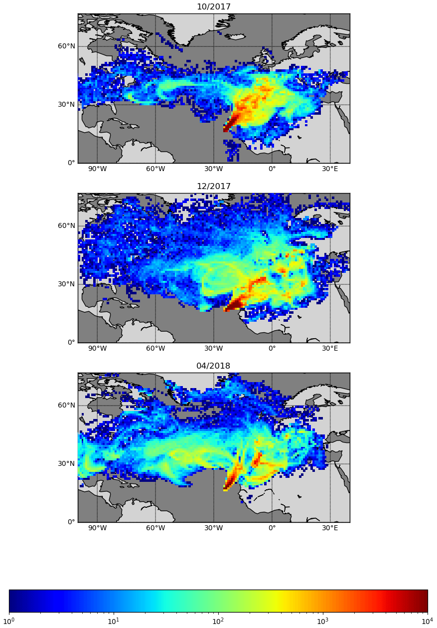
Figure 8 Back trajectories estimated for October 2017, December 2017, and April 2018. FLEXPART version 10.4 is used in backwards mode, driven by pressure level data from Global Forecast System (GFS) reanalyses at 0.5^∘ × 0.5^∘ resolution (Pisso et al., 2019; Stohl et al., 1998). The 10 d back-trajectory simulations are initialized every 6 h, releasing 1000 particles from the CVAO site.

Figure 9 Panel (a) shows the time series for total NO_x (NO + NO₂ PLC) from 1 August 2017 to 31 July 2018. Panels (b), (c), and (d) zoom in on October 2017, December 2017, and April 2018, respectively. Panels (e), (f), and (g) show the average diurnal of NO_x for October 2017, December 2017, and April 2018, respectively, with the coloured areas being ±2 standard errors. If there are fewer than 15 measurements available for the hour, it is not included in the diurnal.

Clear seasonality can be observed in the diurnal cycles of NO measurements with a maximum of ∼ 10 ppt in winter and a minimum of ∼ 2 ppt in the spring and summer. This is in good agreement with that reported for previous years (Lee et al., 2009; Reed et al., 2017). The two NO₂ measurements are in general in good agreement when looking at the time series in Fig. 6. Offsets of up to 10 ppt between the two measurements can be seen over some time periods (e.g. April, Fig. 6d), which are most likely caused by the calculated BLC artefact for those periods either being too high or too low. This is supported by the diurnals having the same shape but with an offset. Monthly diurnals of the two NO₂ measurements agree within 2 standard errors, except in August 2017, where the offset between the two measurements is larger than for the remaining months. NO₂ shows a fairly flat diurnal signal, although a small increase in daytime NO₂ is evident in some months, which is in agreement with that reported for previous years (Lee et al., 2009; Reed et al., 2017). Spikes in the early morning are noticeable in the NO₂ diurnals for July–November, which correspond to the months with an average lower wind speed than the rest of the year (the diurnal for April also shows a spike; however, it is caused by data from one morning). These spikes could be caused by local fishing boats passing upwind of the observatory in the morning hours, which will give a more prominent spike at low wind speed. Monthly wind speed diurnals can be found in Fig. S11. The good agreement between the two NO₂ measurements observed in Fig. 6 can also be observed in Fig. 7, where the two are plotted against each other. The data points are scattered around the 1 : 1 line shown in black. A linear least-squares regression (with uncertainty in the BLC measurements) and an orthogonal distance regression (ODR) (with uncertainty in both measurements) are performed to evaluate the scatter of the data points between August 2017 and 2019. The resulting regression lines are displayed in red (BLC = 0.99 × PLC + 0.7 ppt) and blue (BLC = 1.08 × PLC − 0.6 ppt). The deviation in the slope from 1 for both regressions are consistent with the uncertainty in the measured NO₂ artefact, which has been determined to be 7.2 ± 7.2 ppt.

The seasonality of the NO measurements can be explained by a combination of the variation of the origin of the air masses arriving at the CVAO, meteorology, photolysis rates, and seasonality of emissions. Back trajectories of the 3 months used as examples are shown in Fig. 8. FLEXPART version 10.4 is used in backwards mode, driven by pressure level data from Global Forecast System (GFS) reanalyses at 0.5^∘ × 0.5^∘ resolution (Pisso et al., 2019; Stohl et al., 1998). The 10 d back-trajectory simulations are initialized every 6 h, releasing 1000 particles from the CVAO site. Further information on FLEXPART can be found in the Supplement. During the winter maximum (December) the back trajectories indicate that the air reaching CVAO is largely dominated by African air, compared to during the spring minimum (April), which is dominated by Atlantic marine air. Large West African cities such as Dakar and Nouakchott and/or the shipping lanes to the east–northeast of Cabo Verde are potential candidates for the source of elevated NO_x. The NO mixing ratios measured in October are higher than those in April and lower than in December. This may be due in part to the influence of polluted African air arriving at Cabo Verde, which is more prominent in October than in April but less so than in December. The NO₂ and the total NO_x (NO + PLC NO₂, Fig. 9) similarly show higher levels in December than April, but the mixing ratios observed in October are similar to those in April. It should be noted that some of the days with high percentages of African air have missing data or wind directions from other places than the northeast.

Table 3 NO, NO₂, and NO_x mixing ratios at different low NO_x sites.

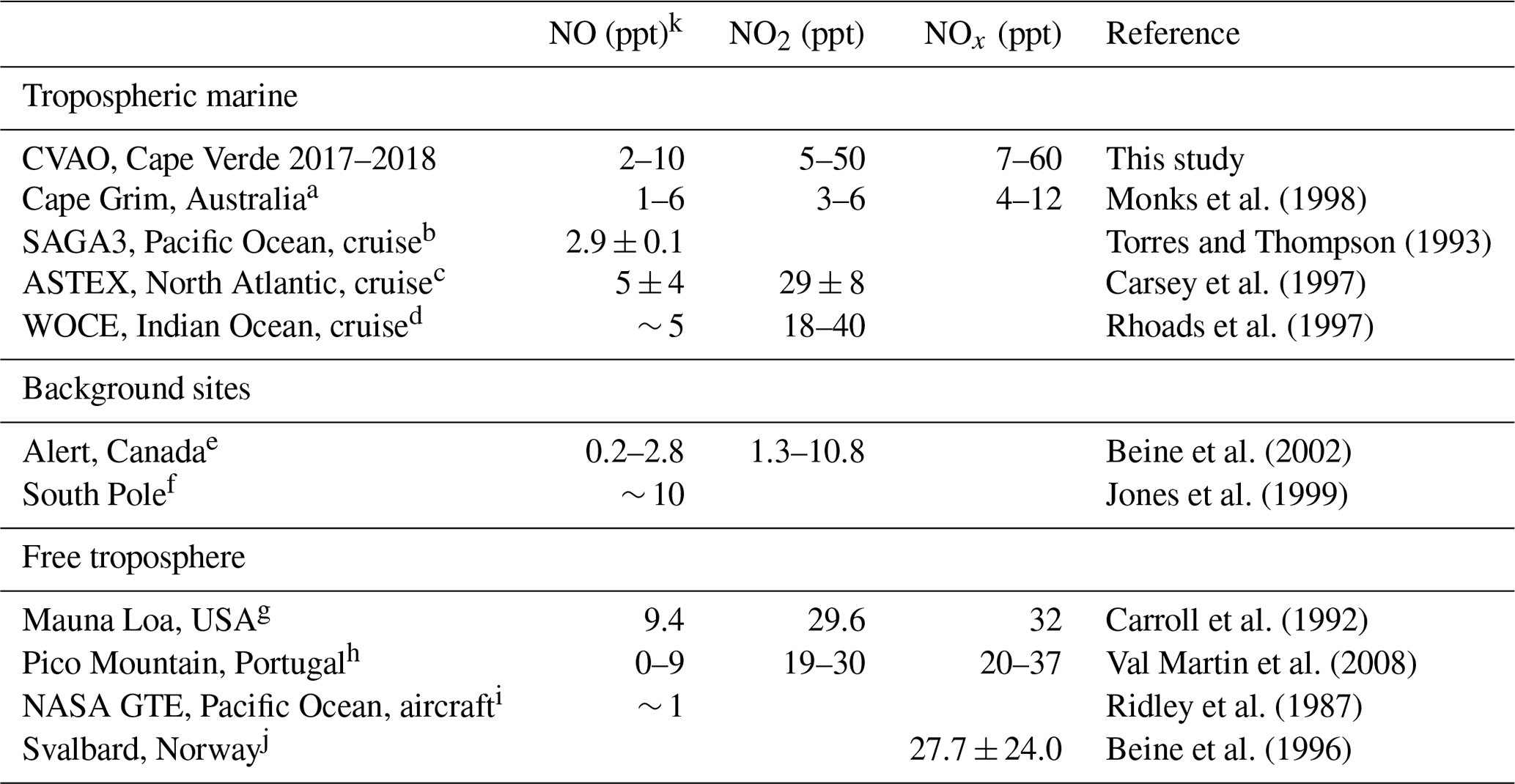
^a Measurements made during the SOAPEX (Southern Ocean Atmospheric Photochemistry EXperiment) campaign during austral summer in 1995. ^b Measurements from the Soviet-American Gases and Aerosols (SAGA) campaign between Hawaii and American Samoa between February and March. ^c Measurements from 6 clean days on the Atlantic Stratocumulus Transition Experiment (ASTEX). ^d Measurements from the World Ocean Circulation Experiment (WOCE) between South Africa and Sri Lanka. ^e Measurements made during 24 h darkness and in spring. ^f Measurements made from January–March 1997 at the German Antarctic research station, Neumayer. ^g Measurements made during the Mauna Loa Observatory Photochemistry Experiment (MLOPEX) in May 1988. ^h Measurements made at Mount Pico between July 2002 and August 2005. ⁱ Measurements made in the upper marine boundary layer from 13 flights between California and west of Hawaii. ^j Measurements made at the Ny-Ålesund Zeppelin mountain station on Svalbard during a spring campaign in 1994. ^k Daytime values.

From Table 3 it can be observed that the NO, NO₂, and NO_x measurements at the CVAO compare well to the few other measurements in the remote marine boundary layer as well as background sites in Alert, Canada, and measurements in the free troposphere. A wintertime seasonal increase in NO, NO₂, and NO_x can be observed during December–February, which corresponds to the months when surface air masses arrive at Cabo Verde from western Africa (Carpenter et al., 2010; Lee et al., 2009).

6 Conclusion

NO₂ was measured at a remote marine site by photolytic conversion to NO followed by chemiluminescence detection, using two different methods for conversion. A photolytic NO₂ converter with external diodes and a quartz photolysis cell (PLC) have been installed at the Cape Verde Atmospheric Observatory, and the NO₂ measurements have been compared to those of the historical BLC used at the site, which has internal diodes and a reaction chamber made of Teflon-like barium-doped material. The two measurements show good agreement (BLC = 0.99 × PLC + 0.7 ppt, linear least-squares analysis) with small differences due to uncertainties in the estimations of the BLC NO₂ artefact. Even though the PLC has a lower conversion efficiency (CE = 52 ± 4 %) than the BLC (CE = 85 ± 4 %), it is preferred due to its assumed negligible artefact as a consequence of having non-porous and non-reactive walls. The assumption of a zero artefact causes the hourly uncertainty of the NO₂ measurements to be roughly halved. With 2σ hourly precisions of 1.0 ± 0.9, 1.5 ± 0.8, and 2.7 ± 2.2 ppt and 2σ hourly uncertainties of 1.4 ± 1.5, 8.4 ± 7.5, and 4.4 ± 5.8 ppt for NO, NO₂ BLC, and NO₂ PLC, respectively, the instrument has a high repeatability and low uncertainties for all the measurements. The mixing ratios observed at the CVAO (NO: 2–10 ppt; NO₂: 5–50 ppt; and NO_x: 7–60 ppt at midday) are in good agreement with previous measurements at the CVAO as well as other remote measurements around the world.