the Creative Commons Attribution 4.0 License.
the Creative Commons Attribution 4.0 License.
 | 12 May 2021
Introducing hydrometeor orientation into all-sky microwave and submillimeter assimilation
Vasileios Barlakas
Alan J. Geer
Patrick Eriksson
Numerical weather prediction systems still employ many simplifications when assimilating microwave radiances under all-sky conditions (clear sky, cloudy, and precipitation). For example, the orientation of ice hydrometeors is ignored, along with the polarization that this causes. We present a simple approach for approximating hydrometeor orientation, requiring minor adaption of software and no additional calculation burden. The approach is introduced in the RTTOV (Radiative Transfer for TOVS) forward operator and tested in the Integrated Forecast System (IFS) of the European Centre for Medium-Range Weather Forecasts (ECMWF). For the first time within a data assimilation (DA) context, this represents the ice-induced brightness temperature differences between vertical (V) and horizontal (H) polarization – the polarization difference (PD). The discrepancies in PD between observations and simulations decrease by an order of magnitude at 166.5 GHz, with maximum reductions of 10–15 K. The error distributions, which were previously highly skewed and therefore problematic for DA, are now roughly symmetrical. The approach is based on rescaling the extinction in V and H channels, which is quantified by the polarization ratio ρ. Using dual-polarization observations from the Global Precipitation Mission microwave imager (GMI), suitable values for ρ were found to be 1.5 and 1.4 at 89.0 and 166.5 GHz, respectively. The scheme was used for all the conical scanners assimilated at ECMWF, with a broadly neutral impact on the forecast but with an increased physical consistency between instruments that employ different polarizations. This opens the way towards representing hydrometeor orientation for cross-track sounders and at frequencies above 183.0 GHz where the polarization can be even stronger.
- Article
(4473 KB) - Full-text XML
- BibTeX
- EndNote


Clouds containing ice hydrometeors are considered among the greatest ambiguities in both climate and numerical weather prediction (NWP) modeling systems (Duncan and Eriksson, 2018). Despite recent significant progress, their interaction with radiation has not been reliably assessed, in part owing to their high heterogeneity in shape and orientation within a cloud.
Over the last decades, several studies have explored the use of polarimetric observations at millimeter and submillimeter wavelengths to retrieve microphysical and macrophysical properties of ice hydrometeors (e.g., Czekala, 1998; Prigent et al., 2005; Xie, 2012; Defer et al., 2014). In particular (and also the focus of this study), oriented nonspherical ice hydrometeors are known to cause the observed brightness temperature (TB) differences between vertical (V) and horizontal (H) polarization. Here, this is denoted as the polarization difference (), owing to different scattering properties between V and H polarization (the dichroism effect; Davis et al., 2005). Evans and Stephens (1995a, b) simulated the sensitivity of polarized microwave (MW) frequencies (between 85.5 and 340.0 GHz) to nonspherical horizontally oriented ice hydrometeors. They reported a positive polarization signal, which increases with frequency. These findings were further supported by Czekala (1998): by conducting off-nadir simulations including polarization at 200.0 GHz, Czekala (1998) reported a PD of about 30 K linked to irregularly shaped horizontally oriented hydrometeors. Xie (2012) reported a PD of up to 10 K due to oriented snow observed by ground-based passive radiometry at 150.0 GHz. Studies involving active and passive satellite remote sensing instruments have further supported the presence of oriented ice hydrometeors (e.g., Prigent et al., 2001, 2005; Davis et al., 2005; Defer et al., 2014; Gong and Wu, 2017; Gong et al., 2020). Prigent et al. (2001, 2005) focused on passive MW imagers operating at low frequencies (37.0 and 85.0 GHz), i.e., the Tropical Rainfall Measuring Mission (TRMM) Microwave Imager (TMI) and the Special Sensor Microwave/Imager (SSM/I), and reported a PD due to horizontally oriented liquid at 37.0 GHz or ice hydrometeors at 85.0 GHz. At higher frequencies (up to 166.5 GHz), analogous PDs have been reported by Defer et al. (2014) and Gong and Wu (2017) derived from the Microwave Analysis and Detection of Rain and Atmospheric Structure (MADRAS) and the GPM (Global Precipitation Mission) microwave imager (GMI), respectively.
Defer et al. (2014) and Gong and Wu (2017) tried to interpret the observed PD in a conceptual way. Especially, Gong and Wu (2017) suggested an approximative modeling framework linking the observed PD to the ratio of optical thicknesses in V and H polarization (); this ratio is linked to the axial ratio of an oriented hydrometeor. This framework was tested on GMI observations at 89.0 and 166.5 GHz as well as on observations by the CoSSIR (Compact Scanning Submillimeter-wave Imaging Radiometer) airborne radiometer at a frequency of 640.0 GHz. The first rigorous simulations reproducing the observed PD were conducted by Brath et al. (2020). One of their main findings was the strong impact of the assumed shape of the ice hydrometeor on the simulated PD. Presently, GMI is the only operational instrument that measures ice hydrometeors including polarization. The upcoming Ice Cloud Imager (ICI) mission (Eriksson et al., 2020) will cover millimeter and submillimeter frequencies and will have channels measuring both V and H polarization at 243.2 and 664.4 GHz. This will provide further insights regarding the strong polarization signals from oriented ice hydrometeors. The observations from ICI will be assimilated under all-sky conditions for weather forecasting, further motivating the need to handle hydrometeor orientation.
All-sky radiance assimilation is the process of assimilating observations under the complete range of atmospheric conditions, i.e., clear sky, cloudy, and precipitation. Microwave humidity satellite observations in particular are gaining weight in forecasts, with the possibility to infer improved dynamical initial conditions (e.g., temperature, winds) from observations of cloud and precipitation (Geer et al., 2018). At the European Centre for Medium-Range Weather Forecasts (ECMWF), all-sky observations comprise around 20 % of the observation impact on forecasts (Geer et al., 2017). There is an ongoing effort to incorporate all possible observations that are sensitive to cloud and precipitation through the development of new capabilities, i.e., including visible, infrared, and submillimeter wavelengths (Geer et al., 2018).
The assimilation of satellite observations necessitates accurate and fast radiative transfer simulations. Currently, the leading radiative transfer models that are employed in global NWP systems for data assimilation (DA) are the Radiative Transfer model for TIROS Operational Vertical Sounder (RTTOV; Saunders et al., 2018) and the Community Radiative Transfer Model (CRTM; Liu and Boukabara, 2014). However, polarization due to the orientation of nonspherical hydrometeors is currently ignored. These forward models apply only “scalar” simulations; one calculation deals with either V or H polarization, although scattering by hydrometeors in nature transfers energy between polarizations. In addition, the models use the same ice scattering properties for both computations. It is currently too expensive to move to fully polarized radiative transfer in an assimilation system. However, this work will show that even with scalar radiative transfer, a significantly improved physical representation can be achieved by correctly varying the scattering properties as a function of polarization.
Following the work of Gong and Wu (2017), we explore the use of a simple scheme to approximate the effect of oriented ice hydrometeors in reproducing the observed PD from conical scanning MW imagers. In this study, special emphasis is placed on quantifying the best fit between the model and observations. The performance of such scheme is also tested in cycled DA experiments utilizing the Integrated Forecast System (IFS) from ECMWF. The ability to model oriented hydrometeors will provide essential information towards assimilating the observations from upcoming satellite missions, e.g., ICI and the Microwave Imager (MWI) that will fly on board the Meteorological Operational Satellite-Second Generation (MetOp-SG) operated by the European Organization of Meteorological Satellites (EUMETSAT). Reducing errors in forward modeling could improve the quality of the initial conditions for weather forecasting, as well as further improve weather forecasts.
2.1 Radiative transfer model
Radiative transfer simulations are conducted by means of RTTOV-SCATT (Bauer et al., 2006); this model accounts for multiple-scattering radiative transfer at MW and submillimeter frequencies and is part of the RTTOV package (Saunders et al., 2018). RTTOV-SCATT was developed by the EUMETSAT Numerical Weather Prediction Satellite Application Facility (NWP SAF) and is utilized by weather centers and scientists worldwide for fast modeling of all-sky radiances, as well as serving as the observations operator in the IFS at ECMWF.
RTTOV-SCATT employs the δ-Eddington approximation (Joseph et al., 1976) to solve the radiative transfer equation under all-sky conditions (clear, cloudy, and precipitating). The simulated TB is calculated as the weighted mean of the TB from two independent columns linked to clear-sky (TB,clear) and cloudy (TB,cloud) conditions:
where Cw is the effective cloud fraction representing the vertical mean of the cloud and precipitation fractions weighted by the hydrometeor content (Geer et al., 2009a, b). This is considered to be a fast approximation of sub-grid variability and, hence, the beam-filling effect (e.g., Barlakas and Eriksson, 2020).
The gaseous absorption component (e.g., oxygen and water vapor) is derived from precalculated regression tables supplied by the core RTTOV model (Saunders et al., 2018). Here, we employ version 12.3 (v12.3) of RTTOV-SCATT but with two main modifications on the path towards the final version 13 (v13.0) configuration. First, instead of a four-hydrometeor configuration (rain, snow, cloud liquid water, and cloud ice water), it separates convective snow (ice hydrometeors in deep convective cores, hereafter graupel) from large-scale snow (precipitating ice hydrometeors in stratiform clouds, hereafter snow), leading to a five-hydrometeor convention – a feature not available in v12.3. Further clarifications are given in Sect. 2.2. One of the main new aspects is the availability of a wider range of particle size distributions (PSDs) (e.g., McFarquhar and Heymsfield, 1997; Petty and Huang, 2011; Heymsfield et al., 2013) and the Atmospheric Radiative Transfer Simulator (ARTS) single-scattering database (Eriksson et al., 2018). This database is comprised of more realistic hydrometeor shapes (e.g., hail, graupel, and aggregates) covering a greater frequency range (1.0 to 886.4 GHz) compared with Liu (2008); hence, it is ideal for nonspherical hydrometeors, especially for the upcoming ICI mission. RTTOV-SCATT utilizes pre-calculated bulk optical properties (extinction, single-scattering albedo, and asymmetry parameter) for each hydrometeor (rain, snow, graupel, cloud liquid water, and cloud ice water), i.e., the hydrometeor tables. For each model level, the bulk properties are derived from the hydrometeor tables given the hydrometeor content and temperature. For details, the reader is referred to Geer and Baordo (2014).
Over ocean, surface emissivity is calculated by the FAST microwave Emissivity Model-6 (FASTEM-6, Kazumori and English, 2015). The land surface emissivity is primarily retrieved from satellite observations in surface-sensitive channels following the emissivity retrieval approach described in Karbou et al. (2010). This approach is based on the assumption that surface emissivity varies only slowly with frequency. Accordingly, surface emissivities are first retrieved in window channels at lower frequencies, and these values are then used as the surface emissivity for nearby sounding channels. This approach was extended to all-sky assimilation by Baordo and Geer (2016). However, the retrieval can be unreliable for strongly scattering scenes if the cloud and precipitation are inconsistent between the model and observations: it can generate a surface emissivity outside the physical bounds of zero and one, and even within those bounds, the retrieval must be further quality checked against values from an atlas. The atlas values are from the Tool to Estimate Land Surface Emissivities at Microwave (TELSEM) (Aires et al., 2011), which is a monthly average emissivity climatology constructed from 10 years of observations from the Special Sensor Microwave/Imager (SSM/I). If the emissivity retrieval is out of physical bounds or far from the value in the atlas, the atlas value is used instead.
2.2 Microphysical configuration
The microphysical setup employed in this study is found in Table 1. This setup was derived by Geer (2021, referred to in that paper as the “intermediate” configuration) using a multidimensional parameter search pertinent to ice hydrometeors, i.e., cloud overlap, convective water mixing ratio, PSD, and hydrometeor types for snow, graupel, and cloud ice. The configurations for rain and cloud water were not updated and follow the long-standing configurations for all-sky assimilation at ECMWF (Geer and Baordo, 2014). The search of the “optimal” microphysical setup was treated as a cost-minimization problem between actual observations and simulated observations from the Special Sensor Microwave Imager/Sounder (SSMIS). The analysis was conducted by means of latitude–longitude bins covering a frequency range of ≈19.0–190.0 GHz. The selection of the hydrometeor type was made on the basis of their bulk scattering properties, with the latitude–longitude binning enhancing the spatial differentiation between the three ice hydrometeor types, and the frequency range supporting the latter differentiation owing to the explicit spectral variation of the bulk properties. Each hydrometeor type is parameterized by different a and b coefficients that link the hydrometeor mass (m) to its size (maximum or geometric diameter; D), i.e., mass–size relation (). Accordingly, each hydrometeor leads to a distinct shape of the PSD (e.g., Eriksson et al., 2015) and, consequently, distinct bulk scattering “signature”. Although, the morphology of the selected hydrometeors may not be considered as the most physically correct representations, it is only the bulk scattering signature that needs to be correct in the context of DA.
Marshall and Palmer (1948)(Eriksson et al., 2018)Field et al. (2007)(Liu, 2008)Field et al. (2007)(see, Geer and Baordo, 2014)(Eriksson et al., 2018)Heymsfield et al. (2013)Table 1Microphysical setup for all the hydrometeors: PM denotes the particle model, PSD is the particle size distribution, CIW stands for cloud ice water, and CLW is the cloud liquid water. Dmin and Dmax denote the respective hydrometeor minimum and maximum sizes of the maximum diameter, and a and b comprise the coefficients of the mass–size relation that links the hydrometeor mass (m) to its size (maximum or geometric diameter; D), i.e., .
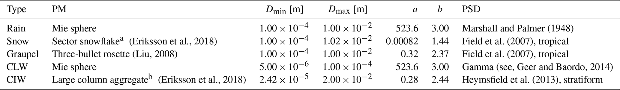
a In Eriksson et al. (2018), the minimum available size of the sector snowflake is m, but following Field et al. (2007), a m size cutoff has been applied.
b The large column aggregate is a mixture of two hydrometeors. Below a size of 3.68e−04 m, it is complemented with the long column single crystals (Eriksson et al., 2018) to provide a complete coverage in size. The name of the mixed hydrometeor follows the one comprising the majority range of size.
The search yielded the following microphysical representation (see Table 1), which was an update of a configuration found by Geer and Baordo (2014). The PSD introduced by Field et al. (2007) (the tropical configuration) was retained as a good representation for snow within the context of DA (e.g., Geer and Baordo, 2014; Fox, 2020) and was similarly found to be a good option to represent graupel in the IFS. Snow was previously represented by the sector snowflake by Liu (2008), but it was found that results could be improved with either the ARTS sector snowflake or the ARTS large plate aggregate. Note that the ARTS sector has near-identical single-scattering properties to the Liu (2008) representation, but it has less bulk scattering driven by a smaller a coefficient of the mass–size relation. The ARTS large plate aggregate, even though it is characterized by different single-scattering properties and mass–size relation, gives (for the chosen PSD) similar bulk scattering properties. This is an illustration of why the particle morphology is not yet fully constrained. The choice of the ARTS sector was on the basis that it gave a slightly better fit between observations from SSMIS and the equivalent simulated observations by the IFS. For the representation of graupel, similar considerations, particularly to achieve a bulk scattering signature with weak scattering at low frequencies (≈50.0 GHz) and strong scattering at high frequencies (≈190.0 GHz) led to the selection of the Liu three-bullet rosette. For cloud ice, the ARTS large column aggregate (LCA) is chosen to replace the physically unrealistic Mie sphere (Geer and Baordo, 2014). Here, the choice of PSD was the main issue, as most of the available PSDs (i.e., McFarquhar and Heymsfield, 1997; Field et al., 2007) were found to generate many large (centimeter in size) hydrometeors, inducing too much scattering at the highest frequencies considered and leading to rather large discrepancies between observations and simulations. Hence, the Heymsfield et al. (2013) PSD was chosen, as it generates fewer large-sized particles. Further, it is constructed on the basis of up-to-date aircraft observations of ice-containing clouds (stratiform configuration).
Note here that the polarized scattering correction scheme that is introduced later in Sect. 2.5 was used by Geer (2021) in order to derive a final and fully consistent microphysical configuration for RTTOV v13.0.
2.3 Assimilation system
The ECMWF forecasting system employs a semi-Lagrangian atmospheric model and a 12 h cycling four-dimensional (4D) variational DA (Rabier et al., 2000) in order to generate global analyses and 10 d forecasts. In this system, the direct assimilation of all-sky radiances from MW imagers went operational in 2009 and was subsequently extended to other sensors including microwave humidity sounders (Geer et al., 2017). Among the other data assimilated are in situ conventional measurements, radiances from polar-orbiting satellites (e.g., Advanced Microwave Sounding Unit-A, AMSU-A; Infrared Atmospheric Sounding Interferometer, IASI; and Advanced Technology Microwave Sounder, ATMS), geostationary radiances, satellite-derived atmospheric motion vectors, and surface winds from scatterometers. Note here that microwave imager observations are averaged (“superobbed”) in boxes of about 80 km × 80 km to meet the effective resolution in the model (Geer and Bauer, 2010).
The assimilation system is driven by the various observations via the background departure (d) (Geer and Baordo, 2014):
Here, yo and yb are the respective actual observations and the equivalent observations simulated from the background forecast:
The background atmospheric state, xb(t0), is a 12 h forecast from an earlier analysis, with t0 representing the start of the new assimilation window (Geer and Baordo, 2014). The nonlinear forecast model, M, propagates the atmospheric state from xb(t0) to the time of the observation, and the forward operator H (herein, RTTOV-SCATT) simulates the satellite-observed radiance from the model profile interpolated to the observation location. Finally, c denotes the bias correction term that accounts for systematic deviations between observations and simulations, which are modeled as a linear function of total column water vapor, surface wind speed, satellite scan angle, and other predictors; this is estimated as part of the DA process (Dee, 2004; Auligné et al., 2007).
The ECMWF assimilation model includes four prognostic hydrometeors, i.e., rain, snow, cloud water, and cloud ice, to represent the large-scale cloud processes, along with prognostic cloud and diagnostic precipitation fractions (Tiedtke, 1993; Forbes et al., 2011). Convective rain and snow are diagnostic variables, derived from a mass flux convection scheme that assumes that the convective cores occupy only 5 % of each grid box. When forming the input to RTTOV-SCATT, convective rain is added to the large-scale counterpart, but the convective snow is treated as a separate graupel hydrometeor type as explained above.
2.4 Observations
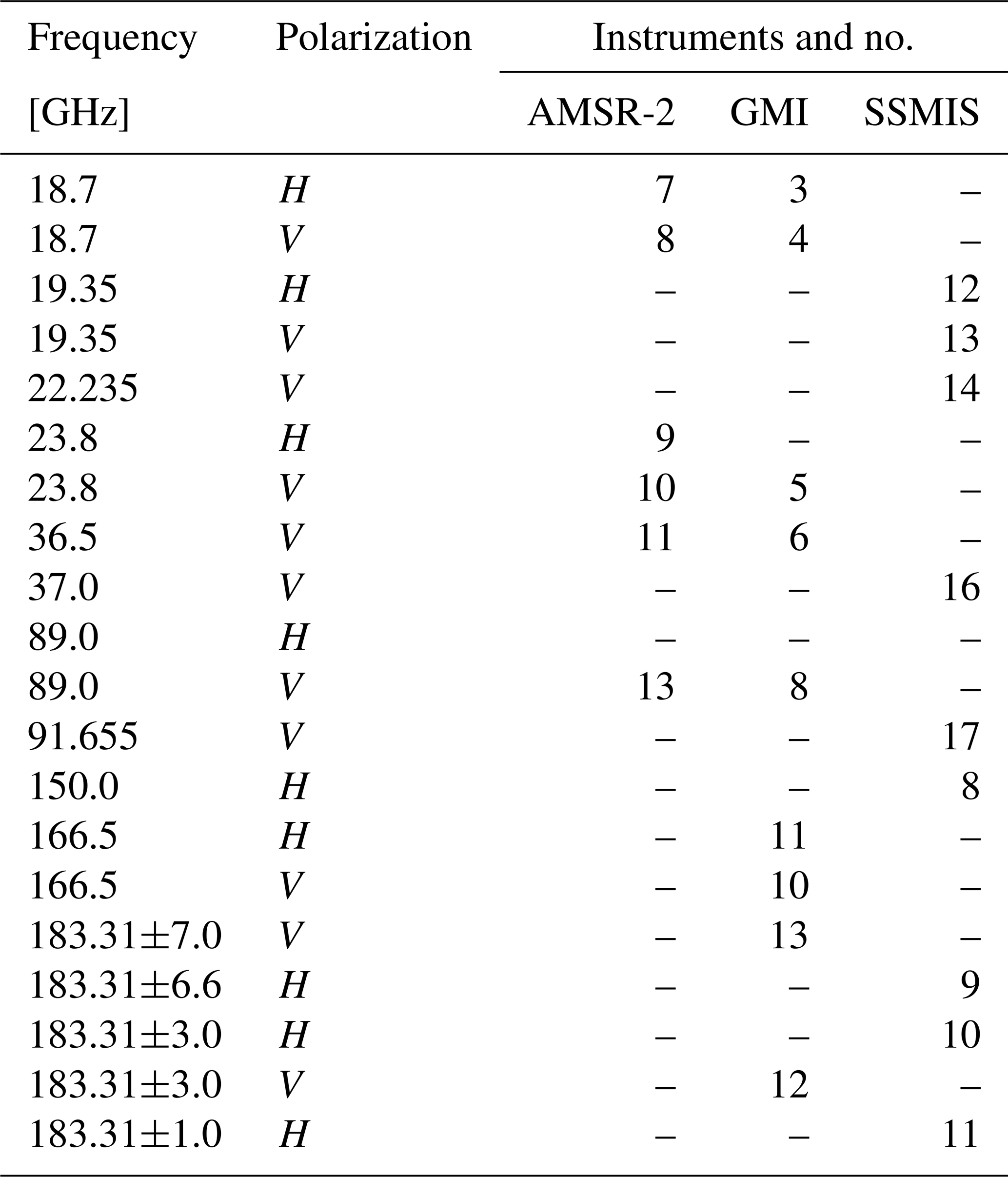
This study combines observations from GMI, the Advanced Microwave Scanning Radiometer-2 (AMSR-2), and SSMIS. Table 2 summarizes the channels of these instruments that are actively assimilated in the cycling DA experiments.
Table 2Channel characteristics of the Advanced Microwave Scanning Radiometer-2 (AMSR-2), Global Precipitation Mission microwave imager (GMI), and the Special Sensor Microwave Imager/Sounder (SSMIS) considered in this study.
2.4.1 Advanced Microwave Scanning Radiometer-2
The AMSR-2 is a conical scanning instrument with 16 channels ranging in frequency between 6.9 and 89.0 GHz, with dual-polarization capabilities. AMSR-2, flies on board the Japan Aerospace Exploration Agency (JAXA) Global Change Observation Mission – Water 1 (GCOM-W1) satellite and supplies global observations at a high spatial resolution and an Earth incident angle of 55∘ (Du et al., 2017).
2.4.2 Global Precipitation Mission microwave imager
The GPM core satellite carries a conical scanning MW radiometer, i.e., the GMI. It operates at frequencies between 10.65 and 190.31 GHz (13 channels overall) at a rather high spatial resolution, i.e., between ≈26 and ≈6 km, depending on the channel. The Earth incident angle is 52.8∘ for channels 1–9 and 49.1∘ for channels 10–13. GMI is the only operational passive instrument with dual-polarization channels at high frequencies, i.e., 166.5 GHz, offering unique capabilities in sounding ice hydrometeors, among others.
2.4.3 Special Sensor Microwave Imager/Sounder
The SSMIS is a conical MW instrument, with an Earth incident angle of 53.1∘, which is on board the Defense Meteorological Satellite Program F-17 spacecraft (Sun and Weng, 2012). It consists of 24 channels between ≈19.0 and ≈190.0 GHz (21 frequencies in total), three out of which are in both V and H polarization, i.e., 19.35, 37.0, and ≈91.65 GHz. Compared with AMSR-2 and GMI, SSMIS has a lower spatial resolution, with an instantaneous field of view ranging from ≈54 km (at the lowest-frequency channels) to ≈14 km (at the highest-frequency channels).
2.5 Polarized scattering correction
A widely used simplification in radiative transfer modeling is the assumption of totally randomly oriented (TRO) hydrometeors. Such hydrometeors are considered as macroscopically isotropic, meaning that there is no favored propagation direction or orientation and any induced polarization signal is only driven by the radiation scattered into the line of sight (e.g., see Barlakas, 2016). However, ice hydrometeors are characterized by nonspherical shapes and, thus, non-unit aspect ratios. This could potentially lead to preferential orientation driven by gravitational and aerodynamical forces (Khvorostyanov and Curry, 2014) or even by electrification processes (lightning activities in deep convective systems, Prigent et al., 2005). Under turbulence-free conditions, small nonspherical hydrometeors (diameters below ≈10 µm) are totally randomly oriented owing to Brownian motion (Klett, 1995); however, if they are large enough, they tend to be horizontally oriented as they fall depending on their shape: this holds true for thick plates with a diameter above ≈40 µm (Klett, 1995), whereas oblate spheroids and thin plates would adopt a horizontal orientation at sizes larger than ≈100 µm (Prigent et al., 2005, and references therein) and ≈150 µm (Noel and Sassen, 2005), respectively. However, turbulent effects can easily disrupt any orientation, especially for small hydrometeors, or introduce a wobbling motion around the horizontal plane at larger sizes (10–30 µm) (Klett, 1995). In addition, tumbling motions in strong turbulent conditions, e.g., within deep convective cores, induce total random orientation (Spencer et al., 1989).
Hydrometeor orientation results in anisotropic scattering with viewing-dependent optical properties, meaning different values of extinction at different polarization components of the incident radiation (the dichroism effect; Davis et al., 2005). Accordingly, in vector radiative transfer theory, the attenuation between the incident radiation and the hydrometeor is governed by a 4 × 4 extinction matrix K, depending on the incident direction and the orientation of the hydrometeor with respect to a reference system (e.g., Barlakas, 2016). This reference system (or, in other words, the laboratory system) is a three-dimensional Cartesian coordinate system that is characterized by a specified position in space and shares the same origin as the hydrometeor coordinate system; note that for typical applications, the z axis of the laboratory system would be aligned with the local vertical direction. Although the selection of the hydrometeor system is arbitrary, it is commonly specified by the shape of the hydrometeor (Mishchenko et al., 1999). In the case of an axial symmetry, for example, it is common to align the hydrometeor z axis along the direction of symmetry, with its largest dimension being aligned to the x–y plane (Brath et al., 2020). This acknowledges the tendency for hydrometeors to have horizontal alignment. Now, the orientation of the hydrometeor coordinate system, i.e., hydrometeor orientation, with respect to the laboratory system can be described by the three Euler rotation angles (rotations are applied in order): α∈ [0, 2π] around the laboratory z axis, β∈ [0, π] around the hydrometeor y axis, and γ∈ [0, 2π] around the hydrometeor z axis (see Fig. 1 in Brath et al., 2020).
In practice, scattering media consists of an ensemble of hydrometeors with various orientations. Thus, the single-scattering properties should be averaged over all possible orientations to derive the corresponding scattering properties of an ensemble of oriented hydrometeors (Mishchenko and Yurkin, 2017):
where f is a single-scattering property (e.g., extinction matrix) at a specific orientation, and p(α), p(β), and p(γ) describe the probability distributions of the three respective Euler angles.
In the case of TRO, all possible orientations are equally likely to occur, and p(α), p(β), and p(γ) describe uniform distributions. Consequently, the extinction matrix has no angular dependency, and it is reduced to its first element KTRO=K11, which describes the extinction cross section (Mishchenko and Yurkin, 2017; Brath et al., 2020). However, gravitational and/or aerodynamical forces can induce an axial symmetry, with the axis of symmetry specified by the direction of the force (Mishchenko et al., 1999). By aligning the laboratory z axis along the direction of the force, p(α) and p(γ) become uniform distributions resulting in an axial symmetry depending on β, i.e., tilt angle (Mishchenko et al., 1999). This results in the so-called azimuth random orientation (ARO), describing a preferred orientation to the horizon based on the tilt angle, with no favored orientation in the azimuth direction (Brath et al., 2020). In this case, K depends on the incident direction and the tilt angle, and it is reduced to only three independent elements (K11, K12, and K34). K12 represents the differences in the extinction between V and H polarization (cross section for linear polarization), whereas K34 describes the differences in the extinction between +45 and −45∘ polarization (cross section for circular polarization) and is not relevant here. For a comprehensive description of ARO, the reader is referred to Brath et al. (2020). Figure 1 highlights the differences in K between ARO and TRO for the large plate aggregate (LPA) at 166.9 GHz. It displays the first two elements of K normalized by the extinction at TRO as a function of the incident angle (θinc) for four tilt angles and two values of the size parameter x:
where Dveq is the volume-equivalent diameter of the hydrometeor, and λ is the wavelength. In the case of ARO, the scattering data of Brath et al. (2020) have been utilized. At the tilt angles considered here (0–60∘), hydrometeor orientation induces differences of up to 20 % of KARO,11 compared with KTRO. The maximum differences are reported at θinc of 0∘, whereas the smallest ones are found at around θinc of 55∘ and are in the range of ≈0–4 % (depending on x). In fact, for this incidence angle, the differences between KARO,11 and KTRO are close to zero over all sizes (not shown here). This implies that hydrometeor orientation does not change the overall level of extinction at Earth incident angles of around 55∘ (observation angle of conical scanners).
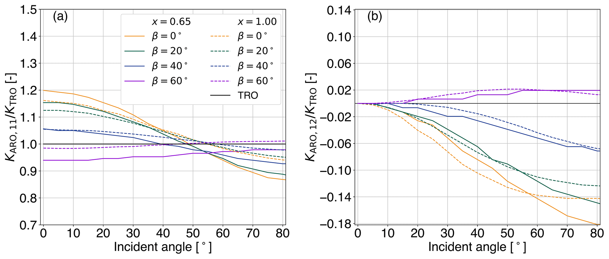
Figure 1For large plate aggregate, the extinction matrix elements of azimuth random orientation (ARO) normalized by the extinction cross section in the case of total random orientation (TRO) are shown as a function of incident angle θinc at 166.9 GHz. Results are presented for (a) and (b) for two size parameters (x=0.65, solid lines, and x=1.00, dashed lines) and four tilt angles (β) highlighted using different colors. The values for TRO are depicted in black.
At small θinc, the cross section for linear polarization (KARO,12) is close to zero, meaning that the differences in the extinction between V and H polarization are negligible. However, these differences increase with increasing θinc up to about ≈80∘. The largest differences in the extinction between V and H polarization (up to about 18 %) are derived for a tilt angle of 0∘. Recall here that results are presented for the LPA shape. For other shapes, e.g., plate type, the magnitude of KARO,12 is much larger (Brath et al., 2020). In any case, there are large differences in the cross section for linear polarization (K12) between ARO and TRO hydrometeors, even at Earth incident angles around 55∘. This (rather than any change in K11) is the likely explanation for the polarized scattering observed by microwave imagers.
To that end, a simple scheme has been implemented in RTTOV-SCATT to improve the physical representation of polarized scattering. To model the effect of ARO ice hydrometeors (snow, graupel, and cloud ice) in recreating the observed polarization signal from conical scanning radiometers, the layer optical thickness of TRO hydrometeors (τ) is increased in H-polarized channels and decreased in V-polarized channels by a correction factor α, leading to the following polarization ratio (ρ):
where τH and τV are the corrected optical thickness at H and V channels, respectively. This ratio can be seen as an indirect representation of the axial ratio of an oriented hydrometeor, and α approximates the differences in the extinction between the two channels (KARO,12; see Fig. 1b). In other words, α forces the extinction at V polarization (H polarization) to be weaker (stronger). Note here that the asymmetry parameter and the single-scattering albedo have been not modified, as it is not yet clear how to do so.
2.6 Experiments
Data assimilation experiments were conducted utilizing the 46r1 cycle of the IFS from ECMWF. This cycle was operational from June 2019 to June 2020. Compared with the operational system, the microphysical configuration of RTTOV-SCATT has been upgraded as described earlier, and a slightly reduced resolution of about 28 km (labeled Tco399) with 137 vertical levels has been used. Two types of experiments are considered:
-
To scrutinize the performance of the forward operator, a consistent sample of observations should be examined. Consequently, passive monitoring experiments were conducted to simulate GMI radiances. In the monitoring mode, the short-term forecast for all experiments is supplied from a single parent cycling DA experiment. In other words, the background forecasts (sometimes referred to as the first guess) come from the parent experiment, and changes to the usage of GMI observations do not feed back; the background atmospheric state is kept constant. Nine experiments were conducted for a period of 1 month (13 June to 13 July 2019), with ρ ranging from 1.1 to 1.5, with an increment of 0.05. Additional experiments were run in which the ρ was applied to each ice hydrometeor individually; for details, the reader is referred to Sect. 3.3.
-
To assess the potential long-term impact of ρ on the forecast, cycled DA experiments were run for a total period of 6 months, i.e., from 15 February to 31 May 2019 and from 13 June to 31 August 2019. Here, the improved forward operator is used for AMSR-2, GMI, and SSMIS as part of the DA process. The resulting analysis provides the initial conditions for the background forecast in the next cycle of DA. Hence, in contrast to the passive experiments, the background forecast and observational usage vary, and the changes can feed back over multiple cycles of DA. These experiments are described further in Sect. 3.4.
For the passive monitoring experiments, the period of 1 month was chosen on the basis that polarization signatures of oriented ice hydrometeors are fairly consistent through the seasons and across the globe (Gong and Wu, 2017; Galligani et al., 2021). For both types of experiments, to highlight whether the forward operator and the forecast are improved or degraded, control experiments were additionally run, with the improved physical representation of polarized scattering being turned off, meaning a ρ value of 1.0 (a correction factor of 0.0).
3.1 Overview
By means of passive monitoring experiments, the ability of ρ to simulate the observed polarization patterns due to oriented ice hydrometeors is explored. Accordingly, special emphasis is placed on the high-frequency dual-polarization channels of GMI (89.0 and especially on 166.5 GHz) because scattering due to ice hydrometeors (snow, graupel, and cloud ice) increases with frequency. For clarity, we discriminate between the observed (o) and simulated (background, b) polarization difference:
One of the challenges encountered was to screen out any surface contamination and, particularly, any strong polarization signal that originates from water surfaces (Meissner and Wentz, 2012); strongly polarized surfaces complicate the separation between cloudy and clear-sky conditions. Appendix A describes a number of careful screening checks that were used to minimize the surface contribution. Note here that, throughout Sect. 3, results are presented in terms of the screened data that are almost entirely free from surface contribution.
Figure 2 illustrates the global PD as a function of TBV at 166.5 GHz in the case of both observations and simulations. Polarized scattering from preferentially oriented ice hydrometeors leads to a PDo of up to 10–15 K (red) centered around 220 K, with increasingly low TBV indicating increasingly cloud-affected scenes. In fact, the arch-like shape of the PDo– (or ) relation appears to be universal (Gong and Wu, 2017). The existing modeling framework characterized by a polarization ratio of 1.0 (control run; green) completely fails to reproduce such polarization signal (see Fig. 2a). However, it provides valuable information regarding the surface contribution; if there was any simulated polarization signal due to ocean reflection, it would be visible. The remaining panels in Fig.2 (i.e., b–f) depict the ability of ρ to provide realistic simulations of this behavior, and a first glance indicates that a ρ value between 1.2 and 1.4 could do a reasonable job, as it is within the distributions of the observations.
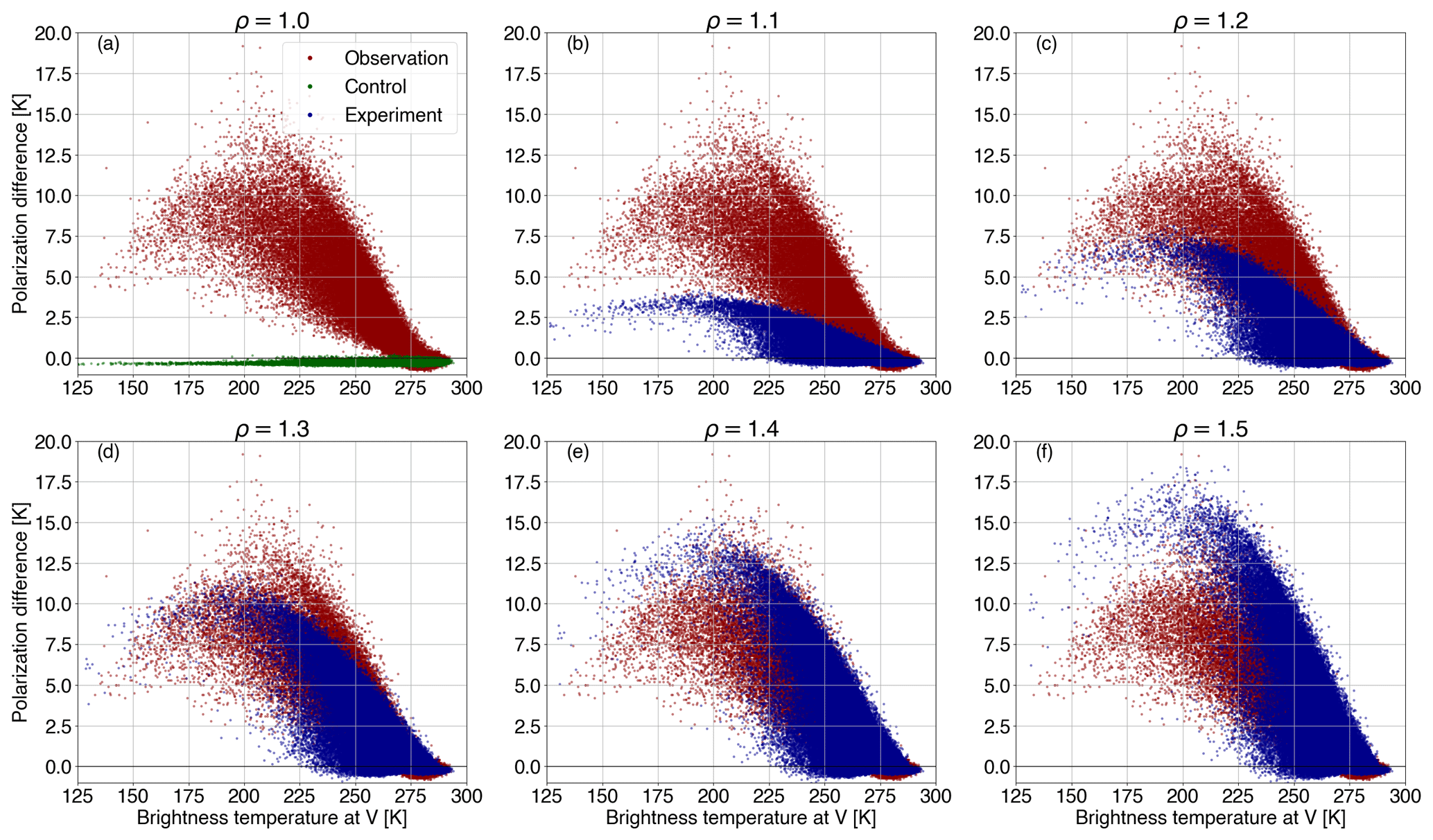
Figure 2Polarization difference between the vertically and horizontally polarized channels () as a function of TBV at 166.5 GHz as observed by GMI (PDo; red) and as simulated by the passive monitoring experiments (PDb; blue) for a period of 1 month (13 June to 13 July 2019). Results are presented for polarization ratios (ρ) ranging from 1.0 (control run; green) to 1.5, with a 0.1 increment.
3.2 Quantifying the fit of model to observations
In order to quantify the best fit between simulations and observations, the commonly used metrics are the mean, the standard deviation (σ), and/or the root mean square error (RMSE). Nonetheless, forecast modeling systems are still unable to predict cloud and precipitation at small scales; thus, they are characterized by mislocation errors that could lead to quite a large σ and/or RMSE (e.g., Geer and Baordo, 2014, and references therein). A more comprehensive assessment of the polarized scattering correction is achieved by measuring the divergence between the distributions of observations and simulations introduced in Geer and Baordo (2014):
where Pb and Po are the respective populations of simulations and observations in each bin, and “no. bins” denotes the total number of bins used in the comparison (which is a minor modification from the original approach). The metric of divergence describes how well the experiments approximate the observations by applying a penalty according to the logarithm base 10 of the ratio of the populations (φ; simulations divided by observations) in each bin. To avoid any infinite penalty in the case of zero populations, empty bins are replaced by a population of 0.1; varying this limit has a minor effect and increases or decreases the penalty effect. The complete set of statistics used here are the mean and skewness of PDo−PDb, the corresponding histogram divergence (i.e., one-dimensional (1D) divergence), and the two-dimensional (2D) divergence between the observed (PDo–) and simulated (PDb–) 2D histograms of the arch-like relationship, which are non-localized measures of the discrepancy between simulated and observed distributions.
Figure 3 depicts these statistical metrics with respect to the polarization ratio. Results are reported globally (black crosses), but the situations over ocean (blue triangles) and land (brown dots) are also described. Note here that the pixels across the coastline are excluded for ocean and land, whereas “global” represents the overall number of pixels (including the coastline). To begin with, the control run, which is highlighted by the corresponding green markers, is unable to provide realistic simulations of the observed PDs at both 89.0 (Fig. 3a–d) and 166.5 GHz (Fig. 3e–h); this leads to a mean error of about 1 K (globally), and the histograms (of PDo−PDb, not shown here) are described by right-skewed distributions that are more asymmetric over land compared to over the ocean (see skewness; Fig. 3b, f). At both frequencies, even a small increase to the polarization ratio above 1.0 reduces discrepancies (mean error; Fig. 3a, e) between observations and simulations and leads to a more symmetrical error (skewness; Fig. 3b, f); further increasing the polarization ratio additionally reduces both the mean and the skewness of PDo−PDb up to a point where the best ratio can be found. At 89.0 GHz and over the entire globe, the best polarization ratio is 1.5 (skewness is close to zero). However, over the ocean, a more symmetrical error is achieved by a smaller value (i.e., 1.45), but this could be attributed to the relatively low number of pixels that passed through the rather strict screening method that minimizes the strongly polarizing ocean surface. On the contrary, the dependency of the 166.5 GHz channel on the polarization ratio is characterized by similar behavior over both land and the ocean. An increase in ρ improves the representation of preferentially oriented ice hydrometeors up to a value of about 1.4 (in terms of the mean and the skewness); a further increase in ρ, increases PDo−PDb once again, although towards negative values. This implies that the corresponding histogram, from a right-skewed distribution, becomes symmetrical at a polarization ratio of 1.4 and turns into a left-skewed one at higher ρ values.
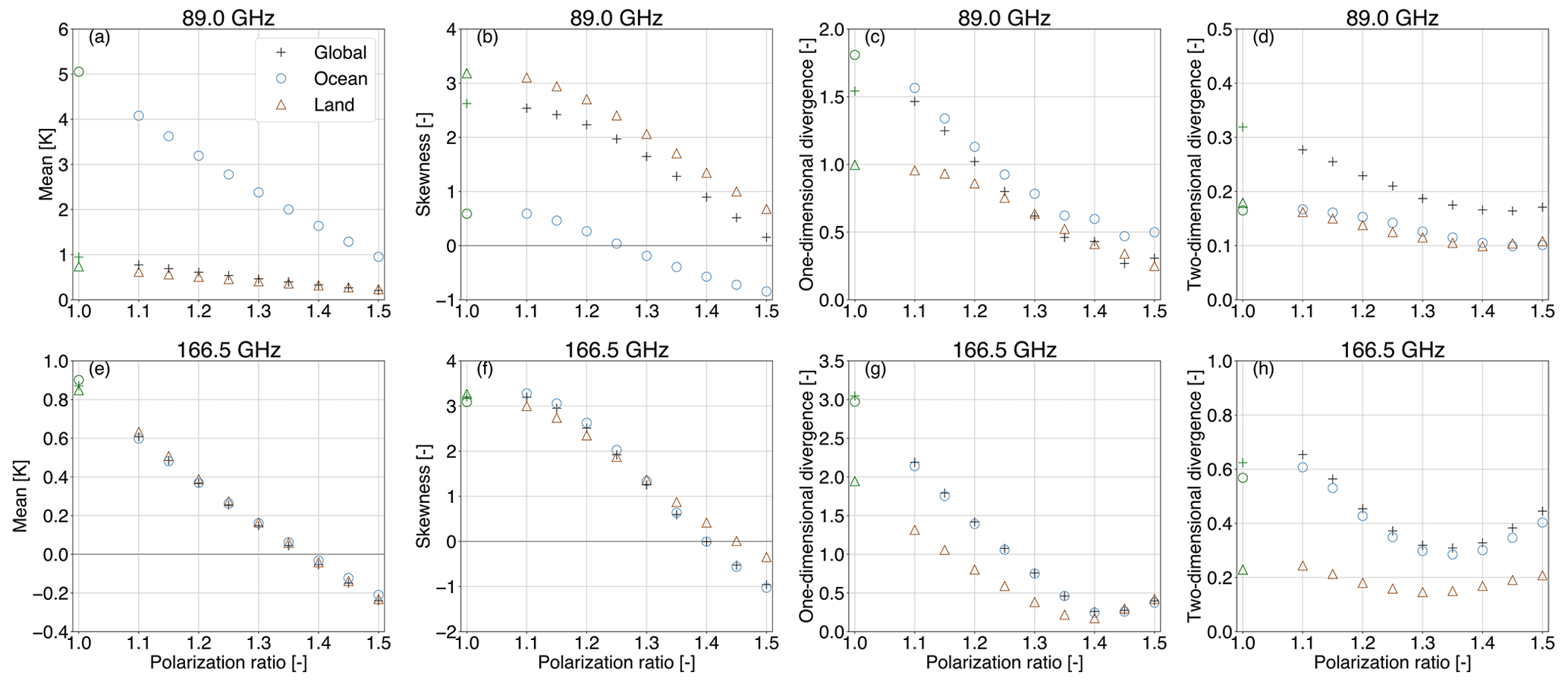
Figure 3Statistical metrics, i.e., mean, skewness, and one-dimensional (1D) divergence, describing the differences in polarization differences between observations and simulations, i.e., PDo−PDb, and the two-dimensional (2D) divergence between the observed (PDo–) and simulated (PDb–) 2D histograms of the arch-like relationship. Results are presented for 89.0 (a–d) and 166.5 GHz (e–h) over land (brown triangles), ocean (blue circles), and globally (black crosses) for a period of 1 month (13 June to 13 July 2019) as a function of the polarization ratio (ρ). In terms of the control run (ρ=1), the corresponding differences are highlighted in green.
In Fig. 3, the overall 1D and 2D divergence – Φ1D (Fig. 3c, g) and Φ2D (Fig. 3d, h), respectively – derived by Eq. (8) are also shown. At 166.5 GHz, the 1D divergence is in line with the conclusions drawn from the mean and skewness, whereas the corresponding 2D divergence marginally suggests that the minimum value is found at the lower polarization ratio of 1.35. At 89.0 GHz, both the 1D and 2D global divergence marginally pinpoint that the minimum value is acquired for the lower polarization ratio of 1.45, but results for present low sensitivity to the selected polarization ratio – especially in terms of the Φ2D. However, data assimilation assumes that errors are Gaussian and unbiased; hence, we prioritize minimizing the measure of skewness, rather than the 2D divergence.
To conclude, the polarization ratio that best models the orientation of nonspherical ice hydrometeors and leads to a more symmetrical error within the IFS is 1.5 for 89.0 GHz and 1.4 for 166.5 GHz. This is translated to increasing/decreasing τH (τV) by 20 % (a=0.2) at 89.0 GHz and by 16.7 % (a=0.167) at 166.5 GHz. Note here that there is low confidence in the optimal value of ρ obtained at 89.0 GHz; clarifications are given in Sect. 4.2. Consequently, the polarization ratio found at 166.5 GHz is chosen to further assess the impact of the polarized scheme on both the forward operator and the forecast impact.
Figure 4 provides an overview of the global performance of the polarization ratio of 1.4 to simulate the observed PDs at 166.5 GHz. To begin with, Fig. 4a illustrates the 2D histogram describing the observed arch-like relationship of PDo– introduced in Fig. 2 (red). Most of the points are bundled above ≈275 K and are linked to clear-sky conditions and PDs close to 0 K. The cloud-induced PDs are mostly accumulated at between ≈215 and ≈275 K. Figure 4b depicts the corresponding simulated PDb– relation for a ratio of 1.4, whereas Fig. 4c shows the 2D histogram divergence between PDo– and PDb– highlighting the performance of the selected ρ; note here that the 2D bin divergence denotes the lowercase letter “φ” (φ2D) in Eq. (8) and not the overall divergence which is represented by the capital letter “Φ” (Φ2D). One can see that such a ρ value offers quite a good approximation of the observed PDs (high slope where most of the points are accumulated), whereas it underperforms at values of brightness temperature below ≈225 K and at the lower part of the arch ( K) characterized by low PD values (0–2 K). For the situation at 89.0 GHz, the reader is referred to Fig. B1 in Appendix B.

Figure 4Two-dimensional (2D) histograms describing the arch-like relationship between the polarization difference and the brightness temperature at V polarization at 166.5 GHz as (a) observed (PDo–) by GMI, (b) simulated (PDb–) for a polarization ratio of 1.4, and (c) the 2D histogram divergence between PDo– and PDb–. In panel (c), white areas denote the case where both the observed and the simulated 2D bins are empty.
A 1D global comparison is found in Fig. 5. Firstly, Fig. 5a shows the histograms of the brightness temperature as observed (; red) by GMI and simulated () for a polarization ratio of 1.4 (blue) and 1.0 (green; control run). The solid and dashed lines denote TBV and TBH, respectively, and the shaded area highlights their difference. One can see that the IFS and RTTOV-SCATT underestimate the brightness temperature depressions linked to rather deep convective systems (at increasing low TB), but a polarization ratio of 1.4 realistically represents the histogram differences between TBV and TBH (blue shaded area), which is completely missed by the control run (limited green shaded area). Figure 5b illustrates the corresponding histograms of PDs. The control run (green) completely fails to reproduce any positive PDs larger than 0.2 K (see also Fig. 2a). On the other hand, a polarization ratio of 1.4 (blue) removes most of the discrepancies between observations and simulations. Figure 5c displays the related 1D divergence (φ1D) or, in other words, the logarithm base 10 of the ratio of the populations (see Eq. 8). The experiment with ρ=1.4 slightly overestimates the occurrences of PDs between 0.2 and about 5.0 K; thus, these occurrences are penalized with a positive logarithm base 10 ratio. From around 5.0 to 10.5 K, very good agreement is found between simulations and observations, whereas the largest differences are reported at negative and at the largest PD values (this ratio does not simulate PDs>15 K), leading to a total divergence (Φ1D) value of 0.260. In terms of the control run, any φ1D value corresponding to a PD above 0.2 K results from the penalty effect assigned to avoid infinite values. The control run yields a total divergence (Φ1D) value of 3.047.
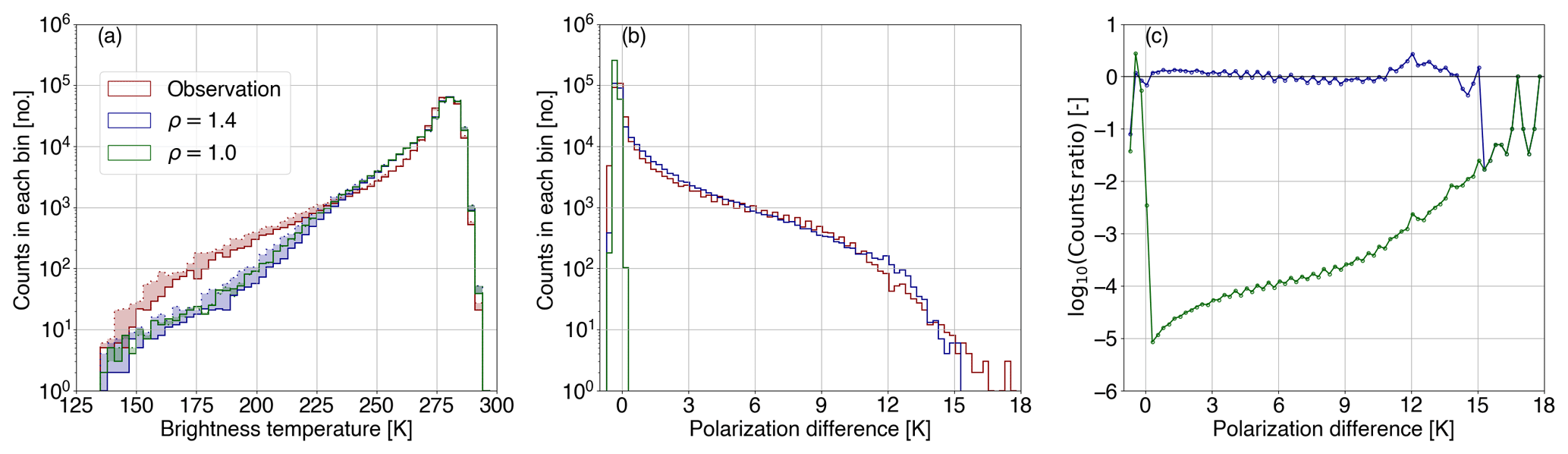
Figure 5(a) Histograms of the brightness temperature at 166.5 GHz as observed (; red) by GMI and simulated () for a polarization ratio of 1.4 (blue) and 1.0 (green; control run); solid and dashed lines denote the brightness temperature at vertical and horizontal polarization, respectively, and the shaded area highlights their difference. (b) Corresponding histograms of polarization differences (PD) and (c) the divergence between the distributions of PDo and PDb as a function of the polarization difference.
3.3 Polarization differences per hydrometeor type
To discriminate the polarization signal at 166.5 GHz induced by the various ice hydrometeors, additional passive monitoring experiments were conducted, whereby the polarization ratio of 1.4 was applied to snow, graupel, and cloud ice water individually. Figure 6 displays a global overview of the simulated PDb– arch-like relation compared to the observed one. Preferentially oriented large-scale snow produces most of the observed polarization signature, whereas deep convective snow (graupel) induces only low to medium PD values and a much lower peak (≈7.5 K). Interestingly, cloud ice produces a minor polarization signal, with negative values at increasingly cold TBV.
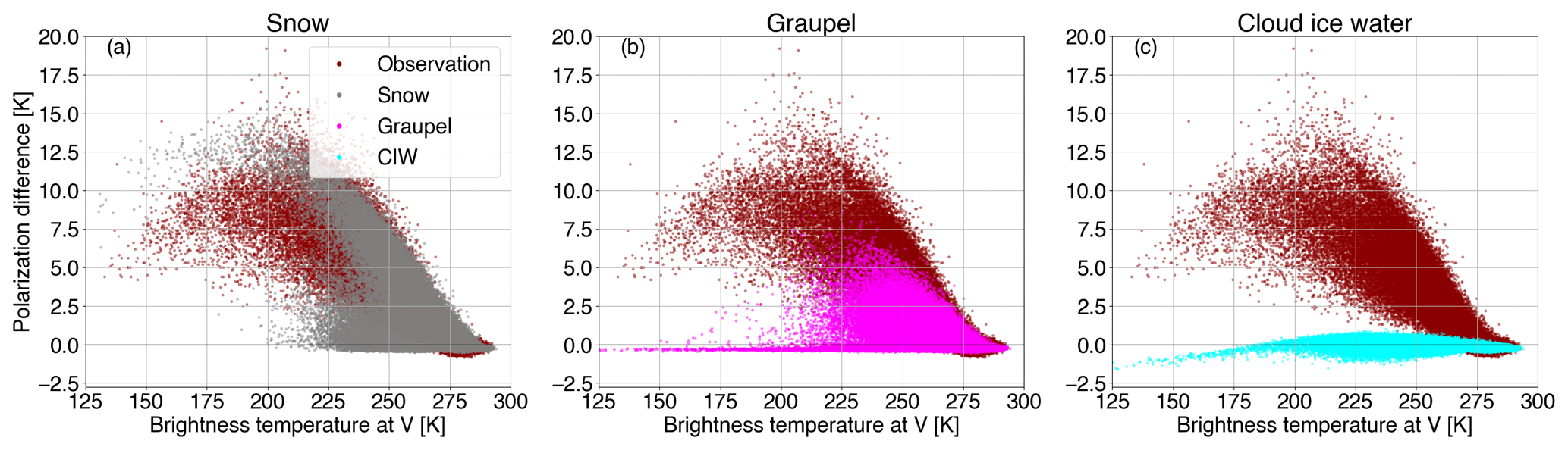
Figure 6As in Fig. 2 but for (a) snow (gray), (b) graupel (magenta), and (c) cloud ice water (CIW; cyan) individually polarized passive monitoring experiments at a polarization ratio of 1.4.
To quantify the contribution of each ice hydrometeor to the total polarization difference (globally), the consistency in the distributions between observations and simulations has been investigated; Fig. 7 illustrates the corresponding histograms and their 1D divergence. Comparing Fig. 5b with Fig. 7a, it follows that snow slightly underestimates PDs between 2 and 11 K, leading to small negative penalty values of φ1D; the overall divergence Φ1D is found to be a bit larger (0.279) than the one resulting from applying the ρ to all of the hydrometeors (0.260). Graupel poorly represents the polarization differences above ≈2.5 K, whereas it completely fails to generate any values above ≈8.5 K; the underestimation increases with increasing PD up to ≈8.5 K and, at larger PD values, any φ1D value is solely linked to the artificial penalty effect, i.e., empty bins are replaced by a population of 0.1, resulting in a total Φ1D value of 1.627. Cloud ice generates a polarization signal between −0.5 and 1.2 K, leading to a much larger total Φ1D (2.859); this is close to the one obtained for the control run, i.e., 3.047.
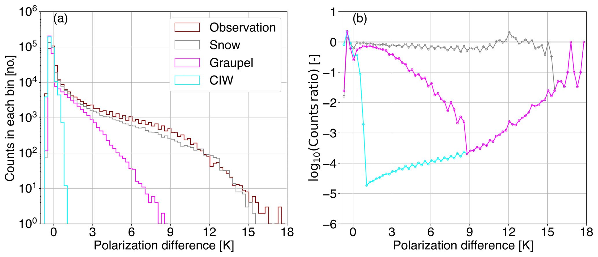
Figure 7Histograms of the polarization differences at 166.5 GHz as observed by GMI (PDo; red) and simulated (PDb) for a polarization ratio of 1.4 applied to (a) snow only (gray), (b) graupel only (magenta), and (c) cloud ice water only (CIW; cyan).
3.4 Forecast impact
As described in Sect. 2.6, cycled DA experiments were run to see whether using polarized scattering in the observation operator for SSMIS, GMI, and AMSR-2 could improve the quality of the forecast. The polarization ratio ρ=1.4 found at 166.5 GHz was used for all ice hydrometeors at all frequencies, but it was applied in three different ways: either with equal and opposite perturbations to V and H channels, as in Eq. (6) where α=0.167, or by unilaterally changing the ice hydrometeor optical depth in only the H or only the V channels:
These latter experiments are equivalent to increasing τH by 40 % (β=0.4) or reducing τV by 29 % (γ=0.286). This is an approximate way to explore whether the polarized scattering might provide better results in combination with an adjustment to the original ice hydrometeor optical depths, which are not themselves known with high accuracy.
First, we evaluate the performance of the polarized correction against independent references by using the observations and channels selected for active DA but not yet assimilated under all-sky conditions (i.e., the observation operator is unchanged); it is essential to ensure that improving polarized scattering for conical scanners does not degrade the data assimilation under clear-sky conditions. For example, Fig. 8 examines the change in quality of the 12 h forecast as measured by the σ of ATMS background departures. The standard deviation, σ, is an appropriate metric of forecast skill here because the distribution of simulated ATMS observations under clear-sky conditions is not expected to change. Starting with the results where ρ=1.4 was applied with equal and opposite perturbations to V and H channels for all three conical scanners, it can be seen that the ATMS tropospheric humidity channels (18–22; around 183.31 GHz) and stratospheric channels (11–15; ≈56.9–57.6 GHz) are not significantly affected. However the tropospheric temperature sounding channels (6–10; ≈53.6–57.3 GHz) show a slight but statistically significant increase in σ, suggesting a minor degradation in forecast quality. To counterbalance this, other conventional data (not shown) showed marginal but significant improvements in forecast quality, suggesting overall a neutral impact.
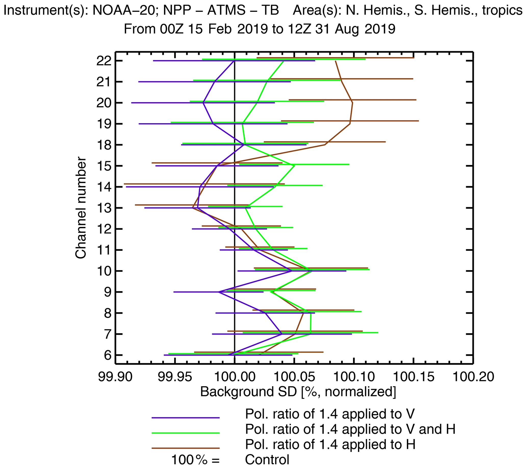
Figure 8Normalized change in the standard deviation (σ) of background (12 h forecast) fits to independent ATMS observations with a polarization ratio (ρ) of 1.4, applied in different ways to the V and H channels. Error bars give the 95 % confidence interval estimated using a paired-difference t test from per-cycle (every 12 h) statistics, without corrections for multiple comparisons.
Slightly different results were seen with the unilateral scaling of the layer optical thickness between the V and H channels. The unilateral increase in H channels appears to give a significant degradation in forecast skill in tropospheric temperature channels (6–10; ≈53.6–57.3 GHz) and humidity channels (18–22; around 183.31 GHz) of ATMS. In contrast, a unilateral decrease in V channels appears to leave forecast skill unchanged. As the overall level of the hydrometeor optical depth decreases (going from H only, to V and H, to V only), it appears that the forecast skill slightly improves. This suggests that it is also important to get the overall level of scattering correct in order to be able to implement the polarized scattering.
Figure 9 shows the normalized change in σ of background departures for two of the sensors for which the polarized scattering correction has been applied (i.e., GMI and SSMIS). Here, changes can come from two sources: a change in the quality of the background forecasts (as for ATMS) or directly due to the change in the observation operator (a least, in channels where the scaling was applied). Regarding this second effect, when the observation operator is modified, the statistics can be affected by the change in the distributions of simulated brightness temperatures; hence, they are vulnerable to the double-penalty effect. For example, adding 40 % to ice hydrometeor optical depths in an H channel like SSMIS 9 (183.31 ± 6.6 GHz; brown line in Fig. 9b) likely explains the 6 % larger σ of background departure. Similarly, reducing extinction by 29 % in V channels such as SSMIS 17 (91.655 GHz; purple line in Fig. 9b) likely explains the reduction in σ by 2 %. Where polarization is applied with equal and opposite perturbations to the V and H channels (green lines) the change in σ appears to be dominated by the double-penalty effect. However, the figure still provides an important result with respect to the benefits of polarized scattering. As shown in Table 2, most of the high-frequency channels of GMI are V polarized (≥89.0 GHz; channels 8, 10, 12, and 13) and most of those on SSMIS are H polarized (≥150.0 GHz; channels 8, 9, 10, and 11). When only the H-channel simulations are modified, the V channels provide an independent measure of the forecast quality. Likewise when only V-channel simulations are modified, the H channels are an independent reference. Adding extinction in H channels (brown lines), i.e., GMI channel 11 (166.5 GHz) and SSMIS channels 8–11 (≈150–183.31 GHz), reduces σ by around 0.5 % in GMI V channels, i.e., channel 10 (166.5 GHz) and 12–13 (≈183.31 GHz), and in SSMIS V-channel 17 (91.655 GHz). Similarly, reducing extinction in V channels (purple lines) reduces σ in SSMIS H channels and in GMI H-channel 11 (166.5 GHz), similarly by around 0.5 %. Results from AMSR-2 (not shown) are equivalent. This suggests that representing polarized scattering makes the forward modeling more consistent across sensors, as well as between channels. At high frequencies (such as the 183.0 GHz channels) SSMIS will generally see bigger scattering depressions than GMI due to the different polarizations; if this effect is not represented in the observation operator, it degrades the consistency of the DA.

At millimeter and submillimeter wavelengths, the interaction between ice hydrometeors and radiation is chiefly driven by scattering (high single scattering albedo; see, e.g., Eriksson et al., 2011). Consequently, such interaction induces a considerable polarization signature that strongly depends on the size, shape, and orientation of the hydrometeors. In other words, nonspherical ice hydrometeors are characterized by non-unit aspect ratios, i.e., the ratio of the longest to the shortest axis, and, if they are large enough, they tend to be oriented in the atmosphere under relatively low turbulence conditions (e.g., stratiform regime or anvil regions of convections). This results in viewing-dependent scattering properties, leading to brightness temperature differences between V- and H-polarized channels, i.e., the polarization difference.
4.1 Polarization differences due to oriented ice hydrometeors
In the GMI observations examined here, the high-frequency dual-polarization channels (89.0 and, particularly, 166.5 GHz) show a global arch-like relationship between PD and TBV, confirming the findings of Gong and Wu (2017) and Brath et al. (2020) over the same frequencies and Defer et al. (2014) at the slightly lower frequency of MADRAS (i.e., 157.0 GHz). The arch-like relationship is generally attributed to two processes: the saturation of polarization under conditions of multiple scattering and the composition of the hydrometeors (size, shape, and orientation) within a dynamic environment. Increasing the number of sufficiently large (≈ 40–150 µm depending on shape) horizontally oriented nonspherical ice hydrometeors (e.g., flat plates, columns, and fluffy snow aggregates) under relatively low turbulence conditions (e.g., stratiform regime or anvil regions of convections) leads to an increasing scattering and, hence, a stronger polarization signal (e.g., Spencer et al., 1989; Gong and Wu, 2017; Gong et al., 2020; Brath et al., 2020). However, the final polarization state results from only the first few orders of scattering (similar effects are seen at visible frequencies; see, e.g., Barlakas (2016) and references therein). Hence, an increasing multiple-scattering process due to the presence of enough hydrometeors will initially lead to a saturation (plateau) of the polarization and then to a further decrease in the PD. Accordingly, the low PD values are found at warm TBV (≈275 K), corresponding to very thin clouds, whereas the largest values are linked to intermediate cold TBV and medium thick clouds, particularly in the anvil regions of convection. Within deep convective cores (at increasingly low TBV), tumbling motions may lead to the formation of less oblate hydrometeors (i.e., hail and graupel; Jung et al., 2008), disrupt any hydrometeor orientation inducing either higher tilt angles (see Fig. 1) or even total random orientation, and together with the enhanced multiple-scattering process, lead to low or absent PD (≈0–7 K) (e.g., Spencer et al., 1989; Gong and Wu, 2017; Gong et al., 2020).
In contrast to 89.0 GHz (see Fig. A1a), the arch-like shape of PD–TBV at 166.5 GHz (see Fig. 4a) is characterized by a greater dynamical range (≈140–275 K compared with ≈170–275 K), in line with the results reported by Gong and Wu (2017), Galligani et al. (2021), and Defer et al. (2014), and peaks at larger PD values (≈14 K compared with ≈10 K). The lower PD found at 89.0 GHz could be explained by its multi-sensitivity aspect: a frequency of 89.0 GHz is quite sensitive to water vapor, water cloud, and rain droplets that could diminish the polarization signal due to emission, especially if there is a liquid layer below the ice hydrometeor layer.
4.2 Approximate treatment of polarized scattering from oriented ice hydrometeors
In the current framework of RTTOV-SCATT, only TRO hydrometeors are considered, which fails to reproduce the observed PDs, leading to errors in polarized scattering up to about 10–15 K. To model the effect of preferentially oriented (ARO) ice hydrometeors, a simple correction scheme has been implemented in RTTOV-SCATT that reduces TRO extinction in V-polarized channels and increases it in H-polarized ones. This is quantified by the ratio of extinction in H channels over that in V channels, i.e., the polarization ratio ρ. This ratio holds an indirect microphysical representation of the aspect ratio of nonspherical oriented hydrometeors.
Totally randomly oriented hydrometeors (control run) are characterized by a ρ of 1.0 and cannot induce polarization in our modeling framework. For the dual-polarization channels, the values of ρ that best approximate the orientation of nonspherical ice hydrometeors and yield a more symmetrical error are 1.5 and 1.4 for 89.0 and 166.5 GHz, respectively. For example, the mean error in the differences in PD between simulations and observations (PDo−PDb) is diminished by an order of magnitude at 166.5 GHz. These values of ρ are equivalent to adjusting the extinction of the control run by ±20 % (α=0.20) at 89.0 GHz and by ±16.7 % (α=0.167) at 166.5 GHz in order to match the extinction at the two polarization components. In addition, at 166.5 GHz, it approximates the magnitude of the K12 element of the extinction matrix quite well in the case of ARO (KARO,12) at a tilt angle of 0∘ (see Fig. 1b; in the case of large plate aggregates), which describes the actual differences in the extinction between the H and V polarization. Recall here that α in Eq. (6) approximates the magnitude of KARO,12 at Earth incident angles of around 55∘. These findings are in line with those reported by Brath et al. (2020). The values of ρ are valid at a global scale (over both land and ocean), with a higher confidence at 166.5 GHz.
Figure 4b shows that, for a ρ value of 1.4, the polarized correction scheme in RTTOV-SCATT is able to do a reasonable job of reproducing the observed scattering arches; however, compared with observations it tends to over-favor larger PDs at the peak of the arch (e.g., at 200 K) or low PD values (0–2 K) at the lower part of the arch (e.g., K), whereas PDs do not drop low enough at lower TBV (e.g., 150 K). RTTOV-SCATT does not simulate the full arch-like relationship because it cannot transfer energy from one polarization to the other (the multiple-scattering effect). In addition, Geer (2021) reported that the combination of the IFS and RTTOV-SCATT does not simulate deep enough brightness temperature depressions in tropical convection over land (see also Fig. 5a), likely due to insufficient horizontal spreading of the upper glaciated parts of the convective cloud; these scenes, if represented correctly, should have lower PDs according to the hypothesis that turbulence in the deep convective core is responsible for random orientation and, hence, depolarization. However, it does reproduce some of the drop in polarization in strongly scattering scenes which is likely due to saturation of the scattering; the differences between τH and τV become irrelevant. Ideally, the choice of ρ would be situation dependent. However, this would increase the intricacy of the forward operator and further complicates any attempts to impartially certify the impact of such a correction scheme.
Going back to the optimum choice of the ρ, at 89.0 GHz, a more symmetrical error is achieved at a ratio of 1.45 over the ocean (1.5 overall), although this could be attributed to the relatively low number of pixels fulfilling the rather strict screening method which minimizes the strongly polarizing ocean surface. The IFS simulates (with slightly low confidence) this channel quite differently over land and the ocean. This is partially due to its aforementioned multi-sensitivity aspect that complicates radiative transfer. Accordingly, some polarization signal simulated at this frequency could originate from strongly polarizing inland water (e.g., large lakes or flooding) that have not been perfectly screened or even from shallow clouds over ocean at high latitudes. Similar patterns of potential surface contamination have been recently reported by Galligani et al. (2021). Furthermore, liquid droplets can be horizontally aligned, inducing small PDs (≈0.5 K, Ekelund et al., 2020) that are observed but not simulated in the IFS. All of these factors, in addition to the known limitations of the IFS and RTTOV-SCATT in representing convective systems (Geer, 2021), could potentially explain the rather large polarization ratio required to obtain reasonable simulations (good fit to the observations) at 89.0 GHz.
Given that larger PDs are found at 166.5 GHz than at 89.0 GHz, it might seem obvious that there should also be a larger polarization ratio at 166.5 GHz. However, this makes the incorrect assumptions that the level of extinction is the same for both frequencies and that the frequencies are sensitive to the same size range of hydrometeors. In fact, the PD has a complex dependence on parameters such as size, shape, aspect ratio, PSD, and the channel’s frequency and the level of extinction (Xie and Miao, 2011; Defer et al., 2014). Lower frequencies are more sensitive to larger hydrometeors (e.g., Buehler et al., 2007), and it is likely that the axial ratio and, thus, the orientation increase with size. This effect would suggest a larger PD at 89.0 GHz. Further, the extinction generated by ice hydrometeors is smaller at 89.0 GHz; thus, if all else were constant, obtaining the same PD at 89.0 GHz as at 166.5 GHz would also require a higher polarization ratio at 89.0 GHz. Putting aside the small differences between the best polarization ratio at each frequency, the values found in this study are reasonably consistent with other studies, such as the ratios of 1.2–1.4 reported by Gong and Wu (2017) for the same dual-polarization channels of GMI. In the studies of Davis et al. (2005) and Defer et al. (2014), it is not the polarization ratio but the actual microphysical aspect ratio that is reported, so it is hard to make an exact comparison. However, Davis et al. (2005) found similar aspect ratios at the lower-frequency channel of 122.0 GHz of the Earth Observing System (EOS) Microwave Limb Sounder (MLS). On the other hand, Defer et al. (2014) suggested an aspect ratio of 1.6 to be the most realistic one for reproducing the PDs observed by MADRAS at both 89.0 and 157.0 GHz. In any case, these ratios are all subject to the microphysical representation of the hydrometeors employed, so a hydrometeor type with a different scattering efficiency would result in a different ratio.
4.3 Linking the polarization difference to a hydrometeor type
The polarization signal prompted by preferentially oriented hydrometeors strongly depends on their microphysical representation. To further interpret this signal, ρ was applied to each ice hydrometeor individually. Horizontally oriented large-scale snow and deep convective snow (graupel) are responsible for causing most of the observed PDs at 166.5 GHz, which is consistent with Brath et al. (2020), with snow being associated with the largest PD values as also addressed by Defer et al. (2014) and Gong and Wu (2017). Comparing the snow- and graupel-only scaled simulations, the former produces PD values across the entire range, whereas the latter is responsible for generating mostly low to medium PDs at warm to intermediate cold TBV (270 to 210 K). This is thought to come from the representation of convection in the forecast model and RTTOV-SCATT, as it occupies only 5 % of the model grid box. Even if a convective column generates strongly polarized scattering in RTTOV-SCATT, this limits its effect on the whole-scene brightness temperatures. In contrast, precipitation generated by the large-scale scheme typically occupies a large fraction of the grid box and is able to generate stronger PDs in the complete scene.
In reality, similar behaviors are observed, but they are driven by different processes (Gong and Wu, 2017; Gong et al., 2020). In the case of snow, the tumbling motions in the ambient environment and the two-fold scattering effect described in Sect. 4.1 can explain the observed polarization patterns. A plausible interpretation of the different polarization signal induced by graupel is its higher weight and the tumbling motions within deep convective cores that lead to less oblate shapes (Jung et al., 2008): for the same amount of hydrometeors, it will be less oriented, resulting in lower PD values.
Although one could assume that cloud ice hydrometeors are too small to induce any polarization at 166.5 GHz, the cloud-ice-only scaled simulations conducted here suggest a minor PD (less than 1.2 K) with a preference for negative values at low brightness temperatures. Representing the cloud ice by the large column aggregate habit and the PSD introduced by Heymsfield et al. (2013) can potentially lead to large enough hydrometeors and, hence, to enough scattering to induce a visible polarization signal. This supports the suggestion by Gong et al. (2020) that some smaller PDs at 166.5 GHz may come from cloud ice. At warmer temperatures, negative PDs at 166.5 GHz were reported by Gong and Wu (2017); they linked this to clear-sky conditions and instrumental noise. At colder temperatures, they also saw negative PDs, without providing any clear explanation. Here, negative PD values are simulated in deep convective areas (TBV below 180 K). The most likely explanation is that RTTOV-SCATT is representing cloud ice above deep convection with relatively low single-scattering albedos; hence, there is an emission signal that is stronger in the H channels due to the stronger extinction. In reality, negative PDs are also measured (Davis et al., 2005; Prigent et al., 2005), with the most dominant interpretation being the vertical orientation of hydrometeors. A likely explanation of the vertical orientation is lightning activities at cloud top (hydrometeor electrification) of deep convective systems (Prigent et al., 2005). However, RTTOV-SCATT does not represent vertically oriented hydrometeors; therefore, if it is able to simulate a negative PD through absorption, it suggests that the electrification hypothesis may only be one part of the story.
Herein, an effort has been carried out to improve the physical representation of polarized scattering in RTTOV-SCATT (Radiative Transfer model for TOVS that accounts for multiple scattering) and to explore whether such an improvement would have an impact on the forecast of the European Centre for Medium-Range Weather Forecasts (ECMWF). To approximate the effect of oriented ice hydrometeors in reproducing the observed brightness temperature (TB) differences between vertical (V) and horizontal (H) polarization, i.e., the polarization difference (), from conical scanning sounders, the layer optical thickness of these hydrometeors is increased in the H and decreased in the V channels. This is governed by the assumed polarization ratio (ρ).
By optimizing measures of fit between dual-polarization observations from the Global Precipitation Mission (GPM) microwave imager (GMI) and simulations from the Integrated Forecast System (IFS) of ECMWF, it follows that the value of ρ that best models the orientation of ice hydrometeors is 1.5 at 89.0 GHz and 1.4 at 166.5 GHz, with lower confidence at 89.0 GHz. With these settings, RTTOV-SCATT is capable of simulating the effect of oriented hydrometeors, and it generates a reasonable representation of the observed arch-like relationship between PD and TBV (or TBH). This reduces the maximum modeling errors in PD by about 10–15 K. Although the simulated PD is not perfect, the discrepancies in PD between observations and simulations are ameliorated, by an order of magnitude at 166.5 GHz, and the remaining errors are now approximately symmetrical. In the context of data assimilation (DA), assigned observation errors are quite large (e.g., up to 35 K in terms of the PD for the GMI 166.5 GHz channels in deep convective areas), but a 15 K error reduction would still be a significant improvement.
Applying ρ to each ice hydrometeor type individually, we demonstrated that the polarization signal strongly depends on their microphysical representation. Assuming that IFS gives a fair representation of the real atmosphere, it is suggested that snow and graupel are responsible for causing most of the observed polarization signal, with snow producing PD values across the entire range and graupel generating mostly low to medium PDs at warm to intermediate cold brightness temperatures. Where only cloud ice was polarized, simulations give a negative polarization signal over deep convection or heavy precipitation, which could potentially be linked to enhanced emission effects in the H channels.
Cycling DA experiments were used to examine the impact of representing polarized scattering in the observation operators for the conical scanners: GMI, Special Sensor Microwave Imager/Sounder (SSMIS), and Advanced Microwave Scanning Radiometer-2 (AMSR-2). This was conducted for a polarization ratio of 1.4 applied to all ice species and all channels. Validation against independent references (i.e., instruments employed in DA but where the observation operator was unchanged; clear-sky DA) showed mixed but broadly neutral changes to forecast quality – in other words, the improved modeling of the polarization difference does not appear to affect the broader forecast quality. However, some semi-independent validation was possible using the conical scanners to which the polarization correction was applied: this showed that when the desired ρ was achieved with a unilateral scaling (e.g., in V channels), it was possible to see positive impacts in the forecast skill measured by the conical sounder channels in H channels, and vice versa. This suggests that representing polarization makes the forward operator more consistent between V and H channels of the same instrument as well as between instruments with different polarizations. For example, at high frequencies (e.g., ≈183.0 GHz), SSMIS will generally see bigger scattering depressions than GMI due to the different polarizations. Thus, if SSMIS and GMI both observe the same feature (even at different times during the assimilation window or in different windows), the representation of polarized scattering would allow the DA scheme to make more consistent corrections to the forecast. This likely improves the consistency of the forecast in areas of cloud and precipitation (e.g., frontal areas).
A second implication from the cycling DA experiments came from noting that a unilateral decrease in scattering in V channels gave marginally better results (versus independent humidity-sensitive observations), whereas the unilateral increase in H channels gave marginally worse results. This suggests the need to tune the overall level of scattering in RTTOV-SCATT. This is particularly necessary as the selection of hydrometeor assumptions used for this work was tuned against instruments with predominantly H-polarization channels at high frequencies (e.g., Geer, 2021, used SSMIS). Hence, Geer (2021) carried out a further retuning of the microphysical assumptions, considering the polarization scheme introduced here, with a default ρ value of 1.4 for all ice species at all channels. That final retuning, along with the new polarization scheme, provides the final configuration for RTTOV-SCATT version 13 (v13.0). This configuration is also aimed at implementation in a future cycle of the IFS.
The performance of this polarization scheme has only been tested with conical scanning sounders, and it is likely valid only at Earth incident angles around 55∘, where hydrometeor orientation does not change the overall level of extinction (the K11 term in the Brath et al., 2020, database, as presented in Sect. 2.5). Modeling the effect of hydrometeor orientation at other angles will require significant further work, as both the overall extinction and the degree of polarization must vary as a function of the Earth incident angle. For cross-track microwave sounders this will be particularly difficult, as they are not currently equipped with high-frequency dual-polarization channels with which to validate the results and the polarization rotates across the swath. Future work could also aim at developing a similar correction scheme for radar backscattering. A subsequent step would be to explore the performance of ρ at higher submillimeter wavelengths; the upcoming Ice Cloud Imager (ICI) mission, with dual-polarization channels at frequencies that are sensitive to the column scattering due to ice hydrometeors (243.2 and 664.4 GHz), will provide further insights regarding the polarization signal due to small oriented ice hydrometeors.
To minimize the surface contribution, the clear-sky surface-to-space transmittance (t) simulated by RTTOV has been employed. Recall here that the superscript b corresponds to the simulated (background) quantities. Accordingly, the surface contribution to the polarization can be approximated (ignoring the downward radiance term) by
where eV and eH are the surface emissivities at V and H polarization, respectively, Tsfc is the surface temperature, and t166.5 denotes the transmittance at 166.5 GHz. An upper threshold t166.5 value of 0.05 has been adopted to mask out the surface contribution at both dual-polarization channels. This can be translated (via Eq. A1) to a maximum surface-induced polarization difference of 2.9 K. Lower values of the clear-sky t166.5 have been also tested, i.e., 0.01–0.04 (0.58–2.32 K in PD), to ensure that the polarization signature originates from oriented ice hydrometeors and not from clear-sky conditions and, thus, from the surface. To isolate cloudy GMI pixels, we additionally defined the hydrometeor impact as follows:
Here, () represents the hydrometeor impact defined by the observed (simulated) brightness temperature under all-sky conditions minus the simulated equivalent atmosphere without clouds. Any situation with a hydrometeor impact above 0 K is rejected; this is done on a channel-wise basis, and the rejection is done if either observations or simulations cross this threshold. The bias correction is included at 166.5 GHz, but it is excluded at 89.0 GHz because it led to a mismatch between observations and simulations. This two-fold screening method does not completely eliminate surface polarization signatures at 89.0 GHz. Hence, an additional basic filtering has been applied to this channel only. First, pixels where the control run yields a PDb greater than 1 K are masked out, as the control run does not produce any polarization due to preferentially oriented hydrometeors. Second, pixels where the observed PD (PDo) is greater than 5 K and K are excluded (this is the visible rectangular bite out of the distribution in Fig. B1a).
Figure A1a displays the performance of the screening method at a scene measured by GMI on 13 July 2019 at 166.5 GHz. This method minimizes any surface contamination, although it is rather strict and screens out thin cirrus clouds, especially over the midlatitudes. Figure A1b demonstrates the rather good performance of the polarization ratio (ρ) of 1.4 to simulate PDo.

Figure A1Performance of the screening method at an example scene measured by GMI on 13 July 2019 at a frequency of 166.5 GHz. Polarization difference, i.e., brightness temperature differences between the vertical and horizontal polarization (), due to oriented ice hydrometeors as (a) observed (PDo) by GMI and (b) simulated (PDb) for a polarization ratio (ρ) of 1.4.
Figure B1 displays the two-dimensional (2D) histogram of the arch-like relationship between the polarization difference and the brightness temperature at V polarization at 89.0 GHz as observed by GMI (Fig. B1a), simulated for a ρ of 1.5 (Fig. B1b), and the corresponding 2D histogram divergence (Fig. B1c). Simulations fail to reproduce the full arch-like shape. Due to the screening method, most moderately cloudy scenes over the ocean have been excluded, leading to a rather small sample; however, the main PDo branch ( K) and the PDo peak (≈10 K) have been modeled quite well by a ρ value of 1.5.
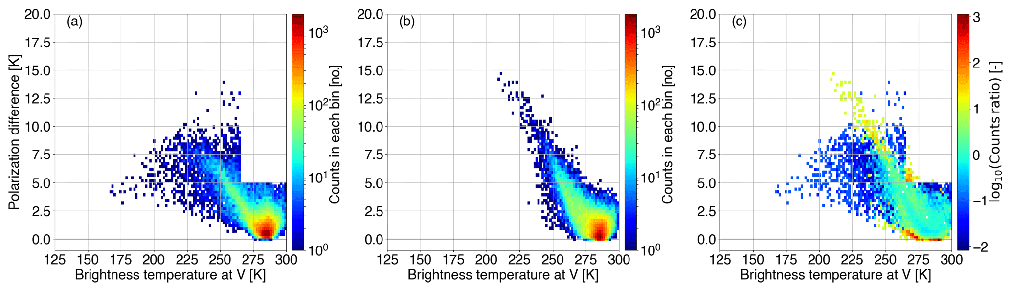
Figure B1Two-dimensional (2D) histograms describing the arch-like relationship between the polarization difference and the brightness temperature at V polarization at 89.0 GHz as (a) observed (PDo–) by GMI, (b) simulated (PDb–) for a polarization ratio of 1.5, and (c) the 2D histogram divergence between (PDo–) and (PDb–). In panel (c), white areas denote the case where both the observed and the simulated 2D bins are empty.
The RTTOV-SCATT model can be obtained at https://nwp-saf.eumetsat.int/site/software/rttov/ (Saunders et al., 2018) – registration is required. Due to the large volume of data generated by the IFS assimilation experiments, permanent archiving and curation is not possible. However, reanalysis data, such as ERA-5 (the fifth generation of the ECMWF atmospheric reanalyses of the global climate), are available at https://cds.climate.copernicus.eu/#!/home (Hersbach et al., 2020).
The work was conceptualized and refined by VB, AJG, and PE. Writing, coding, and analysis were mainly carried out by VB, with contributions from AJG.
The authors declare that they have no conflict of interest.
The work of Vasileios Barlakas at Chalmers University of Technology is funded by a EUMETSAT fellowship program. Niels Bormann, Luisa Ickes, Franz Kanngiesser, Inderpreet Kaur, and Simon Pfreundschuh are thanked for the many thoughtful comments that led to the overall improvement of the paper.
This research has been supported by a EUMETSAT fellowship program.
This paper was edited by S. Joseph Munchak and reviewed by three anonymous referees.
Aires, F., Prigent, C., Bernardo, F., Jiménez, C., Saunders, R., and Brunel, P.: A Tool to Estimate Land-Surface Emissivities at Microwave frequencies (TELSEM) for use in numerical weather prediction, Q. J. Roy. Meteorol. Soc., 137, 690–699, https://doi.org/10.1002/qj.803, 2011. a
Auligné, T., McNally, A. P., and Dee, D. P.: Adaptive bias correction for satellite data in a numerical weather prediction system, Q. J. Roy. Meteorol. Soc., 133, 631–642, https://doi.org/10.1002/qj.56, 2007. a
Baordo, F. and Geer, A. J.: Assimilation of SSMIS humidity-sounding channels in all-sky conditions over land using a dynamic emissivity retrieval, Q. J. Roy. Meteorol. Soc., 142, 2854–2866, https://doi.org/10.1002/qj.2873, 2016. a
Barlakas, V.: A new three-dimensional vector radiative transfer model and applications to Saharan dust fields, PhD thesis, University of Leipzig, Leipzig, Germany, available at: https://nbn-resolving.org/urn:nbn:de:bsz:15-qucosa-207467 (last access: 4 November 2020), 2016. a, b, c
Barlakas, V. and Eriksson, P.: Three dimensional radiative effects in passive millimeter/sub-millimeter all-sky observations, Remote Sens., 12, 531, https://doi.org/10.3390/rs12030531, 2020. a
Bauer, P., Moreau, E., Chevallier, F., and O'keeffe, U.: Multiple-scattering microwave radiative transfer for data assimilation applications, Q. J. Roy. Meteorol. Soc., 132, 1259–1281, https://doi.org/10.1256/qj.05.153, 2006. a
Brath, M., Ekelund, R., Eriksson, P., Lemke, O., and Buehler, S. A.: Microwave and submillimeter wave scattering of oriented ice particles, Atmos. Meas. Tech., 13, 2309–2333, https://doi.org/10.5194/amt-13-2309-2020, 2020. a, b, c, d, e, f, g, h, i, j, k, l, m
Buehler, S. A., Jiménez, C., Evans, K. F., Eriksson, P., Rydberg, B., Heymsfield, A. J., Stubenrauch, C. J., Lohmann, U., Emde, C., John, V. O., Sreerekha, T. R., and Davis, C. P.: A concept for a satellite mission to measure cloud ice water path, ice particle size, and cloud altitude, Q. J. Roy. Meteorol. Soc., 133, 109–128, https://doi.org/10.1002/qj.143, 2007. a
Czekala, H.: Effects of ice particle shape and orientation on polarized microwave radiation for off-nadir problems, Geophys. Res. Lett., 25, 1669–1672, https://doi.org/10.1029/98GL51132, 1998. a, b, c
Davis, C. P., Wu, D. L., Emde, C., Jiang, J. H., Cofield, R. E., and Harwood, R. S.: Cirrus induced polarization in 122 GHz aura Microwave Limb Sounder radiances, Geophys. Res. Lett., 32, L14806, https://doi.org/10.1029/2005GL022681, 2005. a, b, c, d, e, f
Dee, D.: Variational bias correction of radiance data in the ECMWF system, ECMWF Workshop on Assimilation of high spectral resolution sounders in NWP, Shinfield Park, Reading, UK, 28 June–1 July 2004, available at: https://www.ecmwf.int/node/8930 (last access: 4 May 2021), 97–112, 2004. a
Defer, E., Galligani, V. S., Prigent, C., and Jiménez, C.: First observations of polarized scattering over ice clouds at close-to-millimeter wavelengths (157 GHz) with MADRAS on board the Megha-Tropiques mission, J. Geophys. Res.-Atmos., 119, 12301–12316, https://doi.org/10.1002/2014JD022353, 2014. a, b, c, d, e, f, g, h, i, j
Du, J., Kimball, J. S., Jones, L. A., Kim, Y., Glassy, J., and Watts, J. D.: A global satellite environmental data record derived from AMSR-E and AMSR2 microwave Earth observations, Earth Syst. Sci. Data, 9, 791–808, https://doi.org/10.5194/essd-9-791-2017, 2017. a
Duncan, D. I. and Eriksson, P.: An update on global atmospheric ice estimates from satellite observations and reanalyses, Atmos. Chem. Phys., 18, 11205–11219, https://doi.org/10.5194/acp-18-11205-2018, 2018. a
Ekelund, R., Eriksson, P., and Pfreundschuh, S.: Using passive and active observations at microwave and sub-millimetre wavelengths to constrain ice particle models, Atmos. Meas. Tech., 13, 501–520, https://doi.org/10.5194/amt-13-501-2020, 2020. a
Eriksson, P., Rydberg, B., and Buehler, S. A.: On cloud ice induced absorption and polarisation effects in microwave limb sounding, Atmos. Meas. Tech., 4, 1305–1318, https://doi.org/10.5194/amt-4-1305-2011, 2011. a
Eriksson, P., Jamali, M., Mendrok, J., and Buehler, S. A.: On the microwave optical properties of randomly oriented ice hydrometeors, Atmos. Meas. Tech., 8, 1913–1933, https://doi.org/10.5194/amt-8-1913-2015, 2015. a
Eriksson, P., Ekelund, R., Mendrok, J., Brath, M., Lemke, O., and Buehler, S. A.: A general database of hydrometeor single scattering properties at microwave and sub-millimetre wavelengths, Earth Syst. Sci. Data, 10, 1301–1326, https://doi.org/10.5194/essd-10-1301-2018, 2018. a, b, c, d, e
Eriksson, P., Rydberg, B., Mattioli, V., Thoss, A., Accadia, C., Klein, U., and Buehler, S. A.: Towards an operational Ice Cloud Imager (ICI) retrieval product, Atmos. Meas. Tech., 13, 53–71, https://doi.org/10.5194/amt-13-53-2020, 2020. a
Evans, K. F. and Stephens, G. L.: Microwave radiative transfer through clouds composed of realistically shaped ice crystals. Part I. Single scattering properties, J. Atmos. Sci., 52, 2041–2057, https://doi.org/10.1175/1520-0469(1995)052<2041:MRTTCC>2.0.CO;2, 1995a. a
Evans, K. F. and Stephens, G. L.: Microweve radiative transfer through clouds composed of realistically shaped ice crystals. Part II. Remote sensing of ice clouds, J. Atmos. Sci., 52, 2058–2072, https://doi.org/10.1175/1520-0469(1995)052<2058:MRTTCC>2.0.CO;2, 1995b. a
Field, P. R., Heymsfield, A. J., and Bansemer, A.: Snow size distribution parameterization for midlatitude and tropical ice clouds, J. Atmos. Sci., 64, 4346–4365, https://doi.org/10.1175/2007JAS2344.1, 2007. a, b, c, d, e
Forbes, R., Tompkins, A., and Untch, A.: A new prognostic bulk microphysics scheme for the IFS, ECMWF, p. 22, https://doi.org/10.21957/bf6vjvxk, 2011. a
Fox, S.: An evaluation of radiative transfer simulations of cloudy scenes from a numerical weather prediction model at sub-millimetre frequencies using airborne observations, Rem. Sens., 12, 2758, https://doi.org/10.3390/rs12172758, 2020. a
Galligani, V. S., Wang, D., Corrales, P. B., and Prigent, C.: A parameterization of the cloud scattering polarization signal derived from GPM observations for microwave fast radiative transfer models, IEEE Trans. Geosci. Remote Sens., 1–10, https://doi.org/10.1109/TGRS.2021.3049921, 2021. a, b, c
Geer, A. J.: Physical characteristics of frozen hydrometeors inferred with parameter estimation, Atmos. Meas. Tech. Discuss. [preprint], https://doi.org/10.5194/amt-2021-50, in review, 2021. a, b, c, d, e, f
Geer, A. J. and Baordo, F.: Improved scattering radiative transfer for frozen hydrometeors at microwave frequencies, Atmos. Meas. Tech., 7, 1839–1860, https://doi.org/10.5194/amt-7-1839-2014, 2014. a, b, c, d, e, f, g, h, i, j
Geer, A. J. and Bauer, P.: Enhanced use of all-sky microwave observations sensitive to water vapour, cloud and precipitation, ECMWF, p. 41, https://doi.org/10.21957/mi79jebka, 2010. a
Geer, A. J., Bauer, P., and O'Dell, C. W.: A revised cloud overlap scheme for fast microwave radiative transfer in rain and cloud, J. Appl. Meteoro. Climatol., 48, 2257–2270, https://doi.org/10.1175/2009JAMC2170.1, 2009a. a
Geer, A. J., Forbes, R., and Bauer, P.: Cloud and precipitation overlap in simplified scattering radiative transfer, available at: https://www.ecmwf.int/node/9516 (last access: 4 November 2020), p. 12, 2009b. a
Geer, A. J., Baordo, F., Bormann, N., Chambon, P., English, S. J., Kazumori, M., Lawrence, H., Lean, P., Lonitz, K., and Lupu, C.: The growing impact of satellite observations sensitive to humidity, cloud and precipitation, Q. J. Roy. Meteorol. Soc., 143, 3189–3206, https://doi.org/10.1002/qj.3172, 2017. a, b
Geer, A. J., Lonitz, K., Weston, P., Kazumori, M., Okamoto, K., Zhu, Y., Liu, E. H., Collard, A., Bell, W., Migliorini, S., Chambon, P., Fourrié, N., Kim, M.-J., Köpken-Watts, C., and Schraff, C.: All-sky satellite data assimilation at operational weather forecasting centres, Q. J. Roy. Meteorol. Soc., 144, 1191–1217, https://doi.org/10.1002/qj.3202, 2018. a, b
Gong, J. and Wu, D. L.: Microphysical properties of frozen particles inferred from Global Precipitation Measurement (GPM) Microwave Imager (GMI) polarimetric measurements, Atmos. Chem. Phys., 17, 2741–2757, https://doi.org/10.5194/acp-17-2741-2017, 2017. a, b, c, d, e, f, g, h, i, j, k, l, m, n, o
Gong, J., Zeng, X., Wu, D. L., Munchak, S. J., Li, X., Kneifel, S., Ori, D., Liao, L., and Barahona, D.: Linkage among ice crystal microphysics, mesoscale dynamics, and cloud and precipitation structures revealed by collocated microwave radiometer and multifrequency radar observations, Atmos. Chem. Phys., 20, 12633–12653, https://doi.org/10.5194/acp-20-12633-2020, 2020. a, b, c, d, e
Hersbach, H., Bell, B., Berrisford, P., Hirahara, S., Horányi, A., Muñoz-Sabater, J., Nicolas, J., Peubey, C., Radu, R., Schepers, D., Simmons, A., Soci, C., Abdalla, S., Abellan, X., Balsamo, G., Bechtold, P., Biavati, G., Bidlot, J., Bonavita, M., De Chiara, G., Dahlgren, P., Dee, D., Diamantakis, M., Dragani, R., Flemming, J., Forbes, R., Fuentes, M., Geer, A., Haimberger, L., Healy, S., Hogan, R. J., Hólm, E., Janisková, M., Keeley, S., Laloyaux, P., Lopez, P., Lupu, C., Radnoti, G., de Rosnay, P., Rozum, I., Vamborg, F., Villaume, S., and Thépaut, J.-N.: The ERA5 global reanalysis, Q. J. Roy. Meteorol. Soc., 146, 1999–2049, https://doi.org/10.1002/qj.3803, 2020 (data available at: https://cds.climate.copernicus.eu/#!/home, last access: 4 May 2021). a
Heymsfield, A. J., Schmitt, C., and Bansemer, A.: Ice cloud particle size distributions and pressure-dependent terminal velocities from in situ observations at temperatures from 0∘ to −86 ∘C, J. Atmos. Sci., 70, 4123–4154, https://doi.org/10.1175/JAS-D-12-0124.1, 2013. a, b, c, d
Joseph, J. H., Wiscombe, W. J., and Weinman, J. A.: The delta-Eddington approximation for radiative flux transfer, J. Atmos. Sci., 33, 2452–2459, https://doi.org/10.1175/1520-0469(1976)033<2452:TDEAFR>2.0.CO;2, 1976. a
Jung, Y., Zhang, G., and Xue, M.: Assimilation of simulated polarimetric radar data for a convective storm using the ensemble Kalman filter. Part I: Observation operators for reflectivity and polarimetric variables, Mon. Weather Rev., 136, 2228–2245, https://doi.org/10.1175/2007MWR2083.1, 2008. a, b
Karbou, F., Gérard, E., and Rabier, F.: Global 4DVAR assimilation and forecast experiments using AMSU observations over land. Part I: Impacts of various land surface emissivity parameterizations, Weather Forecast., 25, 5–19, https://doi.org/10.1175/2009WAF2222243.1, 2010. a
Kazumori, M. and English, S. J.: Use of the ocean surface wind direction signal in microwave radiance assimilation, Q. J. Roy. Meteorol. Soc., 141, 1354–1375, https://doi.org/10.1002/qj.2445, 2015. a
Khvorostyanov, V. I. and Curry, J. A.: Thermodynamics, kinetics, and microphysics of clouds, Cambridge University Press, Cambridge UK, https://doi.org/10.1017/CBO9781139060004, 2014. a
Klett, J. D.: Orientation model for particles in turbulence, J. Atmos. Sci., 52, 2276–2285, https://doi.org/10.1175/1520-0469(1995)052<2276:OMFPIT>2.0.CO;2, 1995. a, b, c
Liu, G.: A database of microwave single-scattering properties for nonspherical ice particles, B. Am. Meteorol. Soc., 89, 1563–1570, https://doi.org/10.1175/2008BAMS2486.1, 2008. a, b, c, d
Liu, Q. and Boukabara, S.: Community Radiative Transfer Model (CRTM) applications in supporting the Suomi National Polar-orbiting Partnership (SNPP) mission validation and verification, Remote Sens. Environ., 140, 744–754, https://doi.org/10.1016/j.rse.2013.10.011, 2014. a
Marshall, J. S. and Palmer, W. M. K.: The distribution of raindrops with size, J. Meteorol., 5, 165–166, https://doi.org/10.1175/1520-0469(1948)005<0165:TDORWS>2.0.CO;2, 1948. a
McFarquhar, G. M. and Heymsfield, A. J.: Parameterization of tropical cirrus ice crystal size distributions and implications for radiative transfer: results from CEPEX, J. Atmos. Sci., 54, 2187–2200, https://doi.org/10.1175/1520-0469(1997)054<2187:POTCIC>2.0.CO;2, 1997. a, b
Meissner, T. and Wentz, F.: The emissivity of the ocean surface between 6 and 90 GHz over a large range of wind speeds and earth incidence angles, IEEE T. Geosci. Remote, 50, 3004–3026, https://doi.org/10.1109/TGRS.2011.2179662, 2012. a
Mishchenko, M., Hovenier, J., and Travis, L.: Light scattering by nonspherical particles: theory, measurements, and applications, Elsevier Science, San Diego, California, USA, 1999. a, b, c
Mishchenko, M. I. and Yurkin, M. A.: On the concept of random orientation in far-field electromagnetic scattering by nonspherical particles, Opt. Lett., 42, 494–497, https://doi.org/10.1364/OL.42.000494, 2017. a, b
Noel, V. and Sassen, K.: Study of planar ice crystal orientations in ice clouds from scanning polarization lidar observations, J. Appl. Meteorol., 44, 653–664, https://doi.org/10.1175/JAM2223.1, 2005. a
Petty, G. W. and Huang, W.: The modified gamma size distribution applied to inhomogeneous and nonspherical Particles: Key Relationships and Conversions, J. Atmos. Sci., 68, 1460–1473, https://doi.org/10.1175/2011JAS3645.1, 2011. a
Prigent, C., Pardo, J. R., Mishchenko, M. I., and Rossow, W. B.: Microwave polarized signatures generated within cloud systems: Special Sensor Microwave Imager (SSM/I) observations interpreted with radiative transfer simulations, J. Geophys. Res., 106, 28243–28258, https://doi.org/10.1029/2001JD900242, 2001. a, b
Prigent, C., Defer, E., Pardo, J. R., Pearl, C., Rossow, W. B., and Pinty, J.-P.: Relations of polarized scattering signatures observed by the TRMM Microwave Instrument with electrical processes in cloud systems, J. Geophys. Res., 32, L04810, https://doi.org/10.1029/2004GL022225, 2005. a, b, c, d, e, f, g
Rabier, F., Järvinen, H., Klinker, E., Mahfouf, J.-F., and Simmons, A.: The ECMWF operational implementation of four-dimensional variational assimilation. I: Experimental results with simplified physics, Q. J. Roy. Meteorol. Soc., 126, 1143–1170, https://doi.org/10.1002/qj.49712656415, 2000. a
Saunders, R., Hocking, J., Turner, E., Rayer, P., Rundle, D., Brunel, P., Vidot, J., Roquet, P., Matricardi, M., Geer, A., Bormann, N., and Lupu, C.: An update on the RTTOV fast radiative transfer model (currently at version 12), Geosci. Model Dev., 11, 2717–2737, https://doi.org/10.5194/gmd-11-2717-2018, 2018 (model available at: https://nwp-saf.eumetsat.int/site/software/rttov/, last access: 4 November 2020). a, b, c, d
Spencer, R. W., Goodman, H. M., and Hood, R. E.: Precipitation retrieval over land and ocean with the SSM/I: identification and characteristics of the scattering signal, J. Atmos. Ocean. Technol., 6, 254–273, https://doi.org/10.1175/1520-0426(1989)006<0254:PROLAO>2.0.CO;2, 1989. a, b, c
Sun, N. and Weng, F.: Retrieval of cloud ice water path from Special Sensor Microwave Imager/Sounder (SSMIS), J. Appl. Meteorol. Clim., 51, 366–379, https://doi.org/10.1175/JAMC-D-11-021.1, 2012. a
Tiedtke, M.: Representation of clouds in large-scale models, Mon. Weather Rev., 121, 3040–3061, https://doi.org/10.1175/1520-0493(1993)121<3040:ROCILS>2.0.CO;2, 1993. a
Xie, X.: Polarized signals from oriented frozen hydrometeors using passive microwave radiometry, Ph.D. thesis, Universität zu Köln, Köln, Germany, available at: https://kups.ub.uni-koeln.de/4775/ (last access: 4 November 2020), 2012. a, b
Xie, X. and Miao, J.: Polarization difference due to nonrandomly oriented ice particles at millimeter/submillimeter waveband, J. Quant. Spectrosc. Radiat. Transfer, 112, 1090–1098, https://doi.org/10.1016/j.jqsrt.2010.11.020, 2011. a
- Abstract
- Introduction
- Methods and tools
- Choosing the best polarization ratio
- Discussion
- Conclusions
- Appendix A: Screening method
- Appendix B: Two-dimensional histograms of the arch-like relationship at 89.0 GHz
- Code and data availability
- Author contributions
- Competing interests
- Acknowledgements
- Financial support
- Review statement
- References