Volcanic SO₂ effective layer height retrieval for the Ozone Monitoring Instrument (OMI) using a machine-learning approach

Information about the height and loading of sulfur dioxide (SO₂) plumes from volcanic eruptions is crucial for aviation safety and for assessing the effect of sulfate aerosols on climate. While SO₂ layer height has been successfully retrieved from backscattered Earthshine ultraviolet (UV) radiances measured by the Ozone Monitoring Instrument (OMI), previously demonstrated techniques are computationally intensive and not suitable for near-real-time applications. In this study, we introduce a new OMI algorithm for fast retrievals of effective volcanic SO₂ layer height. We apply the Full-Physics Inverse Learning Machine (FP_ILM) algorithm to OMI radiances in the spectral range of 310–330 nm. This approach consists of a training phase that utilizes extensive radiative transfer calculations to generate a large dataset of synthetic radiance spectra for geophysical parameters representing the OMI measurement conditions. The principal components of the spectra from this dataset in addition to a few geophysical parameters are used to train a neural network to solve the inverse problem and predict the SO₂ layer height. This is followed by applying the trained inverse model to real OMI measurements to retrieve the effective SO₂ plume heights. The algorithm has been tested on several major eruptions during the OMI data record. The results for the 2008 Kasatochi, 2014 Kelud, 2015 Calbuco, and 2019 Raikoke eruption cases are presented here and compared with volcanic plume heights estimated with other satellite sensors. For the most part, OMI-retrieved effective SO₂ heights agree well with the lidar measurements of aerosol layer height from Cloud–Aerosol Lidar and Infrared Pathfinder Satellite Observations (CALIPSO) and thermal infrared retrievals of SO₂ heights from the infrared atmospheric sounding interferometer (IASI). The errors in OMI-retrieved SO₂ heights are estimated to be 1–1.5 km for plumes with relatively large SO₂ signals (>40 DU). The algorithm is very fast and retrieves plume height in less than 10 min for an entire OMI orbit.

1 Introduction

The observation and tracking of emissions from volcanic eruptions are crucial for both air traffic safety and for assessing climate forcing impacts from volcanic sulfate aerosols. In the last 10 years, volcanoes have emitted roughly 20–25 million metric tons of sulfur dioxide (SO₂) per year through passive degassing (Carn et al., 2017). Explosive volcanic eruptions, however, can additionally release large SO₂ amounts high into the atmosphere. SO₂ can be converted to sulfate aerosols within 2–3 d in the troposphere (Lee et al., 2011) and within a few weeks in the lower stratosphere (von Glasow et al., 2009; Krotkov et al., 2010). Sulfate aerosols are known to have a cooling effect on climate, especially if an SO₂ plume is injected into the lower stratosphere and remains there for longer periods of time. This is demonstrated by significant eruptions such as Mt. Pinatubo in 1991 that temporarily reduced global temperatures by up to 0.5^∘ (McCormick et al., 1995). Aside from releasing SO₂, volcanoes also emit large amounts of ash into the atmosphere, which can have adverse impacts on air travel. Ash from volcanic plumes can often interfere with flight paths, greatly reduce visibility near the ground, and cause damage to aircraft including engine failure (Carn et al., 2009). In addition, SO₂ causes sulfidation in aircraft engines, an effect that can reduce their lifetimes in the long term. From 1953 to 2009, over 120 aviation incidents involving volcanic activity were reported, with roughly 80 of them involving serious damage to the airframe or engine (Guffanti et al., 2010). There is also the possibility of highly concentrated volcanic SO₂ plumes producing acidic aerosols, which can cause irritation of the eyes, nose, and respiratory airways of occupants inside airplanes (Schmidt et al., 2014). In many cases SO₂ and ash are often collocated, thus making estimates of SO₂ layer height useful for aviation hazard mitigation and volcanic plume forecasting. Lastly, the accurate determination of SO₂ height can ideally aid in producing accurate SO₂ vertical column depth (VCD) estimates given that those retrievals typically use a fixed a priori vertical distribution of SO₂ in the absence of additional information on SO₂ height.

With remote sensing, these volcanic plumes can be regularly observed from space. In particular, hyperspectral spectrometers such as the Ozone Monitoring Instrument (OMI), GOME-2, OMPS, TROPOMI, and others have provided frequent and increasingly accurate observations of global SO₂ amounts through retrieval algorithms from backscattered radiance measurements. The OMI instrument, a Dutch–Finish contribution to the NASA Aura satellite, has been operational since 2004. OMI has 60 cross-track positions (rows) and has a 13×24 km² spatial resolution at the nadir position (Levelt et al., 2006). The instrument uses two UV channels and one visible channel to measure backscattered radiances from the Earth's atmosphere. About half of the OMI rows are affected by the row anomaly, which affects the quality of OMI Level 1 and Level 2 data. This anomaly affects individual rows and slowly evolves over time. It is thought to occur due to a physical obstruction caused by the loosening of material on the interior of sensor (Torres et al., 2018). In general, SO₂ slant column amounts are retrieved from these measurements through the differential optical absorption spectroscopy (DOAS) technique and then converted to vertical columns using air mass factors (AMFs). The 310.5–340 nm range in OMI's UV2 channel is used in retrieving SO₂, with a focus on the 310.8 and 313 nm wavelengths. The band residual algorithm (Krotkov et al., 2006) and the linear fit (LF) algorithm (Yang et al., 2007) were first used as the OMI operational algorithms for retrieving planetary boundary layer (PBL) SO₂ and volcanic SO₂ vertical column densities (VCDs), respectively. These were replaced with an algorithm based on principal component analysis (PCA) (Li et al., 2013), which retrieves SO₂ amounts directly from spectral radiance measurements. The same technique was also applied to OMI volcanic SO₂ retrievals (Li et al., 2017). This data-driven approach does not rely on extensive radiative transfer modeling and has led to reduced biases and significant improvements (Fioletov et al., 2015). For volcanic retrievals, algorithms still have uncertainties in SO₂ mass in volcanic plumes, especially in the presence of relatively larger errors in the assumed a priori profiles.

In addition to column amounts, backscattered radiances can provide important information about the height of an SO₂ layer. Conceptually, a change in altitude of an SO₂ plume alters the number of backscattered photons going through the layer. If a plume is high in the atmosphere, more photons that are scattered from below the layer pass through the absorbing SO₂ plume. This results in larger SO₂ absorption structures in the measured radiance spectra, especially in the 310–320 nm range in which Rayleigh scattering is dominant. Relative to the SO₂ amount, obtaining a fast retrieval of the height of a volcanic plume presents a greater challenge. Until recently, retrieval techniques have involved a direct spectral fitting approach that uses backscattered ultraviolet (BUV) measurements in conjunction with extensive forward radiative transfer modeling. For instance, the iterative spectral fitting (ISF) algorithm (Yang et al., 2009) for OMI was utilized to determine the altitude of the SO₂ layer by adjusting the height while minimizing the differences between measured radiances and forward RT calculations. Another study has utilized an optimal estimation algorithm along with the VLIDORT radiative transfer (RT) model to retrieve SO₂ density and plume height from the GOME-2 instrument (Nowlan et al., 2011). Sulfur dioxide amounts and plume heights have also been estimated with the infrared atmospheric sounding interferometer (IASI) through brightness temperature changes and relative intensities of absorption lines (Clarisse et al., 2008). For these techniques, extensive radiative transfer modeling is needed, in addition to a variety of assumptions including a reasonable first guess for the plume altitude. Newer schemes were later developed for GOME-2 using the SOPHRI algorithm (Rix et al., 2012), a DOAS-based technique that included minimizing differences between plume height from simulated spectra and the assumed height from measured spectra. This technique allowed for reasonably fast retrievals that could be used in near-real time thanks to the use of pre-calculated GOME spectra stored in a lookup table classified according to SO₂ column, SO₂ heights, and other physical parameters. An updated algorithm was also developed for IASI (Clarisse et al., 2014), this time implementing an optimal estimation fit approach with pre-calculated Jacobians. Faster and more efficient methods for GOME-2 (Efremenko et al., 2017) and TROPOMI (Hedelt et al., 2019) have made use of machine-learning algorithms, specifically neural networks (NNs), to develop a trained, full-physics inverse learning machine (FP_ILM) for retrieving SO₂ plume height. This approach has shown good accuracy and speed fast enough for near-real-time operations. The FP_ILM has also been used for retrieving ozone profile shapes (Xu et al., 2017) and geometry-dependent Lambertian equivalent reflectivity (Loyola et al., 2020). The primary advantage of this approach is the execution speed. By separating the training phase, which involves large quantities of time-consuming radiative transfer computations and machine-learning model training, from the application phase, the desired parameter can be retrieved within milliseconds for a single satellite ground pixel using the inverse model. However, similar methods of retrieving SO₂ layer height have not yet been implemented for OMI. Now in this study, the FP_ILM has been applied to OMI to estimate SO₂ layer height from backscattered Earthshine radiance measurements. The retrieval was tested on four past volcanic eruption cases, and performance was assessed through machine-learning metrics and comparisons to other datasets such as those from TROPOMI, IASI, and CALIOP lidar instruments.

2 Methodology

The FP_ILM approach consists of two parts, the training phase and the application (or operational) phase. The training phase starts with the generation of a synthetic training dataset of top-of-the-atmosphere (TOA) reflectance spectra from a radiative transfer model. This spectral dataset is then used to train a multi-layer perceptron regression (MLPR) NN model to predict the SO₂ layer height as an output. In the application phase, the trained inverse model is applied to real OMI radiance measurements. This inverse model is optimized from the training, and the predictions of SO₂ layer height based on the model are very fast compared with the time-consuming RT calculations during the training phase. The main steps of the algorithm are shown in a flowchart (Fig. 1) and discussed in detail in the next sections.

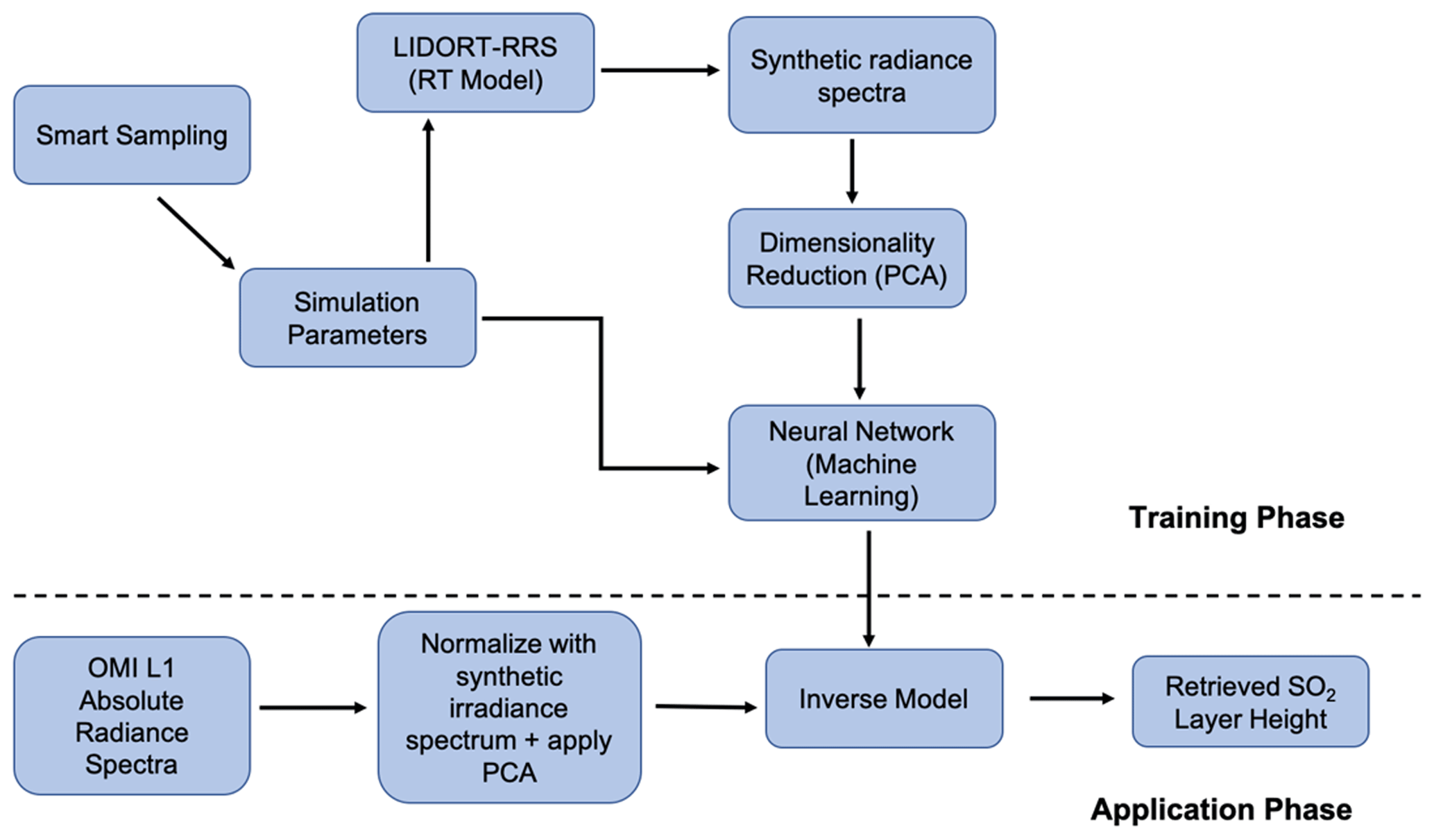
Figure 1 The flowchart of the FP_ILM methodology for retrieving OMI SO₂ effective layer height. The steps above the dashed line are part of the training phase done prior to incorporation of OMI measurements. The application phase involves deployment of the trained model to the OMI radiance measurements to obtain estimates of effective volcanic SO₂ layer heights.

2.1 Forward radiative transfer model

The first step in the training phase is to build a large dataset of synthetic backscattered Earthshine reflectance spectra from forward radiative transfer (RT) calculations. These calculations are performed using the LInearized Discrete Ordinate Radiative Transfer (LIDORT) model with rotational Raman scattering (RRS) capability (Spurr et al., 2008). This version of the model treats first-order inelastic Raman scattering in addition to all orders of elastic (Rayleigh) scattering processes. Rotational Raman scattering occurs when a photon is scattered at lower or higher energy levels than the incident radiation. RRS cannot be neglected; it is known to be responsible for the Ring effect (Grainger and Ring, 1962), a spectral interference signature characterized by the filling-in of Fraunhofer lines and telluric-absorber features. Allowing for RRS in the RT model leads to differences in calculated radiances compared to those made with purely elastic scattering, as characterized by the filling-in factor. This quantity is generally of the order of a few percent, consistent with estimates that 4 % of the total scattering in the atmospheric is inelastic (Young, 1981). Fundamentally the SO₂ layer height information can be retrieved by backscattered radiance spectra because the amount of scattering occurring in the overlying atmosphere is determined by the height of the volcanic SO₂ plume. This is demonstrated by comparing two otherwise identical RT calculations with different SO₂ layer heights (Fig. 2a). At shorter wavelengths at which Rayleigh scattering is stronger, there is less backscattered radiance for the case with higher SO₂ plume height, particularly at shorter wavelengths <320 nm (Fig. 2b). Likewise, the filling-in factor (Fig. 2c) shows the importance of including RRS in the RT calculations as in some cases there can be 2 %–3 % difference between the Raman and elastic calculations.

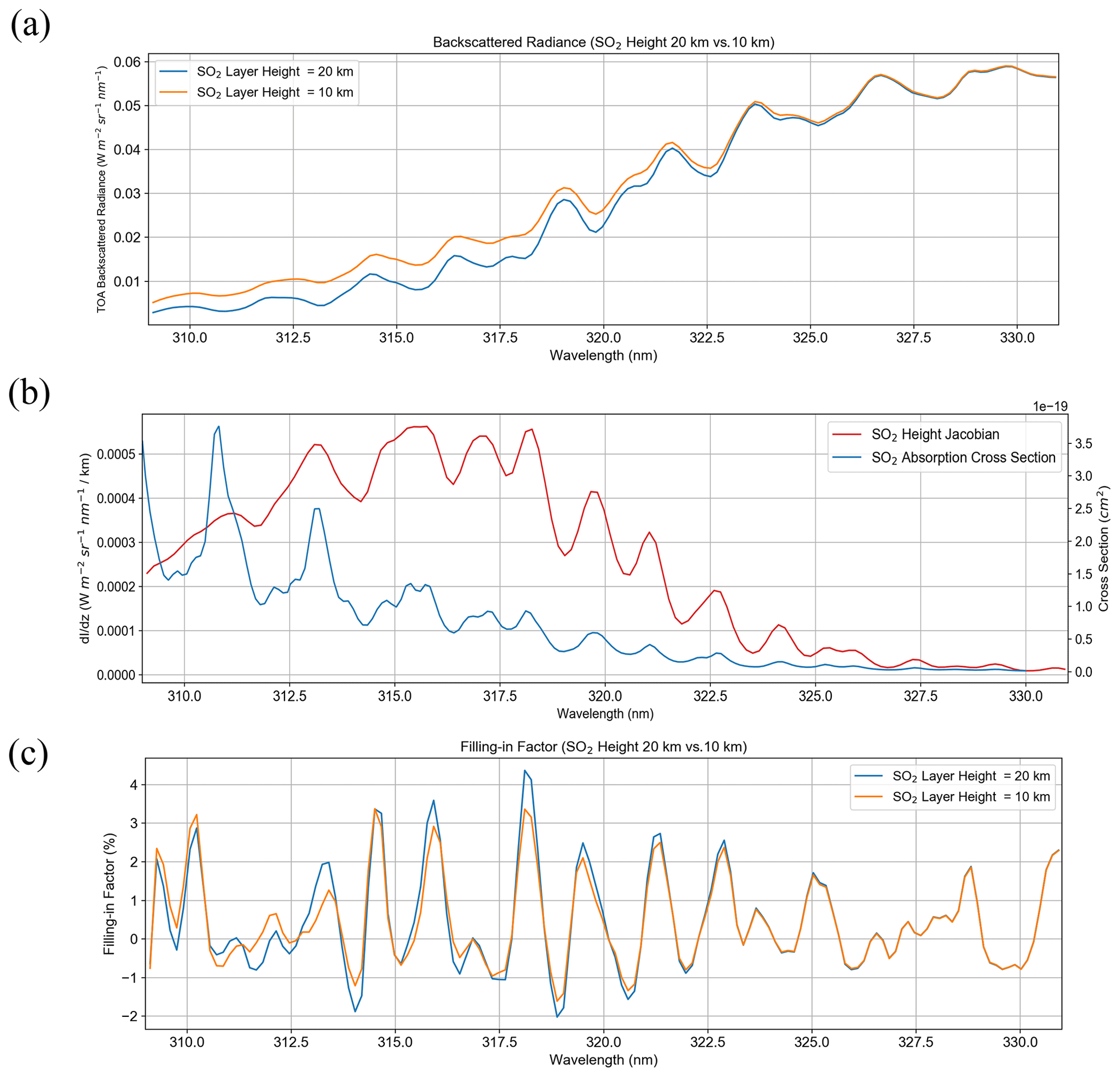
Figure 2 (a) Simulated top-of-the-atmosphere (TOA) Earthshine radiances for two different SO₂ layer heights (10 and 20 km) from the LIDORT-RRS model. Also shown: (b) the SO₂ height Jacobian (change in radiance per kilometer between the two spectra) along with the absorption cross sections of SO₂ for reference; (c) the filling-in factor. The filling-in factor is defined as the difference between the total and elastic-only radiance results divided by the total radiance and expressed as a percentage. An SO₂ column amount of 200 DU was used in the two calculations, and all other parameters were kept constant except for the SO₂ layer height.

All LIDORT-RRS calculations in this study were performed for the 310–330 nm spectral range, which captures strong SO₂ and ozone absorption features. The model is supplied with ozone (Daumont et al., 1992) and SO₂ absorption (Bogumil et al., 2003) cross sections, an atmospheric profile, an ozone profile, and a high-resolution Fraunhofer solar irradiance spectrum. The atmospheric profile has 48 layers and contains a temperature–pressure–height grid from the standard US atmosphere, with an increased vertical resolution of 0.5 km below 12 km. The ozone profile is determined by the total column amount, latitude zone, and month as specified in the TOMS V7 ozone profile climatology (Bhartia, 2002), while the SO₂ profile is assumed to be a Gaussian shape with a full-width half-maximum (FWHM) of 2.5 km. The solar spectrum is a re-gridded version of the high-resolution synthetic solar reference spectrum (Chance and Kurucz, 2010), originally with a spectral resolution of 0.01 nm. The re-gridded version has a resolution of 0.05 nm, which is finer than that for OMI (0.16 nm sampling for a FWHM spectral resolution of ∼0.5 nm). The advantage of using this reference spectrum over the instrument-measured irradiance is that only one set of calculations is needed; they can be applied to multiple instruments and instrument cross-track positions without utilizing unique measured solar flux spectra for each situation. Using instrument-measured solar flux data may carry less potential error and be able to better handle issues with instrument degradation. However, the downside is that the inverse model would need to be re-trained whenever a new measured solar flux spectrum is used. Since we expect the retrieval to be primarily sensitive to SO₂ absorption signatures, the radiative transfer calculation was performed for a molecular atmosphere with no aerosol scattering.

In order to obtain a large number of different spectra, eight key physical parameters were varied for the LRRS calculations. These parameters include solar zenith angle (SZA), relative azimuth angle (RAA), viewing zenith angle (VZA), surface albedo, surface pressure, O₃ column amount, SO₂ column amount, and SO₂ layer height. The ranges of these parameters are given in Table 1.

Table 1 Ranges of the eight physical parameters varied in LIDORT-RRS for the synthetic spectra calculations.

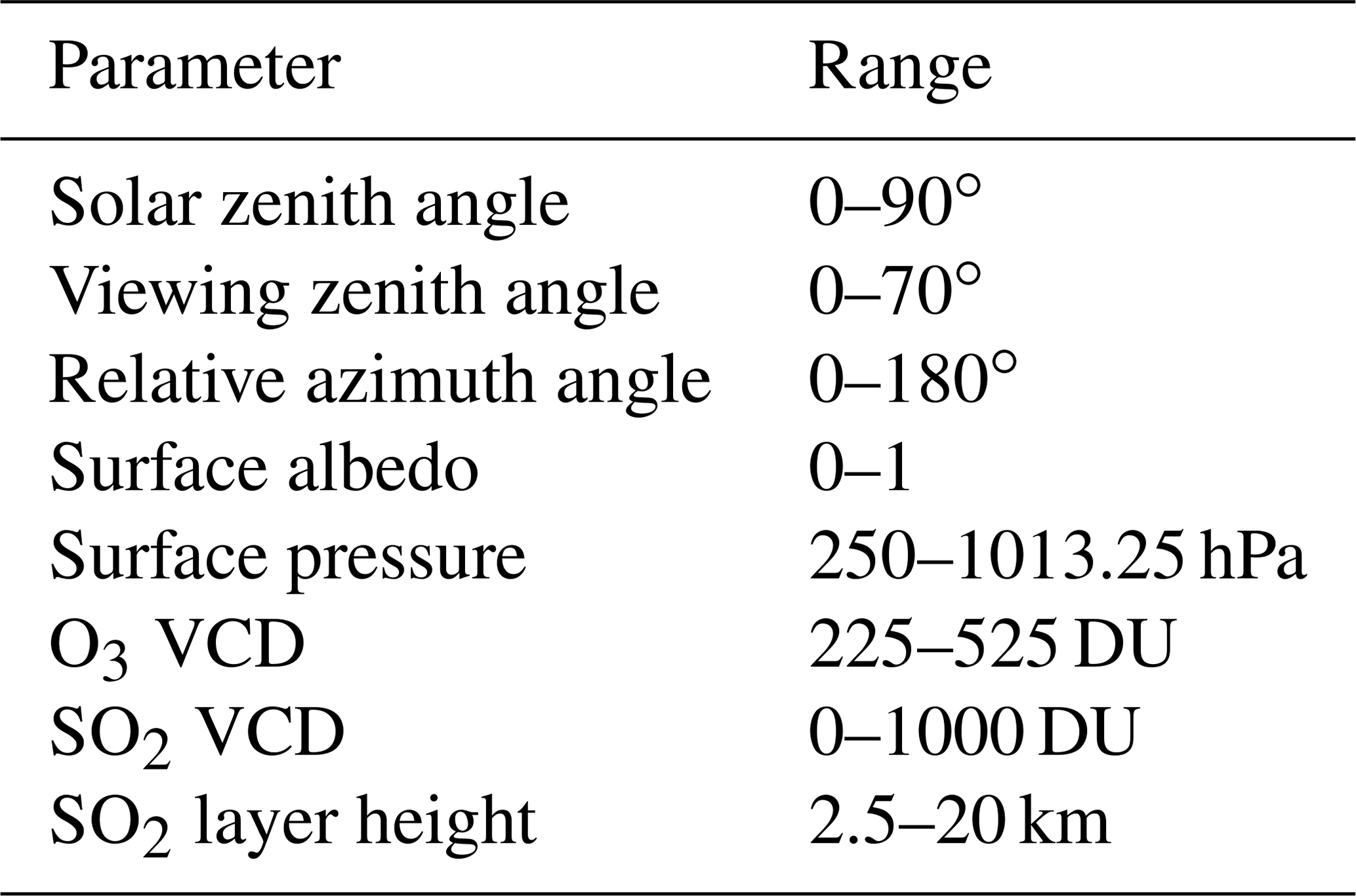
The number of calculations and the parameter sets for each simulation were determined through a smart sampling technique (Loyola et al., 2016). A selective parameter grid with sets of parameters for each simulation was established through the use of Halton sequences (Halton, 1960) in eight dimensions. The calculations are continued until the moments of the output data, mean, and median converged across all wavelengths. In total around 200 000 calculations were done to achieve a sufficiently comprehensive sample size for the variation in the eight parameters across all rows of OMI. This sampling was done in order to ensure that (1) each set of parameters was unique and training data are diverse, and (2) the sample size of the entire dataset is large enough for the machine-learning application.

2.2 Data pre-processing

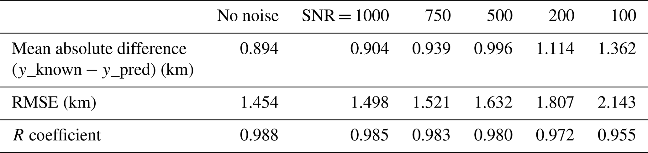
After the RT calculations are completed, the spectra are convolved with the OMI slit function. Since each cross-track position of OMI contains a unique slit function, the appropriate function was applied based on the VZA input for that particular calculation. The VZA ranges from 0–70^∘ across all rows in the OMI swath, with the middle (nadir) rows having a VZA of close to 0. For each row, only spectra within ±3^∘ of the actual VZA were convolved with the appropriate slit functions. In addition, Gaussian noise with a signal-to-noise ratio (SNR) of 1000 was added to the spectra. While the SNR of OMI tends to be lower (Schenkeveld et al., 2017), adding too much noise can greatly decrease the performance of the machine learning (Table 2). The root mean squared error (RMSE) and mean absolute difference (MAE) between the SO₂ height from the RT calculation parameter sets and the height predicted by the neural network were used as metrics (see Sect. 3). At SNRs of less than 500, the performance starts to increasingly degrade. Between SNRs of 1000 and 500, there is an increase of around 0.1 km in RMSE. However, adding some degree of noise is necessary to account for errors in satellite instrument measurements.

Table 2 The RMSE and the mean absolute difference (km) of all data points in the independent test set after adding noise as indicated by different SNR values. All other parameters and input data were kept constant. SZA < 75^∘ and SO₂ VCD > 40 DU were excluded from the test set for these comparisons.

Next, principal component analysis (PCA) was applied to the spectral dataset for each row in order to extract the most significant features of the spectra and to reduce dimensionality. Since each convolved sample consists of 142 wavelength points, the dimensionality of this problem becomes very large. However, PCA transforms each sample to a set of weights based on eight principal components (PCs). These principal components explain 99.998 % of the variance in the synthetic dataset (Fig. 3). Including additional PCs does not add any significant value to the retrieval and may even lead to overfitting. Prior to starting the machine-learning process, the dataset is split into a training subset (90 %) and a testing subset (10 %). The training subset is used for the neural network learning, while the testing subset is only deployed to verify the performance of the network to predict the output.

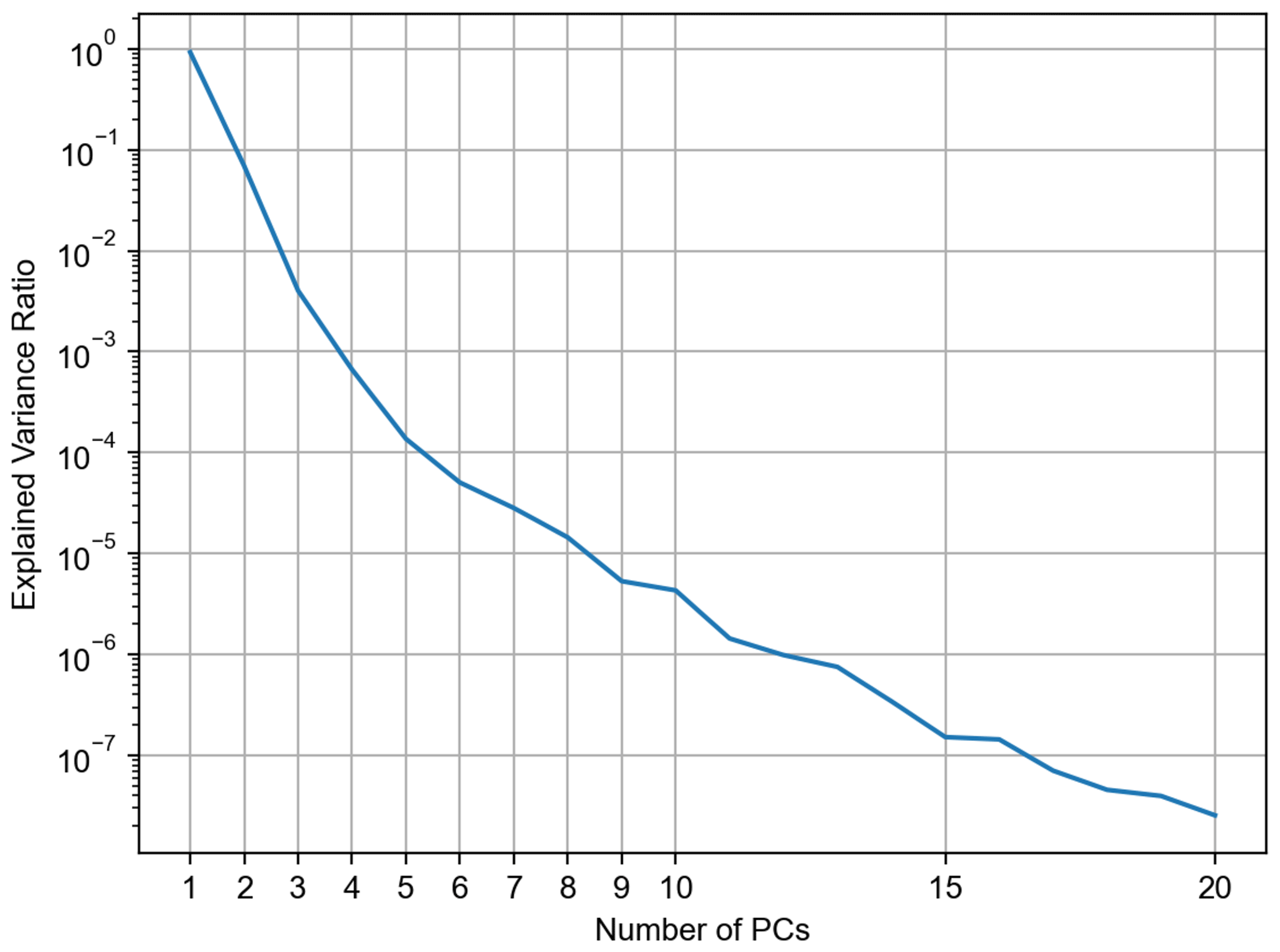
Figure 3 Explained variance ratio as a function of the number of principal components of the spectral dataset.

2.3 Machine learning using a neural network

The eight PCs and selected parameters including the SZA, RAA, VZA, surface pressure, and surface albedo were used as input for training an MLPR, which is sometimes referred to as a deep neural network. The output layer of the NN contains the effective SO₂ layer height. Column amounts of SO₂ and O₃ were not included in the training or in the application stage because of the large dependency of column amounts on SO₂ layer height and due to biases in OMI ozone retrieval in the presence of the enhanced SO₂ plume, respectively. To improve stability, the inputs (PC weights, SZA, VZA, etc.) and output (effective SO₂ height) are scaled between −0.9 and 0.9 according to the minimum and maximum of each input variable prior to input into the NN. In an NN, the input and output layers are connected by hidden layers containing neurons (also known as nodes). Each neuron is connected to others by a series of weights, by means of which the input data are passed to the next level as a weighted sum of all inputs. Inside the neural network, the Adam optimizer with a stochastic gradient descent algorithm (Kingma and Ba, 2015) is used to minimize the loss function, in this case the mean squared error (MSE) between the result of each iteration and the actual SO₂ layer height used to generate the synthetic spectral sample. With each iteration, the partial derivative of the MSE with respect to each node is calculated; this is used to update the weights. The training of an NN progresses by cycling through iterations of the entire training dataset, called epochs, until the training and validation MSE is minimized and there is no improvement to be obtained from further training. Throughout the training, the NN uses 10 % of the training subset for validation to assess the performance with each iteration. This validation set is different from the independent test data that were set aside from training. The “tanh” (hyperbolic tangent) activation function is applied at the hidden layers to further increase stability in the NN. Other activation functions (e.g., ReLU and PReLU) were tested; however, tanh was found to produce slightly better NN performance. There is also considerable flexibility in the structure of the NN, in particular the number of hidden layers and nodes in each layer. The final configuration of the NN in this study includes two hidden layers with 20 and 10 nodes in the first and second layer, respectively. This was determined through testing and analyzing the errors of the NN with respect to the synthetic test dataset and the quality of the retrieval results after application to satellite measurements. More complex configurations of hidden layers and numbers of neurons were also tested and found to have worse performance when using OMI data as input. Hence, the relatively simple configuration was chosen as the final setup for this study.

In neural networks a common problem known as overfitting often occurs when the machine-learning model is tuned so closely to the training inputs that it does not perform well on new data. During training this can be diagnosed if the validation error is much higher than the training error. To reduce overfitting, L2 regularization was implemented in the training. The regularization reduces the effect of small and very large weight values by penalizing the MSE loss function. For this study, the training was done separately for each OMI row due to the different VZAs and slit functions between rows; however, the configuration of the NN was kept constant between rows. The only difference in the training is the number of training epochs conducted for each row before the solution becomes optimal for that row. The number of epochs varies slightly but is in the 200–300 range for all rows. The final trained version of the NN, the inverse operator, contains the optimal weights needed to predict the SO₂ layer height from an input of separate test data.

An important aspect for neural network performance is the number of training samples. Aside from smart sampling, the appropriate number of samples for training can be determined by comparing errors from training runs wherein different percentages of training samples were removed (e.g., 10 %, 20 %, 50 %) beforehand. The mean absolute error between height predicted by the NN and the test set height was calculated when using different numbers of input samples. With a 50 % reduction in training samples, the absolute error went up by around 0.3 km. In contrast, reducing the training set by 10 % had little impact on the error (see Table A1). These results provide confirmation that for this case the training data are adequate and that there would likely be diminishing returns in NN performance with a larger training dataset.

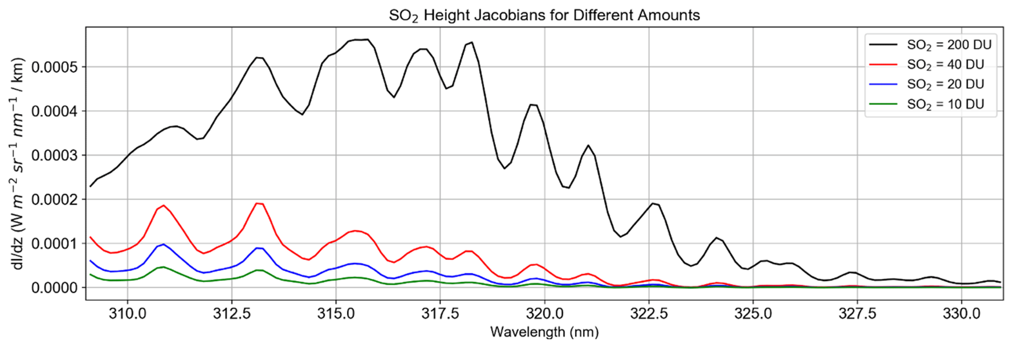
Figure 4 SO₂ Height Jacobians ($\mathrm{d}I/\mathrm{d}z$) for four different assumed SO₂ column amounts. The Jacobians were calculated from the difference between two radiance spectra with 10 and 20 km SO₂ height. All other physical parameters were identical in the calculation of the spectra.

2.4 Application to satellite measurements

In the application phase of the retrieval, the inverse operator is applied to OMI radiance spectra, resulting in a predicted SO₂ layer height for each ground pixel in the OMI swath. For this the OMI L1B geolocated Earthshine radiance dataset is used. Since OMI only provides absolute radiances, these data were normalized with respect to the same solar flux spectrum as used in the generation of the synthetic spectra. In other words, the measured input becomes the fraction of backscattered radiance to the incoming solar irradiance (i.e., reflectance spectrum). Prior to normalizing, the irradiance spectrum was convolved with an OMI slit function for the particular OMI row and orbit. The irradiance spectrum is convolved with the appropriate OMI slit function in order to have consistency in wavelength points between the measured radiances, synthetic radiances, and irradiance of each row. To follow the same procedure as was used in the training step, the PCA operator from the training phase is applied to the OMI spectra to perform the dimensionality reduction and obtain a set of PC weights for each sample. The other inputs are VZA, SZA, RAA, albedo, and surface pressure parameters from the OMI data files. As in the training phase, all inputs are scaled to the [−0.9, 0.9] range. After SO₂ heights are retrieved separately for each row, one height value is given for each pixel (and spectral sample). The application phase of the retrieval takes only 2–3 s for a given row. This short duration includes the application of the training phase PCA operator to OMI measurements, the scaling of inputs, and the deployment of the inverse operator. The whole process is repeated for each row in order to get a prediction for an entire OMI swath. For some rows the retrieval is unreliable due to the row anomaly, which negatively affects the quality of the OMI L1B radiance data at all wavelengths and consequently L2 retrievals.

3 Impacts of various parameters on the performance of the trained inverse model

From the training phase, it becomes clear that the performance of the algorithm will depend on several factors. As demonstrated in Fig. 3, an important factor is the SO₂ column amount. Overall, the NN makes better predictions for the test data subset for SO₂ amounts >40 DU. Below 40 DU, information content on the layer height to be retrieved becomes increasingly small, as evidenced by large differences between predicted heights and those in the actual test set (Fig. 5a). Additionally, larger SO₂ loadings result in greater sensitivity between two heights, as seen by comparisons of SO₂ height Jacobians for multiple amounts (Fig. 4). Quantitatively, if samples with SO₂ amounts less than 40 DU are excluded, the RMSE decreases from 1.48 to 1.15 km (Table 3). As with other sensitivity analyses, the RMSE and MAE in Table 3 are calculated between the predicted output from NN and the height from the independent test dataset. We can therefore expect the retrieval to produce reasonable results for moderate to large volcanic eruptions. In widely dispersed plumes wherein the SO₂ VCD is low or for volcanic degassing events, the retrieval would be less accurate. The second major dependency is on SZA. The problem here stems from the occurrence of relatively large errors in RT modeling due to shallow light paths and lower OMI SNR at the higher SZAs. Reasonably accurate results are to be expected only for SZA < 75^∘. Figure 2b shows significant differences in predicted and actual heights in spectra associated with large SZAs after removal of low VCD samples. For the final training approach, it was therefore necessary to exclude spectra with large SZAs. Dependencies on other physical parameters are small when compared with these two issues discussed here, although there is some evidence that high surface albedo also increases error. If we remove spectra with albedo >0.6 there is a minor improvement in RMSE from 0.93 to ∼0.89 km. However, even with strong volcanic SO₂ signals, we can realistically expect the absolute error to be at least 1 km on average due to inherent simplifications in the neural network retrieval approach. The errors in actual retrievals using OMI data are expected to be larger (see Sect. 4.4).

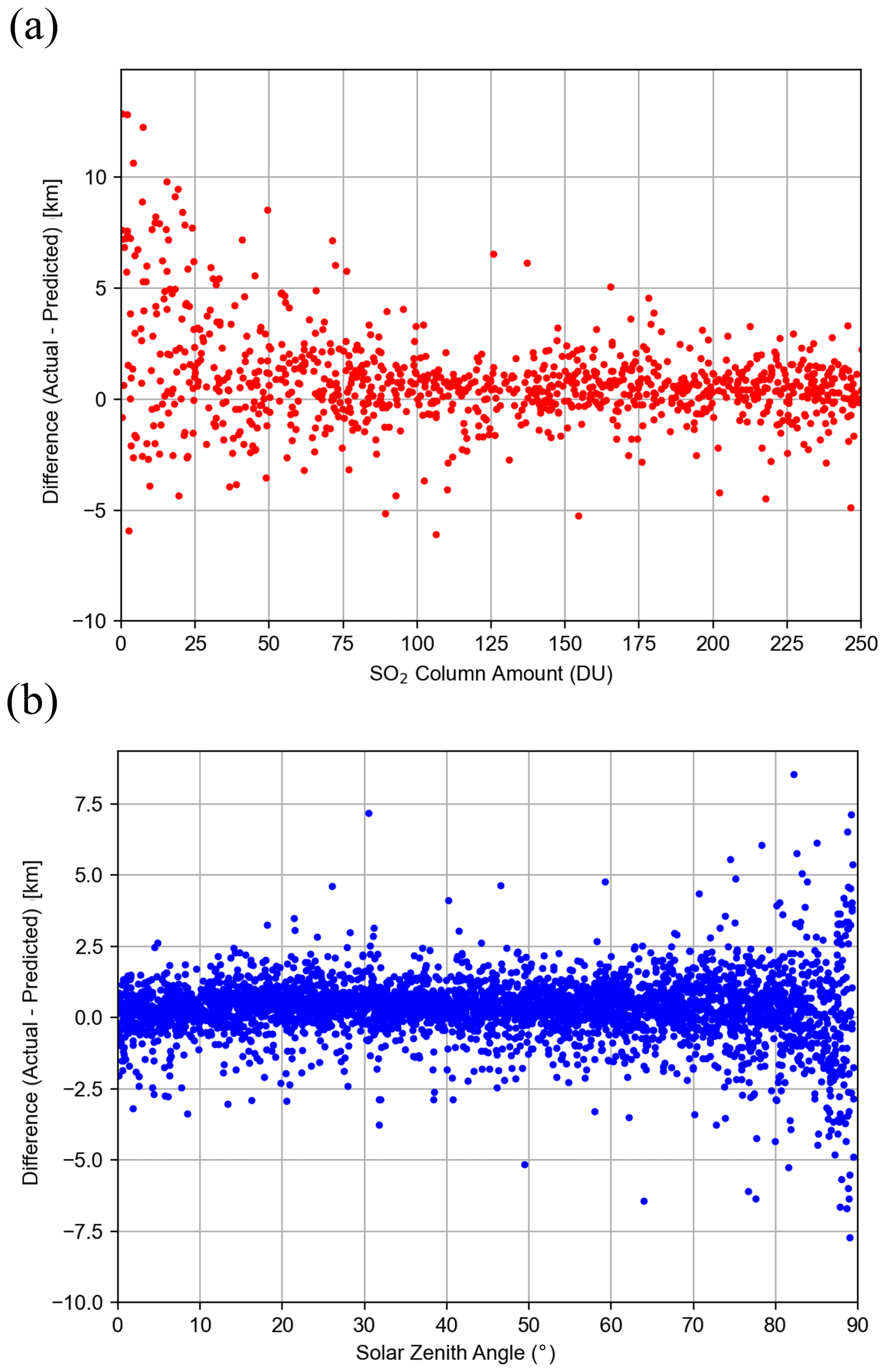
Figure 5 Dependence of retrieval errors on (a) SO₂ amount and (b) SZA for cases with SO₂ VCD > 40 DU. The error is defined as the difference between the SO₂ layer height predicted by the neural network using inputs from the independent test set and the actual height from the same samples. The test set comprises 10 % of the original spectral dataset withheld from training the neural network. The plots show that the retrieval error is mostly within ±2.5 km for SZA < 70, but it increases significantly for large SZAs.

Table 3 The RMSE and the mean absolute difference of all data points in the test set under different conditions. For each condition, the appropriate points were removed and excluded in error calculations. All cases in this table used synthetic training spectra with added SNR 1000.

4 OMI SO₂ effective layer height results

For testing the FP_ILM retrieval on OMI data, four volcanic eruption cases with sufficiently strong SO₂ signals were selected (i.e., with peak SO₂ VCDs greater than 40 DU). Each case is described in detail in the following subsections. For each case, comparisons were made to other satellite-derived datasets where available, for example the CALIOP lidar on board CALIPSO, the IASI SO₂ layer height retrieval (Clarisse et al., 2014), and the GOME-2 (Efremenko et al., 2017) and TROPOMI retrievals (Hedelt et al., 2019). It is important to note that the CALIOP lidar only indicates the height of the ash plume and not the SO₂ height. Although ash and SO₂ plumes are often collocated, this is not always the case, making direct comparisons difficult.

4.1 Kasatochi (2008)

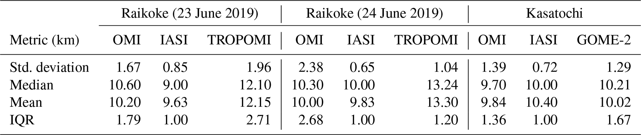
Kasatochi is a volcano located on the Aleutian Islands of Alaska (52.178^∘ N, 175.508^∘ W). It underwent a series of eruptions beginning late in the day on 7 August 2008, which injected great amounts of ash and SO₂ into the stratosphere. Overall the explosion released roughly 2 million tons of SO₂, at the time the highest SO₂ loading since the Mt. Pinatubo eruption (Yang et al., 2010). SO₂ effective layer heights retrieved using the machine-learning model for OMI (orbit 21650) on 10 August 2008 were around 11–12 km, with some portions being slightly lower (Fig. 6a). This is in reasonable agreement with previous SO₂ height retrievals of 9–11 km that used the ISF algorithm for OMI (Yang et al., 2010) considering that the uncertainty of both retrievals is around 2 km. Likewise, Nowlan et al. (2011) showed that the majority of the plume was around 10 km and up to 15 km in some parts. There is also agreement with IASI (Fig. 6b) and CALIOP data (Fig. 6d), which showed plume heights of 10–12 and 12.5 km, respectively. It is important to note that the IASI overpass occurred later in the day than those for OMI and CALIPSO. Another verification source we used was the GOME-2 SO₂ layer height retrieval that uses FP_ILM (Efremenko et al., 2017). The study found a height of around 10 and up to 14 km in areas of high SO₂ loading for 10 August (Fig. 6c). The GOME-2 overpass occurred 4 h earlier than OMI. The mean, median, standard deviation, and inner quartile range (IQR) of the three retrievals (Table 4) also show good agreement for this case. Although the OMI results agree well in general with the results of these studies and datasets, the retrieval is less sensitive with respect to detecting variability in the SO₂ layer height within the plume.

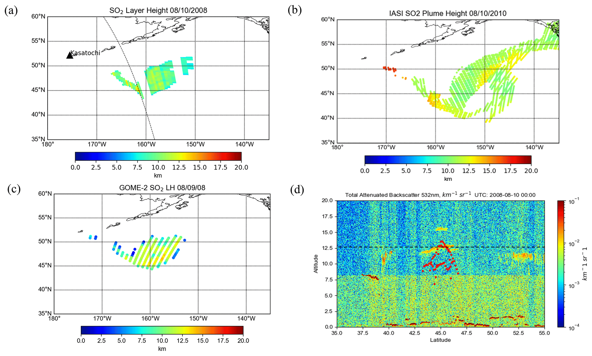
Figure 6 Comparison between the volcanic plume heights from (a) OMI, (b) IASI, (c) GOME-2, and (d) CALIOP lidar 532 nm attenuated backscatter for the 2008 Kasatochi eruption. The black dotted line in (a) shows the CALIPSO track. Some rows of OMI in this case were affected by the row anomaly, as seen by the gaps in the plume. The red dots in (d) show the OMI retrieval near the CALIPSO path, and the black dashed line denotes the height of the ash plume observed by CALIPSO.

Table 4 Statistical comparisons of the SO₂ height retrievals for 2 d of the Raikoke eruption and the Kasatochi eruption cases.

4.2 Kelud (2014)

Kelud, a stratovolcano located in East Java, Indonesia (7.935^∘ S, 112.315^∘ E), erupted on 13 February 2014 at 15:50 UTC, in the process depositing ash in a 500 km diameter around the volcano and leading to mass evacuations from nearby towns. Even though this case has somewhat lower SO₂ VCDs than those from Raikoke and Kasatochi (see Fig. A1), the peak SO₂ VCDs of ∼60–70 DU should still allow for retrievals with reasonable accuracy (see Sect. 2). The OMI retrieval results indicate that the maximum height of the main plume was 18–19 km (Fig. 7a), although other studies suggest that several smaller layers of SO₂ and ash were located as high as 26 km (Vernier et al., 2016) on the previous day. However, the SO₂ loading at that level was most likely too low for an accurate retrieval using OMI radiances. CALIOP lidar detected ash plumes at around 19.5 km, and the IASI retrievals registered the plume at 17.5 km over the same area as that for OMI. The height of the ash plume from this eruption was also estimated using Multifunctional Transport Satellite (MTSAT 2) observations and transport modeling (Kristiansen et al., 2015). That study found an injected height of around 17 km, which is in agreement with the OMI result, especially when considering the most probable heights on the probability density function (PDF) (Fig. 8b). We note here that only a small portion of the plume was retrieved with our algorithm given the relatively low SO₂ VCDs and interference due to the OMI row anomaly. It is promising to note that the OMI retrieval was able to identify heights at the upper end of the height range used in the training phase. On the other hand, while the retrieval can extrapolate to heights above 20 km, the accuracy would likely degrade due to the lack of training data with heights outside this limit.

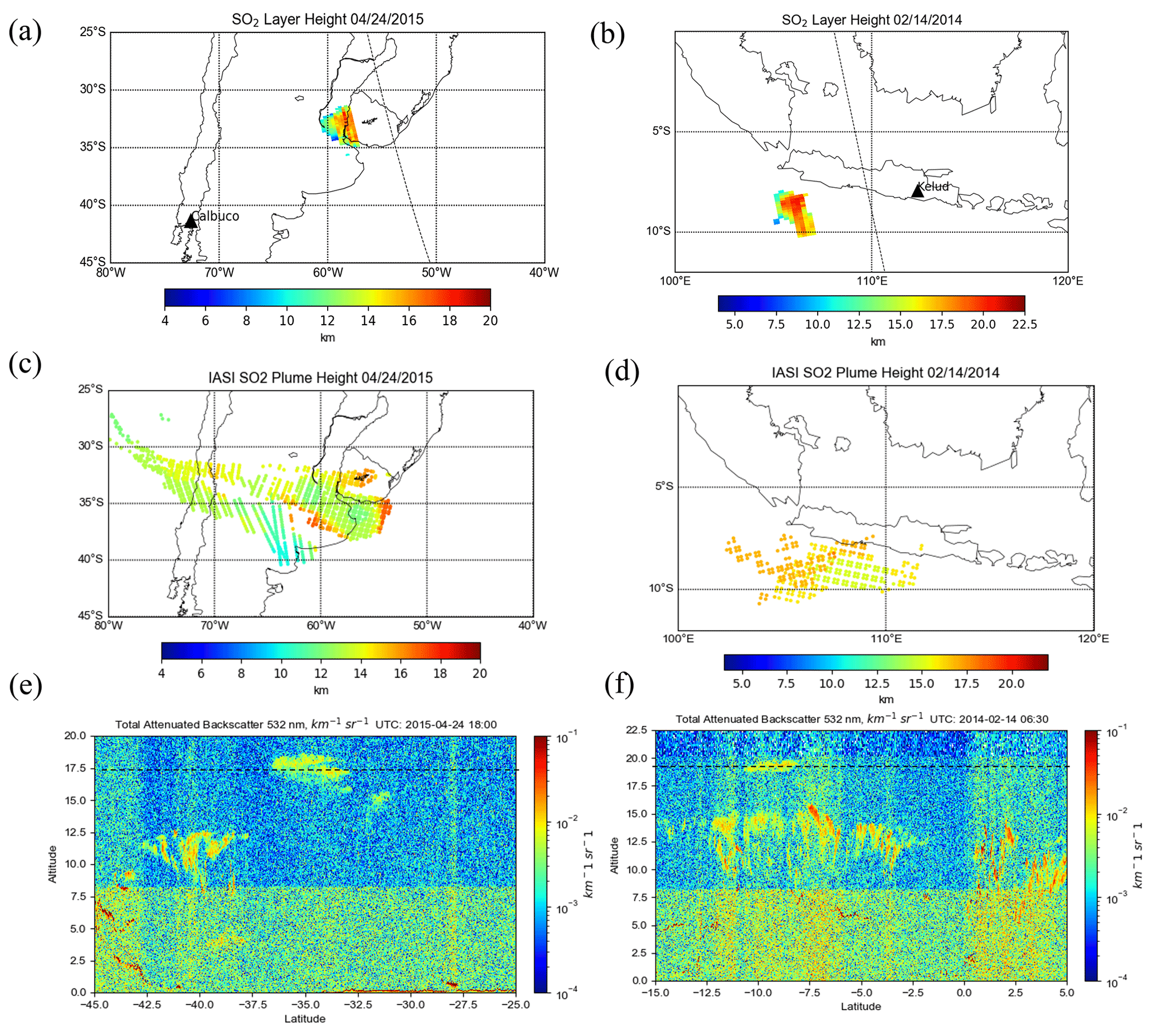
Figure 7 Comparisons of plume heights for the 2015 Calbuco eruption (a, c, e) and the Kelud eruption (b, d, f) for OMI (a, b), IASI (c, d), and 532 nm total attenuated backscatter from the CALIOP lidar (e, f). For OMI, only pixels with >30 DU of SO₂ are shown, and retrievals were unavailable for some parts of the plume due to the row anomaly. The black dotted line in (a) and (b) marks the CALIPSO track. The white rectangles in (e) and (f) show the location of the plume in the lidar profile. Direct comparison with CALIPSO was not possible due to obstruction by the OMI row anomaly.

Figure 8 Probability histograms of SO₂ effective layer height retrievals for (a) the Calbuco eruption on 24 April 2015 and (b) the Kelud eruption on 14 February 2014.

4.3 Calbuco (2015)

The Calbuco volcano is located in Chile (41.331^∘ S, 72.609^∘ W). The primary eruption had a volcanic explosivity index (VEI) of 4 and occurred on 22 April with little warning. The primary plume ascended higher than 15 km, while plumes from smaller subsequent eruptions stayed in the troposphere. The volcanic plume spread northeast in the following days, resulting in flight cancelations at Uruguayan and southern Brazilian airports. The OMI-retrieved SO₂ effective layer heights in the area of greatest VCD was in the 15–17 km range. In the same region, IASI results (Fig. 7c) show similar plume heights of approximately 15 km, although as with the previous events, the overpass times of the two instruments are different. CALIOP lidar shows the ash plume at roughly 17 km (Fig. 7e). Unfortunately, the overpass of CALIPSO occurs over an area of OMI's swath that is affected by the row anomaly, and this makes a direct comparison unfeasible. Nevertheless, the CALIPSO aerosol layer height is still comparable to OMI-retrieved effective SO₂ layer heights for the portion of the plume further to the west. The retrieval for OMI is consistent with the other instruments for SO₂ plumes, with the exception of the part of the plume with SO₂ below 30–40 DU (see Fig. A1), for which results were not plotted in Fig. 7a due to lower biases.

4.4 Raikoke (2019)

The eruption of the Raikoke stratovolcano (48.2932^∘ N, 153.254^∘ E), located on the Kuril Islands of Russia, occurred on 21 June 2019 at 18:00 UTC. A series of explosions during the eruption sent large amounts of ash and SO₂ into the lower stratosphere. Maximal loadings of SO₂ measured by OMI and other sensors exceeded 500 DU. In the following days the plume underwent dispersion and spread out over the northern Pacific Ocean and later over eastern Russia. Early estimates of plume injection height for the eruption were predominantly in the 10–13 km range, with potentially larger heights in some areas of the plume. In Fig. 9a and b, the SO₂ effective layer heights retrieved from OMI data are shown for the Raikoke plume on 23 and 24 June, respectively. The plume heights for both days are predominantly in the range 10–12 km, although some areas of the plume had estimated peak heights of 13–14 km. In comparison, the TROPOMI results show slightly larger heights (13–14 km) for 24 June and similar heights as OMI for 23 June (Fig. 9c and d). The IASI SO₂ height product also shows fairly good agreement, with heights mainly at the 10–11 km level (Fig. 9e and f). It is also useful to look at a distribution of heights predicted for the domain (Fig. 10) in order to get a more quantitative comparison between the datasets. Based on this distribution, there is clearly at least 2 km of difference between the most probable heights from OMI and those from TROPOMI for 24 June (Fig. 10b and d) and slightly lower heights in the distribution for IASI. This is also displayed in Table 4, which shows a 2–3 km difference in the mean and median of retrieved heights between OMI and TROPOMI. Additionally, the IQR and standard deviation provide a quantitative measure of the variation in the distribution of the retrieved heights, which can change from one orbit to another. Note that points with values lower than 30 DU are not included in the PDFs for all sensors. The results are also compared with the CALIOP lidar on board CALIPSO, which shows ash plume heights of 12–13 km for both days (Fig. 11a and b). Although there is overestimation for some OMI pixels, especially for 24 June, the section of the plume with the CALIPSO flyover has similar heights (around 12.5 km) as lidar-determined aerosol layer altitudes. Lastly, we note that a recent study highlighted probabilistic height retrievals using the Cross-track Infrared Sounder (CrIS) for Raikoke. This study found a median height of 10–12 km across a large part of the plume but with some areas upwards of 15 km. While there are some notable differences across all of the datasets, the OMI retrieval for this case falls within the general consensus of plume height estimates for this volcanic event.

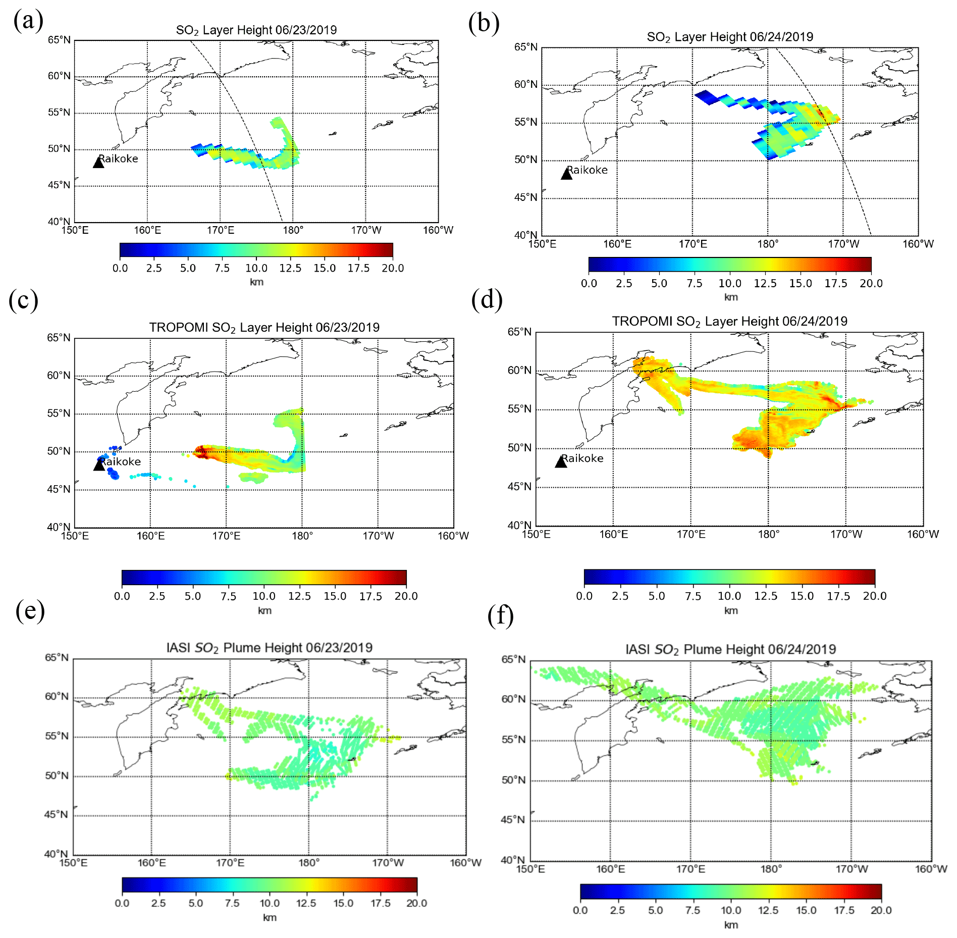
Figure 9 The SO₂ layer height retrieval for the Raikoke eruption plume on 23 June 2019 (a, c, e) and 24 June 2019 (b, d, f) for OMI (a, b), TROPOMI (c, d), and IASI (e, f). For all three sensors, only pixels for which SO₂ VCD > 30 DU are shown.

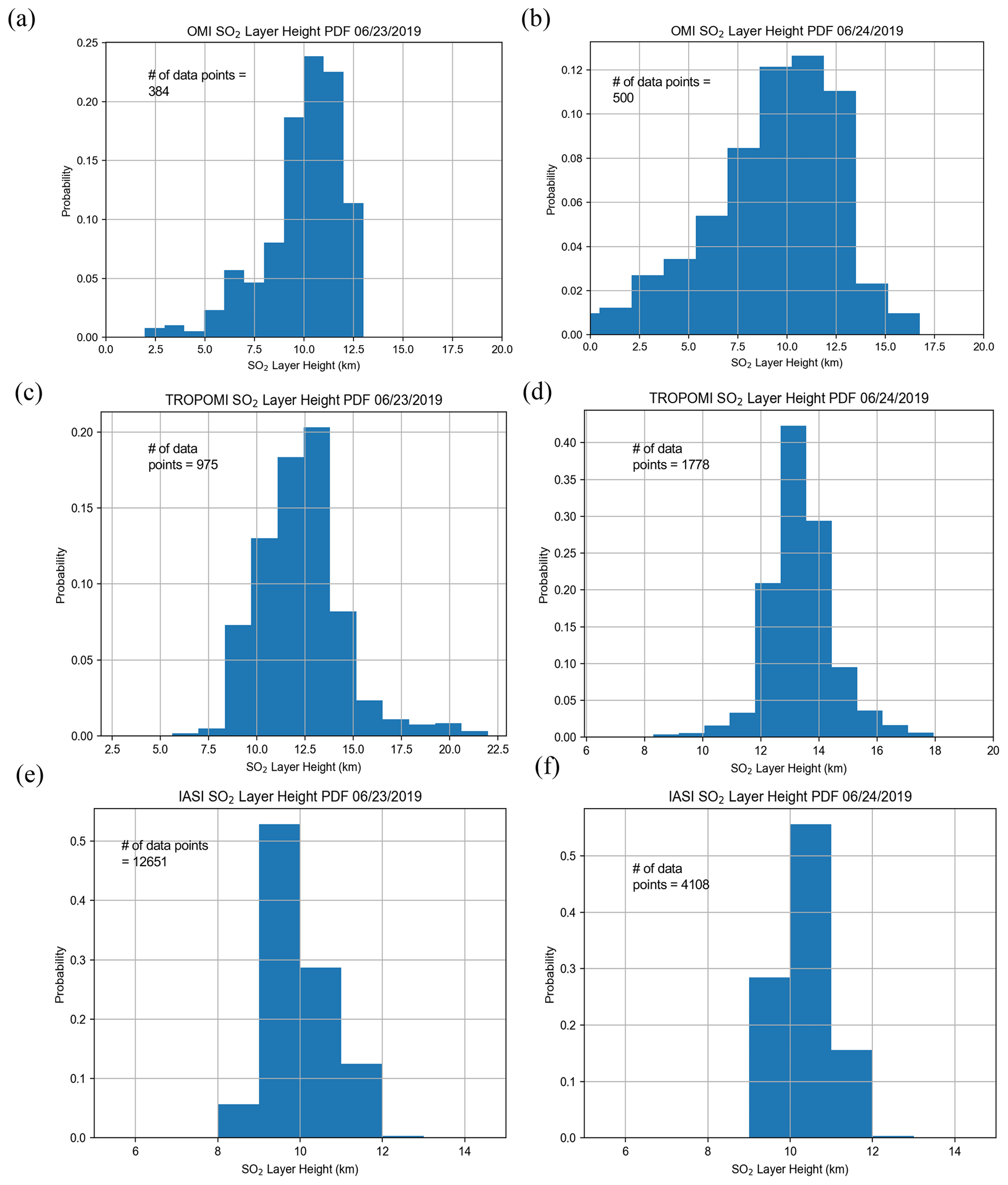
Figure 10 Probability histograms of SO₂ layer height retrievals for (a, b) OMI, (c, d), TROPOMI, and (e, f) IASI on 23 June 2019 (a, c, e) and 24 June 2019 (b, d, f). Only pixels with an SO₂ column amount greater than 30 DU are included. These plots correspond to the results plotted in Fig. 4a–f.

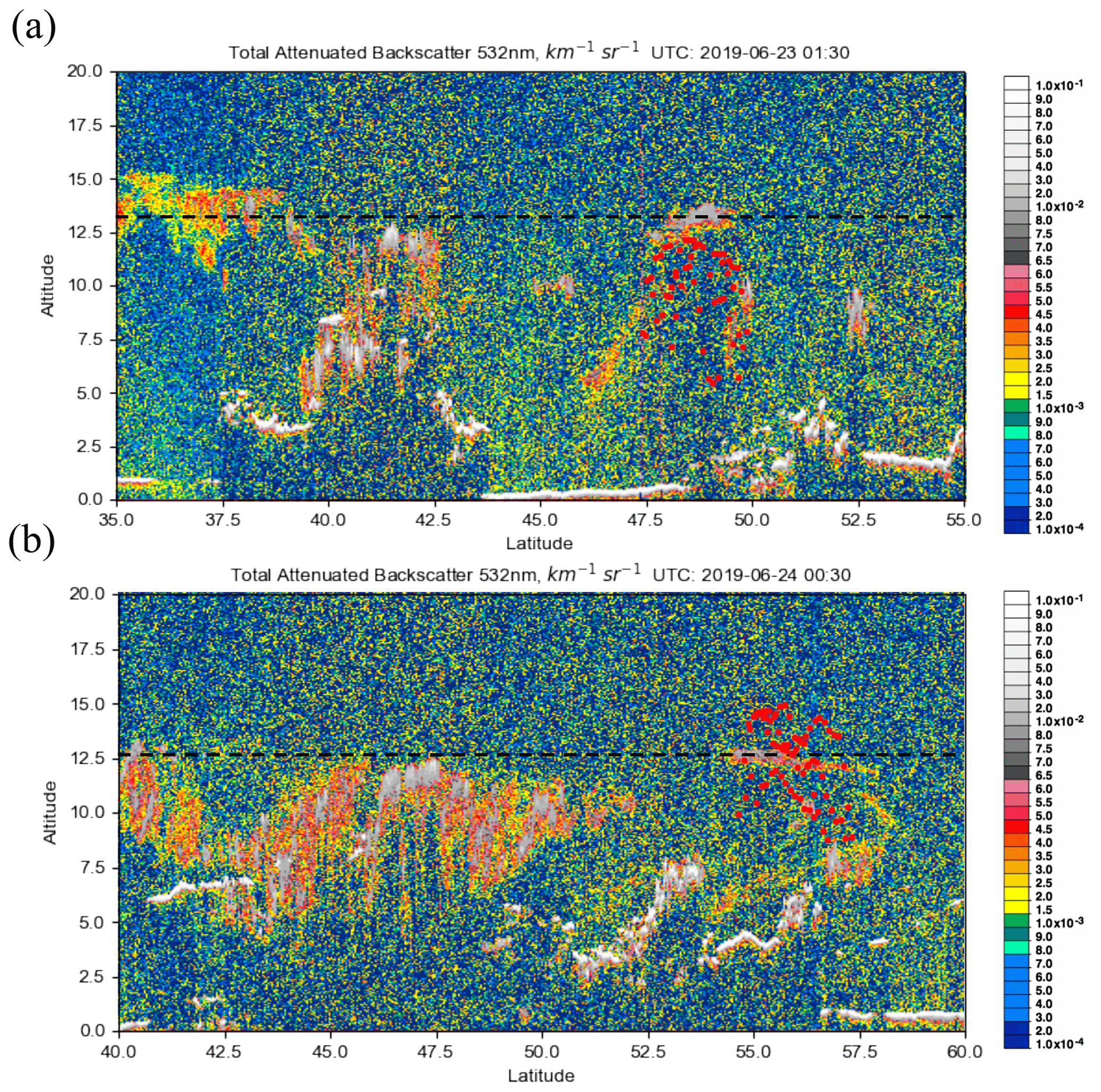
Figure 11 CALIPSO lidar 532 nm attenuated backscatter for the Raikoke eruption on (a) 23 June and (b) 24 June 2019. The black dashed line symbolizes the height of the ash plume seen by CALIPSO, and red dots show the results from the OMI retrieval along CALIPSO's flight path. The flyovers occurred shortly after 01:30 and 00:30 UTC on 23 and 24 June, respectively, around the same time as OMI.

4.5 Discussion of errors

It is clear that predicting SO₂ layer height with FP_ILM is an efficient process, but one that is not flawless in terms of accuracy. As comparisons between instruments and retrievals have shown, on average there were 1–2 km differences in heights, especially for the Raikoke event, although we consider this to be good agreement given the estimated MAE and RMSE associated with this retrieval. In this regard, the retrieval is an approximate estimate of the SO₂ plume height rather than a precise determination. Differences in the retrieved heights between different studies and algorithms result from differences in instruments, forward model assumptions, and retrieval techniques as well as uncertainties in each retrieval. For instance, IASI is a thermal IR instrument and its retrieval does not use FP_ILM. Therefore, exact agreement with IASI results is difficult to achieve, especially since the IASI retrieval itself has a stated error range of ±2 km, although its retrievals serve as a good verification dataset. The stated uncertainty for TROPOMI retrievals (Hedelt et al., 2019) is ∼2 km for SO₂ amounts greater than 20 DU, similar to our estimated uncertainties for OMI. While the general retrieval approach for TROPOMI (Hedelt et al., 2019) is similar to that for OMI in the present study, there are also important instrument differences that can lead to differences in the retrieved heights between the two instruments, such as the pixel size, noise, radiometric accuracy, and level of degradation. TROPOMI has a much finer spatial resolution compared to OMI, with footprints typically 5.5×3.5 km² up to a maximum size of 7×3.5 km²; TROPOMI also has larger maximal SO₂ signals. Consequently, TROPOMI is better able to resolve localized variations in the height throughout the plume and is likely to be more accurate overall due to better SNR. However, current TROPOMI L1 data are known to have issues with instrument degradation and radiometric accuracy in the UV spectral range (Ludewig et al., 2020); this could be a potential contributing factor to the differences between the two instruments. OMI retrievals show more or less uniform height levels across the entire plume, with the peak heights in areas with the best SO₂ signal. Note that CALIOP lidar profiles sometimes show disagreement with OMI-retrieved heights because CALIOP only identifies the height of the ash or aerosol plume. It also offers a comparison for only a single cross section of the entire plume per orbit. Despite the uncertainties, the consensus provided by different instrumental datasets can provide a reasonable estimate for the SO₂ layer height and, if done in near-real time, can aid in decision-making with regards to aviation safety.

Another source of error is present in the training phase. One difficulty here is finding the ideal choice of neural network setup. With many parameters to consider, such as the number of input PCs, number of layers, number of nodes, learning rate, regularization, and weight initialization, it is very time-consuming to optimize the neural network setup. We have found a relatively simply configuration that performed reasonably well with both test data and real OMI measurements for all scenarios and events considered. However, even after optimization of the parameters, random error inherently exists in the neural network. A measure of random error can be obtained by altering the random state of the neural network whilst keeping other parameters constant. For 10 trial runs with different random seeds, variations of the MAE error were around 0.15–0.2 km (see Table A2). Although the differences in the errors calculated with the synthetic test data are relatively small, larger changes can be expected during the application phase. Indeed, when applying the inverse models to OMI, there is noticeable variation of up to 1 km in the retrieved height for the same pixels. It is thus difficult to improve results further than ∼1 km of absolute error, even in the training phase. In the application phase, some additional error comes from the differences between synthetic spectra and real satellite measurements with noise errors. For example, with an SNR of 500 used in training, which is a typical noise level for OMI, the RMSE of the neural network prediction is around 1.25 km (Table 3). This can be considered the lower limit of retrieval error when the inverse operator is used on OMI measurements. Lastly, some deviations between the measured and synthetic training spectra originate from the RT modeling. The calculations contain several assumptions including the SO₂ plume shape, atmospheric profiles, gas profiles, and a molecular scattering atmosphere. Further testing is required in order to determine if the inclusion of aerosols in RT calculations would improve the algorithm performance.

5 Conclusions

In this study we have introduced a new algorithm for OMI retrievals of the volcanic SO₂ effective layer height from UV Earthshine radiances. This algorithm is based on an existing FP_ILM method that combines a computationally time-consuming training phase with full radiative transfer model simulations and a machine-learning approach to develop a fast inverse model for the extraction of plume height information from radiance spectra. Fast performance means that the algorithm can be considered for operational deployment given that the retrieval of an SO₂ layer height prediction from the inverse model takes only a matter of milliseconds for a single OMI ground pixel. For the training, a synthetic dataset of Earthshine radiance spectra was created with the LIDORT-RRS RT model for a variety of conditions based on choices of eight physical parameters determined with smart sampling techniques. A dimensionality reduction was performed through PCA in order to reduce the complexity of the problem and to separate those features that best capture the majority of variance in the dataset; eight principal components were sufficient for this purpose. Dimensionally reduced data together with the associated parameters were used to train a double hidden-layer neural network to predict SO₂ plume height from any given input data. The PCA from the training phase and the inverse operator resulting from the optimal NN framework were then applied to real satellite radiance spectra and parameters to get retrieved values of SO₂ plume heights for several volcanic eruption events.

Through comparisons with CALIPSO lidar overpasses, as well as TROPOMI and IASI retrievals, it was shown that the retrieval for OMI can estimate reasonable SO₂ layer height for all the events considered, with absolute errors in the range of 1–2 km. These results can give an indication of plume heights achieved during medium- to large-scale eruptions and guide important decisions in aviation hazard mitigation. For all events treated in this study, there was general agreement with CALIOP lidar, although SO₂ could not be retrieved for the locations of the CALIPSO flight path for the Kelud and Calbuco cases due to OMI row anomaly issues.

Uncertainties and sources of error in using this approach open up possibilities for future work in improving the accuracy of the retrieval. We assumed that ash and sulfur dioxide plumes are mostly collocated when using CALIPSO as a source to verify the plume height. Although this is often true, dispersion of the plume in the days following the eruption can separate the two components. Therefore, tracking these plumes become challenging when using reflectance spectra alone; further analysis may need to include trajectories or wind data. The model was trained on synthetic spectra calculated for molecular atmosphere conditions in the absence of any aerosol loading. The impact of including aerosols in the simulations is another subject for a follow-up study. We also intend to generate datasets of synthetic spectra by using a vector RRS model to account for polarization. For improving the performance and efficiency of the machine learning, the use of neural network ensembles and a further optimized setup of NN structure and parameters will be explored. Other future work will include extending the application of FP_ILM to the Suomi-NPP OMPS instrument and exploring the ability to predict multiple outputs simultaneously from this approach.

Appendix A

Table A1 Mean absolute difference and RMSE for different reductions of the original training dataset. The test was performed on training sets for five different OMI rows, and the errors were averaged.

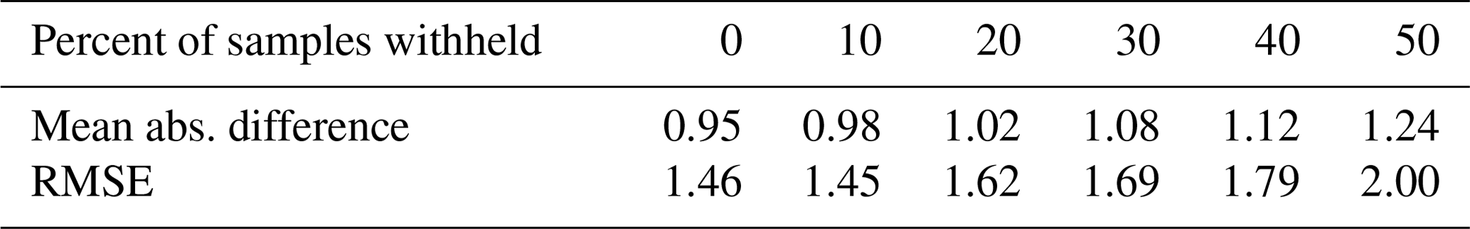
Table A2 Effect of altering random seed number on error obtained using the test dataset and the SO₂ height retrieval result after application to OMI. For the results, heights for two different pixels within the orbit from the Raikoke event (24 June 2019) are shown. Heights were retrieved using separate inverse models trained using 10 random states.

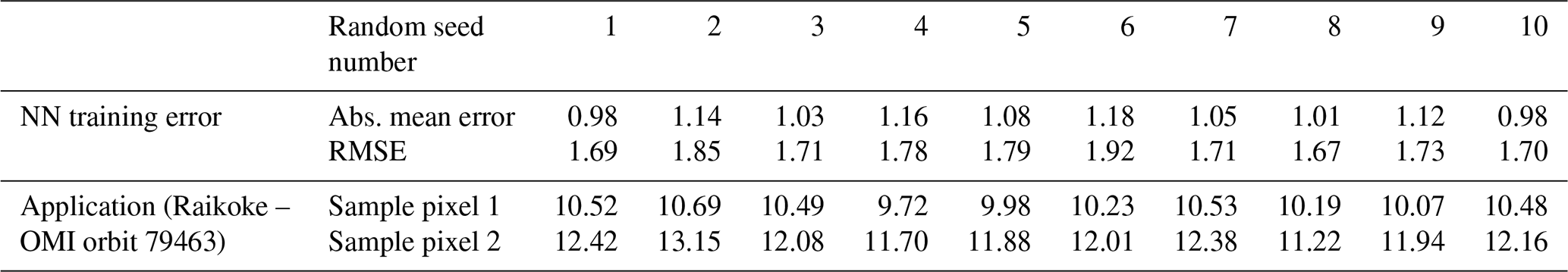
Figure A1 SO₂ VCD for the four volcanic cases: (a) Kasatochi on 10 August 2008, (b) Kelud on 14 February 2014, (c) Calbuco on 24 April 2015, and (d) Raikoke on 24 June 2019. In these maps, only pixels with SO₂ > 10 DU are shown.