the Creative Commons Attribution 4.0 License.
the Creative Commons Attribution 4.0 License.
 | 18 Jan 2021
Simulated reflectance above snow constrained by airborne measurements of solar radiation: implications for the snow grain morphology in the Arctic
Soheila Jafariserajehlou
Vladimir V. Rozanov
Marco Vountas
Charles K. Gatebe
John P. Burrows
Accurate knowledge of the reflectance from snow/ice-covered surfaces is of fundamental importance for the retrieval of snow parameters and atmospheric constituents from space-based and airborne observations.
In this paper, we simulate the reflectance in a snow–atmosphere system, using the phenomenological radiative transfer model SCIATRAN, and compare the results with that of airborne measurements. To minimize the differences between measurements and simulation, we determine and employ the key atmospheric and surface parameters, such as snow grain morphologies (or habits).
First, we report on a sensitivity study. This addresses the requirement for adequate a priori knowledge about snow models and ancillary information about the atmosphere. For this aim, we use the well-validated phenomenological radiative transfer model, SCIATRAN. Second, we present and apply a two-stage snow grain morphology (i.e., size and shape of ice crystals in the snow) retrieval algorithm. We then describe the use of this new retrieval for estimating the most representative snow model, using different types of snow morphologies, for the airborne observation conditions performed by NASA's Cloud Absorption Radiometer (CAR).
Third, we present a comprehensive comparison of the simulated reflectance (using retrieved snow grain size and shape and independent atmospheric data) with that from airborne CAR measurements in the visible (0.670 µm) and near infrared (NIR; 0.870 and 1.6 µm) wavelength range. The results of this comparison are used to assess the quality and accuracy of the radiative transfer model in the simulation of the reflectance in a coupled snow–atmosphere system.
Assuming that the snow layer consists of ice crystals with aggregates of eight column ice habit and having an effective radius of ∼99 µm, we find that, for a surface covered by old snow, the Pearson correlation coefficient, R, between measurements and simulations is 0.98 (R2∼0.96). For freshly fallen snow, assuming that the snow layer consists of the aggregate of five plates ice habit with an effective radius of ∼83 µm and having surface inhomogeneity, the correlation is ∼0.97 (R2∼0.94) in the infrared and 0.88 (R2∼0.77) in the visible wavelengths. The largest differences between simulated and measured values are observed in the glint area (i.e., in the angular regions of specular and near-specular reflection), with relative azimuth angles ∘ in the forward-scattering direction. The absolute difference between the modeled results and measurements in off-glint regions, with a viewing zenith angle of less than 50∘, is generally small and does not exceed ±0.05. These results will help to improve the calculation of snow surface reflectance and relevant assumptions in the snow–atmosphere system algorithms (e.g., aerosol optical thickness retrieval algorithms in the polar regions).
- Article
(21472 KB) - Full-text XML
- BibTeX
- EndNote


The extent and type of snow and ice cover have a significant impact on climate, as noted by Arrhenius over 100 years ago (Arrhenius, 1896). There is a positive feedback between decreasing surface temperature, an increase in snow and ice cover, and an associated increase in planetary albedo, which then further decreases surface temperature and vice versa. Consequently, changes in snow and ice extent and morphology play a key role in climate change. Having accurate knowledge about snow/ice-covered surfaces is a prerequisite for identifying and quantifying changes in the climate (Schneider and Dickinson, 1974; Curry et al., 1995; Cohen et al., 2014; Kim et al., 2017; Wendisch et al., 2017, 2019).
In addition, during recent decades, the Arctic region has warmed more rapidly than other regions. This phenomenon is known as the Arctic amplification (AA; Serreze and Barry, 2011). The analysis of the growing number of long-term records of the data products (e.g., the amount of trace gases, aerosol, and cloud parameters) retrieved from passive and active satellite observations provides potentially invaluable information for identifying and quantifying the evolution and consequences of AA (Wendisch et al., 2017).
Because of the magnitude of the scattering from snow, the use of remote sensing measurements above snow-covered surfaces in the cryosphere requires accurate models of the scattering and reflectance from snow surfaces. However, the current differences between simulated and measured reflectance in a coupled snow–atmosphere system lead to systematic errors in the determination of the atmospheric constituents, in particular for clouds and aerosol parameters but also trace gases (e.g., Istomina et al., 2010; Istomina, 2012; Jafariserajehlou et al., 2019).
A large number of experimental and theoretical studies have been conducted measuring and modeling snow optical properties, such as the angular distribution of reflected light over and within the snow surface and the subsequent derivation of snow albedo. The early measurements by Middleton and Mungal (1952) and the model of Dunkle and Bevans (1956) used to analyze the transmittance and reflectance of snow cover were the beginning of considerable efforts on this topic. Barkstrom (1972) formulated and solved the scattering problem for snow surfaces in terms of the radiative transfer theory. Later, the comparison of reflectance from snow-covered surfaces simulated by radiative transfer models (RTMs) with that of observation made substantial progress in our understanding of the angular distribution of reflectance above snow surface (e.g., Wiscombe and Warren 1980; Warren et al., 1998; Arnold et al., 2002; Painter et al., 2003; Kokhanovsky and Zege, 2004; Li and Zhou, 2004; Hudson et al., 2006; Hudson and Warren, 2007; Lyapustin et al., 2010; Kokhanovsky and Breon, 2012).
The reflection/scattering patterns of snow-covered surfaces can be summarized as follows: (i) snow is not a Lambertian reflector in the visible and near infrared spectral region because its reflectance has an anisotropic nature, and the anisotropy increases with wavelength; (ii) unlike other surface types (e.g., vegetation or soil) with a strong peak in back-scattering direction (the hot spot effect), snow has a strong forward peak for large viewing zenith angles (e.g., Gatebe and King, 2016); (iii) the snow reflectance variation is larger in the principal plane (i.e., the plane containing the Sun, surface normal, and observation direction) than in the cross plane (i.e., the one perpendicular to principal plane; Warren, 1982; Lyapustin et al., 2010; Kokhanovsky and Breon, 2012). However, the remaining discrepancies between simulated reflectance in a snow–atmosphere system and field measurements led to further investigations in the field of the single scattering properties of snow grains (Mishchenko et al., 1999; Jin et al., 2008; Yang and Liou, 1998; Yang et al., 2003, 2013), surface roughness (Warren et al., 1998; Hudson et al., 2006; Hudson and Warren, 2007; Lyapustin et al., 2010; Zhuravleva and Kokhanovsky, 2011), and atmospheric-correction methods (Lyapustin et al., 2010). Despite substantial improvements, the uncertainties in our understanding of the microphysical and macroscopic properties of snow are an unresolved issue for RTMs, ray tracing, and climate models. For example, the current state-of-the-art RTMs yield much more anisotropic reflectance behavior for snow in the glint region than observed in reality (Zhuravleva and Kokhanovsky, 2011; Lyapustin et al., 2010; Hudson and Warren, 2007; Warren et al., 1998). These studies either focus on the snow reflectance at the surface, employing an atmospheric-correction method (Leroux et al., 1998; Kokhanovsky and Zege, 2004; Kokhanovsky et al., 2005; Lyapustin et al., 2010; Negi and Kokhanovsky, 2011), or consider the atmospheric effects without in-depth investigations of the surface parameters (Aoki et al., 1999; Hudson et al., 2006; Kokhanovsky and Breon, 2012). A comprehensive study and investigation of both the snow layer and atmosphere parameters in a coupled snow–atmosphere system has not yet been undertaken but is required to improve the accuracy of remote sensing retrieval algorithms for aerosol and cloud in the Arctic region (Istomina et al., 2010; Istomina, 2012; Jafariserajehlou et al., 2019).
The intent of this paper is to (i) study the sensitivity of scattering and reflectance in the coupled snow–atmosphere system to both surface and atmospheric parameters, (ii) retrieve the most representative ice crystal morphology by applying a snow grain size and shape retrieval algorithm to measured reflectance, and (iii) evaluate the ability of a phenomenological RTM to reproduce the measured reflectance over the spectral range 0.34–1.649 µm at all available observation directions using the retrieved atmospheric and snow parameters.
In this study, we use the RTM SCIATRAN (Rozanov et al., 2014), which is a well-validated phenomenological RTM, and the airborne observations of reflectance acquired by the Cloud Absorption Radiometer (CAR). The CAR measurements were made during the Arctic Research of the Composition of the Troposphere from Aircraft and Satellite (ARCTAS) spring 2008 campaign over Barrow/Utqiaġvik, Alaska. Further information about the atmospheric parameters during the ARCTAS campaign was taken from available Aerosol Robotic Network (AERONET) and satellite data.
The paper is organized as follows: in the next section, we present the theoretical background and terminology used to calculate the angular distribution of reflectance in a snow–atmosphere system. In Sects. 3 and 4, we introduce and explain the measurements and the simulation methods. In Sect. 5, the sensitivity of reflectance to the underlying snow layer and atmospheric parameters is investigated. In Sect. 6, the results of applying the two-stage snow grain size and shape retrieval algorithm are presented. In Sect. 7, the results of the reflectance simulations are compared to CAR measurements. Finally, conclusions are drawn in Sect. 8. Appendix A contains a detailed description of the snow grain size and shape retrieval algorithm used in the study.
To describe the directional signature of reflectance over different surface types, the bidirectional reflectance distribution function (BRDF), as defined by Nicodemus (1965), is the commonly used reflectance quantity. The term BRDF describes the reflection of incident solar radiation from one direction to another direction (Nicodemus, 1965). The mathematical form of BRDF is expressed as follows (Nicodemus et al., 1977; Schaepman-Strub et al., 2006):
where Lr is the reflected radiance, and θ and φ are the zenith and azimuth angles, respectively. The subscripts of i and r correspond to the incident and to the reflected beams, respectively. E is the incident surface flux (irradiance), and λ is the wavelength. However, the BRDF is not a directly measurable quantity because of its formulation as a ratio of infinitesimal quantities (Nicodemus et al., 1977; Schaepman-Strub et al., 2006). Nicodemus et al. (1977) provided an extensive description of reflectance terminologies and measurable quantities, e.g., the bidirectional reflectance factor (BRF), the hemispherical directional reflectance factor (HDRF), the directional hemispherical reflectance (DHR), etc. According to Nicodemus et al. (1977) and Schaepman-Strub et al. (2006), each of the terms is defined for the specific illumination and reflectance geometries for which the reflectance properties are measured (e.g., satellite, airborne, or laboratory measurement conditions). Following the method of Gatebe and King (2016), the effective BRDF at a horizontal (flat) reference plane is defined as follows:
where is as an average of the BRDF over an appropriate area, angle, and solid angle for specific observation geometry. Δωi is a finite solid angle element. The validity of this approximation relies on the experimental evidence that the BRDF is not significantly influenced by the following effects: the finite intervals of area, angle, solid angle, and the distribution function, subsurface scattering, and radiation parameters such as wavelength, polarization, and fluorescence (i.e., significant variations do not occur within small intervals; see Nicodemus et al., 1977; Gatebe and King, 2016). As a result, the is determined by the following:
where is the measured radiance, and F0,λ is the solar irradiance incident at the top of atmosphere (TOA). Often, it is helpful to have a description of the difference between the measured surface reflectance and a Lambertian reflector; in such a case, it is the equivalent bidirectional reflectance factor , for which multiplied by π is more representative.
To isolate the reflectance properties of the surface and derive or just above the surface, we need to apply atmospheric-correction methods on the measured radiance at TOA or flight altitude (e.g., by using knowledge of the atmospheric scattering or absorption by applying RTMs). This removes the following four atmospheric contributions from the measured radiance at TOA or flight altitude (Schaepman-Strub et al., 2006): the contribution of light scattered by the atmosphere (i) before the solar radiation has reached the surface, (ii) after being reflected by the surface, (iii) before and after reaching the surface, and (iv) the atmospheric path radiance.
However, most of the atmospheric contributions in measurements close to the surface are negligible (except diffuse component number ii), and measured quantities represent the at-surface radiance (Schaepman-Strub et al., 2006). Sensitivity studies have demonstrated that atmospheric contributions to the CAR channel observations range from 3 % to 12 %, depending on the wavelength, in the range of 0.381 to 2.324 µm (Soulen et al., 2000). Consequently, previous studies presented either the BRFs in a surface–atmosphere system at flight altitude without atmospheric correction (Soulen et al., 2000) or the BRFs right above the surface after atmospheric correction (Gatebe et al., 2005; Gatebe and King, 2016).
The atmospheric-correction method relies on different assumptions by which several sources of uncertainty should be taken into account. In this study, to avoid such uncertainties, we do not apply an atmospheric correction to the measurements (radiances Lr, h) at flight altitude (h). Instead, we calculate and use the reflectance at flight altitude with the following equation:
where Lr, h is the measured radiance at flight altitude. All reflectance/ values at flight altitude in this study represent R in Eq. (4) and are referred to as the reflectance factor in the snow–atmosphere system.
In the simulation of the reflectance factor in a coupled snow–atmosphere system, we need to account for the atmospheric effects contribution properly. For this reason, we take independent data about atmospheric parameters (aerosol optical thickness, AOT, and gases absorption) from ground-based and space-borne measurements. We select the data with the closest spatial and temporal interval actual airborne measurements. We discuss more details of the atmospheric data and their application to the simulation routine in Sects. 3 and 4. To estimate just above the surface, further atmospheric correction is needed. We assume the reflectance factor at flight altitude is a good estimation of just above the surface at infrared wavelengths where atmospheric scattering is negligible.
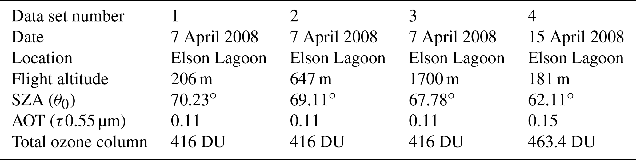
CAR is an airborne instrument developed at NASA's Goddard Space Flight Center. It has been used during several field campaigns around the world from 1984 up to the present. CAR has been used to measure the single scattering albedo of clouds, the bidirectional reflectance of various surface types, and for acquiring imagery of clouds and the Earth's surface. For this study, we used CAR data from the ARCTAS campaign conducted at Elson Lagoon, near Barrow/Utqiaġvik, Alaska, in April 2008 as part of the International Polar Year (Lyapustin et al., 2010; Gatebe and King, 2016). The goal of ARCTAS was to study physical and chemical processes in the Arctic atmosphere and (e.g., long-range transport of pollution to the Arctic) and surface parameters (e.g., snow reflectance angular variation). A P-3B aircraft carried the CAR instrument and was deployed by NASA from Fairbanks, Alaska. Figure 1 shows the flight track on 7 April 2008. The date, location, measurement geometry, and available atmospheric parameters during the measurements used in this study are presented in Table 1.

Figure 1Flight track of P-3B airplane carrying NASA's Cloud Absorption Radiometer (CAR) on 7 April 2008 during the Arctic Research of the Composition of the Troposphere from Aircraft and Satellite (ARCTAS) campaign (figure adapted from: https://www-air.larc.nasa.gov/missions/arctas/arctas.html, last access: November 2020). Image credits: © NASA; © Tele Atlas 2008; © Europa Technologies 2008; © TerraMetrics 2008; © 2007 Google.
Table 1Summary of the CAR, Aerosol Robotic Network (AERONET) aerosol optical thickness (transferred from 0.5 to 0.55 µm), and weighting function differential optical absorption spectroscopy (WFDOAS) ozone data used in this study. Note: solar zenith angle – SZA.
The unique design of CAR simultaneously provides both up-welling and down-welling radiances at 14 spectral bands (Table 2) located in the atmospheric window regions of UV, visible, and near-infrared from 0.34 to 2.3 µm, comprising important wavelengths relevant for remote sensing applications such as aerosol retrievals. Through a rotating scan mirror, the instrument provides viewing geometries suitable for measurements needed for BRF calculation. CAR collects the data with a mirror rotating 360∘ in a plane perpendicular to the direction of flight through a 190∘ aperture that allows the acquisition of data from local zenith to nadir or horizon to horizon with an angular resolution of 1∘. The high angular/spatial resolution of 1∘ in both the viewing zenith and azimuth angles allows the estimation of the anisotropy of the reflectance in the snow–atmosphere system with high accuracy.

The spatial resolution of CAR depends on the flight altitude, e.g., 10 and 18 m2 at nadir for 600 and 1000 m flight altitude, respectively, which increases with the viewing zenith angle (VZA), e.g., 580 m2 at 80∘ VZA for 1000 m flight altitude. The capability of acquiring data at different altitudes (∼200, 600, and 1700 m) enables us to evaluate the sensitivity of reflectance with respect to atmospheric effects in RTM simulations.
Examples of calculated reflectance factor values using Eq. (4) from CAR measurements on 7 April 2008 at Elson Lagoon (71.3∘ N, 156.4∘ W) are shown in Figs. 2 and 3. As we can see in these two figures, in spite of the influence of the atmospheric scattering and absorption, the general features of the snow BRF are clearly observable in polar plots and principal and cross-plane plots because of (i) the decrease in snow reflectance with increasing wavelength due to the increasing absorption by snow at longer wavelengths, (ii) the increase in the snow BRF as a function of VZA and the strong forward-scattering peak in the principal plane at large VZA, and (iii) the smaller angular variation in the BRF at cross plane compared to the principal plane, though the reflectance values increase with VZA. The snow surface spatial inhomogeneity decreases with increasing altitude due to the change in spatial resolution with altitude (Gatebe and King, 2016; Lyapustin et al., 2010). Accordingly, at poorer spatial resolutions, spatial homogeneity is more efficiently averaged, as can be seen in Fig. 2 at flight altitude of 1700 m, compared to 206 m, in which we have a higher spatial resolution.
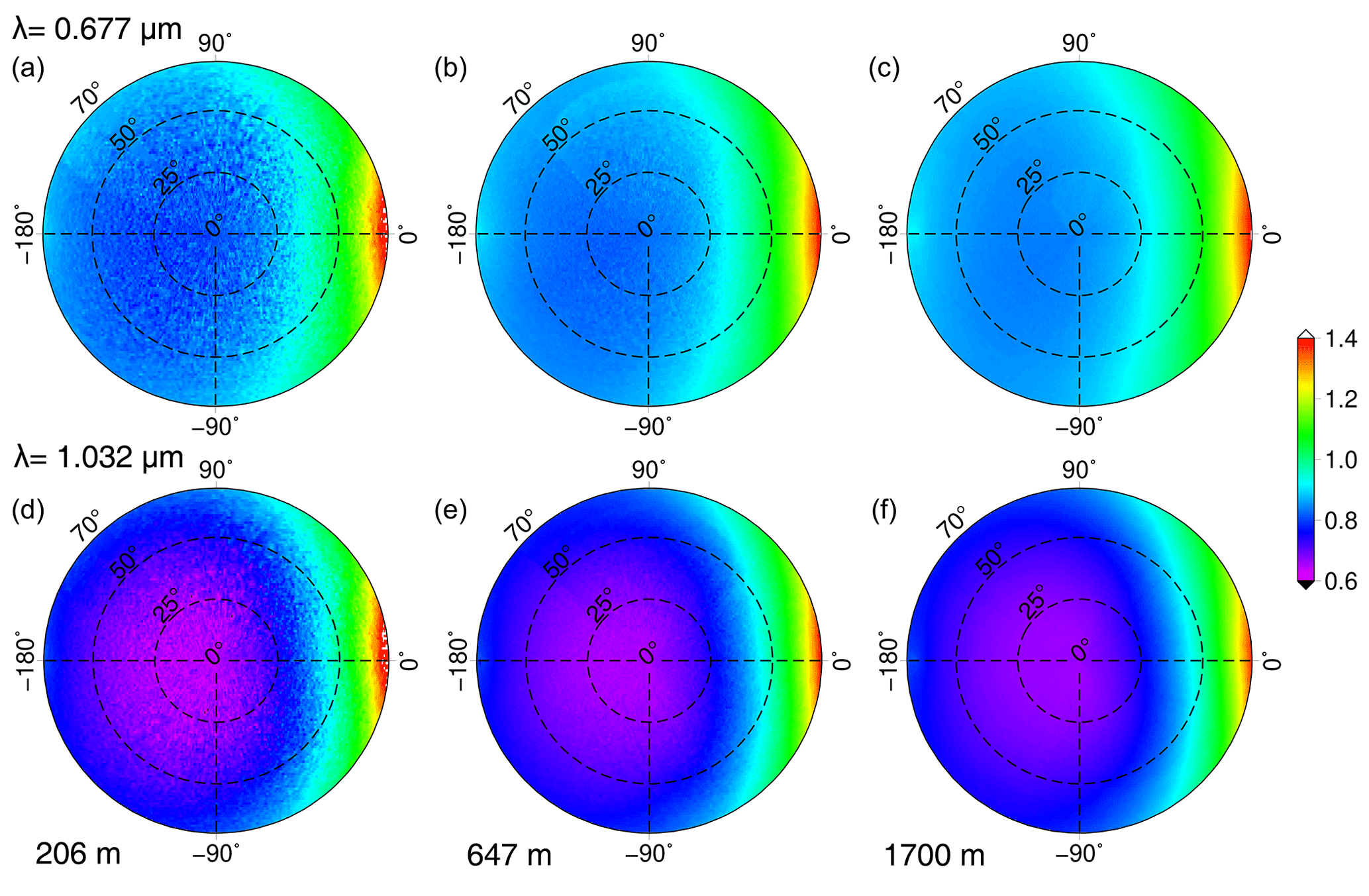
Figure 2Angular distribution of reflectance factor in the snow–atmosphere system derived from CAR measurements on 7 April 2008 at Elson Lagoon (71.3∘ N, 156.4∘ W), showing reflectance at the 0.677 µm wavelength and three flight altitudes of 206, 647, and 1700 m, respectively (a, b, c), and the 1.032 µm wavelength and the same flight altitudes (d, e, f). The principal plane is the horizontal line (φ=0 and 180∘), and the viewing zenith angle is shown as the radius of the polar plots from 0∘ (nadir) to 70∘. The solar zenith angle is 70.23, 69.11, and 67.78∘ for flight altitudes of 206, 647, and 1700 m, respectively.
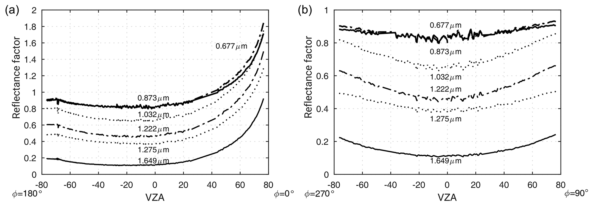
Figure 3Angular distribution of the reflectance factor in the snow–atmosphere system, derived from measurements by CAR at 647 m flight altitude and six wavelengths of 0.677, 0.873, 1.032, 1.222, 1.275, and 1.649 µm on 7 April 2008 at Elson Lagoon (71.3∘ N, 156.4∘ W). (a) The principal plane (φ=0 and 180∘) and (b) cross plane (φ=90 and 270∘).
To account for aerosols, we use the aerosol optical thickness (AOT) data acquired by the nearby Aerosol Robotic Network (AERONET) sun photometer at Barrow/Utqiaġvik during the CAR measurement time. AERONET is a globally distributed network and provides long-term and continuous ground-based measurements of the total column aerosol optical thickness derived from the attenuation of sunlight. The data are provided often at a high temporal resolution of 15 min. AERONET AOT data are provided at 0.5 and 0.6 µm wavelengths. We use the Ångström exponent to calculate AOT values at the reference wavelength (0.55 µm) required for the SCIATRAN simulation. Table 1 shows the calculated AOT at 0.55 µm, based on AERONET data for Barrow/Utqiaġvik at the closest time to the CAR airborne measurements. The aerosol condition and its chemical and optical properties have been measured continuously at Barrow, Alaska, during different seasonal periods (Quinn et al., 2002). Previous studies indicate the largest contribution from sea salt, non-sea-salt sulfate, and mineral dust. The average contribution of black carbon is very small compared to other aerosol types (Udisti et al., 2020). During the haze season (January to April), sea salt plays the dominant role in controlling light scattering in wintertime and non-sea salt sulfate in spring (Quinn et al., 2002). The increase in non-sea-salt (nss) sulfate in January to May is the long-range transport of anthropogenic primary nss sulfate, besides the long-range transport of anthropogenic SO2 and its photo-oxidization to nss sulfate with the increase of light levels, and the local production of biogenic nss sulfate.
To account for ozone absorption, we use knowledge of the ozone total column amount retrieved from the space-borne measurements by using the University of Bremen weighting function differential optical absorption spectroscopy (WFDOAS) algorithm version 4 (Weber et al., 2018). This data set (covering 1995 to the present) consists of merged total ozone column data retrieved by WFDOAS from the Global Ozone Monitoring Experiment (GOME), Scanning Imaging Absorption Spectrometer for Atmospheric Chartography (SCIAMACHY), and GOME-2A. In this paper, the ozone total column data are selected using the criteria of having the smallest temporal and spatial differences with CAR data. For nitrogen dioxide, we use vertical column information from the SCIATRAN database obtained from a 2D chemical transport model developed at the University of Bremen (Sinnhuber et al., 2009).
The derived AOT and trace vertical column have been used in the simulation of radiative transfer processes in the snow–atmosphere system.
SCIATRAN is a software package for radiative transfer modeling developed at the Institute of Environmental Physics (IUP), University of Bremen (Rozanov et al., 2002, 2014), and freely available at http://www.iup.uni-bremen.de/sciatran/ (last access: February 2020). The SCIATRAN package has been used in a variety of remote sensing studies to simulate radiative transfer processes in a wide spectral range, from the ultraviolet to the thermal infrared (0.18–40 µm), assuming either a plane parallel or a spherical atmosphere (Rozanov et al., 2014).
In this paper, to calculate the reflectance factor values, SCIATRAN assumes that the snow is a layer with an optical thickness of 1000 and a geometrical thickness of 1 m, composed of ice crystals of different morphologies and placed above a black surface. This assumption was successfully validated by Rozanov et al. (2014). The snow layer is assumed to be vertically and horizontally homogeneous and composed of a monodisperse population of ice crystals. The impact of impurities in the snow (e.g., black carbon) is neglected in this study. To simulate the radiative transfer through a snow layer, the single scattering properties of ice crystals, including extinction and scattering efficiencies, single scattering albedo, and phase functions, need to be defined in SCIATRAN. All these parameters are dependent on the wavelength, size, and shape of the particle (Leroux et al., 1999). Recently, a new data library of basic single scattering properties of nine ice crystal shapes/habits developed by Yang et al. (2013) has been incorporated in the SCIATRAN model (Pohl et al., 2020). This database comprises a full set of single scattering properties at wavelengths from the UV to the far infrared (IR) for the following nine ice crystal morphologies: droxtal, column and hollow column, aggregate of eight columns, plates, small aggregate of five plates, large aggregate of 10 plates, and hollow and solid bullet rosettes. More detailed information about the ice crystal shapes and sizes can be found in Yang et al. (2013). In addition to the abovementioned nine ice crystals, optical parameters for triadic Koch fractal (referred to as fractal in this paper) particles are used as well (Macke et al., 1996; Rozanov et al., 2014). The fractal particle model uses regular tetrahedrons as its basic elements. In this study, we use the second-generation fractals, as described in Macke et al. (1996) and Rozanov et al. (2014).
In SCIATRAN, the snow grains are specified by their single scattering properties of sparsely distributed particles. Namely, the snow grains are assumed to be in the far field zones of each other and will thus scatter the light independently. For a snow layer, the snow grains can be located in each other's near field, resulting in interactions between the scattered electromagnetic fields of neighboring particles which lead to the modification of single scattering properties (Mishchenko, 2014; Mishchenko, 1994). The impact of the near-field effect was investigated in Pohl et al. (2020), using the modified single scattering properties of sparsely distributed particles, as suggested in Mishchenko (1994). The comparison of snow BRFs calculated assuming sparsely or densely packed snow layers shows that the maximum difference does not exceed 0.015 % (Pohl et al., 2020). Therefore, this effect was ignored in radiative transfer calculations through the snow layer.
To account for atmospheric effects, SCIATRAN incorporates a comprehensive database containing monthly and zonal vertical distributions of trace gases, e.g., O3, NO2, SO2, H2O, etc., spectral characteristics of gaseous absorbers, vertical profiles of pressure and temperature, and molecular scattering characteristics (see Rozanov et al., 2014, for details). To account for scattering and absorption by aerosols over snow in SCIATRAN, the optical characteristics of aerosol particles and vertical distribution of aerosol number density are required. In this study, we use Moderate Resolution Imaging Spectrometer (MODIS) collection 5 aerosol parameterization (Levy et al., 2007) as an internal database in SCIATRAN. Levy et al. (2007) developed a framework for connecting the aerosol microphysical properties, such as the refractive index and size distribution to the AOT at 0.55 µm. Using AOT from ground-based measurements of AERONET at Barrow/Utqiaġvik, as mentioned, and selecting one of the aerosol types, the Mie code incorporated into SCIATRAN is employed to calculate aerosol extinction and scattering coefficients. In this study, the vertical profile of aerosol number density, as an exponential vertical distribution for a height of 3.0 km, is used.
For the conditions described above, the radiative transfer calculations are performed at a source–target–sensor geometry extracted from the airborne measurements at solar zenith angles of 70.23, 69.11, 67.68, and 62.11∘ together with a viewing zenith angle (0–70∘) and relative azimuth angle (0–360∘), with an angular resolution of 5∘, and at four different altitudes of 181, 206, 647, and 1700 m. More detailed information about atmospheric and snow layer parameters are given and discussed separately in the following section.
The measured reflectance in the visible and near infrared (NIR) spectral range over a snow field depends on the relative importance of the absorption and scattering radiative transfer processes in the atmosphere and snow layer. In this section, we investigate the sensitivity of the reflectance on the radiative transfer through the atmosphere and the snow at the selected wavelength bands (i) 1.649 µm, because of the high sensitivity of this wavelength to snow grain properties, and (ii) 0.677 and 0.873 µm wavelengths, because of the relatively high and differing sensitivities at these wavelengths to the atmospheric conditions being used for aerosol optical thickness retrievals.
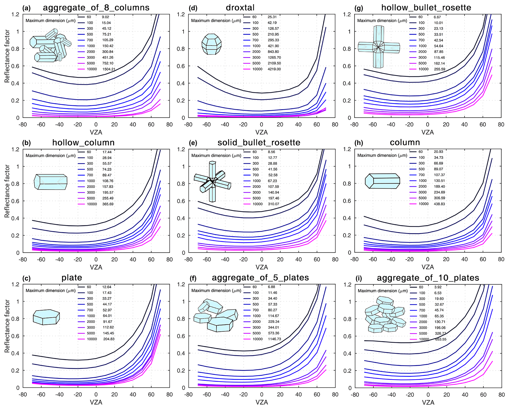
Figure 4The change in reflectance factor values in the principal plane (φ=0 and 180) with the size and shape of ice crystals at the wavelength of 1.649 µm. The left column of the legend in each panel shows the maximum length of the ice crystal, and the right column is its equivalent effective radius.
5.1 Impact of snow: size and shape of ice crystals
To study the influence of ice crystal morphology on the radiation field above snow-covered surfaces, we perform the simulation at 1.649 µm for the following three important reasons (Leroux et al., 1998):
- i.
The absorption of ice crystals is small or negligible at the selected wavelengths in the visible domain of the spectrum. In contrast, in the near-infrared range, due to the large absorption of ice crystals at these wavelengths, the snow reflectance is significantly affected by the snow grain size – the larger the particle, the smaller the reflectance because of larger absorption and stronger forward scattering.
- ii.
The BRF properties of snow at 1.649 µm are closer to those for single scattering behavior, and this is linked to the phase function, which strongly depends on the shape of ice crystals.
- iii.
The impact of the atmosphere (absorption by CO2 and H2O and diffuse incident irradiance) at 1.649 µm is negligible.
To illustrate the high sensitivity of the radiation field to the varying sizes of ice crystals at 1.649 µm, we simulated the snow reflectance factor at principal and cross planes, assuming nine ice crystal morphologies with varying sizes (here size refers to maximum dimension/edge length), 60∼10 000 µm, and three different roughnesses (smooth surface – 0; moderate surface roughness – 0.03; severe surface roughness – 0.50). For further information, see Yang et al. (2013). Figure 4 shows the simulated reflectance factor versus the VZA in the principal plane (as the most sensitive and representative direction for the largest changes of reflectance) using severely roughened morphology. As can be seen in Fig. 4, the reflectance factor strongly changes with the size of ice crystals from 60 to 10 000 µm. The equivalent effective radius1 is shown beside the maximum lengths of ice crystals in Fig. 4. Differentiating between various shapes has the largest effect in the forward-scattering (φ=0∘) and a lesser effect in backward-scattering direction (φ=180∘). The results indicate that the effect of changing size is larger than the impact of differentiating between various shapes of ice crystals at this wavelength.
Using the aggregate of eight columns shape and changing the maximum dimension from 60 to 10 000 µm results in a reflectance decrease of ∼40 % at the nadir (VZA∼0∘) and more than 80 % in the forward-scattering direction (at VZA of 60∘), which is considerably large. If we change only the shape of the snow grain from an aggregate of eight columns to the droxtal, but we keep the size (largest dimension) as it is (e.g., 300 µm), this change provides a noticeable decrease of ∼30 % in reflectance at the forward-scattering direction for a viewing zenith angle of 60∘, and this leads to a much weaker forward peak. What is noteworthy is that the plate shape cannot reproduce the enhancement in a backward direction (typical for a BRF over snow) that is as strong as what the aggregate of eight columns or the droxtal shape causes. Using the aggregate of five and 10 plates leads to larger reflectance in all directions compared to the single plate shape. However, the analysis of the simulation results at the cross plane (not shown here) indicates that the impact on the reflectance pattern, originating from the specific shapes of the ice crystals, is relatively small compared to the impacts at the principal plane.
The large range of changes in the reflectance in both the principal and cross planes, when using different ice crystal morphologies, highlights the importance of having accurate a priori knowledge or estimations of the size and shapes of the ice crystals to accurately reproduce measurements. In our study, due to the lack of such information from in situ measurements, we estimate the size of ice crystals for each selected crystal shape separately to have a priori knowledge of ice crystal properties and to limit the differences between the simulated and measured reflectance. The detailed explanation and results are given in Sect. 6.
5.2 Impact of atmosphere: scattering and absorption by aerosol and gases
The incident radiation is composed of direct sunlight and the diffuse radiation from the sky (Aoki et al., 1999). To take the atmospheric absorption and scattering into account, we assume an atmosphere over the snow layer, which contains (i) Rayleigh scattering (scattering by air molecules), (ii) gaseous absorption, and (iii) absorption and scattering by aerosols. Therefore, in this section, absorption bands, e.g., 0.677 µm are selected to evaluate the impact of the atmosphere. We calculate the reflectance factor at 0.677 µm under three different conditions, assuming a model atmosphere governed, (i) by Rayleigh scattering, (ii) identical to (i) but with absorption by ozone (O3) and nitrogen dioxide (NO2), and (iii) identical to (ii) but including aerosol. The calculations are performed assuming the following properties of the atmosphere and snow layer:
- i.
Vertical profile of nitrogen dioxide, pressure, and temperature are selected according to a 2D chemical transport model (Sinnhuber et al., 2009) incorporated in SCIATRAN.
- ii.
Total vertical column of ozone and AOT are set according to Table 1.
- iii.
Snow layer is composed of ice crystals having the shape aggregate of eight columns, a maximum dimension of 650 µm, and a severely roughened crystal surface.
Figure 5 shows the impact of the atmosphere and the difference between measured and simulated reflectance factor values at three different altitudes (206, 647, and 1700 m) for the three scenarios. The reflectance reduction at 647 m flight altitude due to gaseous absorption is the smallest (∼5 %) close to the nadir region and becomes larger (∼10 %) in the forward-scattering direction, which decreases (to ∼8 %) at 1700 m altitude. At this wavelength, ozone with a vertical optical depth (VOD) of has a much larger contribution to gaseous absorption compared to that of NO2 with a VOD of .

Figure 5Measured and simulated reflectance factor at 0.677 µm versus the viewing zenith angle (VZA) in the principal plane (φ=0 and 180∘) at three different flight altitudes. Panels represent results at 206, 647, and 1700 m flight altitudes, respectively. The green lines indicate simulated reflectance assuming Rayleigh scattering (case i). The blue line shows reflectance for case ii (as in case i, including absorption of O3 and NO2). The orange lines show the reflectance for case iii (as in case ii but adding aerosol with an aerosol optical thickness (AOT) of 0.11 for three types of aerosol, namely (i) weakly absorbing, (ii) moderately absorbing, and (iii) strongly absorbing).
The reflectance for an atmosphere containing three types of aerosol (weakly, moderately, or strongly absorbing aerosol) and without aerosol (containing only Rayleigh and gaseous absorption) is presented in Fig. 5. For more information on the aerosol typing used in this study see Levy et al. (2007). The changes in reflectance, due to weakly absorbing aerosol with an AOT of 0.11 (measured by AERONET) at 206 m flight altitude, are ∼5 % at the nadir and an increase in the forward-scattering direction to ∼13 %. The strongly absorbing aerosol (at the same AOT of 0.11) reduces the reflectance by ∼7 % at the nadir and ∼20 % in the forward-scattering direction. At 1700 m, the reflectance decreases by 6 % at the nadir and 7 % in the forward-scattering direction. The differences between the three aerosol types does not lead to changes in reflectance which are larger than 5 % in or close to nadir areas. In summary, an atmosphere containing Rayleigh scattering, absorption by ozone (O3) and nitrogen dioxide (NO2), and weakly absorbing aerosol is the best representation of the atmospheric conditions for our case study.
In the previous section, we showed that having adequate a priori information about the snow surface and atmosphere is necessary for calculating the reflectance factor with sufficient accuracy. In contrast to the atmospheric parameters available from independent sensors and models, a priori knowledge about ice crystal size and shape for the underlying snow layer is not typically available. To estimate the optimal ice crystal morphology, we used a snow grain size- and shape-retrieval algorithm by minimizing the difference between the measured and simulated reflectance factor (see Appendix A for details). Here, size refers to the effective radius of the ice crystal. The retrieval algorithm is applied to measurements at principal and cross planes at 1.649 µm, assuming different shape and crystal surface roughnesses. To find the best representative shape and size, the bias and root mean square error (RMSE) between the measured and simulated reflectance factor were determined for each case study.
Figure 6 shows one example of the comparison between the measured and simulated reflectance factor at principal and cross planes. The absolute uncertainty of CAR measurements is within 5 % and is shown by the uncertainty envelope (shading). The accuracy of our radiative transfer calculations is estimated to be in the range of 0.1 %. Based on the comparison, one can state that the angular reflectance pattern of the CAR measurement on 7 April 2008 at Elson Lagoon is reproduced by SCIATRAN successfully. The highest accuracy is obtained by assuming ice crystals as an aggregate of eight columns with severely roughened crystal surface at an effective radius of 98.8 µm (corresponding to a maximum dimension of 650 µm). In this case, the largest and smallest discrepancies appear in the forward-scattering direction and close to the nadir (∘), respectively. The overall RMSE and bias between measurements and simulation at the principal plane is 6.9 % and 2.7 %, respectively. A lesser degree of agreement between simulated results and measurements is provided by using column and fractal shapes with an RMSE of 7.3 % and 9.75 %, respectively. The largest difference between measurements and simulations is observed for the case using the droxtal shape with an RMSE ∼25.54 %.

Figure 6Comparison of measured and simulated reflectance factors. Measurements were performed by the CAR instrument over old snow at 647 m flight altitude on 7 April 2008 at 1.649 µm. The uncertainty in CAR measurements is indicated by the envelope (shading). SCIATRAN simulations in the principal and cross plane given by the dashed–dotted and dotted lines, respectively, and by different colors (green, blue, and red) present smooth, moderately roughened, and severely roughened crystal surfaces. Positive and negative VZAs correspond to azimuthal angles φ=0 and 180∘ for the principal plane and φ=90 and 270∘ for the perpendicular plane, respectively.
We also retrieved the effective radius of ice crystal using CAR data for fresh fallen snow on 15 April 2008. Due to the existing surface horizontal inhomogeneity for the case of fresh snow acquired at a lower flight altitude ∼181 m, larger differences between simulated and measured reflectance are expected, compared to the old snow case on 7 April 2008. The results are shown in Fig. 7. Unlike the old snow case presented in Fig. 6, the aggregate of eight columns shape does not optimally represent the ice crystals of this particular day. Rather, a reflectance simulated by using an aggregate of five plates as the ice crystal shape provides the minimum RMSE ∼12.85 % between the measurement and simulation results. An aggregate of 10 plates and fractal provide the second and third most representative shapes, with an RMSE of ∼13.16 % and 14.69 %, respectively. The results obtained by using the droxtal ice crystal shape exhibit large differences in both of forward- and backward-scattering directions with an RMSE of 34.1 %.
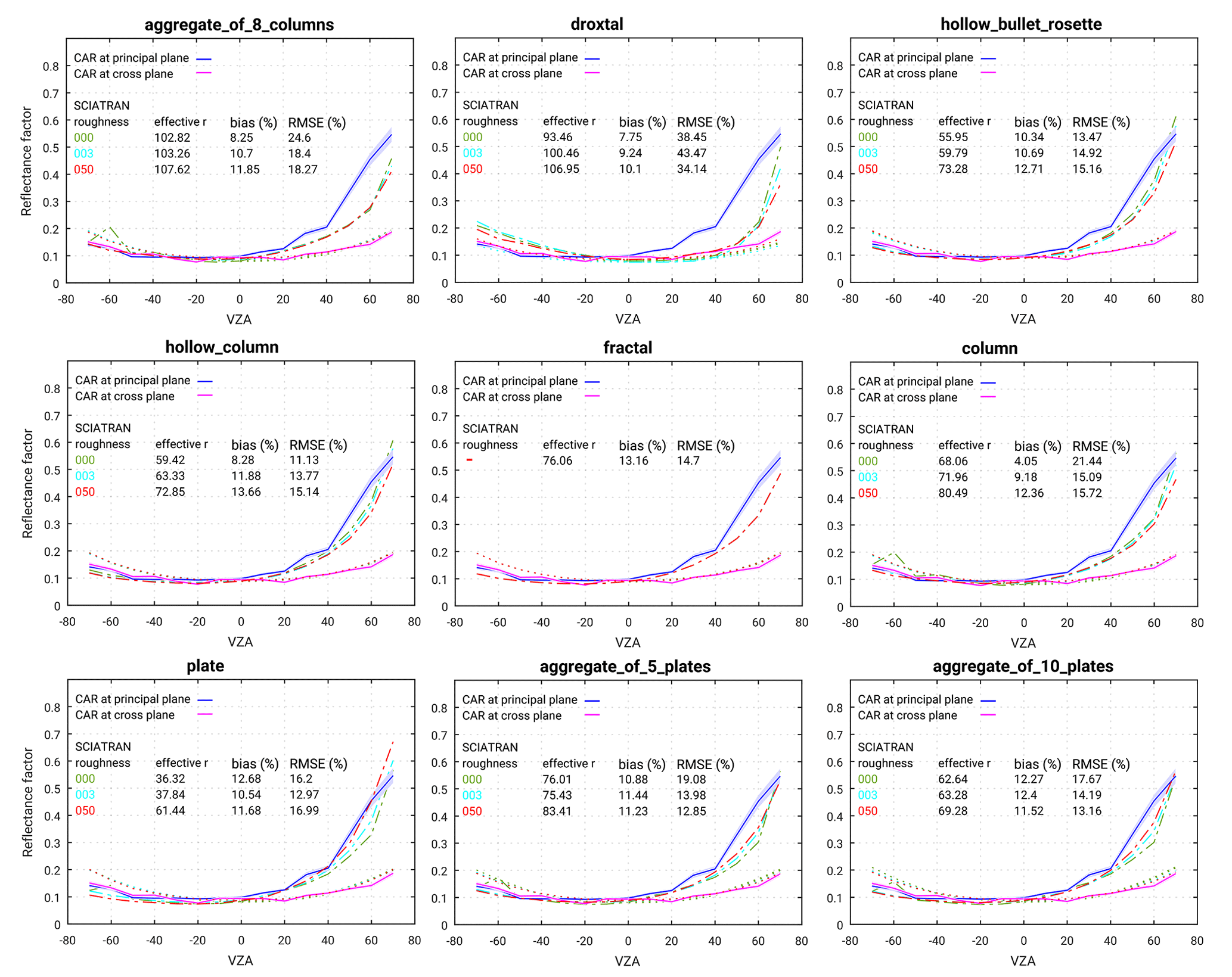
Figure 7The same as Fig. 6 but the measurements by the CAR instrument were performed on 15 April at 181 m flight altitude over fresh snow.
Though the real nature of the ice crystal shape at the time of measurement is not known to us, the impact of temperature and supersaturation on the morphology of snow grain particles has been debated in previous studies (Slater and Michaelides, 2019; Shultz, 2018; Libbrecht, 2007; Bailey and Hallett, 2004; Yang et al., 2003). Based on the relationship between temperature and snow grain morphology, the column-based shapes are the dominant ice crystal morphology in environments with temperatures higher than −10 ∘C, whereas plates are dominant if the temperature is less than −10 ∘C. Though more investigation is needed, especially to account for the temperature profile at the exact time of snowfall, our findings with respect to the most representative shape for each case study agree with this argument. The temperature range during CAR measurements on 6–7 April 2008 is from −20 to −5 ∘C. Based on our results, the aggregate of eight columns is the most representative shape for measurements conducted on this day. On 15 April 2008, when the temperature range changes to −23 to −17 ∘C, mainly plate-based ice crystal shapes are expected for such low temperatures, and our results confirm this argument. In addition, the existence of droxtal ice crystals during the measurement is less probable because very low temperatures ( ∘C) are needed to form droxtal or quasi-spherical ice crystals (Yang et al., 2003). The temperature dependence of the ice crystal morphologies explains, in part, why droxtal-shaped ice crystals do not capture the derived snow reflectance values from CAR measurements in any of our scenarios. With respect to the size of ice crystals, we do not compare fresh and old snow cases because it is important to note that the date of the old snow case is before fresh snow. This means the studied old snow case is not the aged fresh snow case. Therefore, the change in ice crystal size with its age is not studied in the scope of this paper.
Table 3Retrieval of the physical characteristics of ice crystals with different shapes in the case of most roughened habits. Numbers in italics indicate minimum root mean square error (RMSE).
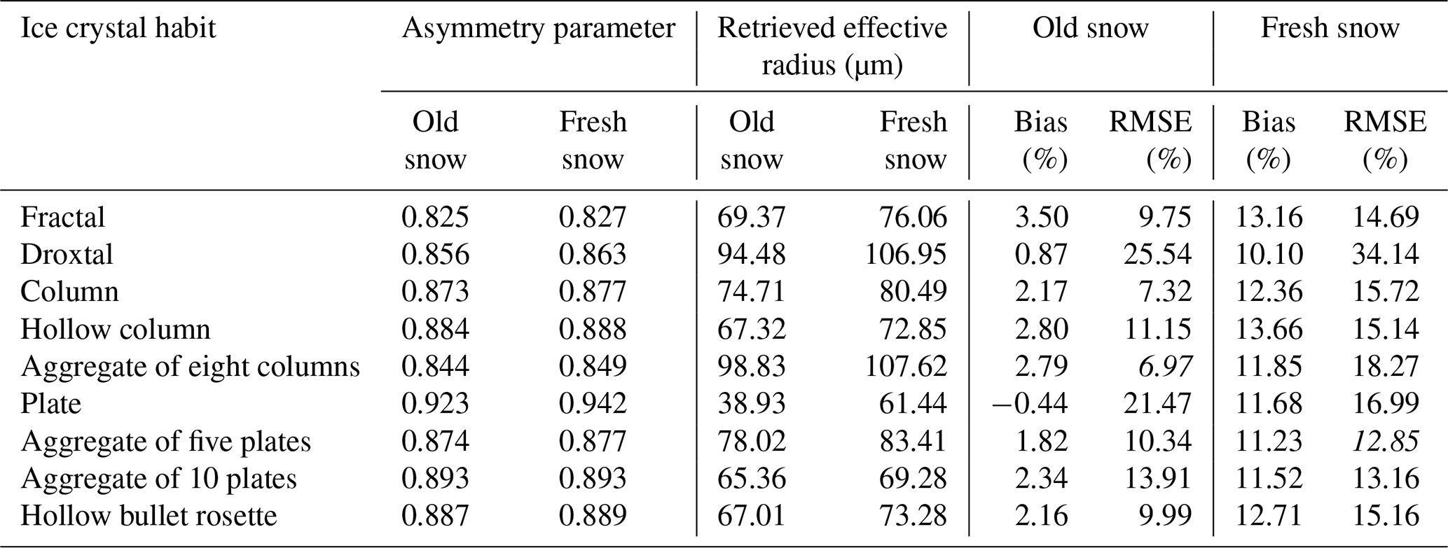
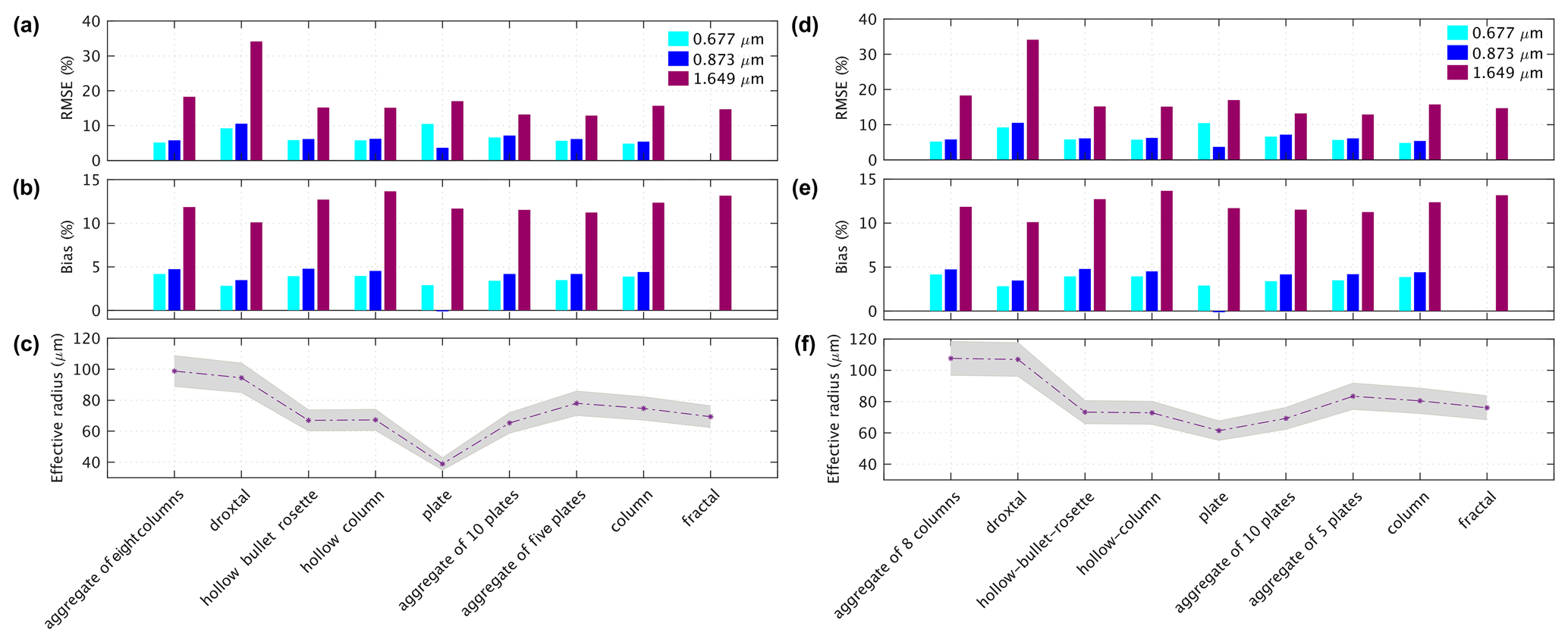
Figure 8Comparison of snow grain size retrieval and best fit of reflectance at three wavelengths of 0.677, 0.873, and 1.649 µm. (a, b, c) Old snow case and (d, e, f) fresh snow case. Effective radius is retrieved at 1.649 µm, and the gray envelope (shading) shows the uncertainty in the retrieved effective radius.
A summary of retrieved effective radii using different ice crystal shapes and corresponding bias and RMSE values is presented in Table 3. The ice crystals with a minimum RMSE value at 1.649 µm are italicized and selected to be used for subsequent calculations of the reflectance factor at 0.677 and 0.873 µm. In Fig. 8, the importance of the ice crystal shape selection for the snow grain size retrieval and the snow reflectance calculation is highlighted. The measurements were selected from the old snow and fresh snow cases. The effective radius is retrieved only at 1.649 µm, and then it is used to calculate the reflectance factor at 0.677 and 0.873 µm. The results are presented in Fig. 8, with the corresponding RMSE and bias values in the principal plane. The uncertainty of the effective radius retrieval is estimated to be ∼10 %, on the basis of the optimal estimation technique, and is shown by the gray envelope (shading) in Fig. 8. It can be seen that the retrieved effective radius value changes from shape to shape. The difference in retrieved effective radius generally does not exceed 40 %, but in the case of the plate ice crystals, the retrieved effective radius is ∼70 % smaller than the other shapes, e.g., the aggregate of eight columns. This is a significantly large difference. However, these results are presented for the principal plane in which the maximum differences between simulation and measurement are expected. Therefore, the overall bias and RMSE value on all azimuth directions is smaller than what is presented here. It can be seen that the RMSE values at 0.677 and 0.873 µm are significantly smaller than that at 1.649 µm. This is explained by the high reflectance values at these wavelengths, and therefore the larger denominator in RMSE formula, in which the difference of measured and simulated reflectance factor is divided by the measured reflectance.
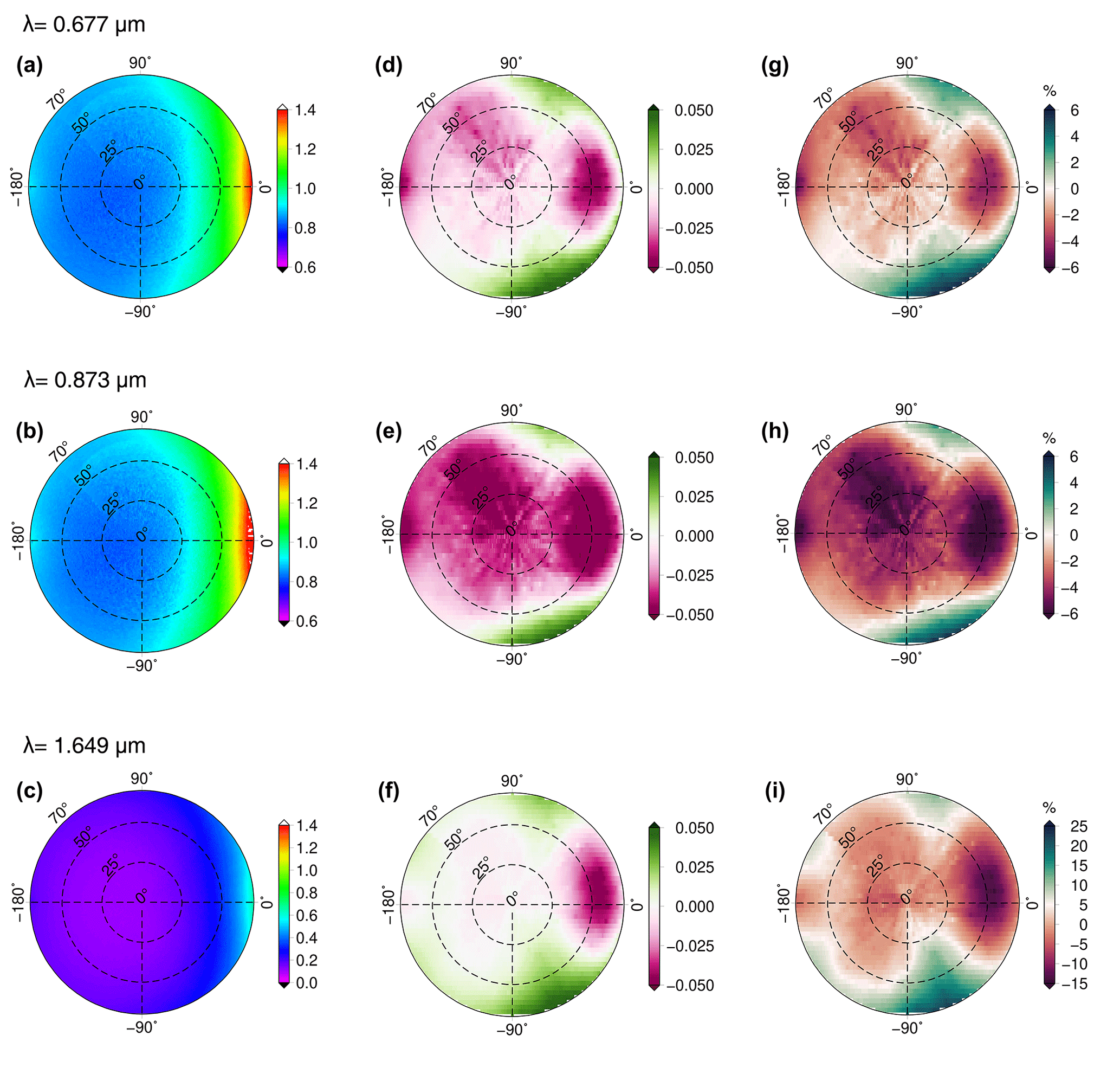
Figure 9(a, b, c) The reflectance factor at three wavelengths, namely 0.677, 0.873, and 1.649 µm, from the CAR measurements acquired on 7 April 2008 at Barrow/Utqiaġvik, Alaska, at an altitude of 647 m. (d, e, f) The absolute difference between reflectance of simulation (RSCIATRAN) and that of measurement (RCAR): (RSCIATRAN − RCAR). (g, h, i) The relative difference in percent (%).
In this section, we present the results of the comparison of the measured and simulated reflectance factor in the snow–atmosphere system. The simulations, which used the results and findings described in the previous section, were performed by assuming an atmosphere containing O3, NO2, and weakly absorbing aerosol, as described in Table 1. The snow layer is assumed to be comprised of an aggregate of eight column ice crystals, with a maximum dimension of 650 µm (effective radius 99 µm) for the case of the old snow, and an aggregate of five plates ice crystals, with a maximum dimension of 725 µm (effective radius 83 µm) for the case of the fresh snow.
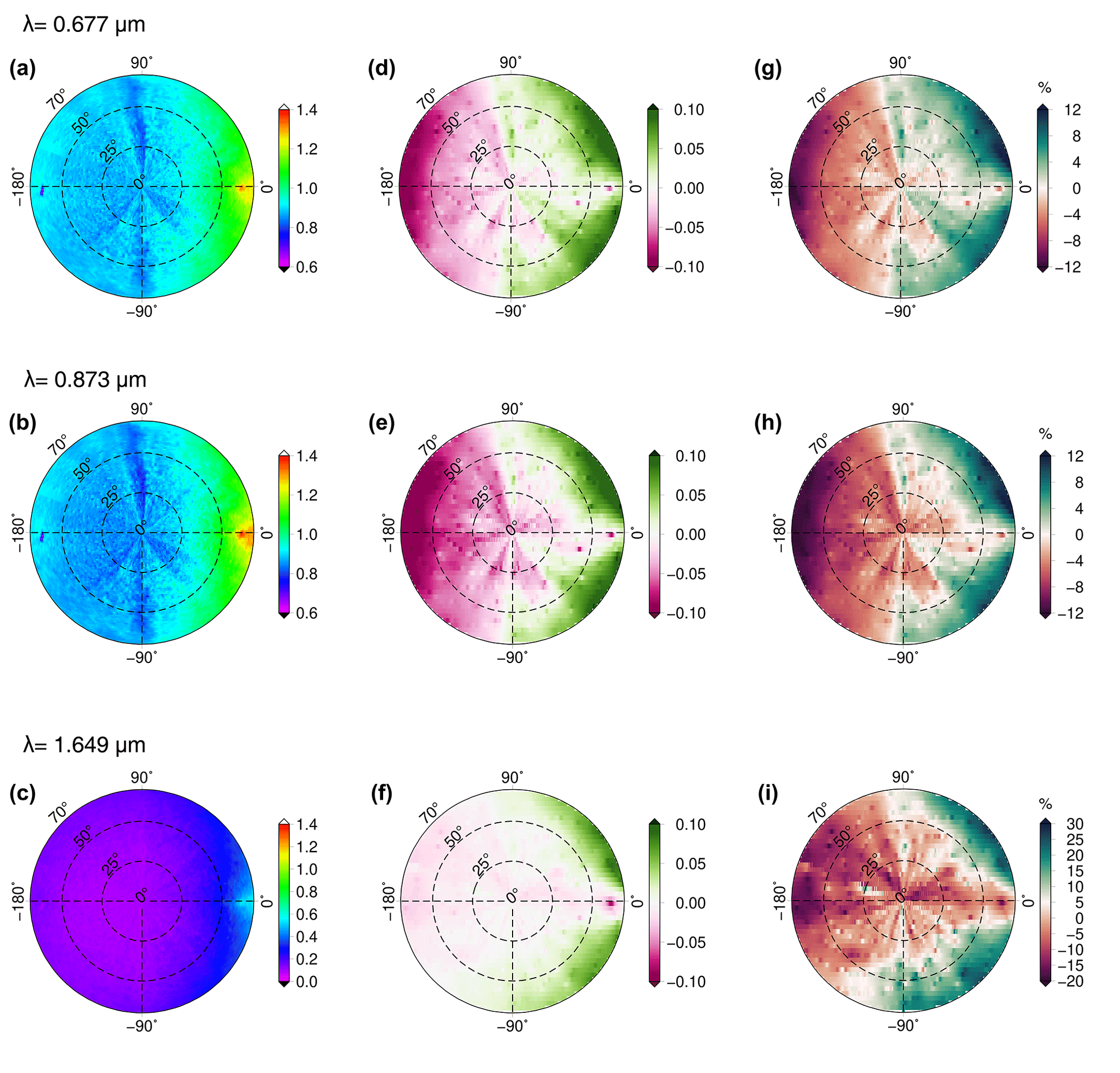
Figure 10The same as Fig. 9 but the measurements by the CAR instrument were performed on 15 April 2008 at 181 m flight altitude over fresh snow.
In Fig. 9, the difference between the simulated and measured reflectance factor at 0.677 and 1.649 µm is small on average, being less than 0.025 in regions of small VZA and not exceeding ±0.05 for larger VZA <50∘. These values are larger at 0.873 µm; the maximum difference reaches for small VZA. The difference between SCIATRAN simulation values and those of the measurements is pronounced in the forward-scattering region where |Δφ|<40∘. Figure 10 is the same plot as Fig. 9 but for fresh snow. The differences between the SCIATRAN simulations and CAR measurements of the reflectance factor are less pronounced in the glint region, compared to those for the old snow.
To assess the accuracy of the simulations over all azimuth angles, the correlation plot and the Pearson correlation coefficient between the measured and modeled reflectance factor are shown in Fig. 11. As it is shown in Fig. 11, the correlation coefficient between reflectance measurements over old snow and simulation is high, ∼0.98. We consider that surface inhomogeneities and related larger shadowing effects at a measurement altitude of 181 m explain why the correlation decreased to 0.88 at 0.677 µm (for the case of old snow, acquired at 647 m flight altitude, surface inhomogeneities are smoothed, and therefore, the old snow case is less affected by surface inhomogeneities). However, in Fig. 11, at 1.649 µm the correlation coefficient is high ∼0.97 for the case of fresh snow, possibly because of there being less sensitivity in this channel to shadowing and atmospheric scattering effects.
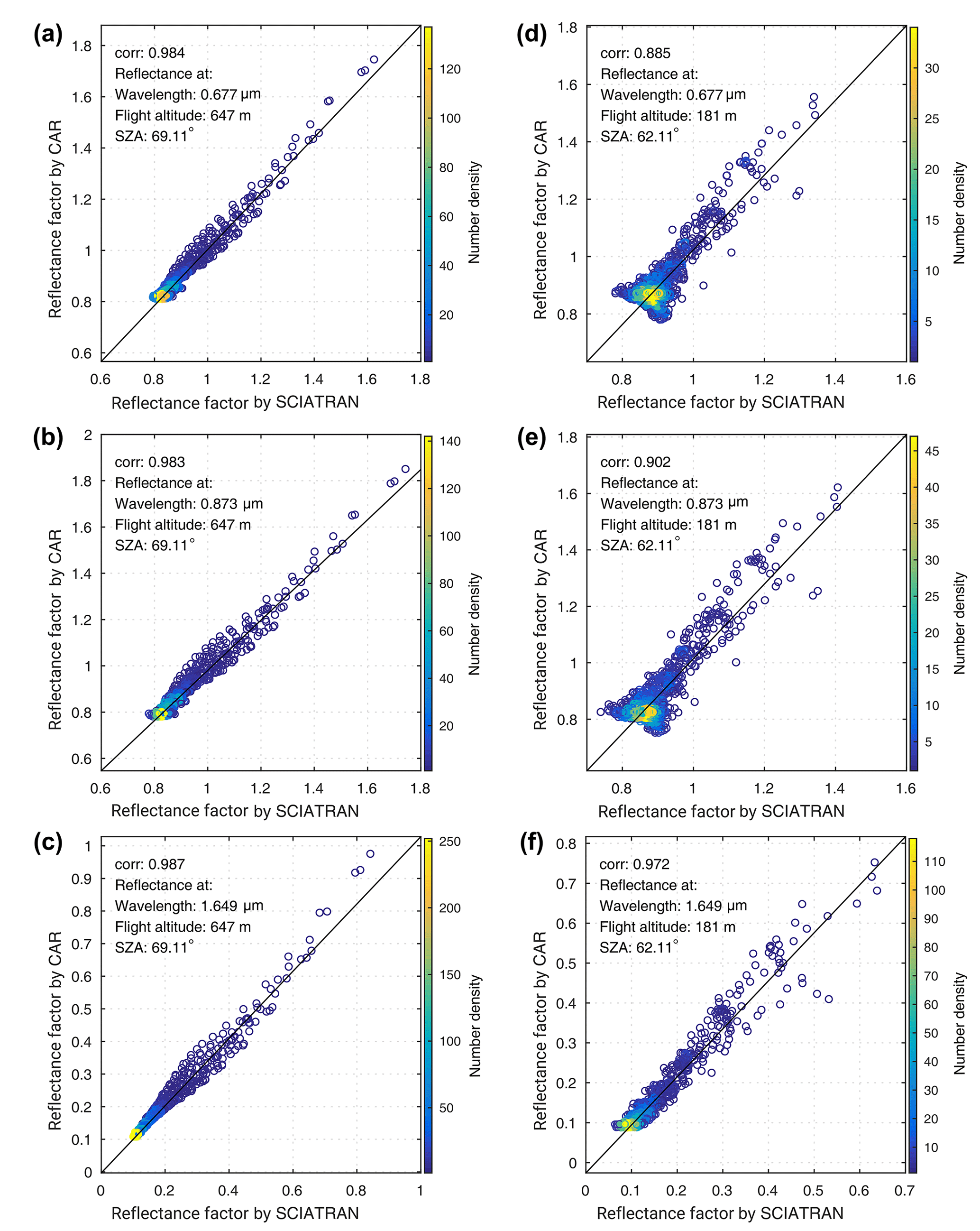
Figure 11The scatterplot with corresponding Pearson correlation coefficient of reflectance factor measured by CAR and simulated by SCIATRAN. (a, b, c) The results for old snow and (d, e, f) fresh snow. Here the color bar represents the number density of the pixels.
In this study, our objective was to assess the accuracy of the simulation of the reflectance in a snow–atmosphere system, taking different snow morphology and atmospheric absorption and scattering into account. For this, we used a state-of-the-art RTM, SCIATRAN, which used explicit models of the snow layer and the airborne CAR measurements.
The airborne CAR data were acquired by NASA over Elson Lagoon at Barrow/Utqiaġvik, Alaska, during the ARCTAS campaign in spring 2008. The spectral coverage of the airborne measurements is wide (0.3–2.30 µm), comprising important wavelengths relevant for remote sensing applications, such as aerosol retrievals, which could benefit from the results of this study. Measurements obtained at different flight altitudes (∼200, 600, and 1700 m) provide an opportunity to investigate the sensitivity of simulated reflectance to atmospheric parameters.
The SCIATRAN RTM (a phenomenological RTM) was used to simulate the reflectance factor in the snow–atmosphere system and its changes for different snow morphologies (i.e., snow grain size and shape). These simulations explicitly take atmospheric scattering and absorption into account. We investigated the sensitivity of reflectance in the snow–atmosphere system to snow grain size and shape. We have shown that the selection of the most representative shape and size of the nine ice crystals used in SCIATRAN to describe the snow surface is essential in order to minimize the difference between simulations and measurements.
To obtain a priori knowledge of snow morphology, we use the snow grain size- and shape-retrieval algorithm and apply it to CAR data. In our case study at Barrow/Utqiaġvik, the simulated reflectance factor, assuming the ice crystals with an aggregate composed of eight column shape agreed well with measurements for the old snow case, has an RMSE of 6.9 % and average bias of 2.7 % with respect to the measured CAR reflectance in the principal plane where the largest discrepancies are expected. For the case of freshly fallen snow, an aggregate of five plates shape was the most representative ice crystal, with an RMSE value of 12.8 % and a bias of 11.23 % with respect to the measured CAR reflectance. The data for the freshly fallen snow case were acquired at 181 m. Larger differences, compared to the older snow case at 647 m, are attributed to surface inhomogeneity. The surface inhomogeneity most likely originates from sastrugi. Simulations, in which the snow layer was comprised of ice crystals with a droxtal shape (being semispherical particles), did not yield accurate reflectance for the snow–atmosphere system in any of our case studies. We showed that using the knowledge from studies of the temperature dependence of ice crystal morphologies agrees with our findings with respect to the most representative ice crystal size and shape for our case studies.
In our study, the simulated patterns of the reflectance factor, with respect to spectral and directional signatures, produce the measurements well, as evidenced by the high correlation coefficients in the range from 0.88 to 0.98 between measurements (old and fresh snow) and simulations at the selected wavelengths of 0.677, 0.873, and 1.649 µm. In the off-glint regions |Δφ|>40∘ and VZA<50∘, the overall absolute difference between the modeled reflectance factor from SCIATRAN and CAR measurements is below 0.05. This absolute difference in the off-glint area is smaller in the short-wave infrared compared to visible. It should be noted here that the reflectance of the snow is lower in the short-wave infrared compared to the visible.
In summary, the approach shows the high accuracy of the phenomenological SCIATRAN RTM in simulating the radiation field in the snow–atmosphere scenes for off-glint observations. The results are applicable for the inversion of snow and atmospheric data products from satellite or airborne passive remote sensing measurements above snow. To mitigate the relatively large differences between measurements and simulation for the glint condition compared to the off-glint region, the use of a vertically inhomogeneous snow layer consisting of different ice crystal shapes and sizes is proposed.
This research has been undertaken as part of the investigations in the framework of the transregional (AC)3 project (Wendisch et al., 2017) that aims to identify and quantify the different parameters involved in the rapidly changing climate in the Arctic. In this respect, the analysis of this study will be used to improve the assumptions made for reflectance in snow–atmosphere system in the algorithms designed to retrieve atmospheric parameters (such as AOT) above polar regions.
For the selected snow models using different ice crystal morphologies, the variation in the snow reflectance R(λ,Ω) at wavelength λ and direction Ω, with respect to the variation δre(z) in the effective radius profile re(z) along the vertical coordinate z within snow layer, can be presented, neglecting nonlinear terms, by the following equation:
where R0(λ,Ω) and R(λ,Ω) are the reflection functions calculated, assuming an effective radius profile of re(z) and re(z)+δre(z), respectively. The angular variable Ω={θ0θφ} comprises a set of variables, where θ0 is the solar zenith angle, θ and φ are the zenith and relative azimuthal angles of observation direction, Zt is the top altitude of snow layer, and, in the following,
is the functional derivative of the function R(λ,Ω) with respect to the function re(z), which is also called the weighting function (Rozanov et al., 2007). The weighting function was calculated using a numerically efficient forward–adjoint approach (Rozanov, 2006; Rozanov and Rozanov, 2007) implemented in the SCIATRAN model. Here, it is assumed that properties of snow do not change in the horizontal plane, and within the snow layer there is no additional absorber such as soot, dust, or other pollutants. We note that the weighting function includes the contribution of variations not only by the scattering and extinction coefficients but also by the phase function.
Although the linear relationship given by Eq. (A1) can be used to retrieve the vertical profile of the effective radius within the snow layer in a way similar to that used for the morphology of water droplets (Kokhanovsky and Rozanov, 2012), we restrict ourselves to the assumption of the independence of the altitude re. By introducing the weighting function for the absolute variation of the effective radius as follows:
we have the following:
The resultant linear relationship is a basic equation used to formulate the inverse problem with respect to the parameter re, using measurements of spectral reflectance.
For practical applications, Eq. (4) should be rewritten in the vector–matrix form as follows:
The components of vectors Y and Y0 are the measured and simulated reflectance at a discrete number of observation directions Ωj and wavelengths λi, the elements of matrix K are weighting functions Wr(λi,Ωj), X=[re] is the state vector, and X0=[ŕe] is the a priori state vector. We note that, in the case under consideration, the matrix K and state vector X are represented by the column vector and scalar, respectively.
Assuming that the number of discrete observation directions Ωj and wavelengths λi is larger than the dimensions of the state vector, the solution of Eq. (5) is obtained by minimizing the following cost function:
which describes the root mean square deviation between measured and simulated snow reflectance.
Owing to the linear relationship given by Eq. (5), the minimization problem formulated above can be solved analytically as follows:
In deriving Eq. (7), we have neglected the linearization error which can be significant if X0 is far from X. To mitigate the impact of the linearization error, we solve the minimization problem given by Eq. (6) iteratively. In particular, instead of Eq. (7), the following is used:
where is the iteration number, Kn−1 and Yn−1 are the matrix of the weighting functions and reflectance vector calculated using the state vector Xn−1. The iteration process is finished if the difference between Xn and Xn−1 is smaller than a preselected criteria.
The calculation of the weighting functions and reflectance at flight altitude is performed at each iteration step, using the radiative transfer model SCIATRAN (Rozanov et al., 2014). In SCIATRAN, weighting functions are calculated employing a very efficient forward–adjoint technique, which is based on the joint solution of the linearized forward and adjoint radiative transfer equations (Rozanov, 2006; Rozanov and Rozanov, 2007, and references therein). This enables the TOA reflectance and required weighting function to be calculated simultaneously.
CAR and AERONET data are publicly available. CAR is available from https://acdisc.gesdisc.eosdis.nasa.gov/data/CAR/CAR_ARCTAS_L1C.1/ (last access: February 2020, Goddard Earth Sciences Data and Information Services Center (GES DISC), NASA, 2020). AERONET is available from https://aeronet.gsfc.nasa.gov/ (last access: February 2020, Goddard Space Flight Center (GSFC), NASA, 2020).
The SCIATRAN software package is available from the website of the Institute of Environmental Physics (IUP) at the University of Bremen at https://www.iup.uni-bremen.de/sciatran/ (last access: February 2020; IUP, 2020).
We received ozone total column data from Mark Weber (weber@uni-bremen.de).
SJ processed the CAR data and simulated reflectance using SCIATRAN, performed the analyses for snow grain shape and size retrieval, compared the results of the simulation and observation, and prepared the paper. VVR supervised the research project (as the scientific contact of SCIATRAN), especially the simulation part, provided the snow grain shape- and size-retrieval algorithm, and contributed to the writing and revision of the paper. CKG provided CAR data and contributed to the writing of the paper. MV and JPB contributed to the writing of the paper and the general discussions.
The authors declare that they have no conflict of interest.
We gratefully acknowledge the funding by the Deutsche Forschungsgemeinschaft (DFG, German Research Foundation; grant no. 268020496–TRR 172) for Soheila Jafariserajehlou within the Transregional Collaborative Research Center “ArctiC Amplification: Climate Relevant Atmospheric and SurfaCe Processes, and Feedback Mechanisms (AC)3” project.
This research has been supported by the DFG (grant no. 268020496–TRR 172).
The article processing charges for this open-access publication were covered by the University of Bremen.
This paper was edited by Sebastian Schmidt and reviewed by Alexander Kokhanovsky and one anonymous referee.
Aoki, T., Aoki, T., Fukabori, M., and Uchiyama, A.: Numerical simulation of the atmospheric effects on snow albedo with a multiple scattering radiative transfer model for the atmosphere-snow system, J. Meteorol. Soc. Jpn., 77, 595–614, https://doi.org/10.2151/jmsj1965.77.2_595, 1999.
Arnold, G. T., Tsay, S.-C., King, M. D., Li, J. Y., and Soulen, P. F.: Airborne spectral measurements of surface-atmosphere anisotropy for arctic sea ice and tundra, Int. J. Remote Sens., 23, 3763–3781, https://doi.org/10.1080/01431160110117373, 2002.
Arrhenius, S.: On the influence of carbonic acid in the air upon the temperature of the ground, Mag. J. Sci., 41, 237–276, 1896.
Bailey, M. and Hallett, J.: Growth rates and habits of ice crystals between −20 ∘C and −70 ∘C, J. Atmos. Sci., 61, 514–544, https://doi.org/10.1175/1520-0469(2004)061<0514:GRAHOI>2.0.CO;2, 2004.
Barkstrom, B.: Some Effects of Multiple Scattering on the Distribution of Solar Radiation in Snow and Ice, J. Glaciol., 11, 357–368, https://doi.org/10.3189/S0022143000022334, 1972.
Baum, B., Yang, P., Heymsfield, A. J., Bansemer, A., Cole, B. H., Merrelli, A., Schmitt, C., and Wang, C.: Ice cloud single-scattering property models with the full phase matrix at wavelengths from 0.2 to 100µm, J. Quant. Spectrosc. Ra., 146, 123–139, https://doi.org/10.1016/j.jqsrt.2014.02.029, 2014.
Cohen, J., Screen, J. A., Furtado, J. C., Barlow, M., Whittleston, D., Coumou, D., Francis, J., Dethloff, K., Entekhabi, D., Overland, J., and Jones, J.: Recent Arctic amplification and extreme mid-latitude weather, Nat. Geosci., 7, 627–637, https://doi.org/10.1038/ngeo2234, 2014.
Curry, J. A., Schramm, J. L., and Ebert, E. E.: Sea Ice-Albedo Climate Feedback Mechanism, J. Climate, 8, 240–247, https://doi.org/10.1175/1520-0442(1995)008<0240:SIACFM>2.0.CO;2, 1995.
Dunkle, R. V. and Bevans, J. T.: An approximate analysis of the solar reflectnce and transmittance of a snow cover, J. Meteorol., 13, 212–216, https://doi.org/10.1175/15200469(1956)013<0212:AAAOTS>2.0.CO;2, 1956.
Gatebe, C. K., King, M. D., Lyapustin, A. I., Arnold, G. T., and Redemann, J.: Airborne spectral measurements of ocean directional reflectance, J. Atmos. Sci., 62, 1072–1092, https://doi.org/10.1175/JAS3386.1, 2005.
Gatebe, C. and King, M.: Airborne spectral BRDF of various surface types (ocean, vegetation, snow, desert, wetlands, cloud decks, smoke layers) for remote sensing applications, Remote Sens. Environ., 179, 131–148, https://doi.org/10.1016/j.rse.2016.03.029, 2016.
Goddard Earth Sciences Data and Information Services Center (GES DISC): CAR data, GES DISC, NASA, Datasets, available at: https://acdisc.gesdisc.eosdis.nasa.gov/data/CAR/CAR_ARCTAS_L1C.1/, last access: February 2020.
Goddard Space Flight Center (GSFC): AERONET Data, GSFC, NASA, Datasets, available at: https://aeronet.gsfc.nasa.gov/, last access: February 2020.
Hudson, S. R. and Warren, S. G.: An explanation for the effect of clouds over snow on the top-of atmosphere bidirectional reflectance, J. Geophys. Res., 112, D19202, https://doi.org/10.1029/2007JD008541, 2007.
Hudson, S. R., Warren, S. G., Brandt, R. E., Grenfell, T. C., and Six, D.: Spectral bidirectional reflectance of Antarctic snow: measurements and parameterization, J. Geophys. Res., 111, D18106, https://doi.org/10.1029/2006JD007290, 2006.
Institute of Environmental Physics (IUP): SCIATRAN, IUP, University of Bremen, available at: https://www.iup.uni-bremen.de/sciatran/, last access: February 2020.
Istomina, L.: Retrieval of aerosol optical thickness over snow and ice surfaces in the Arctic using Advanced Along Track Scanning Radiometer, PhD thesis, University of Bremen, Bremen, Germany, 170 pp., 2012.
Istomina, L. G., von Hoyningen-Huene, W., Kokhanovsky, A. A., and Burrows, J. P.: The detection of cloud-free snow-covered areas using AATSR measurements, Atmos. Meas. Tech., 3, 1005–1017, https://doi.org/10.5194/amt-3-1005-2010, 2010.
Jafariserajehlou, S., Mei, L., Vountas, M., Rozanov, V., Burrows, J. P., and Hollmann, R.: A cloud identification algorithm over the Arctic for use with AATSR–SLSTR measurements, Atmos. Meas. Tech., 12, 1059–1076, https://doi.org/10.5194/amt-12-1059-2019, 2019.
Jin, Z., Charlock, T. P., Yang, P., Xie, Y., and Miller, W.: Snow optical properties for different particle shapes with application to snow grain size retrieval and MODIS/CERES radiance comparison over Antarctica, Remote Sens. Environ., 112, 3563–3581, https://doi.org/10.1016/j.rse.2008.04.011, 2008.
Kim, B. M., Hong, J. Y., Jun, S. Y., Zhang, X., Kwon, H., Kim, S. J., Kim, J. H., Kim, S. W., and Kim, H. K.: Major cause of unprecedented Arctic warming in January 2016: critical role of an Atlantic windstorm, Sci. Rep.-UK, 7, 40051, https://doi.org/10.1038/srep40051, 2017.
Kokhanovsky, A. and Rozanov, V. V.: Droplet vertical sizing in warm clouds using passive optical measurements from a satellite, Atmos. Meas. Tech., 5, 517–528, https://doi.org/10.5194/amt-5-517-2012, 2012.
Kokhanovsky, A. A. and Zege, E. P.: Scattering optics of snow, Appl. Optics, 43, 1589–1602, https://doi.org/10.1364/AO.43.001589, 2004.
Kokhanovsky, A. A., Aoki, T., Hachikubo, A., Hori, M., and Zege, E. P.: Reflective properties of natural snow: approximate asymptotic theory versus in situ measurements, IEEE T. Geosci. Remote, 43, 1529–1535, https://doi.org/10.1109/TGRS.2005.848414, 2005.
Kokhanovsky, A. A. and Breon, F.: Validation of an Analytical Snow BRDF Model Using PARASOL Multi-Angular and Multispectral Observations, IEEE T. Geosci. Remote, 9, 928–932, https://doi.org/10.1109/LGRS.2012.2185775, 2012.
Leroux, C., Deuzé, J.-L., Goloub, P., Sergent, C., and Fily, M.: Ground measurements of the polarized bidirectional reflectance of snow in the near-infrared spectral domain: Comparisons with model results, J. Geophys. Res., 103, 19721–19731, https://doi.org/10.1029/98JD01146, 1998.
Leroux, C., Lenoble, J., Brogniez, G., Hovenier, J. W., and De Haan, J. F.: A model for the bidirectional polarized reflectance of snow, J. Quant. Spectrosc. Ra., 61, 273–285, https://doi.org/10.1016/S0022-4073(97)00221-5, 1999.
Levy, R. C., Remer, L. A., Mattoo, S., Vermte, E. F., and Kaufman, Y. J.: Second-generation operational algorithm: Retrieval of aerosol properties over land from inversion of Moderate Resolution Imaging Spectroradiometer spectral reflectance, J. Geophys. Res., 112, D13211, https://doi.org/10.1029/2006JD007811, 2007.
Li, S. and Zhou, X.: Modelling and measuring the spectral bidirectional reflectance factor of snow-covered sea ice: An intercomparison study, Hydrol. Process., 18, 3559–3581, https://doi.org/10.1002/hyp.5805, 2004.
Libbrecht, K. G.: The formation of snow crystal, Am. Sci., 95, 52–59, 2007.
Lyapustin, A., Gatebe, C. K., Kahn, R., Brandt, R., Redemann, J., Russell, P., King, M. D., Pedersen, C. A., Gerland, S., Poudyal, R., Marshak, A., Wang, Y., Schaaf, C., Hall, D., and Kokhanovsky, A.: Analysis of snow bidirectional reflectance from ARCTAS Spring-2008 Campaign, Atmos. Chem. Phys., 10, 4359–4375, https://doi.org/10.5194/acp-10-4359-2010, 2010.
Macke, A., Mueller, J., and Raschke, E.: Scattering properties of atmospheric ice crystals, J. Atmos. Sci., 53, 2813–25, https://doi.org/10.1175/1520-0469(1996)053<2813:SSPOAI>2.0.CO;2, 1996.
Middleton, W. and Mungal, A.: The luminous directional reflectance of snow, J. Opt. Soc. Am., 42, 572–579, https://doi.org/10.1364/JOSA.42.000572, 1952.
Mishchenko, M. I.: Asymmetry parameters of the phase function for densely packed scattering grains, J. Quant. Spectrosc. Ra., 52, 95–110, https://doi.org/10.1016/0022-4073(94)90142-2, 1994.
Mishchenko, M. I., Dlugach, J. M., Yanovitskij, E. G., and Zakharova, N. T.: Bidirectional reflectance of flat, optically thick particulate layers: an efficient radiative transfer solution and applications to snow and soil surfaces, J. Quant. Spectrosc. Ra., 63, 409–432, https://doi.org/10.1016/S0022-4073(99)00028-X, 1999.
Mishchenko, M. I.: Directional radiometry and radiative transfer: The convoluted path from centuries-old phenomenology to physical optics, J. Quant. Spectrosc. Ra., 146, 4–33, https://doi.org/10.1016/j.jqsrt.2014.02.033, 2014.
Negi, H. S. and Kokhanovsky, A.: Retrieval of snow albedo and grain size using reflectance measurements in Himalayan basin, The Cryosphere, 5, 203–217, https://doi.org/10.5194/tc-5-203-2011, 2011.
Nicodemus, F. E.: Directional reflectance and emissivity of an opaque surface, Appl. Optics, 4, 767–773, https://doi.org/10.1364/AO.4.000767, 1965.
Nicodemus, F. E., Richmond, J. C., Hsia, J. J., Ginsberg, I. W., and Limperis, T.: Geometrical considerations and nomenclature for reflectance, in: Radiometry, edited by: Wolff, L. B., Shafer, S. A., and Healey, G., Jones and Bartlett Publishers, Sudbury, 94–145, https://doi.org/10.5555/136913.136929, 1977.
Painter, T. H., Dozier, J., Roberts, D. A., Davis, R. E., and Greene, R. O.: Retrieval of subpixel snow-covered area and grain size from imaging spectrometer data, Remote Sens. Environ., 85, 64–77, https://doi.org/10.1016/S0034-4257(02)00187-6, 2003.
Pohl, C., Rozanov, V., Wendisch, M., Spreen, G., and Heygster, G.: Impact of near-field effect on bidirectional reflectance factor and albedo of snow calculated by a phenomenological radiative transfer model, J. Quant. Spectrosc. Ra., 241, 106704, https://doi.org/10.1016/j.jqsrt.2019.106704, 2020.
Pohl, C., Rozanov, V. V., Mei, L., Burrows, J. P., Heygster, G., and Spreen, G.: Implementation of an extensive ice crystal single-scattering property database in the radiative transfer model SCIATRAN, J. Quant. Spectrosc. Ra., 253, 107118, https://doi.org/10.1016/j.jqsrt.2020.107118, 2020.
Quinn, P. K., Miller, T. L., Bates, T. S., Ogren, J. A., Andrews, E., and Shaw, G. E.: A 3-year record of simultaneously measured aerosol chemical and optical properties at Barrow, Alaska, J. Geophys. Res.-Atmos., 107, 1–15, 2002.
Rozanov, V. V.: Adjoint radiative transfer equation and inverse problems, in: Light Scattering Reviews: Single and Multiple Light Scattering, edited by: Kokhanovsky, A. A., Springer, Berlin and Heidelberg, Germany, 339–392, https://doi.org/10.1007/3-540-37672-0_8, 2006.
Rozanov, V. V. and Rozanov, A. V.: Relationship between different approaches to derive weighting functions related to atmospheric remote sensing problems, J. Quant. Spectrosc. Ra., 105, 217–242, https://doi.org/10.1016/j.jqsrt.2006.12.006, 2007.
Rozanov, V. V., Buchwitz, M., Eichmann, K. U., de Beek, R., and Burrows, J. P.: SCIATRAN – a new radiative transfer model for geophysical applications in the 240–2400 nm spectral region: the pseudo-spherical version, Adv. Space. Res., 29, 1831–1835, https://doi.org/10.1016/S0273-1177(02)00095-9, 2002.
Rozanov, V. V., Rozanov, A. V., and Kokhanovsky, A. A.: Derivatives of the radiation feld and their application to the solution of inverse problems, in: Light Scattering Reviews 2: Remote Sensing and Inverse Problems, edited by: Kokhanovsky, A. A., Springer, Berlin and Heidelberg, Germany, 205–265, https://doi.org/10.1007/978-3-540-68435-0_6, 2007.
Rozanov, V. V., Rozanov, A. V., Kokhanovsky, A .A., and Burrows, J. P.: Radiative transfer through terrestrial atmosphere and ocean: Software package SCIATRAN, J. Quant. Spectrosc. Ra., 133, 13–71, https://doi.org/10.1016/j.jqsrt.2013.07.004, 2014.
Schaepman-Strub, G., Schaepman, M. E., Painter, T. H., Dangel, S., and Martonchik, J. V.: Reflectance quantities in optical remote sensing – definitions and case studies, Remote Sens. Environ., 103, 27–42, https://doi.org/10.1016/j.rse.2006.03.002, 2006.
Schneider, S. H. and Dickinson, R. E.: Climate modeling, Rev. Geophys., 12, 447–493, https://doi.org/10.1029/RG012i003p00447, 1974.
Serreze, M. C. and Barry, R. C.: Processes and impacts of Arctic amplification: A research synthesis, Global Planet. Change, 77, 85–96, https://doi.org/10.1016/j.gloplacha.2011.03.004, 2011.
Shultz, M. J.: Crystal growth in ice and snow, Phys. Today., 71, 35–39, https://doi.org/10.1063/PT.3.3844, 2018.
Sinnhuber, B.-M., Sheode, N., Sinnhuber, M., Chipperfield, M. P., and Feng, W.: The contribution of anthropogenic bromine emissions to past stratospheric ozone trends: a modelling study, Atmos. Chem. Phys., 9, 2863–2871, https://doi.org/10.5194/acp-9-2863-2009, 2009.
Slater, B. and Michaelides, A.: Surface premelting of water ice, Nat. Rev. Chem., 3, 172–188, https://doi.org/10.1038/s41570-019-0080-8, 2019.
Soulen, P. F., King, M. D., Tsay, S. C., Arnold, G. T., and Li, J. Y.: Airborne spectral measurements of surface-atmosphere anisotropy during the SCAR-A, Kuwait oil fire, and TARFOX experiments, J. Geophys. Res., 105, 10203–10218, https://doi.org/10.1029/1999JD901115, 2000.
Udisti, R., Traversi, R., Becagli, S., Tomasi, C., Mazzola, M., Lupi, A., and Quinn, P. K. : Arctic Aerosols in: Physics and Chemistry of the Arctic Atmosphere, edited by: Kokhanovsky, A. A. and Tomasi, C., Springer Nature, Cham, Switzerland, 209–330, 2020.
Warren, S. G.: Optical Properties of Snow, Rev. Geophys., 20, 67–89, https://doi.org/10.1029/RG020i001p00067, 1982.
Warren, S. G., Brandt, R. E., and Hinton P. O. R.: Effect of surface roughness on bidirectional reflectance of Antarctic snow, J. Geophys. Res., 103, 25789–807, https://doi.org/10.1029/98JE01898, 1998.
Weber, M., Coldewey-Egbers, M., Fioletov, V. E., Frith, S. M., Wild, J. D., Burrows, J. P., Long, C. S., and Loyola, D.: Total ozone trends from 1979 to 2016 derived from five merged observational datasets – the emergence into ozone recovery, Atmos. Chem. Phys., 18, 2097–2117, https://doi.org/10.5194/acp-18-2097-2018, 2018.
Wendisch, M., Brückner, M., Burrows, J. P., Crewell, S., Dethloff, K., Ebell, K., Lüpkes, C., Macke, A., Notholt, J., Quaas, J., Rinke, A., and Tegen, I.: Understanding causes and effects of rapid warming in the Arctic, Eos, 98, 22–26, https://doi.org/10.1029/2017EO064803, 2017.
Wendisch, M., Macke, A., Ehrlich, A., Lüpkes, C., Mech, M., Chechin, D., Dethloff, K., Barrientos, C., Bozem, H., Brückner, M., Clemen, H. C., Crewell, S., Donth, T., Dupuy, R., Dusny, C, Ebell, K., Egerer, U., Engelmann, R., Engler, C., Eppers, O., Gehrmann, M., Gong, X., Gottschalk, M., Gourbeyre, C., Griesche, H., Hartmann, J., Hartmann, M., Heinold, B., Herber, A., Herrmann, H., Heygster, G., Hoor, P., Jafariserajehlou, S., Jäkel, E., Järvinen, E., Jourdan, O., Kästner, U., Kecorius, S., Knudsen, E. M., Köllner, F., Kretzschmar, J., Lelli, L., Leroy, D., Maturilli, M., Mei, L., Mertes, S., Mioche, G., Neuber, R., Nicolaus, M., Nomokonova, T., Notholt, J., Palm, M., van Pinxteren, M., Quaas, J., Richter, P., Ruiz-Donoso, E., Schäfer, M., Schmieder, K., Schnaiter, M., Schneider, J., Schwarzenböck, A., Seifert, P., Shupe, M. D., Siebert, H., Spreen, G., Stapf, J., Stratmann, F., Vogl, T., Welti, A., Wex, H., Wiedensohler, A., Zanatta, M., and Zeppenfeld, S.: The Arctic Cloud Puzzle: Using ACLOUD/PASCAL Multi-Platform Observations to Unravel the Role of Clouds and Aerosol Particles in Arctic Amplification, B. Am. Meteorol. Soc., 100, 841–871, https://doi.org/10.1175/BAMS-D-18-0072.1, 2019.
Wiscombe, W. J. and Warren, S. G.: A model for the spectral albedo of snow, I. Pure snow, J. Atmos. Sci., 37, 2712–2733, https://doi.org/10.1175/1520-0469(1980)037<2712:AMFTSA>2.0.CO;2, 1980.
Yang, P. and Liou, K. N.: Single-scattering properties of complex ice crystals in terrestrial atmosphere, Contr. Atmos. Phys., 71, 223–248, 1998.
Yang, P., Baum, B. A., Heymsfield, A. J., Hu, Y. X., Huang, H. L., Tsay, S. C., and Ackerman, S.: Single-scattering properties of droxtals, J. Quant. Spectrosc. Ra., 79/80, 1159–1169, https://doi.org/10.1016/S0022-4073(02)00347-3, 2003.
Yang, P., Bi, L., Baum, B. A., Liou, K., Kattawar, G. W., Mishchenko, M. I., and Cole, B.: Spectrally Consistent Scattering, Absorption, and Polarization Properties of Atmospheric Ice Crystals at Wavelengths from 0.2 to 100 µm, J. Atmos. Sci., 70, 330–347, https://doi.org/10.1175/JAS-D-12-039.1, 2013.
Zhuravleva, T. B. and Kokhanovsky, A. A.: Influence of surface roughness on the reflective properties of snow, J. Quant. Spectrosc. Ra., 112, 1353–1368, https://doi.org/10.1016/j.jqsrt.2011.01.004, 2011.
Effective radius , where Vtot is total volume, and Atot is the total projected area of ice per unit volume of air (Baum et al., 2014).
- Abstract
- Introduction
- Theoretical background
- Measurements
- Simulations
- Sensitivity of reflectance to the snow morphology and atmospheric parameters
- Retrieval of snow grain size and shape
- Comparison of measured and simulated reflectance factor
- Conclusion
- Appendix A
- Data availability
- Author contributions
- Competing interests
- Acknowledgements
- Financial support
- Review statement
- References