the Creative Commons Attribution 4.0 License.
the Creative Commons Attribution 4.0 License.
 | 26 May 2021
XCO2 retrieval for GOSAT and GOSAT-2 based on the FOCAL algorithm
Stefan Noël
Maximilian Reuter
Michael Buchwitz
Jakob Borchardt
Michael Hilker
Heinrich Bovensmann
John P. Burrows
Antonio Di Noia
Hiroshi Suto
Yukio Yoshida
Matthias Buschmann
Nicholas M. Deutscher
Dietrich G. Feist
David W. T. Griffith
Frank Hase
Rigel Kivi
Isamu Morino
Justus Notholt
Hirofumi Ohyama
Christof Petri
James R. Podolske
David F. Pollard
Mahesh Kumar Sha
Kei Shiomi
Ralf Sussmann
Voltaire A. Velazco
Thorsten Warneke
Since 2009, the Greenhouse gases Observing SATellite (GOSAT) has performed radiance measurements in the near-infrared (NIR) and shortwave infrared (SWIR) spectral region. From February 2019 onward, data from GOSAT-2 have also been available.
We present the first results from the application of the Fast atmOspheric traCe gAs retrievaL (FOCAL) algorithm to derive column-averaged dry-air mole fractions of carbon dioxide (XCO2) from GOSAT and GOSAT-2 radiances and their validation. FOCAL was initially developed for OCO-2 XCO2 retrievals and allows simultaneous retrievals of several gases over both land and ocean. Because FOCAL is accurate and numerically very fast, it is currently being considered as a candidate algorithm for the forthcoming European anthropogenic CO2 Monitoring (CO2M) mission to be launched in 2025.
We present the adaptation of FOCAL to GOSAT and discuss the changes made and GOSAT specific additions. This particularly includes modifications in pre-processing (e.g. cloud detection) and post-processing (bias correction and filtering).
A feature of the new application of FOCAL to GOSAT and GOSAT-2 is the independent use of both S- and P-polarisation spectra in the retrieval. This is not possible for OCO-2, which measures only one polarisation direction. Additionally, we make use of GOSAT's wider spectral coverage compared to OCO-2 and derive not only XCO2, water vapour (H2O), and solar-induced fluorescence (SIF) but also methane (XCH4), with the potential for further atmospheric constituents and parameters like semi-heavy water vapour (HDO). In the case of GOSAT-2, the retrieval of nitrous oxide (XN2O) and carbon monoxide (CO) may also be possible.
Here, we concentrate on the new FOCAL XCO2 data products. We describe the generation of the products as well as applied filtering and bias correction procedures. GOSAT-FOCAL XCO2 data have been produced for the time interval 2009 to 2019. Comparisons with other independent GOSAT data sets reveal agreement of long-term temporal variations within about 1 ppm over 1 decade; differences in seasonal variations of about 0.5 ppm are observed. Furthermore, we obtain a station-to-station bias of the new GOSAT-FOCAL product to the ground-based Total Carbon Column Observing Network (TCCON) of 0.56 ppm with a mean scatter of 1.89 ppm.
The GOSAT-2-FOCAL XCO2 product is generated in a similar way as the GOSAT-FOCAL product, but with adapted settings. All GOSAT-2 data until the end of 2019 have been processed. Because of this limited time interval, the GOSAT-2 results are considered to be preliminary only, but first comparisons show that these data compare well with the GOSAT-FOCAL results and also TCCON.
- Article
(10261 KB) - Full-text XML
- BibTeX
- EndNote


Carbon dioxide (CO2) is the most important greenhouse gas in the context of global warming (e.g. IPCC, 2013). The amount of CO2 in the atmosphere is primarily determined by natural and anthropogenic sources and sinks, but our current understanding of these sources and sinks has significant gaps (e.g. Ciais et al., 2014; Reuter et al., 2017a; Friedlingstein et al., 2019; Janssens-Maenhout et al., 2020). Retrievals of column-averaged carbon dioxide (XCO2) from the satellite sensors SCIAMACHY (ENVISAT) (Burrows et al., 1995; Bovensmann et al., 1999; Reuter et al., 2010, 2011) and TANSO FTS (GOSAT) (Kuze et al., 2016), as well as from the Orbiting Carbon Observatory-2 (OCO-2) satellite (Crisp et al., 2004; Eldering et al., 2017; O'Dell et al., 2012, 2018) have been used for over a decade to obtain information on natural CO2 sources and sinks (e.g. Chevallier et al., 2014; Chevallier, 2015; Reuter et al., 2014b, 2017a; Schneising et al., 2014; Basu et al., 2013; Houweling et al., 2015; Kaminski et al., 2017; Liu et al., 2017; Eldering et al., 2017; Yin et al., 2018; Palmer et al., 2019) and on anthropogenic CO2 emissions (e.g. Schneising et al., 2008, 2013; Reuter et al., 2014a, 2019a; Nassar et al., 2017; Schwandner et al., 2017; Miller et al., 2019; Labzovskii et al., 2019; Wu et al., 2020; Zheng et al., 2020).
The first satellite measurements of XCO2 were performed by the Scanning Imaging Absorption Spectrometer for Atmospheric CHartographY (SCIAMACHY) instrument (Bovensmann et al., 1999; Gottwald and Bovensmann, 2011; Reuter et al., 2010, 2011) on the European environmental satellite ENVISAT launched in 2002 and operating until April 2012.
Whereas greenhouse gases were only one field of application among others of SCIAMACHY, later satellite missions focused explicitly on these. In 2009, the Greenhouse gases Observing SATellite (GOSAT; Kuze et al., 2009, 2016) was launched, followed by the Orbiting Carbon Observatory-2 (OCO-2; Crisp et al., 2017; Eldering et al., 2017; O'Dell et al., 2012, 2018) in 2014. Furthermore, in 2016 the Chinese TanSat mission was launched; the first results were presented by Yang et al. (2018). Follow-on instruments to GOSAT and OCO-2 (GOSAT-2; Suto et al., 2021) (OCO-3; Taylor et al., 2020) have been in orbit since 2018 and 2019, respectively. The TanSat, GOSAT, and OCO-2 and OCO-3 instruments are still operating, and several different retrieval algorithms have been developed to derive XCO2 from their near-infrared (NIR) and shortwave infrared (SWIR) spectra.
The main challenge for spaceborne XCO2 measurements is the required accuracy of the resulting data products as the atmospheric background of XCO2 is high compared to the variability, which is typically less than a few percent (about 2 % seasonal cycle variations in the Northern Hemisphere in addition to an annual increase of about 0.5 % yr−1; see e.g. Schneising et al., 2014; Buchwitz et al., 2018). Depending on the application, even higher accuracies are needed. An accurate XCO2 retrieval usually requires a complex retrieval method and large computational effort. This is no major problem for the number of measurements provided by the GOSAT instruments, but even current OCO-2 retrievals require significantly larger computational effort. However, new missions with much higher spatial resolution and coverage are currently in preparation to address the challenging questions on CO2 local and global sources and sinks in a changing climate; one amongst them is the forthcoming European anthropogenic CO2 Monitoring (CO2M) mission (Kuhlmann et al., 2019; Janssens-Maenhout et al., 2020), dramatically increasing the computational power needed for retrievals.
About 3 years ago, Reuter et al. (2017b, c) developed the Fast atmOspheric traCe gAs retrievaL (FOCAL) and applied it to OCO-2 data. To show the applicability of the FOCAL method not only to OCO-2 but also to other satellite sensors, we present in this study a new application of FOCAL to GOSAT and also some first results from an application to GOSAT-2. GOSAT-FOCAL has several advantages over GOSAT BESD (Heymann et al., 2015), the currently used IUP GOSAT XCO2 retrieval product (Heymann et al., 2015), which provides only XCO2 data over land. However, FOCAL is able to retrieve not only XCO2 but – depending on the used spectral ranges – also other atmospheric parameters like XCH4, H2O, HDO, CO, and N2O. In the present study we concentrate on XCO2, as this is the most important (and because of its high requirements for accuracy possibly the most challenging) anthropogenic greenhouse gas.
The paper is organised as follows: in Sect. 2 we list all data sets used in this study. The retrieval algorithm is described in Sect. 3. Sections 4 and 5 then show the results of the retrieval and the validation. Finally, the conclusions are given in Sect. 6.
2.1 GOSAT and GOSAT-2
The Greenhouse gases Observing SATellite (GOSAT; Kuze et al., 2009) was launched in January 2009 and is still in operation. The Thermal And Near infrared Sensor for carbon Observation (TANSO) on-board GOSAT consists of a Cloud and Aerosol Imager (TANSO CAI) and a Fourier Transform Spectrometer (TANSO FTS), which measures radiances in the NIR and SWIR spectral region with S and P polarisation and in the thermal infrared spectral region without polarisation with a spectral resolution of 0.2 cm−1. The FOCAL retrieval uses as the main input calibrated GOSAT L1B V220.220 spectra from the three NIR–SWIR bands (around 0.76, 1.6, and 2.0 µm) of TANSO FTS.
GOSAT-2 (Nakajima et al., 2017; Suto et al., 2021) was launched in October 2018 and comprises similar instrumentation as GOSAT. The GOSAT-2 FTS has the same spectral resolution but an extended spectral range for SIF and CO retrievals.
We use calibrated GOSAT-2 L1B NIR–SWIR data V101.101.
Both GOSAT and GOSAT-2 perform point measurements with a spatial resolution (footprint diameter) of about 10 km. For both instruments, we use a tabulated instrumental line shape (ILS) with a kernel width of 15 cm−1. For GOSAT this has been generated by a theoretical formula parameterising a “real-world” FTS instrument (see e.g. formula 5.21 in Davis et al., 2001), which depends on the maximum optical path difference (MOPD, ±2.5 cm for GOSAT) and the size of the instantaneous field of view (IFOV, 15.8 mrad for GOSAT). The same formula has been used by Heymann et al. (2015). This ILS is symmetric and the same for S and P polarisation.
For GOSAT-2, we use a preliminary tabulated ILS provided by JAXA generated on 16 January 2020, which is different for S and P polarisation and asymmetric, especially in the NIR band. Meanwhile, this ILS has been officially released and is available via the NIES web site.
2.2 Reference spectra and external databases
For the retrieval several reference spectra and databases are used.
The solar spectrum used in the forward model is based on a high-resolution solar transmittance spectrum (O'Dell et al., 2012) in combination with an ISS solar reference spectrum (Meftah et al., 2018). For the SIF retrieval we used a chlorophyll fluorescence spectrum by Rascher et al. (2009), which has been scaled to 1.0 at 760 nm.
We use tabulated cross sections at a 0.001 cm−1 sampling based on HITRAN2016 (Gordon et al., 2017) and the absorption cross section database ABSCO v5.0 (Benner et al., 2016; Devi et al., 2016) from the NASA (National Aeronautics and Space Administration) ACOS OCO-2 project.
Surface elevation, surface roughness, and surface type are derived from the Global Multi-resolution Terrain Elevation Data (GMTED2010; Danielson and Gesch, 2011) of the US Geological Survey (USGS) and the National Geospatial-Intelligence Agency (NGA) at a spatial resolution of 0.025∘. Meteorological information (pressure, temperature, water vapour profiles) is obtained from the ECMWF (European Centre for Medium-Range Weather Forecasts) ERA 5 model data (Hersbach et al., 2020), which are available every 1 h on a 0.25∘ horizontal grid and on 137 altitude layers.
We use XCO2 data from the CarbonTracker (CT) model CT2019 and CT-NRT v2020-1 (Jacobson et al., 2020a, b) and data from the Total Carbon Column Observing Network (TCCON; see e.g. Wunch et al., 2011a) in the context of the bias correction reference database (see Sect. 2.3). TCCON data are also used for validation (see Sect. 5). Table 1 lists the TCCON stations which provided data for the present study.
Feist et al. (2014)Deutscher et al. (2019)Notholt et al. (2019a)Morino et al. (2018b)Griffith et al. (2014a)Iraci et al. (2016a)Wunch et al. (2017)Strong et al. (2019)Dubey et al. (2014)Sussmann and Rettinger (2018a)Liu et al. (2018)Iraci et al. (2016b)Blumenstock et al. (2017)Hase et al. (2014)Wennberg et al. (2016)Sherlock et al. (2014a, b)Pollard et al. (2019)Notholt et al. (2019b)Warneke et al. (2019)Te et al. (2014)Wennberg et al. (2017)Wennberg et al. (2014)De Mazière et al. (2017)Morino et al. (2017)Kawakami et al. (2014)Kivi et al. (2014)Morino et al. (2018a)Griffith et al. (2014b)Sussmann and Rettinger (2018b)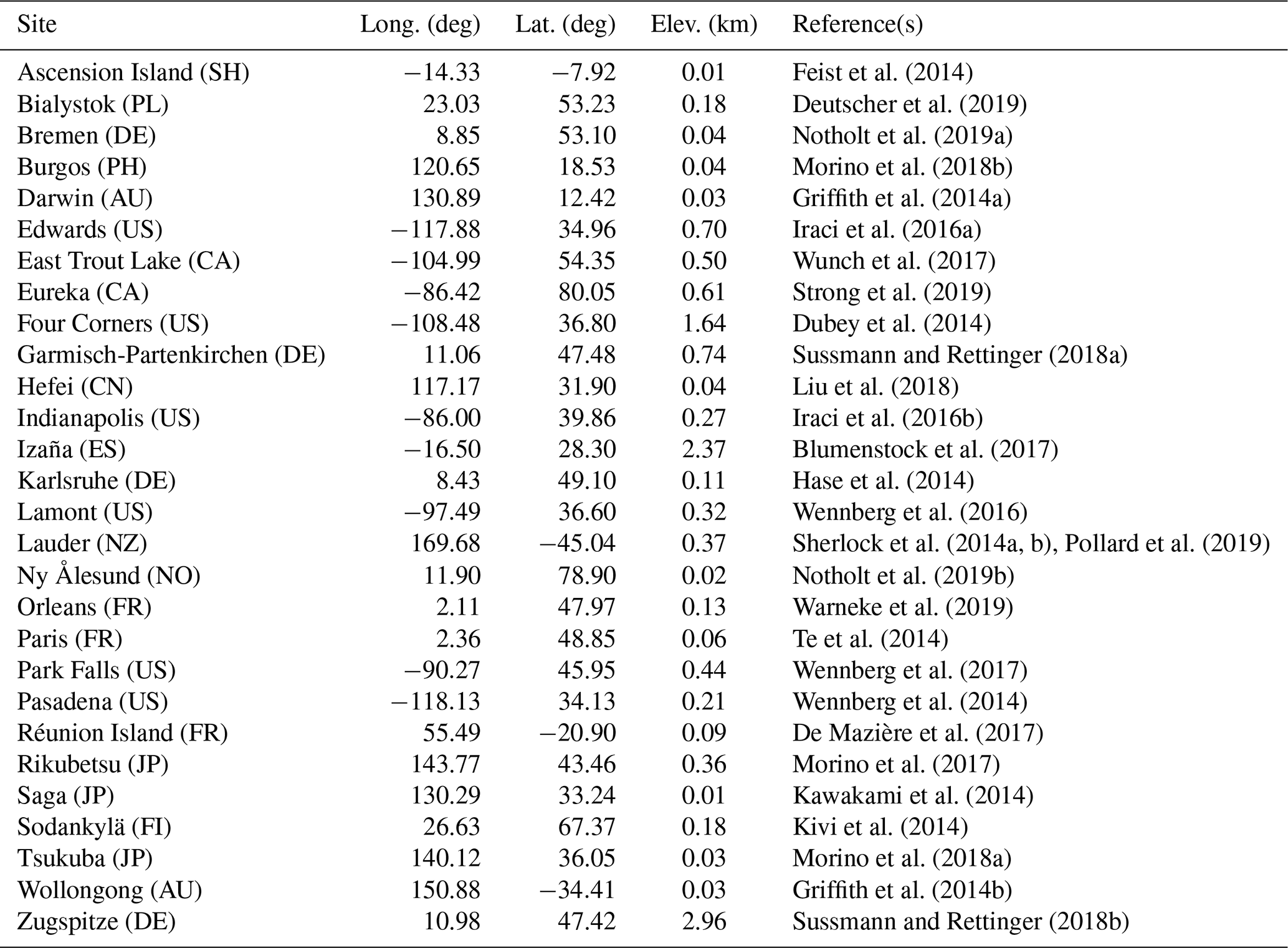
XCO2 a priori profiles are derived using the 2018 version of the simple empirical CO2 model SECM (Reuter et al., 2012). In the context of validation, we use the 2020 version of SECM. XCH4 a priori data are from the simple CH4 climatological model SC4C2018 developed and used by Schneising et al. (2019) and briefly described by Reuter et al. (2020).
For CO2 we use the “synth” a priori error covariance matrix described by Reuter et al. (2017b). For H2O, we use the same error covariance matrix as Reuter et al. (2017b), but scaled by a factor of 5 to reduce the dependencies of the retrieval results on the a priori. For CH4, for convenience, we scale the CO2 matrix to result in an XCH4 uncertainty of 45 ppb, which is considered to be a reasonable estimate. Note that only the matrices are scaled, not the a priori values.
2.3 The reference database
Quality filtering and bias correction usually require knowledge of a “true” (in this case XCO2) value. For this, we do not simply use model data as truth, as one aim of XCO2 products is to improve models. Another method is to take ground-based TCCON measurements as a basis for bias correction. However, although TCCON measurements are very accurate (estimated 1σ precision is 0.4 ppm; see Wunch et al., 2010), they are only available at certain locations and are therefore more suited for validation.
Our choice is therefore to use a database generated from a combination of TCCON measurements and CarbonTracker (CT) model data for a reference year (2018 for GOSAT, 2019 for GOSAT-2), which should on average reproduce large-scale features correctly.
This database is produced in the following way: as a first step, we determine from the CT data global daily 3D maps close to 13:00 local time (i.e. GOSAT and GOSAT-2 Equator crossing time). We reduce the altitude grid to five layers with the same dry-air sub-columns, i.e. the same quantity of particles, and interpolate the data from the native CT horizontal resolution of to . Then we determine from the TCCON data for each day mean values () for 13:00±2 h local time. Next, we select collocated CT data and correct them for the TCCON averaging kernels, resulting in a TCCON-corrected CT value at the TCCON location (). The application of the averaging kernels corrects for different vertical resolutions and/or sensitivities (see e.g. Rodgers and Connor, 2003; Wunch et al., 2010). We look for contiguous regions where CT XCO2 data differ by less than 0.75 ppm from the CT value at the TCCON location; these data are then used for the reference database. The reference database therefore does not contain any TCCON data – it only contains CT data which were confirmed by TCCON, but individual values may differ by up to 1.5 ppm. The choice of the 0.75 ppm ranges is based on a trade-off between accuracy (agreement with TCCON) and spatial coverage of the database.
The results are daily maps containing CO2 data for five vertical sub-layer altitudes. The spatial coverage is usually not global and varies from day to day. There are typically more data in the Southern Hemisphere during the second half of the year compared to the first half of the year (see Fig. 1). When comparing with GOSAT or GOSAT-2 measurement results, the true XCO2 is then computed from the CO2 layers of the reference database considering the retrieval's averaging kernels.
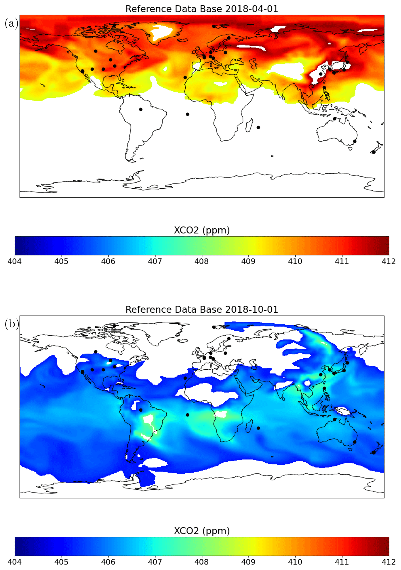
Figure 1XCO2 from the GOSAT-FOCAL reference database. The black markers show the locations of TCCON stations. (a) 1 April 2018. (b) 1 October 2018.
Specifically, for GOSAT we use CT2019 data in combination with TCCON GGG2014 (see Table 1) for 2018 here. For GOSAT-2 we also use TCCON GGG2014 data, but need to rely on CT-NRT v2020-1 for 2019. Because the CT NRT data are not yet available for the whole year of 2019, the GOSAT-2 reference database does not cover the whole year; there are essentially no data after August 2019. This is a limiting factor for GOSAT-2, especially because this also means that data in the Southern Hemisphere are less present in the 2019 database.
2.4 GOSAT Level 2 products
To assess the quality of the newly created GOSAT-FOCAL XCO2 products, they have been compared with several other well-established GOSAT Level 2 data sets (see Sect. 5). The GOSAT BESD v01.04 product from IUP (Heymann et al., 2015) is a near-real-time product generated in the context of the Copernicus Atmospheric Monitoring Service (CAMS, https://atmosphere.copernicus.eu/, last access: 30 July 2020) project. It is available from 2014 onward. The GOSAT RemoTeC v2.3.8 product from SRON (Butz et al., 2011) and the full-physics GOSAT product from the University of Leicester v7.3 (Cogan et al., 2012) were generated in the context of the Copernicus Climate Change Service (C3S, https://climate.copernicus.eu/, last access: 30 July 2020) and cover the GOSAT time series from 2009 until the end of 2019. The recently released NASA GOSAT ACOS v9r product (O'Dell et al., 2012, 2018; Kiel et al., 2019) is also available for the years 2009 to 2019. The operational GOSAT XCO2 product v02.95 (bias corrected) from NIES (Yoshida et al., 2013) currently ends in August 2020. The BESD product contains only XCO2 data over land; all other products are available for water and land surfaces.
The retrieval is performed in three main steps: pre-processing, processing, and post-processing. These are described in the following subsections.
3.1 Pre-processing
During pre-processing all required input data for the main processing step are collected. Furthermore, a first filtering of data is performed to reduce processing time.
The pre-processing procedure is largely based on the pre-processing as present in the BESD GOSAT product (Heymann et al., 2015). The sequence of pre-processing activities is as follows.
-
Extract measured spectra, geolocation, and information on quality and measurement modes (e.g. gain, scan direction) from the GOSAT L1B product.
-
Estimate instrument noise and cloud parameters.
-
Filter for data quality, latitudes, solar zenith angle, signal-to-noise ratio, and clouds (see Table 2 for settings).
-
Extract surface type, elevation, and roughness derived from the surface database for each measurement.
-
Add corresponding meteorological information (pressure, temperature, dry-air column, and water vapour profiles) for the time and place of the measurements. This includes a correction for surface elevation; i.e. model profiles are extended or cut according to the value from the surface database.
-
Add a priori gas profiles for each measurement (CO2 from SECM, CH4 from SC4C, H2O from meteorology). For GOSAT-2, a priori profiles for CO and N2O are also added. The latter do not depend on geolocation; they are based on the tropical reference atmosphere from Anderson et al. (1986), scaled to column average values of XCO =0.1 ppm and XN2O =330 ppb.

Because FOCAL is a fast algorithm and the number of GOSAT and GOSAT-2 measurements is much lower than for OCO-2, we chose to set the pre-processing filters to be relatively relaxed and to apply the quality filtering mostly in the post-processing. As can be seen from Fig. 2 about two-thirds of the measurements are filtered out during pre-processing.
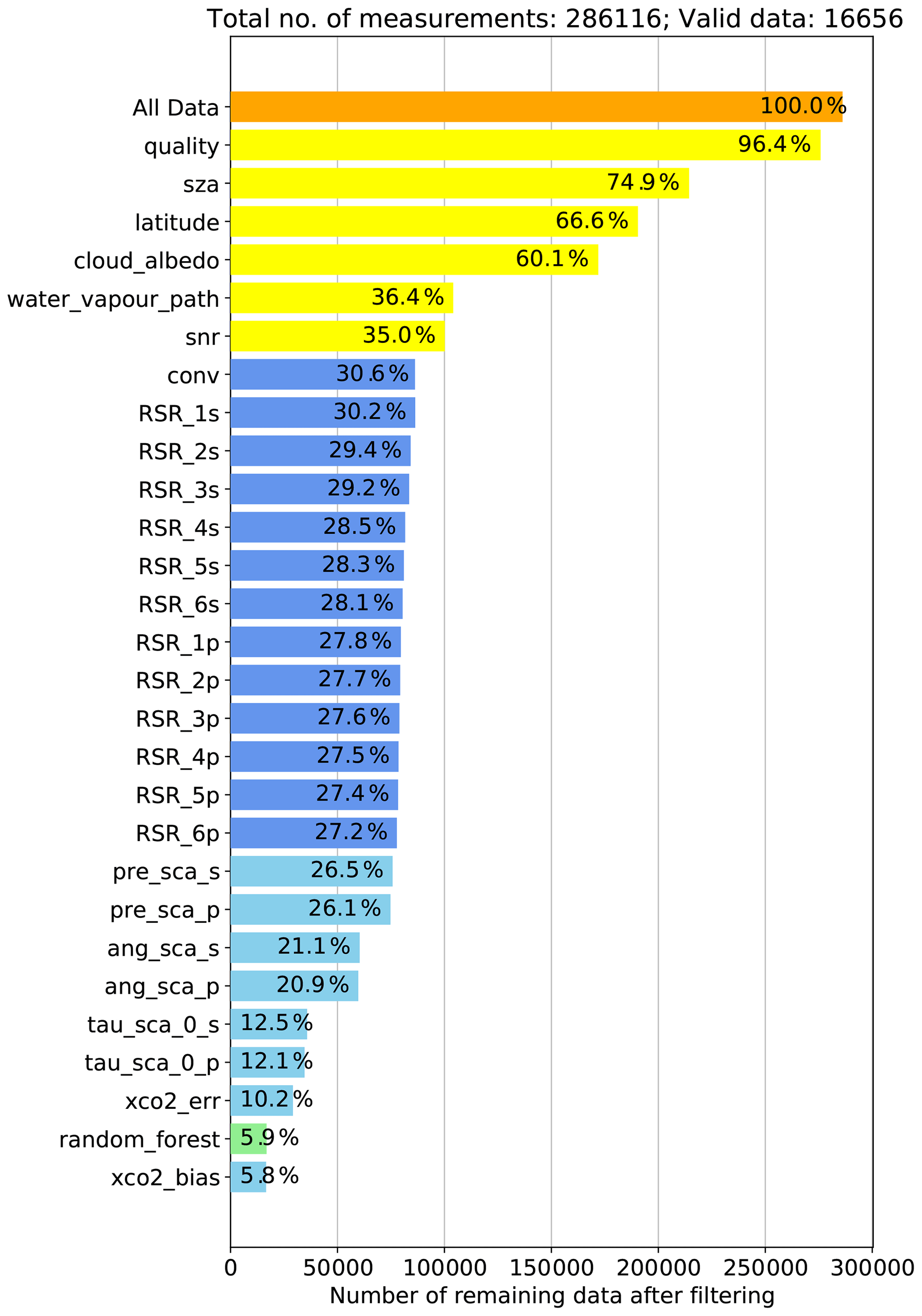
Figure 2Example for GOSAT data filtering during the different processing steps (April 2019). Filters are listed in sequential order from top to bottom on the vertical axis. Numbers in the horizontal bars denote the percentage of remaining data after this filter was applied. Orange: total number of measurements before filtering. Yellow: pre-processing filters. Blue: step 1 post-processing filters (convergence and noise). Green: random forest post-processing filter. Light blue: additional post-processing filters.
3.1.1 Noise estimate
Similar to Heymann et al. (2015) the spectral noise is initially assumed to be independent from the wavenumber for each band. It is estimated from the standard deviation of the real part of the “dark” off-band signal (i.e. the first 500 spectral points in each band). In a later step (see Sect. 3.2.1) this noise will be modified to account for additional forward model errors and overall scaling.
3.1.2 Cloud filter
The cloud filtering is based on two physical properties of clouds: clouds are (usually) bright and clouds are high (higher than the surface) so that little water vapour is above them. In the pre-processing these properties are described by two quantities: effective albedo and water vapour filter. These are derived for each spectrum as described in Heymann et al. (2015). The effective albedo for each band is estimated from the mean reflectance L within a spectral range outside the absorption. L is determined from the mean radiance I, the mean irradiance I0, and the solar zenith angle α via
The specific wavenumber ranges and irradiance values used for filtering are given in Table 3.
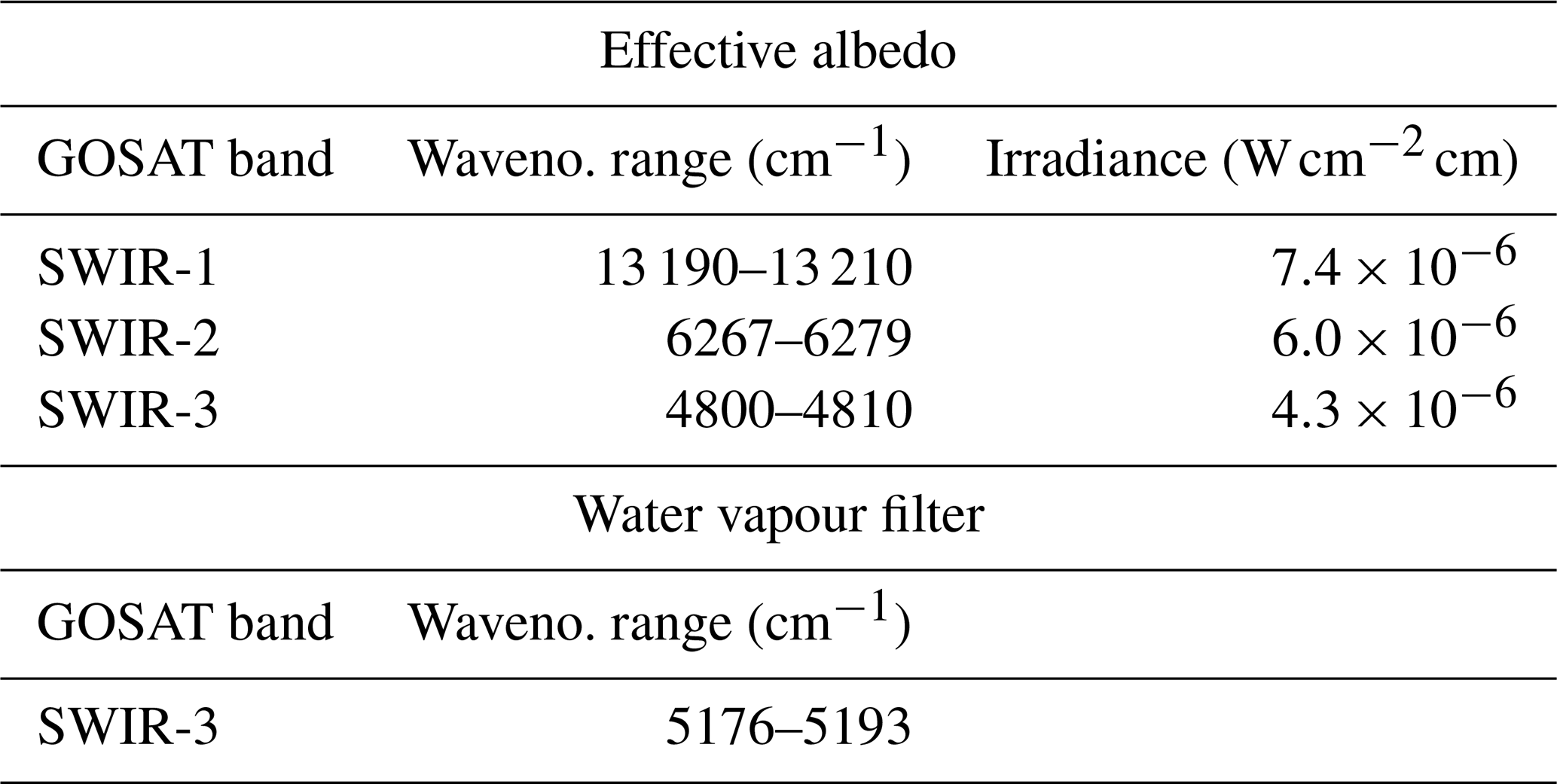
The water vapour filter is determined from a spectral region with strong water vapour absorption in the SWIR-3 band (see Table 3). This filter is defined as the ratio between the median radiance and the median of the estimated noise in this spectral range.
A ground pixel is assumed to be cloudy if either the effective albedo in one of the bands or the water vapour filter exceeds the thresholds given in Table 2.
3.2 Processing
The processing is based on the Fast atmOspheric traCe gAs retrievaL (FOCAL) algorithm, which is described in detail in Reuter et al. (2017c). A first successful application of this algorithm to OCO-2 data is given in Reuter et al. (2017b). Therefore, we only summarise the main features of the algorithm here and point out the differences to the OCO-2 application.
FOCAL approximates modifications of the direct light path due to scattering in the atmosphere by a single scattering layer, which is characterised by its height (pressure level), its optical thickness, and an Ångström parameter that describes the wavenumber dependence of scattering. The layer height is normalised to the surface pressure. Furthermore, Lambertian scattering on the surface is considered. For atmospheric scattering processes an isotropic phase function is assumed. With this approximation, the FOCAL forward model is essentially an analytical formula; it uses pre-calculated and tabulated cross sections such that calculations can be performed considerably fast. The inversion of the forward model is based on optimal estimation (Rodgers, 2000) and uses the Levenberg–Marquardt–Fletcher method (Fletcher, 1971) to minimise the cost function.
The OCO-2 retrieval of Reuter et al. (2017b, c) uses four fit windows in the NIR (near-infrared) and SWIR spectral range to derive the atmospheric parameters XCO2, water vapour, and SIF. In contrast to OCO-2, GOSAT and GOSAT-2 cover a wider spectral range and provide spectra in two polarisation directions referred to as S and P. Therefore, we treat both polarisation directions as independent spectra in our retrieval as opposed to the average of both as usually used in other GOSAT retrievals (see e.g. Butz et al., 2011; Cogan et al., 2012; O'Dell et al., 2012). However, recently Kuze et al. (2020) presented a methane retrieval for GOSAT based on an algorithm from Kikuchi et al. (2016), which also makes use of both polarisation directions.
We use both polarisation corrections mainly for the following reasons.
-
In principle, information is lost when averaging S and P spectra.
-
In general, the sensitivity of the instruments and therefore the calibration of the measured spectra is different for S and P. For example, the measured ILS is given independently for S and P.
-
S and P include different information on scattering, which can also be used in filtering and/or bias correction.
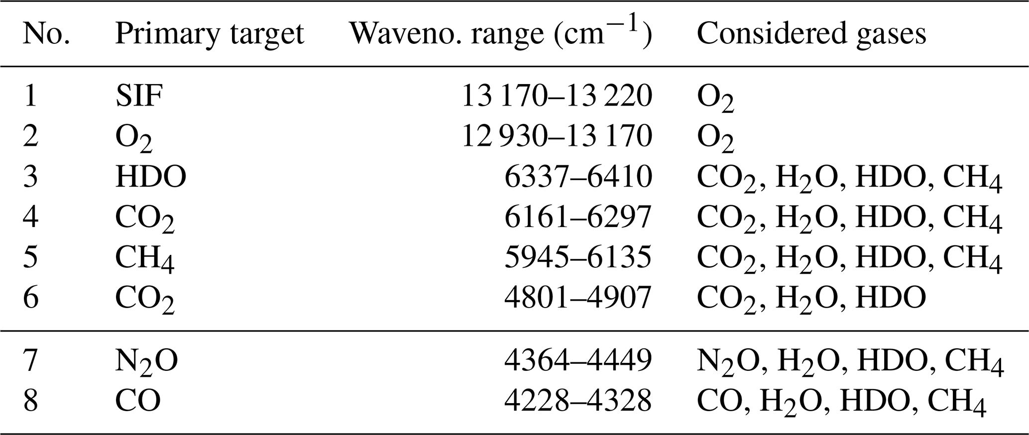
Furthermore, the FOCAL fitting windows (see Table 4) have been adapted to the specific GOSAT(-2) spectral bands such that, in addition, other atmospheric constituents and parameters like HDO can be derived. In the case of GOSAT-2, XN2O and CO total columns can also possibly be retrieved. This results in six fitting windows for GOSAT and eight windows for GOSAT-2 for each polarisation. The retrieval is performed on a wavenumber axis.
Table 4Definition of GOSAT and GOSAT-2 spectral fit windows (same for S and P). Windows 7 and 8 are only available for GOSAT-2.
Because of the large number of target gases and spectral bands the retrieval requires various state vector elements. These are listed together with the fit windows, from which they are determined, and their a priori values and uncertainty ranges in Table 5 for GOSAT and GOSAT-2.
Table 5State vector elements and related retrieval settings. A priori values are also used as a first guess. “Fit windows” lists the spectral windows (see Table 4) from which the element is determined. “All” means that an element is determined from all fit windows of the specified polarisation. “Each” means that a corresponding element is fitted in each fit window. A priori values labelled “PP” are taken from pre-processing; “est.” denotes that they have been estimated from the background signal.
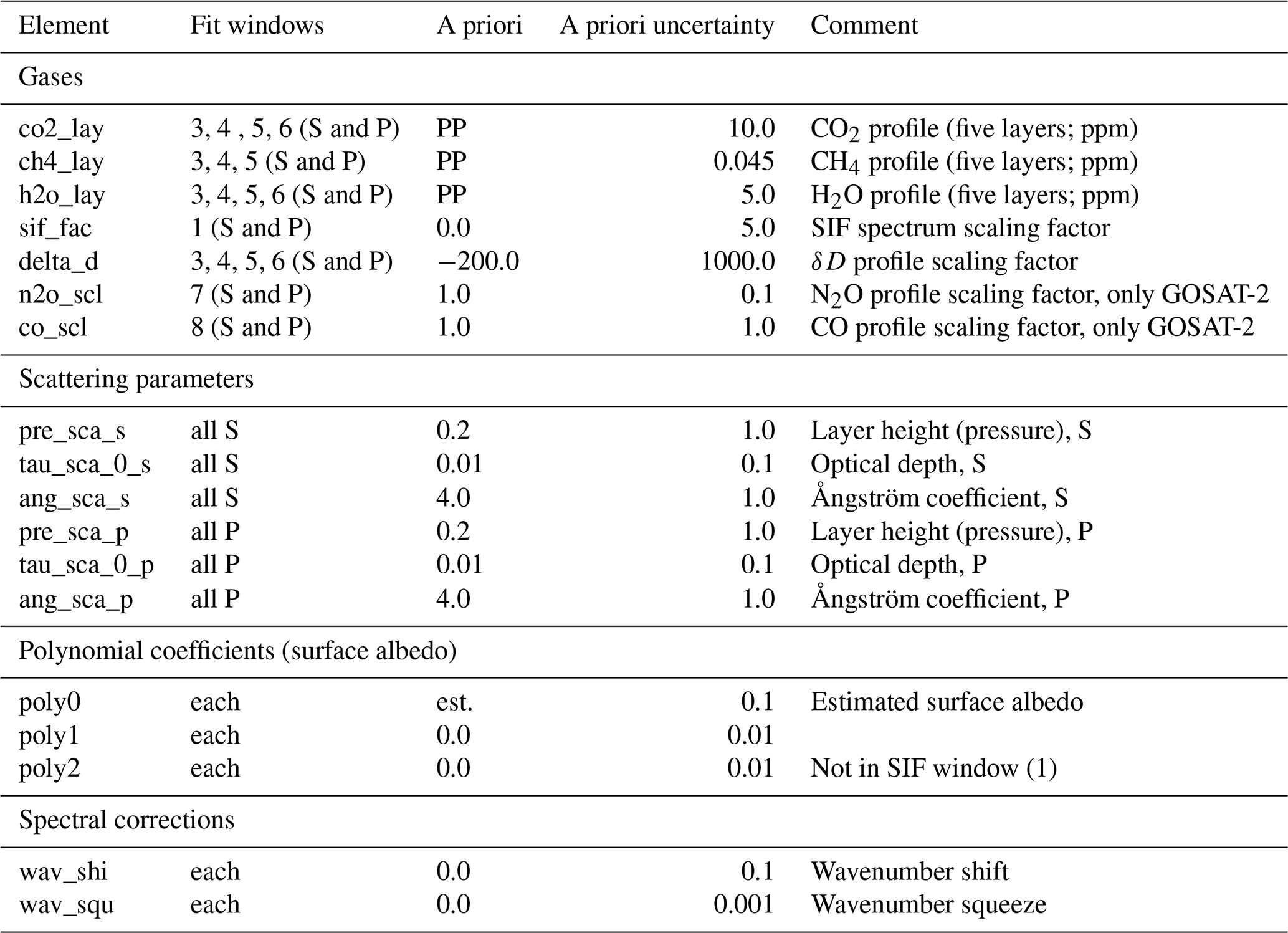
Note: for GOSAT-2 the polynomial degree in fit window 1P is (accidentally) set to 2 and in fit window 7S to 1.
For GOSAT, the retrieval determines CO2, CH4, and H2O on five layers with same number of air particles, from which the column average values XCO2, XCH4, and XH2O are then calculated. Furthermore, solar-induced fluorescence (SIF) is determined by scaling a corresponding reference spectrum.
Instead of the HDO column, we fit a scaling factor for the relative abundance of HDO compared to H2O, δD, which is defined as
where Rmeas is the ratio of the measured HDO and H2O columns, and RVSMOW () is the corresponding value for Vienna Standard Mean Ocean Water (VSMOW). δD is usually given in units of per mill.
δD=0 ‰ corresponds to HDO concentrations as in VSMOW and ‰ to no HDO. We assume the same profile shape for HDO as for H2O. For GOSAT-2, we also fit scaling factors to (fixed) CO and N2O profiles.
As mentioned above, atmospheric scattering is considered in FOCAL by a single scattering layer, which is described by three parameters (height, optical depth, and Ångström coefficient). As scattering is different for S- and P-polarised light, we fit two independent layers for S and P.
In addition, we determine in each fit window (independently for S and P) a polynomial background function describing the surface albedo. For this we use second-order polynomials except for the small SIF windows (no. 1) for which a linear function is sufficient. Note that in the current version of the GOSAT-2 product the polynomial degree in fit window 1P is accidentally set to 2 and in fit window 7S to 1. This has no major impact on the retrieved XCO2 and will be corrected in a future product version.
The GOSAT data files only contain a fixed spectral axis. As described in e.g. Heymann et al. (2015), the spectral calibration of GOSAT changes with time, especially at the beginning of the mission. This change can be corrected by a spectral scaling factor. We determine this overall scaling factor by a spectral fit in the SIF window before the retrieval. So far, this spectral pre-fitting seems to be unnecessary for GOSAT-2. In the retrieval, we then additionally consider for both GOSAT and GOSAT-2 possible additional spectral shifts and squeezes in each fit window by corresponding state vector elements, but the influences of these spectral changes on the results is rather small.
Noise model
The noise N derived from the off-band signal is only an estimate. It does not consider a possible wavenumber dependence of the noise within one spectral band. Furthermore, a potential error of the forward model needs to be considered. In the optimal estimation method this can be achieved by including the forward model error in the measurement error covariance. For this, we define a scaling factor s for the estimated noise and the quantity δF, which denotes the relative error of the forward model. The forward model error is proportional to the continuum radiance outside the absorption I, which is estimated from the 0.99 percentile of the measured radiance at the edge of each fit window. The quantities δF and s are determined using the approach described in Reuter et al. (2017b), i.e. by running the retrieval for a representative subset of data and then fitting the function
to binned values of the residual-to-signal ratio (RSR) as a function of the noise-to-signal ratio (NSR). RSR is defined as the standard deviation of the retrieved spectral residual in each fit window divided by the continuum signal I; NSR is the standard deviation of the noise divided by I.
With the method described in Reuter et al. (2017c) it is also possible to define a 2σ outlier limit based on NSR and RSR data, which will be used to filter out data that are too noisy during post-processing (see Sect. 3.3). This is parameterised by a second-order polynomial as a function of the uncorrected NSR:
which is added to the RSR function of Eq. (3). The coefficients ai are determined via a fit. To avoid extrapolation, fN is set to the edge values outside the fitting range.
In order to cover the varying signal over the year, we base the noise model fits on data from 1 d per month for one reference year. For GOSAT, we take data from December 2017 to November 2018 (as there are few GOSAT data available in December 2018). For GOSAT-2 we use data from February 2019 to December 2019. In the case of GOSAT-2 we further restrict the input data for the noise model parameter fit to data over land because some of the data over water show an unexpected behaviour (low RSR in the case of large NSR), which needs further investigation. In this sense, the current GOSAT-2 noise model is considered to be preliminary and may need some refinement in the future.
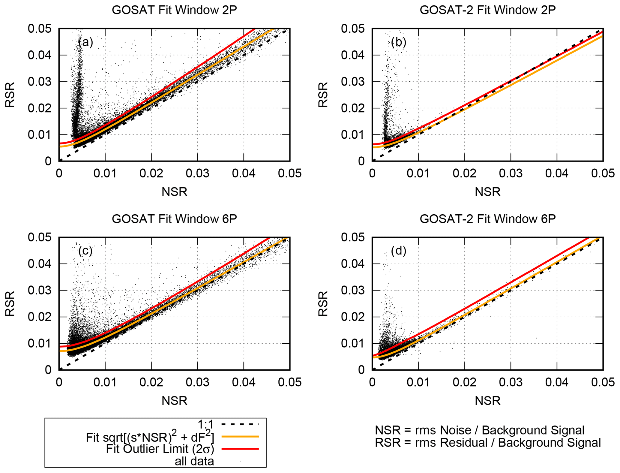
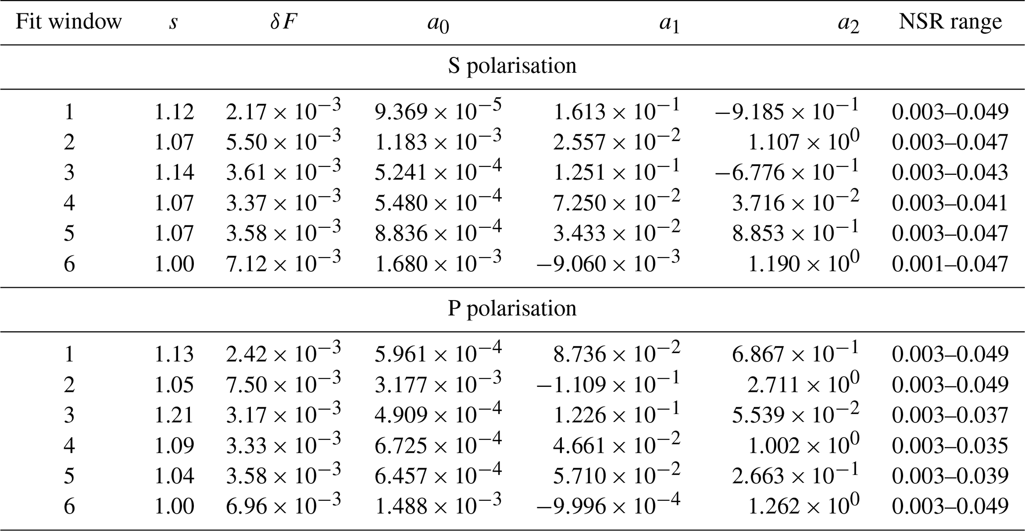
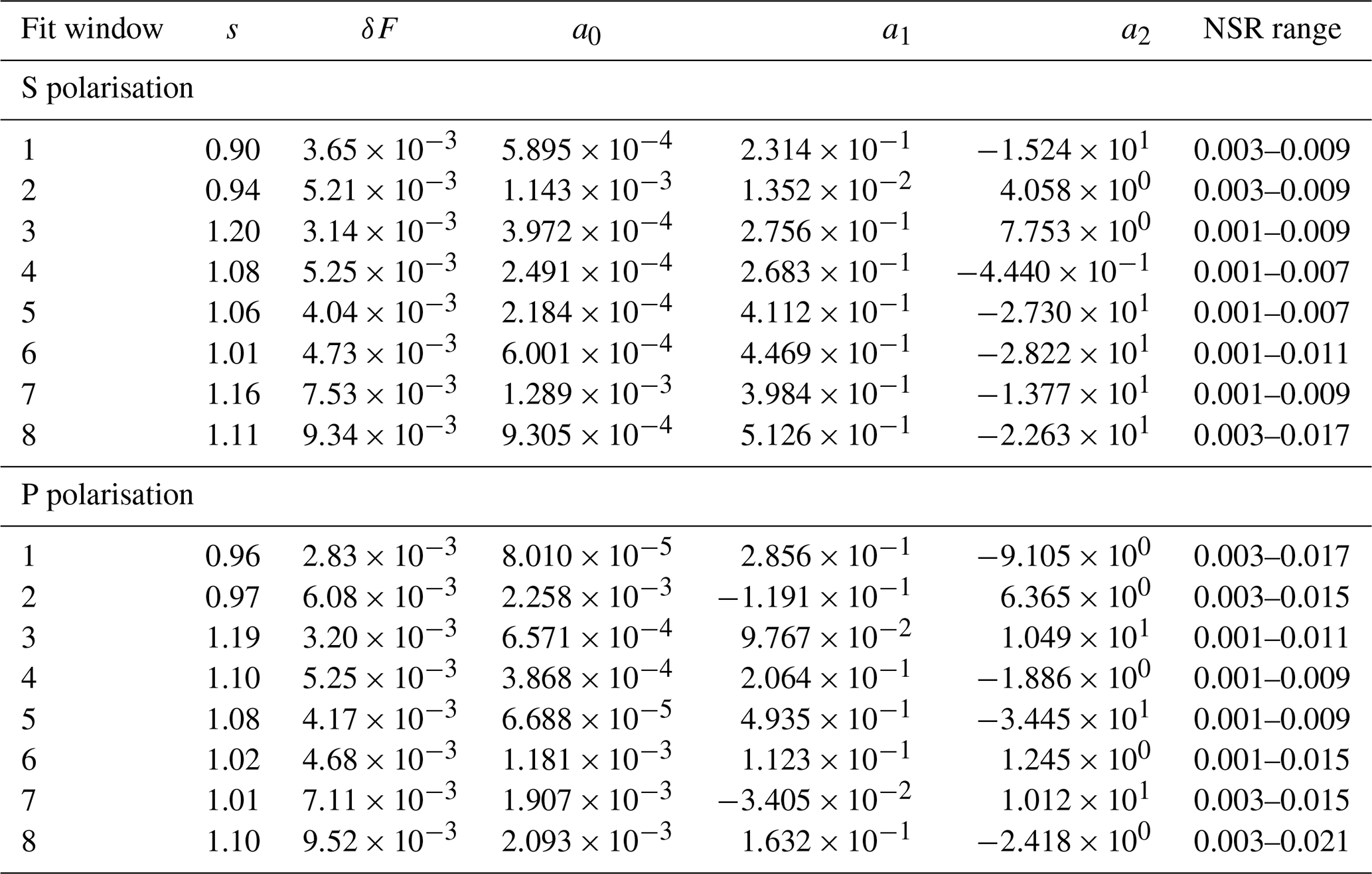
Figure 4Example results from the noise model. (a) GOSAT fit window 2P. (b) GOSAT 2 fit window 2P. (c) GOSAT fit window 6P. (d) GOSAT 2 fit window 6P.
Figure 4 shows as an example the noise model results for GOSAT and GOSAT-2 in the fit windows 2 (O2(A) band) and 6 (strong CO2 absorption) for P polarisation. The orange line gives the fitted RSR function and the red line the outlier limit. The derived values from the noise model for all fitting windows and polarisations are given in Tables 6 and 7 for GOSAT and GOSAT-2. The forward model errors δF are on average slightly larger for GOSAT-2 than for GOSAT. In the SWIR, values similar to OCO-2 are obtained, but in the NIR the OCO-2 δF is typically smaller (about 0.003). This indicates that for GOSAT and GOSAT-2 instrumental and/or calibration effects seem to impact the radiance errors more in the NIR than in the SWIR.
3.3 Post-processing
The purpose of post-processing is to filter out invalid data and to perform a bias correction for the products. The current post-processing focuses on XCO2. The post-processing is performed in several steps, namely the following:
-
basic filtering based on physical knowledge;
-
filtering out low-quality data using parameters and limits determined with a random forest classifier;
-
application of a bias correction using a random forest regressor; and
-
additional filtering-out of data with a bias correction that is too large.
These steps are described in the following subsections.
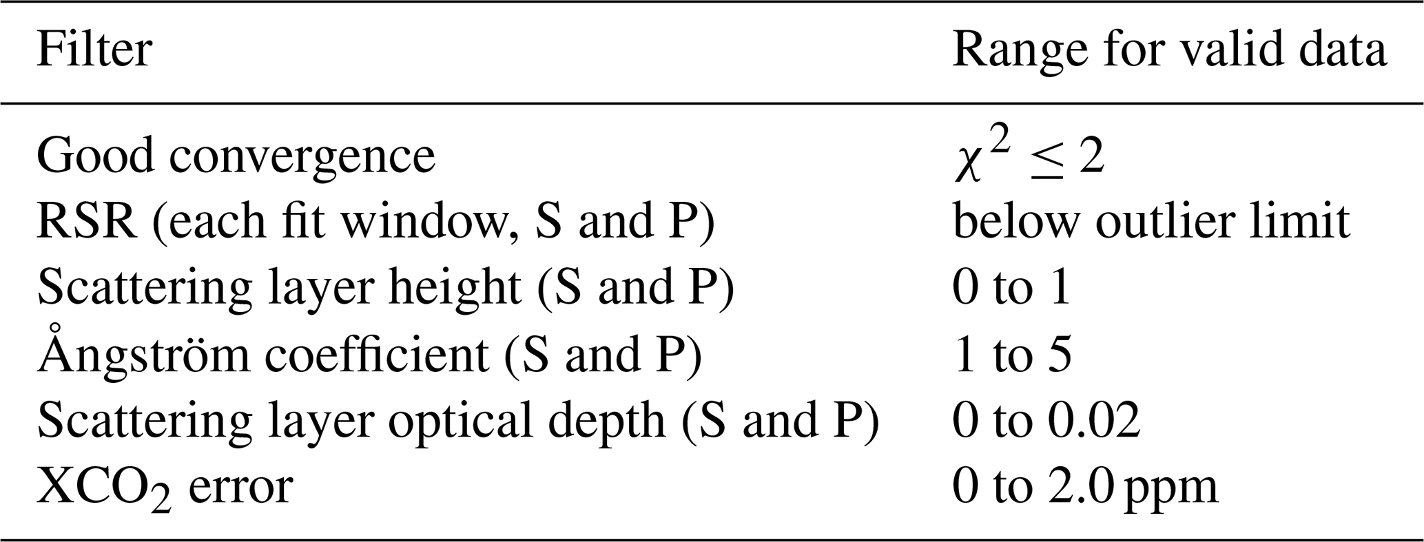
3.3.1 Basic filter
The basic filtering removes measurements for which the retrieval does not converge or for which the quality of the fit results is too low. We consider this to be the case if the χ2 calculated over all fit windows is larger than 2 or if for at least one of the fit windows the RSR outlier limits (see Sect. 3.2.1) are exceeded. Furthermore, we apply some initial filters for nonphysical values to the derived scattering parameters (i.e. layer height outside the atmosphere, Ångström coefficient not within [1,5]). Note that all retrieved scattering parameters such as the Ångström exponent can be considered “effective” parameters as they have to account for not only cloud–aerosol scattering but also Rayleigh scattering (which has an Ångström coefficient of 4). Because Rayleigh scattering is always present and we filter out cloudy scenes, we usually get higher effective Ångström coefficients than those expected from clouds or aerosols only.
We also limit the maximum allowed optical depth of the scattering layer to 0.02 to filter out clouds or aerosol amounts that are too thick and use a maximum allowed XCO2 posteriori uncertainty of 2 ppm. As described by Reuter et al. (2017c), FOCAL simulates scattering only for an isotropic phase function. The prominent forward peak, usually existing for Mie scattering phase functions of cloud and aerosol particles, basically does not modify the light path. As FOCAL's optical depths of the scattering layer do not include this forward peak, these optical depths are much smaller than optical depths including a strong forward peak while having a similar influence on the light path modification (see discussion in the publication of Reuter et al., 2017c). The maximum value of 0.02 for the layer optical depth should therefore not be interpreted as e.g. an aerosol optical depth.
The limits for the optical depth of the scattering layer and the XCO2 error are somewhat arbitrary and actually result from visual inspection of the retrieval results. However, they are only intended as a first rough quality filter to facilitate later filter and bias correction methods, which will partly use the same parameters (see below). The detailed choice of these limits is therefore considered uncritical for the final results.
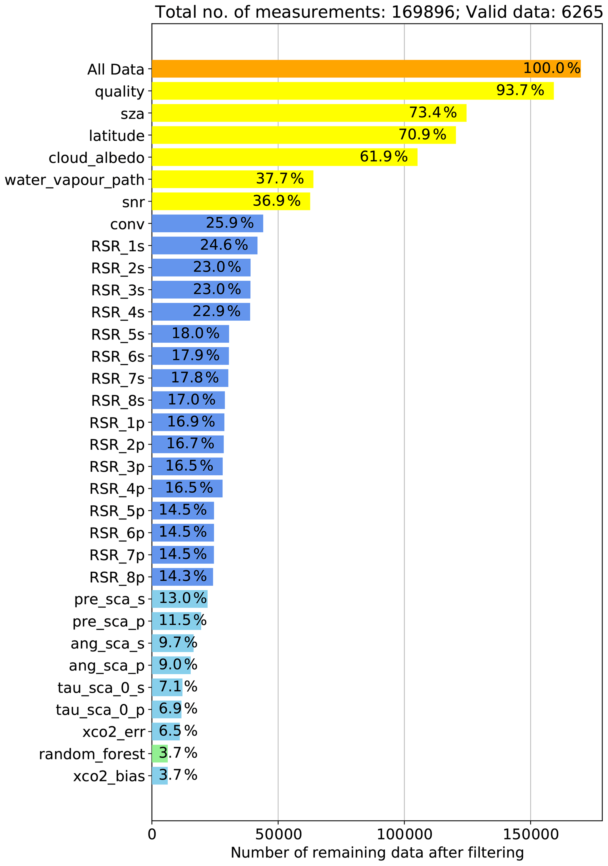
The above-mentioned filter parameters and limits (see Table 8) are applied to both land and water surfaces and are the same for GOSAT and GOSAT-2 except for the RSR outlier limit, which has been determined individually for each instrument. Figures 2 and 3 show how many data points are typically filtered out in this step. The different performance of the RSR filters for both instruments indicates that the filtering for GOSAT-2 needs some further optimisation, which is planned for the next version of the products.
3.3.2 Random forest filter
In the next step, data are filtered out based on their expected XCO2 bias, i.e. the difference to a true XCO2. Of course, this true XCO2 value is normally not known. We therefore use the XCO2 reference database (as described in Sect. 2.3) to train a random forest classifier (Pedregosa et al., 2011) to identify those variables which would remove – in combination with a corresponding random forest database – a pre-described percentage p of data based on their XCO2 bias. This is done independently for data over land and water. Note that we are only interested here in the XCO2 bias on top of an overall global bias as the latter will be handled via the bias correction.
This method is similar to the random forest filter used by Schneising et al. (2019) in the context of CH4 and CO retrieval. Other approaches for data filtering used e.g. by Mandrake et al. (2013) and Reuter et al. (2017b) identify the best variables through the minimisation of local XCO2 variability in the retrieved products. However, all methods essentially serve the same purpose, i.e. to derive a reproducible filtering procedure which does not solely rely on expert knowledge.
We determine the list of relevant variables and the random forest database for the filtering in the following way: we use the (uncorrected) results of the retrieval for the reference and apply the basic filtering as described in Sect. 3.3.1. Then, the subset of these data is selected which has a corresponding true value in the reference database. For these data we determine the XCO2 bias (measurement – reference XCO2) and subtract the global median for land and water of this bias. We then sort the data according to this bias and flag those p percent of data with the highest absolute bias values as “bad”.
For GOSAT, this results in a total of 54 317 data points over land and 109 414 over water. These numbers are smaller for GOSAT-2 (land: 10 625, water: 40 459). The random forest classifier is then trained by randomly using 90 % of these data as input. The training is done in two iterations: first with a complete set of possible input variables (“features”) and output variables (“estimators”) and then using only a reduced set consisting of the 10 best features and/or estimators, i.e. those with the highest random forest score (relevance) in the first run. This relevance is a quantity which describes the relative importance of each feature for the filtering. Relevances are normalised such that the sum of all relevances is 1. The random forest classifier then decides for each measurement based on these 10 variables if it is filtered out or not.
The initial list of possible features and estimators essentially includes all quantities available after the retrieval, including viewing angles, surface properties, and the continuum signal for each fit window. Furthermore, the retrieved values of the state vector elements and their errors are included in this list as are averaging kernels for the profiles. We explicitly exclude the geolocation of the measurement (latitude, longitude) and the retrieved values (but not the errors) for the data products we are interested in, i.e. the gases and SIF. This is to avoid e.g. the filtering-out of certain geographical regions or removing all points with high XCO2 values.
Note that in glint mode over ocean, the inclusion of information about the viewing geometry as possible features bears the risk that the random forest procedure may infer the geolocation from a combination of these.
However, we include as a possible filter variable the gradient of the retrieved CO2 profile (i.e. the difference between the two lowermost layers) as this has shown to be a suitable quantity.
The original number of candidate variables presented to the random forest classifier is quite high (193 for GOSAT and 246 for GOSAT-2) as can be seen from Figs. 5 and 6 (top left plots), but there are few with high relevance.
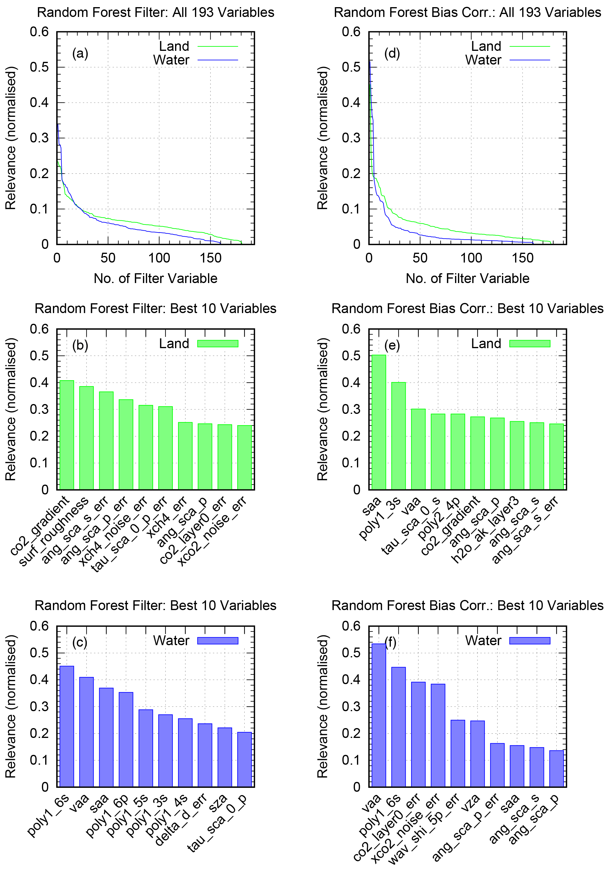
Figure 5Random forest results for GOSAT. (a–c) Results from the random forest filter. (d–f) Results from random forest bias correction. (a, d) Normalised relevance (score) of all filter variables. (b, e, c, f) Selected variables and their relevance for the land and water surfaces.
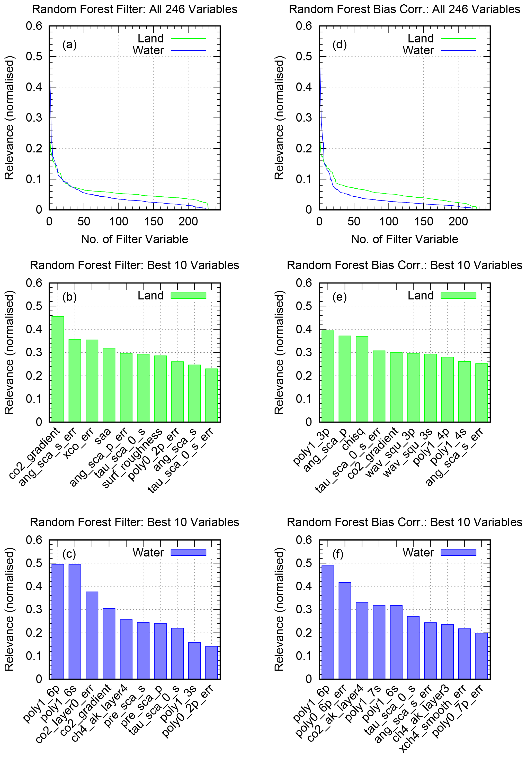
The 10 best variables selected partly differ for land and water surface (as shown in the middle and left top panels), but they usually comprise scattering parameters, polynomial coefficients, spectral corrections, and some XCO2-related parameters.
The other 10 % of the input data are used to test the performance of the classifier. The results from this test and other cross-validation activities indicate that the random forest classification is – depending on surface – only accurate in about two-thirds of the cases. This accuracy is defined as the fraction of correctly classified samples. This means that the filtering also removes possibly valid data points and does not remove all possibly bad ones. However, we do not expect a perfect classification because it is not possible to describe all inter-dependencies via the set of input features. Note that the performance of the filter is similar for both the training and the test data sets. This indicates that there are no problems with over-fitting.
To obtain high quality of the remaining XCO2 data, we therefore need to filter out quite a large percentage of data (and perform an additional filtering at a later time; see below). For future data products further investigations are planned to improve the performance of the classifier, e.g. by providing additional features from the combination of existing ones (like the already used CO2 gradient). The percentage p of data to be filtered out is usually a trade-off between data quality and the remaining amount of data. In the present case a 50 % limit has been selected. Actually, as can be seen from Figs. 2 and 3, the relative amount of data filtered out via the random forest classifier is not exactly 50 % of the data remaining after the previous filters.
3.3.3 Bias correction and filtering
XCO2 retrieval methods usually require a bias correction to be applied to the data. This correction is often based on multi-linear regressions using parameters identified from correlation analyses of differences to an assumed true XCO2 data set. Different data products use different methods to define this “truth”. In many cases, ground-based TCCON measurements are taken as a reference for the true XCO2, like in the GOSAT BESD product (Heymann et al., 2015), the SRON products (Guerlet et al., 2013), the product from the University of Leicester (Cogan et al., 2012), and also the operational GOSAT product from NIES (Inoue et al., 2016). The bias correction of the NASA ACOS OCO-2 product is quite complex (O'Dell et al., 2018; Kiel et al., 2019); it uses as a reference a modification of the Southern Hemisphere approximation introduced by Wunch et al. (2011b). The ACOS product takes multi-model mean data as a reference and derives corrections from data in the Southern Hemisphere below 20∘ S where CO2 is assumed to be quite uniform in small areas. A similar small area approximation is also used by Reuter et al. (2017c) to correct FOCAL OCO-2 data. This correction method is not possible for GOSAT and GOSAT-2 data because of their sparse sampling. We therefore follow a different approach here.
For the bias correction we use as input the same data set as for the random forest filter, but with this random forest filter applied; 50 % of the resulting data set is then used to train a random forest regressor (see also Schneising et al., 2019), which aims to minimise the true XCO2 bias, i.e. the difference to the reference database value without the global median subtracted, as a function of the specified features. To create the bias correction database and the corresponding list of best features we again run the training twice, first with the full list (the same as for the filter) and then with the top 10 features. Again, we use different corrections for land and water. The resulting parameters and their performance are shown in the bottom panels of Figs. 5 and 6. The bias correction selects similar best features as the filter, but not exactly the same quantities in the same sequence.
The actual number of features and variables to be used for both filtering and bias correction is a trade-off between many variables (explaining all relations with a risk of over-fitting and high computational effort) and few variables (no over-fitting, but maybe missing some relations). Considering 10 features for the bias correction is more than other algorithms typically use, but this is appropriate in our case because we take into account the different relevance of these parameters, which drops off rapidly within the first 10 variables (see top panels of Figs. 5 and 6).
The validity of this choice is confirmed by the application of the bias correction to the training data set and the other 50 % of the input data, which shows a comparable reduction of the XCO2 scatter. This is an indication for a good performance (e.g. no over-fitting) of the regressor.
During application of the bias correction, the random forest regressor estimates the XCO2 bias based on the values of the input variables. This bias is then subtracted from the retrieved value.
Currently, there is only a bias correction for XCO2, but in principle this method is also applicable to other quantities depending on the availability of a corresponding reference database.
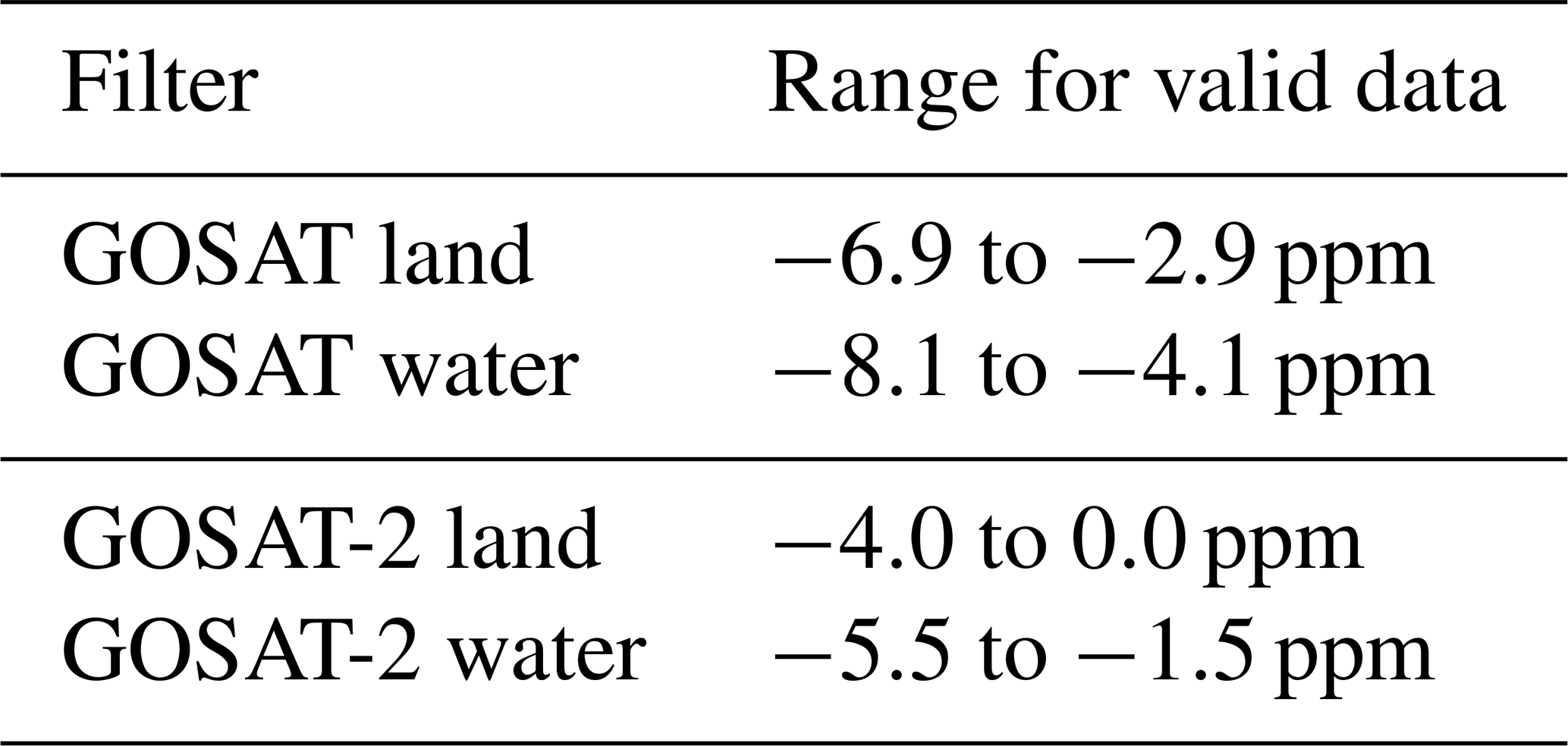
After the bias correction there are still a few outliers left in the XCO2 data. These are filtered out by an additional filter on the XCO2 bias derived via the random forest classifier. The limits for this filter are the global median bias for the test data set plus and minus 2 ppm. The median bias is different for land and water surfaces and also for GOSAT and GOSAT-2. The actual limits are given in Table 9. The value 2 ppm is estimated from visual inspection of the data. Figures 2 and 3 show that typically less than 1 %–2 % of the remaining data (less than 0.1 % of all) are affected by this last filter.
The spatial variability of the finally derived bias correction (see Fig. 7) is typically below 1 ppm, but as mentioned above there is a systematic difference between land and water data of about of 1–1.5 ppm (see Table 9).
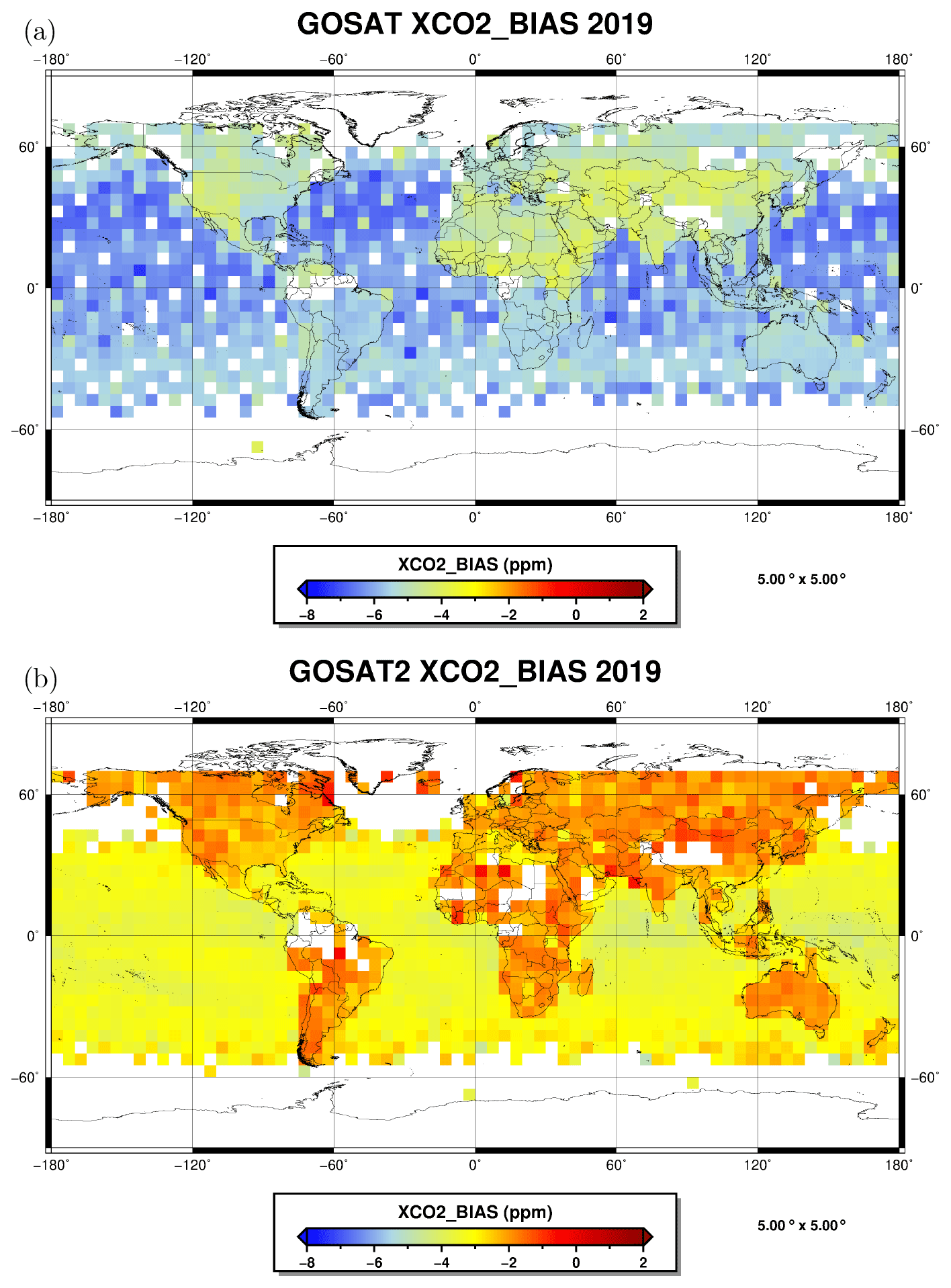
Figure 7Gridded GOSAT (a) and GOSAT-2 (b) XCO2 bias correction for 2019.
The FOCAL retrieval has been applied to all GOSAT and GOSAT-2 measurements until the end of 2019. On average, FOCAL needs 22 s with six iterations for the processing of one GOSAT ground pixel. For GOSAT-2 the numbers are slightly higher (28 s for seven iterations) because of the additional fit windows and state vector elements. All performance values are given for a single core of an Intel Xeon E5-2667v3 CPU (3.2 GHz). These numbers are actually about 1 order of magnitude larger than the ones given in Reuter et al. (2017b, c) for the FOCAL application to OCO-2. This is because we use separate S- and P-polarisation spectra and more retrieved variables for GOSAT(-2), which requires more and larger fit windows. For each of these fit windows and parameters, weighting functions have to be calculated, which involves a convolution with the ILS. This convolution is the most time-consuming part of the FOCAL retrieval. This is even more relevant for GOSAT(-2) because the FTS ILS is in principle sinc-shaped; i.e. it has a sharp peak in the centre but wide wings, which requires a large kernel width (in our case 15 cm−1) for the convolution.
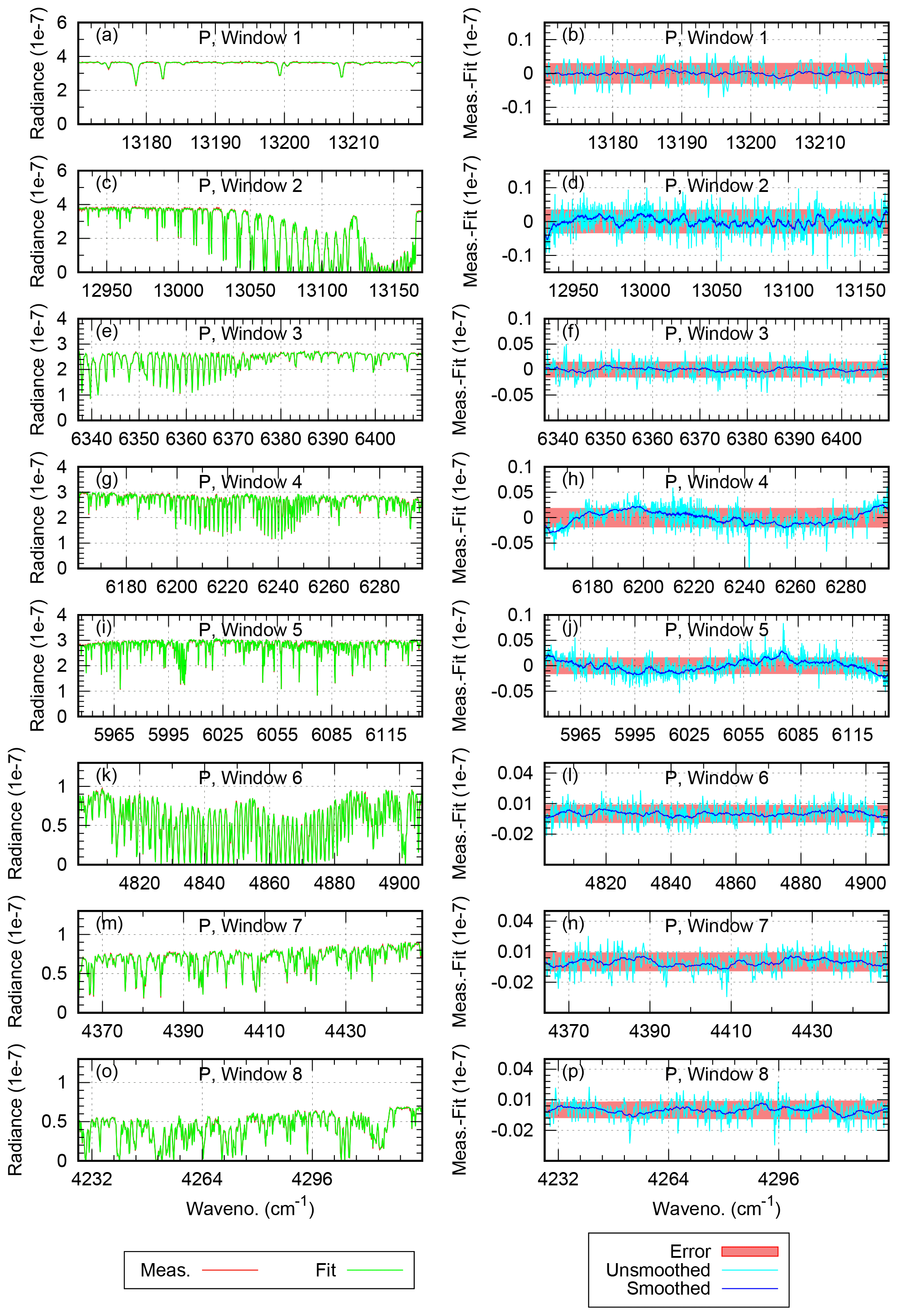
The left plots in Figs. 8 and 9 show examples for measured and fitted nadir-mode radiance spectra for GOSAT and GOSAT-2 over land in the different fitting windows for P polarisation. Since the difference between measured and modelled spectra is small and thus hard to see, we show in these figures on the right side the corresponding residuals and the estimated noise. The results for S polarisation look similar and are therefore not shown here. The residuals are on the order of magnitude of the noise, which is slightly higher for P polarisation than for S polarisation. Some small spectral structures are visible in the residuals; they appear more clearly in the smoothed residuals (convoluted with a 21-pixel boxcar), e.g. for GOSAT and GOSAT-2 in the O2(A) band (window 2), and some broadband oscillations in window 4 and 5 for GOSAT-2. These features are present in both S and P polarisations and also occur in other measurements, so they seem systematic. A reduction of these features could further improve future products.
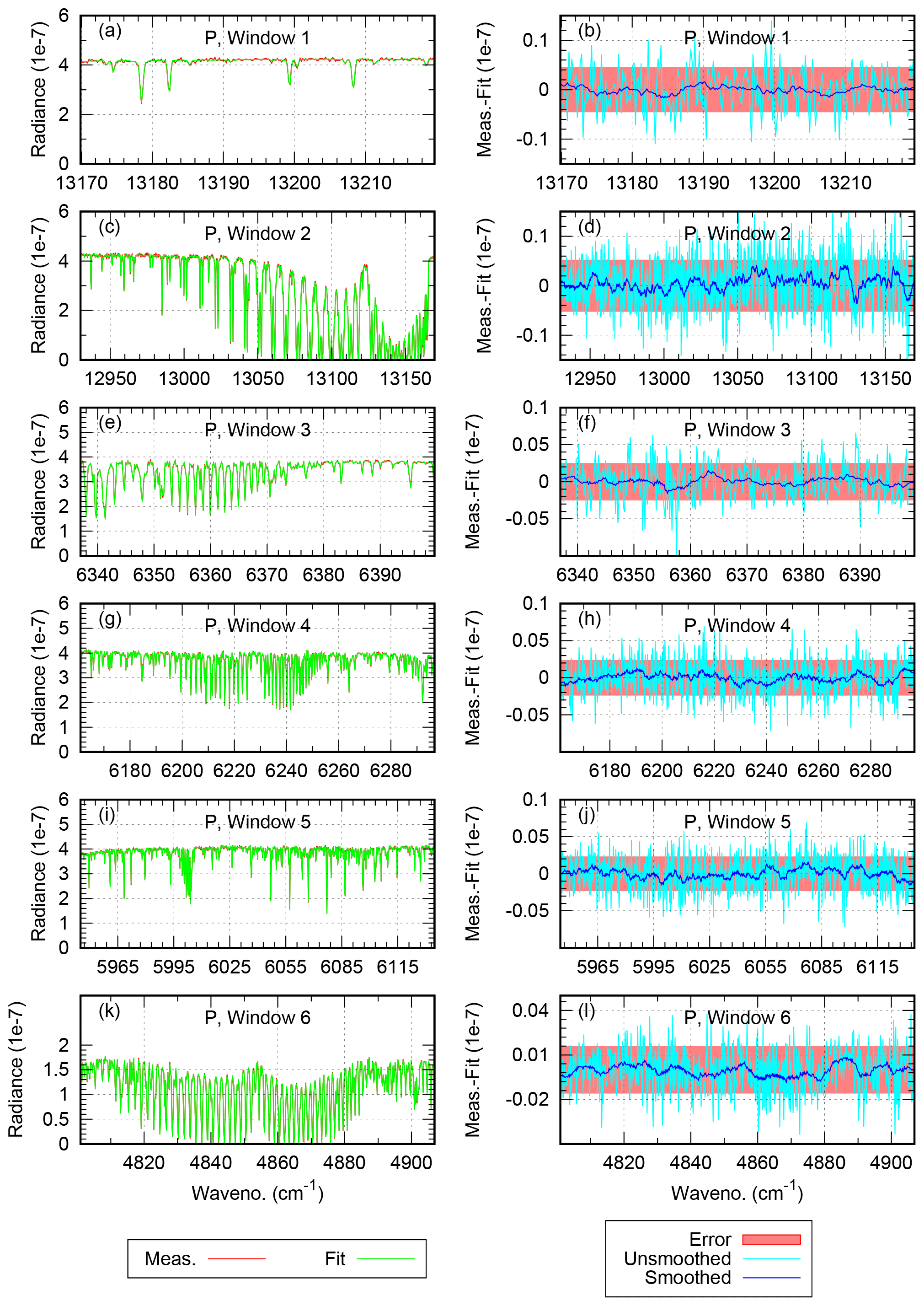
Figure 8Example for a single GOSAT measurement (P polarisation): (a, c, e, g, i, k) measured (red) and retrieved (green) spectra in the different fit windows; because of the good agreement the red curve is essentially barely visible below the green curve. (b, d, f, h, j, l) Corresponding residuals (measurement – fit). Light blue: unsmoothed. Blue: smoothed with a boxcar width of 21 spectral pixels (=4.2 cm−1). Red: estimated noise error range. The radiance unit is W cm−2 cm sr−1.
In Fig. 10 some statistical information about the GOSAT-FOCAL data products is given. A time series for the number of valid data is given in the top plot. In recent years, about 5 %–6 % of the available measurements could be transferred to valid XCO2 data. The number of valid data points increases from 2009 to 2019. This is mainly due to an increase in the data over water, which is related to optimisations in GOSAT operations (better use of glint geometry) over water. As expected, the mean global XCO2 shown in the middle plot increases with time. Global mean values over water are typically slightly higher than over land. The observed XCO2 variability (standard deviation, bottom plot) is larger over land. Part of this variability is attributed to influences of surface elevation and to different scattering pathways between the land and water measurements. For GOSAT-2, only retrieved data from 2019 are available so far. The total number of available measurements is about 2.8 million compared to about 3.5 million GOSAT measurements in 2019. Only about 3 % of the GOSAT-2 data remain after all filtering and post-processing, which is roughly half of the corresponding number for GOSAT (but similar to the first year of GOSAT). As can be seen from Fig. 3 more GOSAT-2 data are filtered out due to failed or bad convergence and by the RSR outlier limits than for GOSAT (Fig. 2). Future improvements of the GOSAT-2 calibration or the noise model are considered to help here.
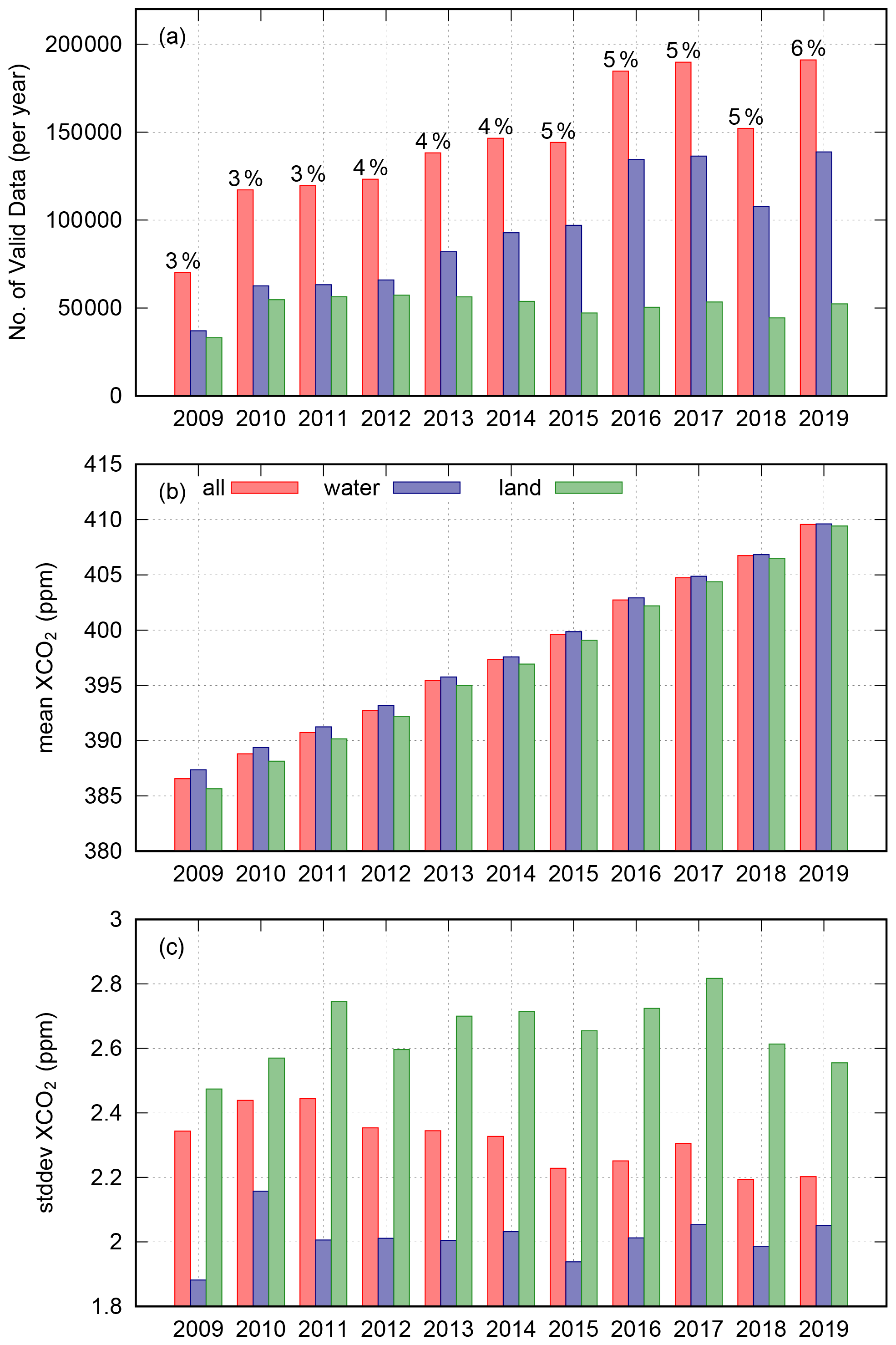
Figure 10Statistics for valid GOSAT measurements (after pre- and post-processing filtering) for each year. Blue: measurements over water. Green: measurements over land. Red: all data. (a) Number of valid measurements, including the percentage of all originally available measurements. (b) Global mean XCO2. (c) Corresponding standard deviation.
For further analyses, we have generated monthly maps on a grid. Example plots for the months April and August 2019 (the beginning and end of the growing season) are shown in Fig. 11 for GOSAT and in Fig. 12 for GOSAT-2. The data are not filtered for low numbers of input data in the grid points, which explains some individual outliers in the plots. Overall, the spatial patterns observed by GOSAT and GOSAT-2 look reasonable. The north–south gradient in XCO2 is visible with a different sign in April and August for both instruments. The spatial coverage of the GOSAT-2 data is lower than for GOSAT because more data are filtered out (see above). This especially affects regions like the northern part of Africa.

Figure 11Example for gridded GOSAT XCO2 data. (a) April 2019. (b) August 2019.
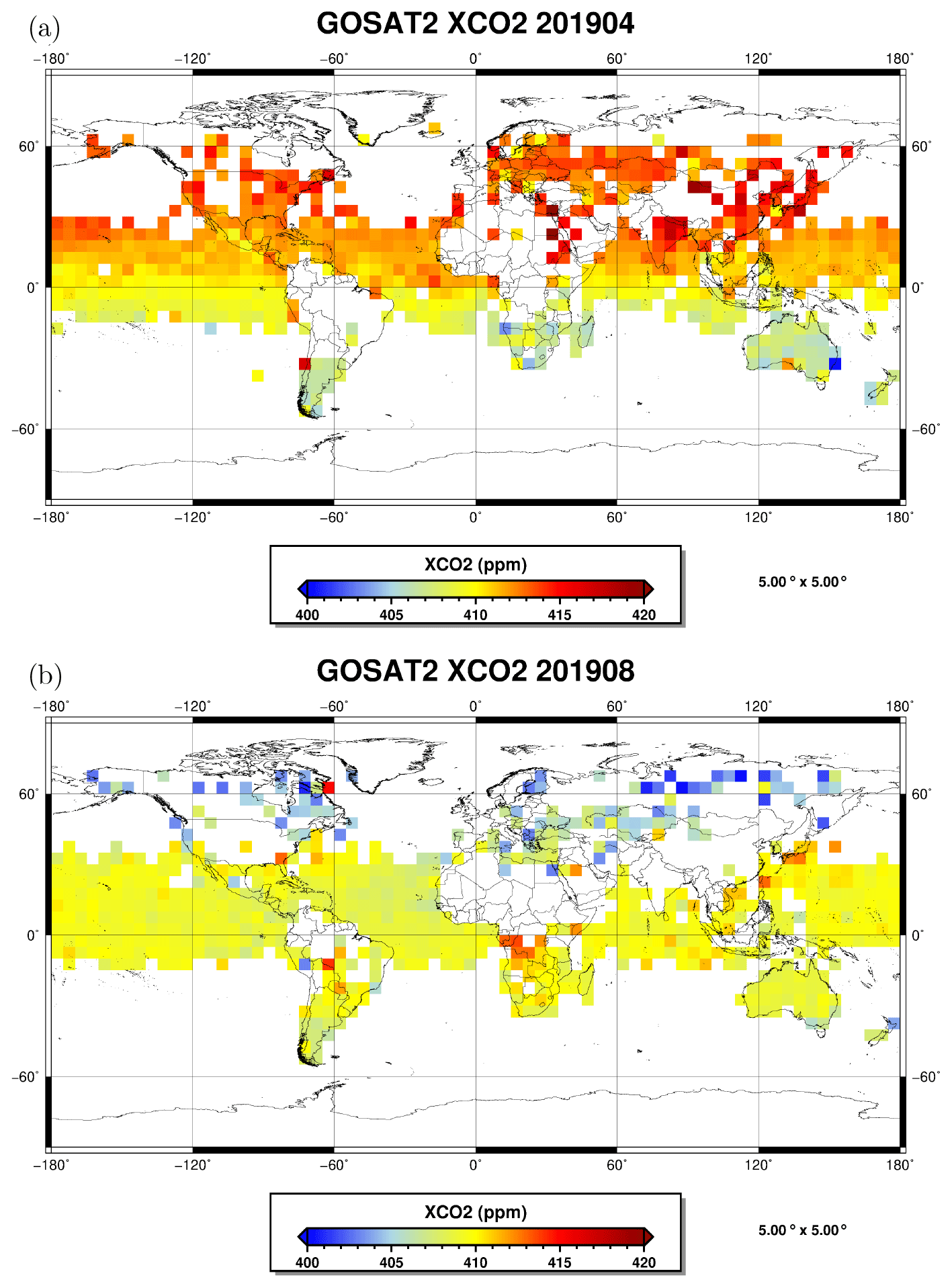
Figure 12Example for gridded GOSAT-2 XCO2 data. (a) April 2019. (b) August 2019.
For the verification and validation of the GOSAT- and GOSAT-2-FOCAL products we perform a comparison with various reference data sets (see Sect. 2), namely the following.
-
The GOSAT BESD v01.04 product from IUP (referred to as BESD later).
-
The GOSAT ACOS v9r product from NASA (referred to as ACOS later).
-
The GOSAT UoL_FP v7.3 product from the University of Leicester (referred to as UoL later).
-
The GOSAT RemoTeC v2.3.8 product from SRON (referred to as SRON later).
-
The GOSAT operational product v02.95 (bias corrected) from NIES (referred to as NIES later).
-
Collocated TCCON GGG2014 data (referred to as TCCON later).
For the comparisons, all data have been adjusted using the same a priori (SECM2020).
Since all GOSAT products use different retrieval and filter methods, they do not contain the same number of data (see Fig. 13). Currently, the NASA ACOS product has the largest number of valid data points, followed by the new GOSAT-FOCAL product with about 20 % less data.
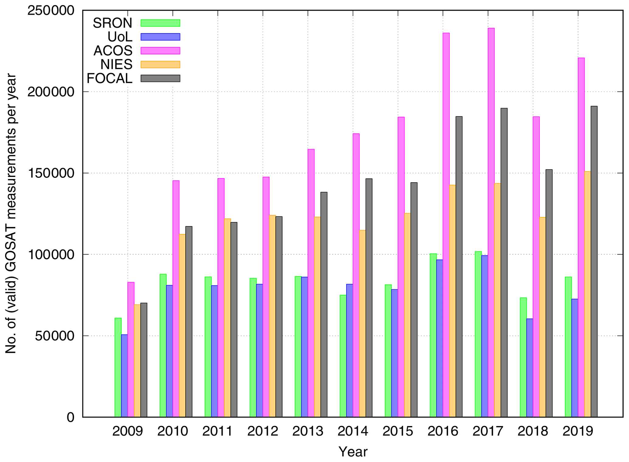
Figure 13Number of valid XCO2 data points in the different GOSAT products from 2009 to 2019.
5.1 Direct comparisons
There are enough common measurement points included in the different GOSAT products to perform a direct comparison. Figure 14 shows as an example a comparison between the GOSAT-FOCAL data for the year 2018 with the corresponding ACOS, BESD, SRON, NIES, and UoL products. For each plot we only use data for which both data sets have a valid XCO2 value. For these data we performed a linear regression using the orthogonal distance regression (ODR) method (see e.g. Boggs et al., 1987). Unlike common linear regression, ODR considers uncertainties for both axes (data sets) by minimising the orthogonal distances between the model curve and the data points. The ODR results are shown by the red line and its label. The number of collocations, the median and mean, and the standard deviations of the differences are given in the titles.

Figure 14Comparison of GOSAT-FOCAL data (x axis) from 2018 with other GOSAT data (y axis). The colour of the data points corresponds to the density of data points at that location (normalised to a maximum value of 1). The dashed line corresponds to perfect agreement. The red line shows the result of a linear fit using the orthogonal distance regression (ODR) method. The total number of collocated data as well as the median, mean, and standard deviation of the XCO2 differences between the two data sets are given in the title of the sub-plots. (a) FOCAL vs. ACOS. (b) FOCAL vs. BESD. (c) FOCAL vs. NIES. (d) FOCAL vs. SRON. (e) FOCAL vs. UoL.
Overall, the data scatter around the 1:1 line in a similar way for all comparisons. ODR slopes vary between the data sets from 0.84 (for FOCAL vs. ACOS) up to 1.08 (for FOCAL vs. BESD). Most collocations are available for the ACOS data set because this has the largest number of valid data. Mean and median differences are quite similar and reach from −0.17 ppm (comparison to BESD) to 0.67 ppm (comparison with UoL). The scatter (standard deviation of the differences) reaches from 1.4 ppm (ACOS, NIES) to 1.8 ppm (BESD).
5.2 TCCON comparisons
TCCON provides high-quality XCO2 (and other) data, which are currently considered to be the main reference for greenhouse gas data obtained from satellite measurements. Therefore, we compared the different GOSAT data sets with collocated TCCON measurements from 2009 to the end of 2018. BESD data are not included because they do not cover the complete time interval. Collocation criteria are the following:
-
maximum time difference of 2 h;
-
maximum spatial distance of satellite measurement from TCCON station of 500 km; and
-
maximum surface elevation difference between satellite measurement and TCCON station of 250 m.
In addition to these criteria we also consider in the validation only stations and TCCON data sets which have at least 50 collocations for all algorithms. This improves the comparability of regional and seasonal biases. As a consequence, not all stations listed in Table 1 contribute to the validation.
The comparison procedure is the same as used by Reuter et al. (2020) and described by Reuter et al. (2019b). In summary, for each TCCON site, the time series of satellite minus TCCON differences are computed under consideration of the averaging kernels, i.e. different vertical sensitivities. The resulting time series are fitted with a trend model, which includes an offset term, a slope term, and a sine term for seasonal fluctuations. The offset term is considered the station bias, and the station scatter is computed from the standard deviation of the fit residual. Results for the GOSAT time series at the TCCON stations are shown in Fig. 15. Overall, the temporal variations of XCO2 are well reproduced by all data.
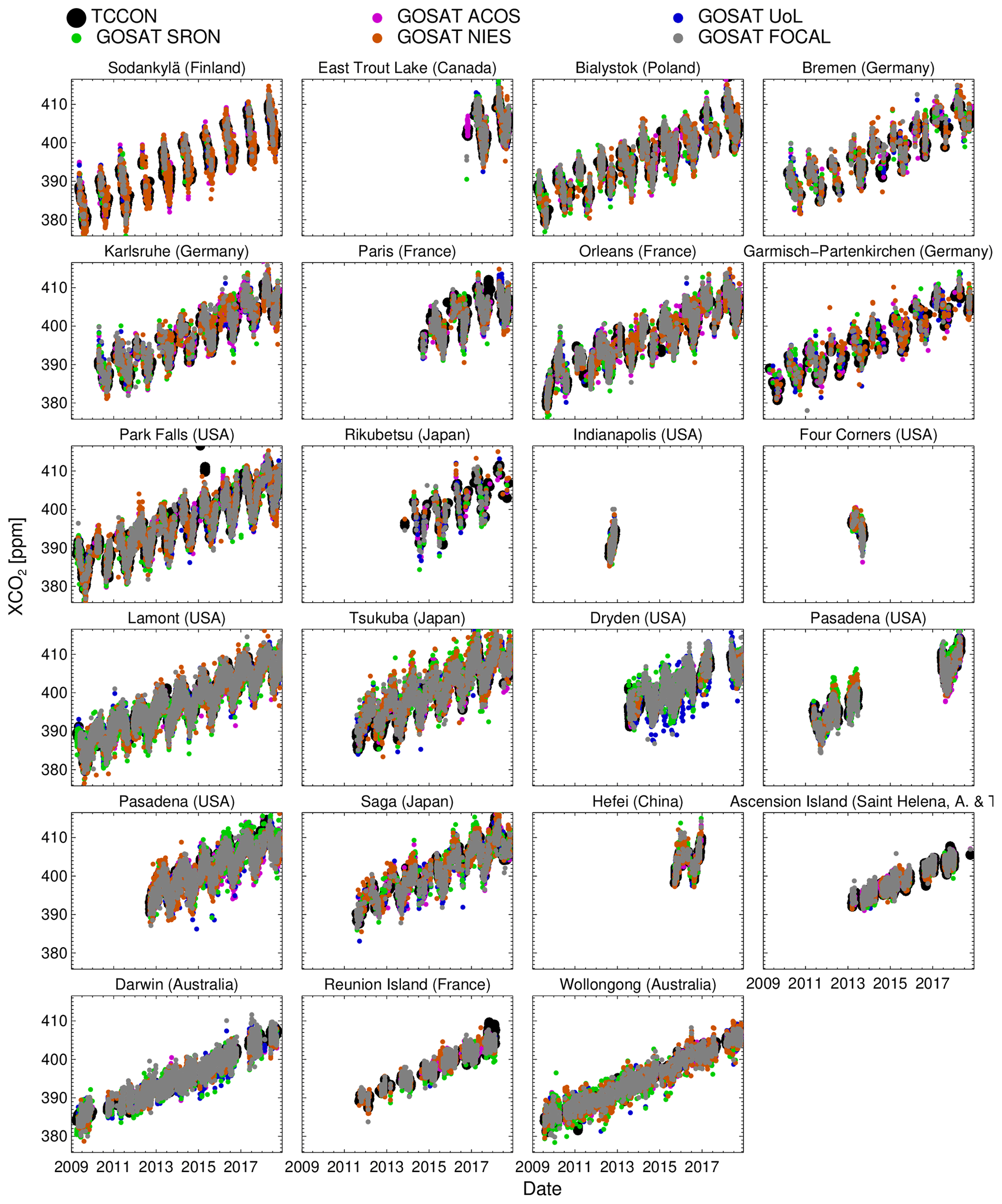
Figure 15Time series of collocated GOSAT data at various TCCON sites for different data products including the new GOSAT-FOCAL data set.
Figure 16 shows as a summary of the GOSAT TCCON comparisons the derived bias and scatter for the different stations and products. The new GOSAT-FOCAL product compares well with the other data sets. Its differences to TCCON have a station-to-station bias (the standard deviation of the station bias) of 0.56 ppm and a mean scatter (root mean square, or rms, scatter per station) of 1.89 ppm. The seasonal component of the bias has a station-to-station average standard deviation of 0.37 ppm. Overall, the ACOS product performs best in this comparison.
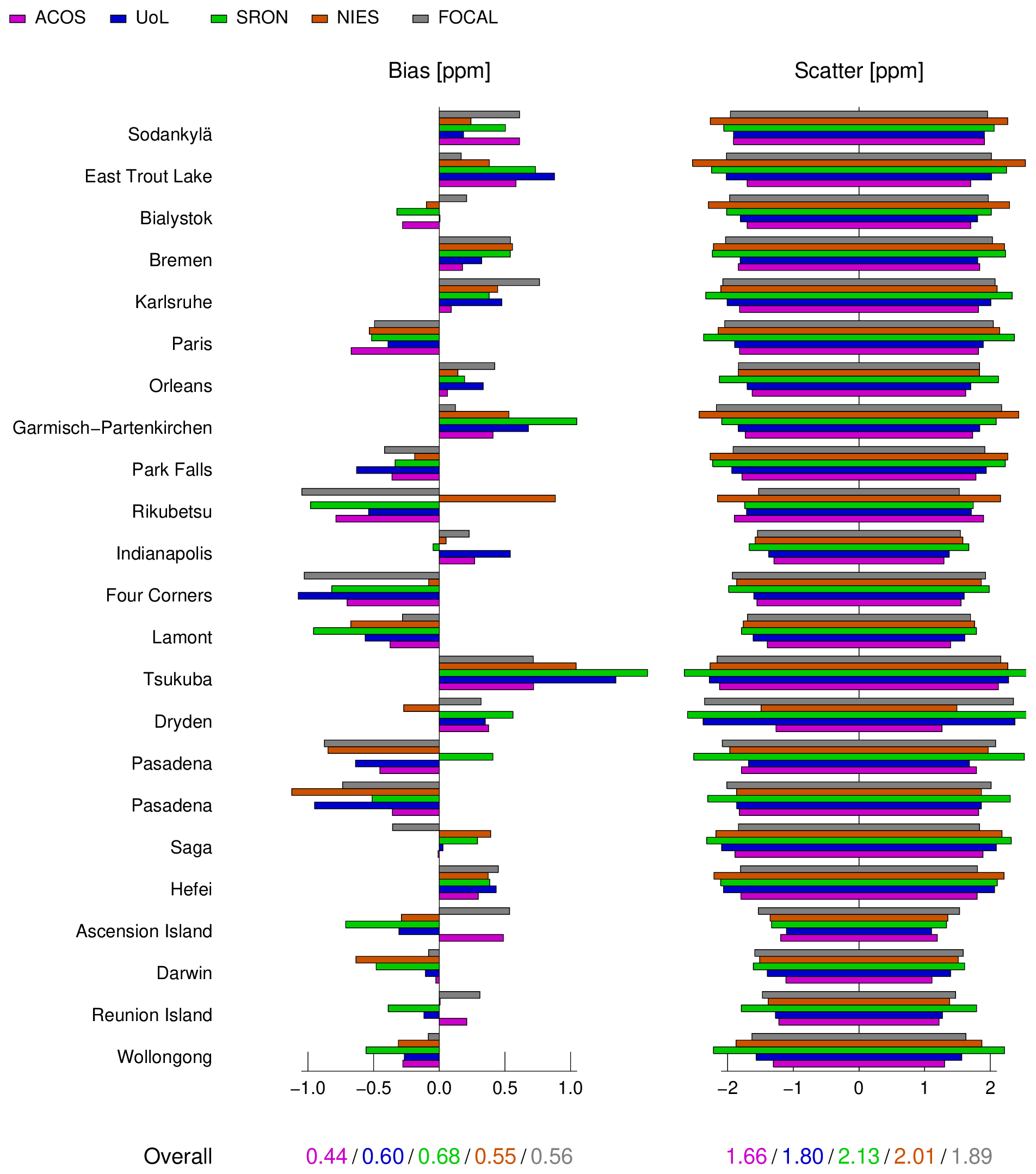
Note that the biases shown in Fig. 16 essentially correspond to a bias anomaly since the mean bias over all stations was removed from all products. This is because for most applications this mean bias is not relevant since most information is contained in gradients. Subtracting a mean bias also facilitates a comparison of different bias patterns between the algorithms. The subtracted mean station bias is actually small; for GOSAT it varies between 0.17 ppm (for ACOS) and 0.64 ppm (for NIES). Because of the subtracted mean bias different signs of biases for different products could be coincidental. However, the biases of FOCAL and ACOS are consistent with the biases found by Reuter et al. (2020).
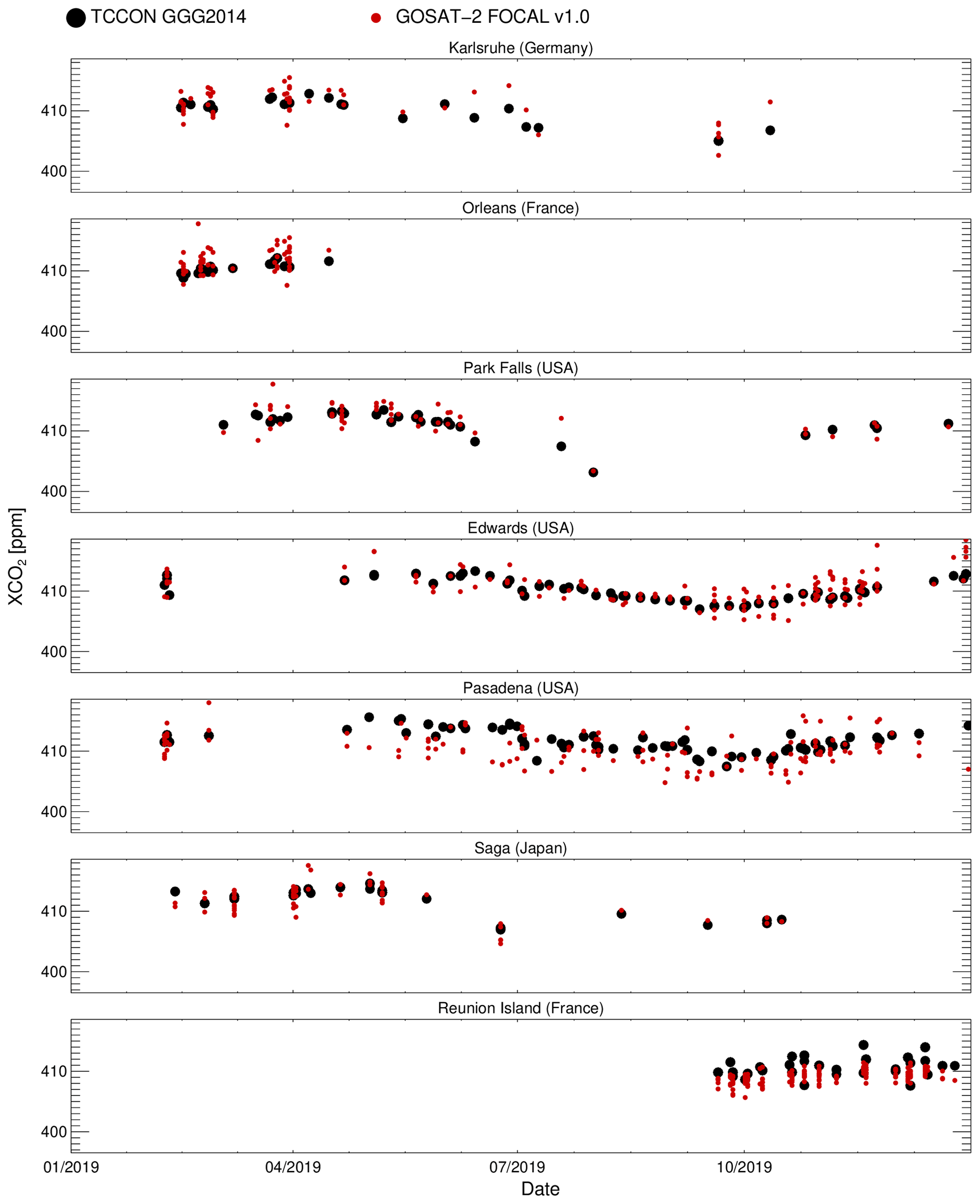
In Figs. 17 and 18 we show results from a preliminary comparison of the new GOSAT-2-FOCAL data with TCCON. These results are considered less reliable because they are based on a data set which covers less than a year. There are sufficient collocations for only seven TCCON stations, and some of them comprise only a few months of data, which limits the fit of our trend model. The mean scatter of the GOSAT-2 data is 1.86 ppm and therefore similar to the one for GOSAT. The derived station-to-station bias for GOSAT-2-FOCAL is 1.14 ppm. This high value is mainly due to the biases derived for the stations Orleans and Réunion Island (where few data are available) as well as the station Pasadena, which also showed larger discrepancies to the GOSAT products (see Fig. 16). We are confident that the station-to-station bias will improve when more and improved GOSAT-2 data are available.

Via the TCCON comparison it is also possible to validate the reported precision of the FOCAL data products (i.e. the specified XCO2 error). The basic idea is to estimate the true precision from the variability of the XCO2 bias relative to trend-corrected, collocated TCCON data. For this purpose, we define 20 bins with increasing reported XCO2 uncertainty and compute the corresponding true precision from the scatter relative to TCCON (i.e. the fit residual mentioned above).
The corresponding scatter plot is shown in Fig. 19. We use the fitted linear curve to correct the reported uncertainty of the GOSAT-FOCAL data. After the correction, all data scatter around the 1:1 line (dashed).
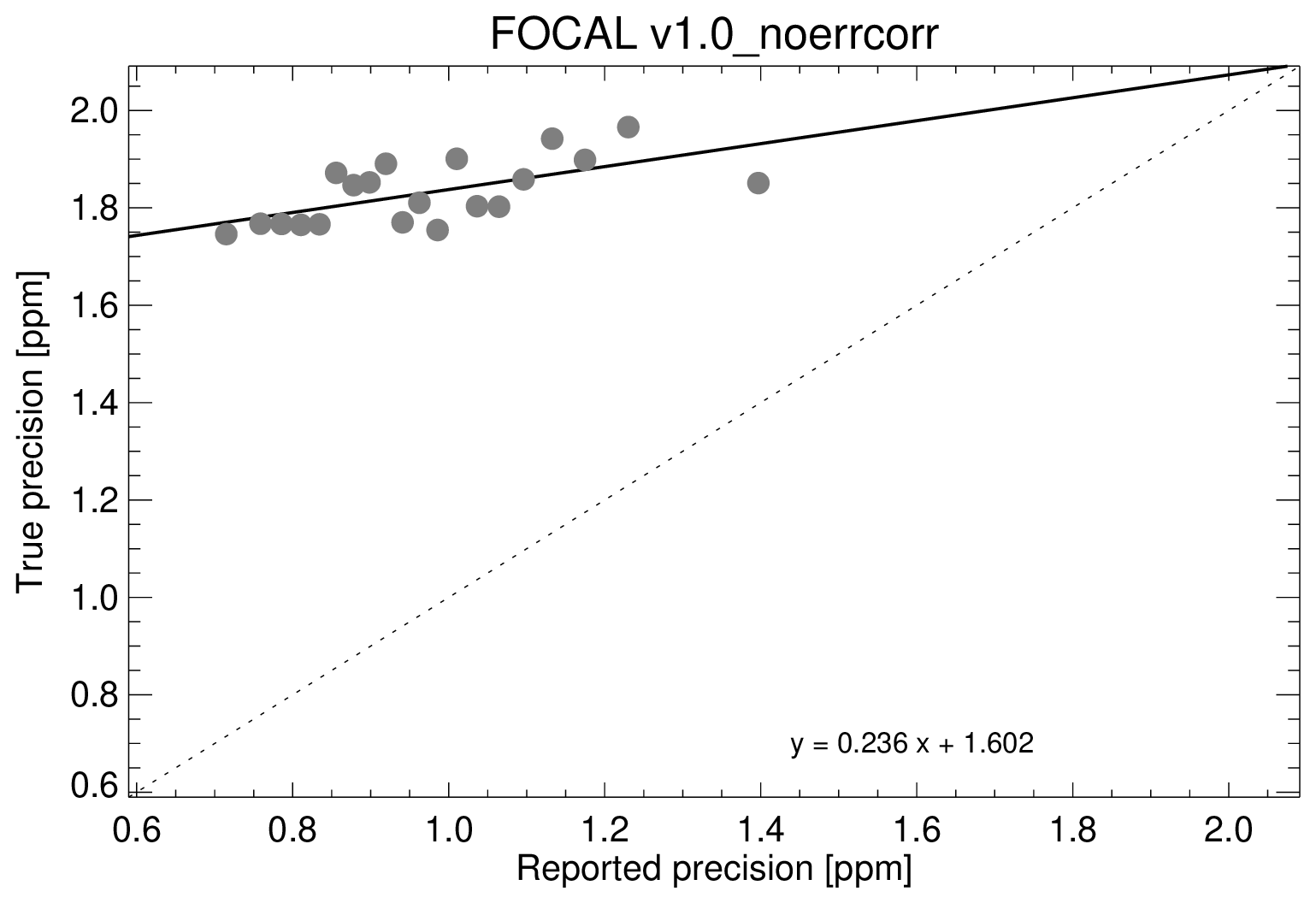
Figure 19Comparisons of the (binned) original XCO2 errors (reported precision without correction) of the GOSAT-FOCAL product with estimated errors based on collocated TCCON data (true precision).
A similar correction will be performed for the GOSAT-2-FOCAL product as soon as sufficient data (GOSAT-2 and TCCON) are available, which is currently not the case.
5.3 Time series
To investigate the temporal behaviour of the FOCAL XCO2 data sets, we performed comparisons based on monthly data from 2009 to 2019, which were spatially gridded to (examples are shown in Figs. 11 and 12). Similar data sets have been generated for the SRON, UoL, ACOS, and NIES GOSAT products. We also produced a corresponding gridded GOSAT BESD data set; since these are near-real-time (NRT) data only, there are no GOSAT BESD data before 2014 available (when the NRT processing started). GOSAT-2 data start in February 2019.
We then selected grid points for which the standard error of the mean is less than 1.6 ppm for each combination of GOSAT-FOCAL XCO2 and a correlative data set (as a basic quality filter, similar as done by Reuter et al., 2020). These data were then averaged over different latitudinal ranges, namely
-
global (90∘ S–90∘ N),
-
the Northern Hemisphere (25–90∘ N),
-
the tropics (25∘ S–25∘ N), and
-
the Southern Hemisphere (25–90∘ S).
Figure 20 shows the results of these comparisons. The left plots display time series of the different data sets and the right plots the difference between the GOSAT-FOCAL XCO2 and the reference data. All data products reproduce the overall increase in XCO2 with time and the seasonal variations. On average, FOCAL data are typically about 0.5 ppm higher than the other data sets (except for BESD). This is related to the choice of the true XCO2 for the bias correction. There are long-term changes of the order of 1 ppm over the complete time series, which differ for each data set. For example, the GOSAT-FOCAL data show in the tropics relative to SRON a higher value at the start of the time series, but both data sets agree at the end. On the other hand, the average difference to the UoL data in the Northern Hemisphere is negative during the first years, but it increases to an almost constant small positive offset below about 0.5 ppm. There is not much difference in the temporal behaviour between the GOSAT-FOCAL and the ACOS and NIES time series. The seasonal shapes also differ slightly, with amplitudes of about 0.5 ppm and somewhat larger differences in the Southern Hemisphere where seasonal variations are generally smaller.
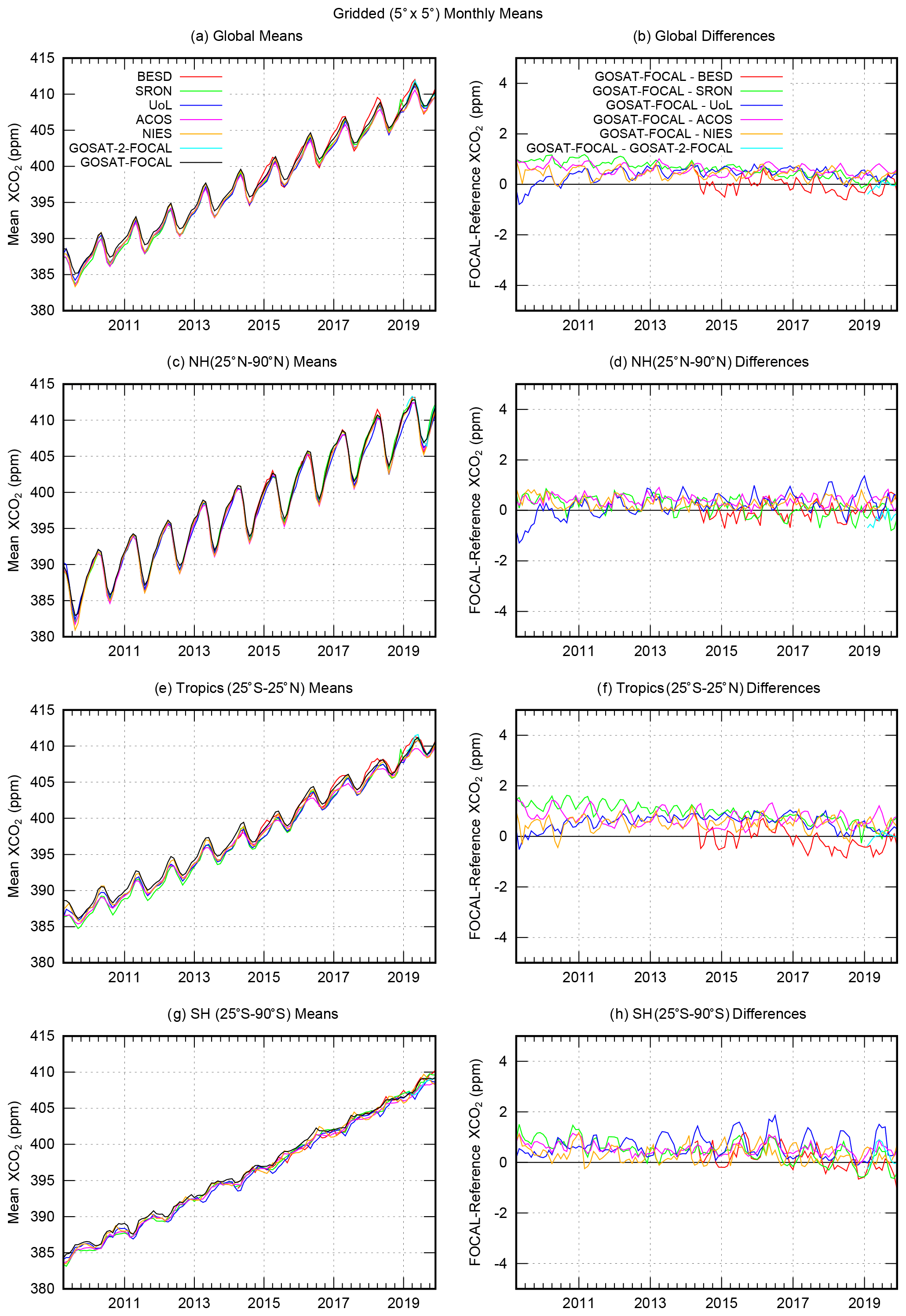
Figure 20Gridded monthly mean time series of different GOSAT XCO2 products. (a, c, e, g) Time series of mean XCO2 for four different regions (from top to bottom: global, Northern Hemisphere, tropics, Southern Hemisphere). (b, d, f, h) Corresponding differences to the GOSAT-FOCAL product.
Overall, the agreement within the GOSAT data sets is broadly consistent with the systematic regional and seasonal biases derived from the TCCON validation, especially considering that all gridded data sets are based on a different spatial and temporal sampling. Also, the FOCAL products for GOSAT and GOSAT-2 seem to agree quite well, but more GOSAT-2 data are needed to confirm this.
Based on the FOCAL retrieval method a new XCO2 data set for GOSAT and a first XCO2 data set for GOSAT-2 have been generated, making use of both measured polarisation directions. The GOSAT-FOCAL data set compares well with corresponding data from other currently available GOSAT retrieval algorithms, i.e. the RemoTeC product from SRON, the UoL FP product, the NASA ACOS product, the NIES product, and the BESD product from IUP. All data sets use different filtering and bias correction schemes and therefore also comprise a different number and sampling of data. The GOSAT-FOCAL product performs well in this context and has almost as many valid data as the ACOS product. Based on gridded data, differences in long-term variations of all data sets of the order of 1 ppm per decade are observed. Also, seasonal variations differ by about 0.5 ppm.
Comparisons with ground-based TCCON data reveal for the GOSAT-FOCAL product an overall station-to-station bias of 0.56 ppm and a mean scatter of 1.89 ppm. These values are comparable to and in some cases even better than those of the already existing GOSAT products, some of which have less valid data.
The first GOSAT-2 results using the FOCAL method are also quite promising, but further investigations, longer time series, and more correlative data sets are required for a quantitative assessment of the GOSAT-2-FOCAL data quality.
Overall, the FOCAL method has proven to be computationally fast and to produce XCO2 results with similar accuracy as other, typically more time-consuming, retrieval algorithms. This is the case not only when applied to OCO-2 but also for GOSAT and GOSAT-2. FOCAL is therefore considered to be a good candidate algorithm for future satellite sensors producing large amounts of data, like the forthcoming European anthropogenic CO2 Monitoring (CO2M) mission.
The GOSAT-FOCAL V1.0 data set and the preliminary GOSAT-2-FOCAL data are available on request from the authors.
SN adapted the FOCAL method to GOSAT and GOSAT-2, generated the FOCAL data products, and performed the validation. MR developed the FOCAL method and provided the XCO2 reference databases and the TCCON validation tools. JB provided the Python implementation used for the SC4C methane climatology from Schneising et al. (2019). MH provided the original Python implementation of FOCAL (OCO-2 version). ADN and YY provided the UoL and NIES GOSAT data products. HS provided information on GOSAT and GOSAT-2, especially the preliminary GOSAT-2 ILS.
The following co-authors provided TCCON data: MB, NMD, DGF, DWTG, FH, RK, IM, JN, HO, CP, JRP, DFP, MKS, KS, RS, YT, VAV, and TW.
All authors provided support in writing the paper.
The authors declare that they have no conflict of interest.
GOSAT and GOSAT-2 spectral data have been provided by JAXA and NIES. CarbonTracker CT2019 and CT-NRT.v2020-1 results were provided by NOAA ESRL (Boulder, Colorado, USA) from the website at http://carbontracker.noaa.gov (last access: 8 May 2021). ABSCO cross sections for CO2 were provided by NASA and the ACOS/OCO-2 team. GMTED2010 topography data were provided by the US Geological Survey (USGS) and the National Geospatial-Intelligence Agency (NGA). We thank the European Centre for Medium-Range Weather Forecasts (ECMWF) for providing us with analysed meteorological fields (ERA5 data).
We thank the OCO-2 Science Team for the GOSAT ACOS Level 2 XCO2 product obtained from https://oco2.gesdisc.eosdis.nasa.gov/data/GOSAT_TANSO_Level2/ACOS_L2_Lite_FP.9r/ (https://doi.org/10.5067/VWSABTO7ZII4; last access: 16 October 2020). The SRON GOSAT XCO2 data product has been obtained from the Copernicus Climate Data Store (https://cds.climate.copernicus.eu/, last assess: 15 October 2020).
We used TCCON GGG2014 ground-based validation data (see Table 1). TCCON data from the Eureka and Izaña stations were provided by Kimberly Strong and Omaira E. Garcia, respectively. The Ascension Island TCCON station has been supported by the European Space Agency (ESA) under grant 4000120088/17/I-EF and by the German Bundesministerium für Wirtschaft und Energie (BMWi) under grants 50EE1711C and 50EE1711E. We thank the ESA Ariane tracking station at North East Bay, Ascension Island, for hosting and local support. The TCCON site at Réunion Island has been operated by the Royal Belgian Institute for Space Aeronomy with financial support since 2014 by the EU project ICOS-Inwire and the ministerial decree for ICOS (FR/35/IC1 to FR/35/C5), with local activities supported by LACy/UMR8105 – Université de La Réunion. The Paris TCCON site has received funding from Sorbonne Université, the French research centre CNRS, the French space agency CNES, and Région Île-de-France. The TCCON stations at Rikubetsu, Tsukuba, and Burgos are supported in part by the GOSAT series project. Local support for Burgos is provided by the Energy Development Corporation (EDC, Philippines). Nicholas M. Deutscher is funded by ARC Future Fellowship FT180100327. The Darwin and Wollongong TCCON stations are supported by ARC grants DP160100598, LE0668470, DP140101552, DP110103118, and DP0879468; Darwin receives additional support from NASA grants NAG5-12247 and NNG05-GD07G as well as technical assistance from the Australian Bureau of Meteorology. The TCCON stations Garmisch and Zugspitze have been supported by the European Space Agency (ESA) under grant 4000120088/17/I-EF and by the German Bundesministerium für Wirtschaft und Energie (BMWi) via the DLR under grant 50EE1711D as well as by the Helmholtz Society via the research programme ATMO.
This work has received funding from JAXA (GOSAT and GOSAT-2 support, contracts 19RT000692 and JX-PSPC-527269), EUMETSAT (FOCAL-CO2M study, contract EUM/CO/19/4600002372/RL), the ESA (GHG-CCI+ project, contract 4000126450/19/I-NB), and the State and the University of Bremen.
The article processing charges for this open-access publication were covered by the University of Bremen.
This paper was edited by Joanna Joiner and reviewed by two anonymous referees.
Anderson, G., Clough, S., Kneizys, F., Chetwynd, J., and Shettle, E.: AFGL Atmospheric Constituent Profiles (0–120km), Environmental Research Papers No. 954, AFGL-TR-86-0110, https://www.researchgate.net/publication/235054307_AFGL_Atmospheric_Constituent_Profiles_0120km (last access: 7 August 2020), 1986. a
Basu, S., Guerlet, S., Butz, A., Houweling, S., Hasekamp, O., Aben, I., Krummel, P., Steele, P., Langenfelds, R., Torn, M., Biraud, S., Stephens, B., Andrews, A., and Worthy, D.: Global CO2 fluxes estimated from GOSAT retrievals of total column CO2, Atmos. Chem. Phys., 13, 8695–8717, https://doi.org/10.5194/acp-13-8695-2013, 2013. a
Benner, D. C., Devi, V. M., Sung, K., Brown, L. R., Miller, C. E., Payne, V. H., Drouin, B. J., Yu, S., Crawford, T. J., Mantz, A. W., Smith, M. A. H., and Gamache, R. R.: Line parameters including temperature dependences of air- and self-broadened line shapes of 12C16O2: 2.06-µm region, J. Mol. Spectrosc., 326, 21–47, https://doi.org/10.1016/j.jms.2016.02.012, 2016. a
Blumenstock, T., Hase, F., Schneider, M., García, O. E., and Sepúlveda, E.: TCCON data from Izana (ES), Release GGG2014.R1, CaltechDATA [data set], https://doi.org/10.14291/TCCON.GGG2014.IZANA01.R1, 2017. a
Boggs, P. T., Byrd, R. H., and Schnabel, R. B.: A Stable and Efficient Algorithm for Nonlinear Orthogonal Distance Regression, SIAM J. Sci. Stat. Comput., 8, 1052–1078, https://doi.org/10.1137/0908085, 1987. a
Bovensmann, H., Burrows, J. P., Buchwitz, M., Frerick, J., Noël, S., Rozanov, V. V., Chance, K. V., and Goede, A. H. P.: SCIAMACHY – Mission Objectives and Measurement Modes, J. Atmos. Sci., 56, 127–150, 1999. a, b
Buchwitz, M., Reuter, M., Schneising, O., Noël, S., Gier, B., Bovensmann, H., Burrows, J. P., Boesch, H., Anand, J., Parker, R. J., Somkuti, P., Detmers, R. G., Hasekamp, O. P., Aben, I., Butz, A., Kuze, A., Suto, H., Yoshida, Y., Crisp, D., and O'Dell, C.: Computation and analysis of atmospheric carbon dioxide annual mean growth rates from satellite observations during 2003–2016, Atmos. Chem. Phys., 18, 17355–17370, https://doi.org/10.5194/acp-18-17355-2018, 2018. a
Burrows, J., Hölzle, E., Goede, A., Visser, H., and Fricke, W.: SCIAMACHY – scanning imaging absorption spectrometer for atmospheric chartography, Acta Astronaut., 35, 445–451, https://doi.org/10.1016/0094-5765(94)00278-T, 1995. a
Butz, A., Guerlet, S., Hasekamp, O., Schepers, D., Galli, A., Aben, I., Frankenberg, C., Hartmann, J.-M., Tran, H., Kuze, A., Keppel-Aleks, G., Toon, G., Wunch, D., Wennberg, P., Deutscher, N., Griffith, D., Macatangay, R., Messerschmidt, J., Notholt, J., and Warneke, T.: Toward accurate CO2 and CH4 observations from GOSAT, Geophys. Res. Lett., 38, L14812, https://doi.org/10.1029/2011GL047888, 2011. a, b
Chevallier, F.: On the statistical optimality of CO2 atmospheric inversions assimilating CO2 column retrievals, Atmos. Chem. Phys., 15, 11133–11145, https://doi.org/10.5194/acp-15-11133-2015, 2015. a
Chevallier, F., Palmer, P. I., Feng, L., Boesch, H., O'Dell, C. W., and Bousquet, P.: Towards robust and consistent regional CO2 flux estimates from in situ and space-borne measurements of atmospheric CO2, Geophys. Res. Lett., 41, 1065–1070, https://doi.org/10.1002/2013GL058772, 2014. a
Ciais, P., Dolman, A. J., Bombelli, A., Duren, R., Peregon, A., Rayner, P. J., Miller, C., Gobron, N., Kinderman, G., Marland, G., Gruber, N., Chevallier, F., Andres, R. J., Balsamo, G., Bopp, L., Bréon, F.-M., Broquet, G., Dargaville, R., Battin, T. J., Borges, A., Bovensmann, H., Buchwitz, M., Butler, J., Canadell, J. G., Cook, R. B., DeFries, R., Engelen, R., Gurney, K. R., Heinze, C., Heimann, M., Held, A., Henry, M., Law, B., Luyssaert, S., Miller, J., Moriyama, T., Moulin, C., Myneni, R. B., Nussli, C., Obersteiner, M., Ojima, D., Pan, Y., Paris, J.-D., Piao, S. L., Poulter, B., Plummer, S., Quegan, S., Raymond, P., Reichstein, M., Rivier, L., Sabine, C., Schimel, D., Tarasova, O., Valentini, R., Wang, R., van der Werf, G., Wickland, D., Williams, M., and Zehner, C.: Current systematic carbon-cycle observations and the need for implementing a policy-relevant carbon observing system, Biogeosciences, 11, 3547–3602, https://doi.org/10.5194/bg-11-3547-2014, 2014. a
Cogan, A. J., Boesch, H., Parker, R. J., Feng, L., Palmer, P. I., Blavier, J.-F. L., Deutscher, N. M., Macatangay, R., Notholt, J., Roehl, C., Warneke, T., and Wunch, D.: Atmospheric carbon dioxide retrieved from the Greenhouse gases Observing SATellite (GOSAT): Comparison with ground-based TCCON observations and GEOS-Chem model calculations, J. Geophys. Res., 117, D21301, https://doi.org/10.1029/2012JD018087, 2012. a, b, c
Crisp, D., Atlas, R. M., Bréon, F.-M., Brown, L. R., Burrows, J. P., Ciais, P., Connor, B. J., Doney, S. C., Fung, I. Y., Jacob, D. J., Miller, C. E., O'Brien, D., Pawson, S., Randerson, J. T., Rayner, P., Salawitch, R. S., Sander, S. P., Sen, B., Stephens, G. L., Tans, P. P., Toon, G. C., Wennberg, P. O., Wofsy, S. C., Yung, Y. L., Kuang, Z., Chudasama, B., Sprague, G., Weiss, P., Pollock, R., Kenyon, D., and Schroll, S.: The Orbiting Carbon Observatory (OCO) mission, Adv. Space Res., 34, 700–709, 2004. a
Crisp, D., Pollock, H. R., Rosenberg, R., Chapsky, L., Lee, R. A. M., Oyafuso, F. A., Frankenberg, C., O'Dell, C. W., Bruegge, C. J., Doran, G. B., Eldering, A., Fisher, B. M., Fu, D., Gunson, M. R., Mandrake, L., Osterman, G. B., Schwandner, F. M., Sun, K., Taylor, T. E., Wennberg, P. O., and Wunch, D.: The on-orbit performance of the Orbiting Carbon Observatory-2 (OCO-2) instrument and its radiometrically calibrated products, Atmos. Meas. Tech., 10, 59–81, https://doi.org/10.5194/amt-10-59-2017, 2017. a
Danielson, J. and Gesch, D.: Global multi-resolution terrain elevation data 2010 (GMTED2010), Open-File Report 2011-1073, Tech. rep., U.S. Geological Survey, https://doi.org/10.3133/ofr20111073, 2011 a
Davis, S. P., Abrams, M. C., and Brault, J. W. (Eds.): 5 – Nonideal (real-world) interferograms, in: Fourier Transform Spectrometry, Academic Press, San Diego, 67–80, https://doi.org/10.1016/B978-012042510-5/50005-6, 2001. a
De Mazière, M., Sha, M. K., Desmet, F., Hermans, C., Scolas, F., Kumps, N., Metzger, J.-M., Duflot, V., and Cammas, J.-P.: TCCON data from Réunion Island (RE), Release GGG2014.R1 (Version R1), CaltechDATA [data set], https://doi.org/10.14291/TCCON.GGG2014.REUNION01.R1, 2017. a
Deutscher, N. M., Notholt, J., Messerschmidt, J., Weinzierl, C., Warneke, T., Petri, C., and Grupe, P.: TCCON data from Bialystok (PL), Release GGG2014.R2 (Version R2), CaltechDATA [data set], https://doi.org/10.14291/TCCON.GGG2014.BIALYSTOK01.R2, 2019. a
Devi, V. M., Benner, D. C., Sung, K., Brown, L. R., Crawford, T. J., Miller, C. E., Drouin, B. J., Payne, V. H., Yu, S., Smith, M. A. H., Mantz, A. W., and Gamache, R. R.: Line parameters including temperature dependences of self- and air-broadened line shapes of 12C16O2: 1.6-µm region, J. Quant. Spectrosc. Ra., 177, 117–144, https://doi.org/10.1016/j.jqsrt.2015.12.020, 2016. a
Dubey, M., Lindenmaier, R., Henderson, B., Green, D., Allen, N., Roehl, C., Blavier, J.-F., Butterfield, Z., Love, S., Hamelmann, J., and Wunch, D.: TCCON data from Four Corners (US), Release GGG2014R0 (Version GGG2014.R0), TCCON data archive, CaltechDATA [data set], https://doi.org/10.14291/tccon.ggg2014.fourcorners01.R0/1149272, 2014. a
Eldering, A., Wennberg, P. O., Crisp, D., Schimel, D. S., Gunson, M. R., Chatterjee, A., Liu, J., Schwandner, F. M., Sun, Y., O'Dell, C. W., Frankenberg, C., Taylor, T., Fisher, B., Osterman, G. B., Wunch, D., Hakkarainen, J., Tamminen, J., and Weir, B.: The Orbiting Carbon Observatory-2 early science investigations of regional carbon dioxide fluxes, Science, 358, eaam5745, https://doi.org/10.1126/science.aam5745, 2017. a, b, c
Feist, D. G., Arnold, S. G., John, N., and Geibel, M. C.: TCCON data from Ascension Island (SH), Release GGG2014R0 (Version GGG2014.R0), TCCON data archive, CaltechDATA [data set], https://doi.org/10.14291/tccon.ggg2014.ascension01.R0/1149285, 2014. a
Fletcher, R.: A Modified Marquardt Subroutine for Non-Linear Least Squares., Tech. Rep. AERE-R 6799, Atomic Energy Research Establishment, Harwell, UK, https://ntrl.ntis.gov/NTRL/dashboard/searchResults/titleDetail/AERER6799.xhtml (last access: 22 July 2020), 1971. a
Friedlingstein, P., Jones, M. W., O'Sullivan, M., Andrew, R. M., Hauck, J., Peters, G. P., Peters, W., Pongratz, J., Sitch, S., Le Quéré, C., Bakker, D. C. E., Canadell, J. G., Ciais, P., Jackson, R. B., Anthoni, P., Barbero, L., Bastos, A., Bastrikov, V., Becker, M., Bopp, L., Buitenhuis, E., Chandra, N., Chevallier, F., Chini, L. P., Currie, K. I., Feely, R. A., Gehlen, M., Gilfillan, D., Gkritzalis, T., Goll, D. S., Gruber, N., Gutekunst, S., Harris, I., Haverd, V., Houghton, R. A., Hurtt, G., Ilyina, T., Jain, A. K., Joetzjer, E., Kaplan, J. O., Kato, E., Klein Goldewijk, K., Korsbakken, J. I., Landschützer, P., Lauvset, S. K., Lefèvre, N., Lenton, A., Lienert, S., Lombardozzi, D., Marland, G., McGuire, P. C., Melton, J. R., Metzl, N., Munro, D. R., Nabel, J. E. M. S., Nakaoka, S.-I., Neill, C., Omar, A. M., Ono, T., Peregon, A., Pierrot, D., Poulter, B., Rehder, G., Resplandy, L., Robertson, E., Rödenbeck, C., Séférian, R., Schwinger, J., Smith, N., Tans, P. P., Tian, H., Tilbrook, B., Tubiello, F. N., van der Werf, G. R., Wiltshire, A. J., and Zaehle, S.: Global Carbon Budget 2019, Earth Syst. Sci. Data, 11, 1783–1838, https://doi.org/10.5194/essd-11-1783-2019, 2019. a
Gordon, I., Rothman, L., Hill, C., Kochanov, R., Tan, Y., Bernath, P., Birk, M., Boudon, V., Campargue, A., Chance, K., Drouin, B., Flaud, J.-M., Gamache, R., Hodges, J., Jacquemart, D., Perevalov, V., Perrin, A., Shine, K., Smith, M.-A., Tennyson, J., Toon, G., Tran, H., Tyuterev, V., Barbe, A., Császár, A., Devi, V., Furtenbacher, T., Harrison, J., Hartmann, J.-M., Jolly, A., Johnson, T., Karman, T., Kleiner, I., Kyuberis, A., Loos, J., Lyulin, O., Massie, S., Mikhailenko, S., Moazzen-Ahmadi, N., Müller, H., Naumenko, O., Nikitin, A., Polyansky, O., Rey, M., Rotger, M., Sharpe, S., Sung, K., Starikova, E., Tashkun, S., Auwera, J. V., Wagner, G., Wilzewski, J., Wcisło, P., Yu, S., and Zak, E.: The HITRAN2016 molecular spectroscopic database, J. Quant. Spectrosc. Ra., 203, 3–69, https://doi.org/10.1016/j.jqsrt.2017.06.038, 2017. a
Gottwald, M. and Bovensmann, H. (Eds.): SCIAMACHY – Exploring the Changing Earth's Atmosphere, Springer Dordrecht Heidelberg London New York, https://doi.org/10.1007/978-90-481-9896-2, 2011. a
Griffith, D. W., Deutscher, N. M., Velazco, V. A., Wennberg, P. O., Yavin, Y., Aleks, G. K., Washenfelder, R. a., Toon, G. C., Blavier, J.-F., Murphy, C., Jones, N., Kettlewell, G., Connor, B. J., Macatangay, R., Roehl, C., Ryczek, M., Glowacki, J., Culgan, T., and Bryant, G.: TCCON data from Darwin (AU), Release GGG2014R0 (Version GGG2014.R0), TCCON data archive, CaltechDATA [data set], https://doi.org/10.14291/tccon.ggg2014.darwin01.R0/1149290, 2014a. a
Griffith, D. W., Velazco, V. A., Deutscher, N. M., Murphy, C., Jones, N., Wilson, S., Macatangay, R., Kettlewell, G., Buchholz, R. R., and Riggenbach, M.: TCCON data from Wollongong (AU), Release GGG2014R0 (Version GGG2014.R0), TCCON data archive, CaltechDATA [data set], https://doi.org/10.14291/tccon.ggg2014.wollongong01.R0/1149291, 2014b. a
Guerlet, S., Butz, A., Schepers, D., Basu, S., Hasekamp, O. P., Kuze, A., Yokota, T., Blavier, J.-F., Deutscher, N. M., Griffith, D. W., Hase, F., Kyro, E., Morino, I., Sherlock, V., Sussmann, R., Galli, A., and Aben, I.: Impact of aerosol and thin cirrus on retrieving and validating XCO2 from GOSAT shortwave infrared measurements, J. Geophys. Res.-Atmos., 118, 4887–4905, https://doi.org/10.1002/jgrd.50332, 2013. a
Hase, F., Blumenstock, T., Dohe, S., Gross, J., and Kiel, M.: TCCON data from Karlsruhe (DE), Release GGG2014R1, TCCON data archive, CaltechDATA [data set], https://doi.org/10.14291/tccon.ggg2014.karlsruhe01.R1/1182416, 2014. a
Hersbach, H., Bell, B., Berrisford, P., Hirahara, S., Horányi, A., Muñoz Sabater, J., Nicolas, J., Peubey, C., Radu, R., Schepers, D., Simmons, A., Soci, C., Abdalla, S., Abellan, X., Balsamo, G., Bechtold, P., Biavati, G., Bidlot, J., Bonavita, M., De Chiara, G., Dahlgren, P., Dee, D., Diamantakis, M., Dragani, R., Flemming, J., Forbes, R., Fuentes, M., Geer, A., Haimberger, L., Healy, S., Hogan, R. J., Hólm, E., Janisková, M., Keeley, S., Laloyaux, P., Lopez, P., Lupu, C., Radnoti, G., de Rosnay, P., Rozum, I., Vamborg, F., Villaume, S., and Thépaut, J.-N.: The ERA5 global reanalysis, Q. J. Roy. Meteor. Soc., 146, 1999–2049, https://doi.org/10.1002/qj.3803, 2020. a
Heymann, J., Reuter, M., Hilker, M., Buchwitz, M., Schneising, O., Bovensmann, H., Burrows, J. P., Kuze, A., Suto, H., Deutscher, N. M., Dubey, M. K., Griffith, D. W. T., Hase, F., Kawakami, S., Kivi, R., Morino, I., Petri, C., Roehl, C., Schneider, M., Sherlock, V., Sussmann, R., Velazco, V. A., Warneke, T., and Wunch, D.: Consistent satellite XCO2 retrievals from SCIAMACHY and GOSAT using the BESD algorithm, Atmos. Meas. Tech., 8, 2961–2980, https://doi.org/10.5194/amt-8-2961-2015, 2015. a, b, c, d, e, f, g, h, i
Houweling, S., Baker, D., Basu, S., Boesch, H., Butz, A., Chevallier, F., Deng, F., Dlugokencky, E. J., Feng, L., Ganshin, A., Hasekamp, O., Jones, D., Maksyutov, S., Marshall, J., Oda, T., O'Dell, C. W., Oshchepkov, S., Palmer, P. I., Peylin, P., Poussi, Z., Reum, F., Takagi, H., Yoshida, Y., and Zhuravlev, R.: An inter-comparison of inverse models for estimating sources and sinks of CO2 using GOSAT measurements, J. Geophys. Res.-Atmos., 120, 5253–5266, https://doi.org/10.1002/2014JD022962, 2015. a
Inoue, M., Morino, I., Uchino, O., Nakatsuru, T., Yoshida, Y., Yokota, T., Wunch, D., Wennberg, P. O., Roehl, C. M., Griffith, D. W. T., Velazco, V. A., Deutscher, N. M., Warneke, T., Notholt, J., Robinson, J., Sherlock, V., Hase, F., Blumenstock, T., Rettinger, M., Sussmann, R., Kyrö, E., Kivi, R., Shiomi, K., Kawakami, S., De Mazière, M., Arnold, S. G., Feist, D. G., Barrow, E. A., Barney, J., Dubey, M., Schneider, M., Iraci, L. T., Podolske, J. R., Hillyard, P. W., Machida, T., Sawa, Y., Tsuboi, K., Matsueda, H., Sweeney, C., Tans, P. P., Andrews, A. E., Biraud, S. C., Fukuyama, Y., Pittman, J. V., Kort, E. A., and Tanaka, T.: Bias corrections of GOSAT SWIR XCO2 and XCH4 with TCCON data and their evaluation using aircraft measurement data, Atmos. Meas. Tech., 9, 3491–3512, https://doi.org/10.5194/amt-9-3491-2016, 2016. a
IPCC: Climate Change 2013: The Physical Science Basis. Contribution of Working Group I to the Fifth Assessment Report of the Intergovernmental Panel on Climate Change, Cambridge University Press, Cambridge, United Kingdom and New York, NY, USA, 2013. a
Iraci, L. T., Podolske, J., Hillyard, P. W., Roehl, C., Wennberg, P. O., Blavier, J.-F., Allen, N., Wunch, D., Osterman, G. B., and Albertson, R.: TCCON data from Edwards (US), Release GGG2014R1 (Version GGG2014.R1), TCCON data archive, CaltechDATA [data set], https://doi.org/10.14291/tccon.ggg2014.edwards01.R1/1255068, 2016a. a
Iraci, L. T., Podolske, J., Hillyard, P. W., Roehl, C., Wennberg, P. O., Blavier, J.-F., Landeros, J., Allen, N., Wunch, D., Zavaleta, J., Quigley, E., Osterman, G. B., Barrow, E., and Barney, J.: TCCON data from Indianapolis (US), Release GGG2014R1 (Version GGG2014.R1), TCCON data archive, CaltechDATA [data set], https://doi.org/10.14291/tccon.ggg2014.indianapolis01.R1/1330094, 2016b. a
Jacobson, A. R., Schuldt, K. N., Miller, J. B., Oda, T., Tans, P., Arlyn Andrews, Mund, J., Ott, L., Collatz, G. J., Aalto, T., Afshar, S., Aikin, K., Aoki, S., Apadula, F., Baier, B., Bergamaschi, P., Beyersdorf, A., Biraud, S. C., Bollenbacher, A., Bowling, D., Brailsford, G., Abshire, J. B., Chen, G., Huilin Chen, Lukasz Chmura, Sites Climadat, Colomb, A., Conil, S., Cox, A., Cristofanelli, P., Cuevas, E., Curcoll, R., Sloop, C. D., Davis, K., Wekker, S. D., Delmotte, M., DiGangi, J. P., Dlugokencky, E., Ehleringer, J., Elkins, J. W., Emmenegger, L., Fischer, M. L., Forster, G., Frumau, A., Galkowski, M., Gatti, L. V., Gloor, E., Griffis, T., Hammer, S., Haszpra, L., Hatakka, J., Heliasz, M., Hensen, A., Hermanssen, O., Hintsa, E., Holst, J., Jaffe, D., Karion, A., Kawa, S. R., Keeling, R., Keronen, P., Kolari, P., Kominkova, K., Kort, E., Krummel, P., Kubistin, D., Labuschagne, C., Langenfelds, R., Laurent, O., Laurila, T., Lauvaux, T., Law, B., Lee, J., Lehner, I., Leuenberger, M., Levin, I., Levula, J., Lin, J., Lindauer, M., Loh, Z., Lopez, M., Myhre, C. L., Machida, T., Mammarella, I., Manca, G., Manning, A., Manning, A., Marek, M. V., Marklund, P., Martin, M. Y., Matsueda, H., McKain, K., Meijer, H., Meinhardt, F., Miles, N., Miller, C. E., Mölder, M., Montzka, S., Moore, F., Josep-Anton Morgui, Morimoto, S., Munger, B., Jaroslaw Necki, Newman, S., Nichol, S., Niwa, Y., O'Doherty, S., Mikaell Ottosson-Löfvenius, Paplawsky, B., Peischl, J., Peltola, O., Jean-Marc Pichon, Piper, S., Plass-Dölmer, C., Ramonet, M., Reyes-Sanchez, E., Richardson, S., Riris, H., Ryerson, T., Saito, K., Sargent, M., Sasakawa, M., Sawa, Y., Say, D., Scheeren, B., Schmidt, M., Schmidt, A., Schumacher, M., Shepson, P., Shook, M., Stanley, K., Steinbacher, M., Stephens, B., Sweeney, C., Thoning, K., Torn, M., Turnbull, J., Tørseth, K., Bulk, P. V. D., Laan-Luijkx, I. T. V. D., Dinther, D. V., Vermeulen, A., Viner, B., Vitkova, G., Walker, S., Weyrauch, D., Wofsy, S., Worthy, D., Young, D., and Zimnoch, M.: CarbonTracker CT2019, NOAA Earth System Research Laboratory, Global Monitoring Division, Boulder, Colorado, USA, https://doi.org/10.25925/39M3-6069, 2020a. a
Jacobson, A. R., Schuldt, K. N., Miller, J. B., Tans, P., Arlyn Andrews, Mund, J., Aalto, T., Bakwin, P., Bergamaschi, P., Biraud, S. C., Huilin Chen, Colomb, A., Conil, S., Cristofanelli, P., Davis, K., Delmotte, M., DiGangi, J. P., Dlugokencky, E., Emmenegger, L., Fischer, M. L., Hatakka, J., Heliasz, M., Hermanssen, O., Holst, J., Jaffe, D., Karion, A., Keronen, P., Kominkova, K., Kubistin, D., Laurent, O., Laurila, T., Lee, J., Lehner, I., Leuenberger, M., Lindauer, M., Mikaell Ottosson Löfvenius, Lopez, M., Mammarella, I., Manca, G., Marek, M. V., Marklund, P., Martin, M. Y., McKain, K., Miller, C. E., Mölder, M., Myhre, C. L., Pichon, J. M., Plass-Dölmer, C., Ramonet, M., Scheeren, B., Schumacher, M., Sloop, C. D., Steinbacher, M., Sweeney, C., Thoning, K., Tørseth, K., Turnbull, J., Viner, B., Vitkova, G., Wekker, S. D., Weyrauch, D., and Worthy, D.: CarbonTracker Near Real-Time, CT-NRT.v2020-1, NOAA Earth System Research Laboratory, Global Monitoring Division, Boulder, Colorado, USA, https://doi.org/10.25925/RCHH-MS75, 2020b. a
Janssens-Maenhout, G., Pinty, B., Dowell, M., Zunker, H., Andersson, E., Balsamo, G., Bézy, J.-L., Brunhes, T., Bs̈ch, H., Bojkov, B., Brunner, D., Buchwitz, M., Crisp, D., Ciais, P., Counet, P., Dee, D., Denier van der Gon, H., Dolman, H., Drinkwater, M., Dubovik, O., Engelen, R., Fehr, T., Fernandez, V., Heimann, M., Holmlund, K., Houweling, S., Husband, R., Juvyns, O., Kentarchos, A., Landgraf, J., Lang, R., Löscher, A., Marshall, J., Meijer, Y., Nakajima, M., Palmer, P., Peylin, P., Rayner, P., Scholze, M., Sierk, B., Tamminen, J., and Veefkind, P.: Towards an operational anthropogenic CO2 emissions monitoring and verification support capacity, B. Am. Meteorol. Soc., 101, E1439–E1451, https://doi.org/10.1175/BAMS-D-19-0017.1, 2020. a, b
Kaminski, T., Scholze, M., Vossbeck, M., Knorr, W., Buchwitz, M., and Reuter, M.: Constraining a terrestrial biosphere model with remotely sensed atmospheric carbon dioxide, Remote Sens. Environ., 203, 109–124, https://doi.org/10.1016/j.rse.2017.08.017, 2017. a
Kawakami, S., Ohyama, H., Arai, K., Okumura, H., Taura, C., Fukamachi, T., and Sakashita, M.: TCCON data from Saga (JP), Release GGG2014R0 (Version GGG2014.R0), TCCON data archive, CaltechDATA [data set], https://doi.org/10.14291/tccon.ggg2014.saga01.R0/1149283, 2014. a
Kiel, M., O'Dell, C. W., Fisher, B., Eldering, A., Nassar, R., MacDonald, C. G., and Wennberg, P. O.: How bias correction goes wrong: measurement of X affected by erroneous surface pressure estimates, Atmos. Meas. Tech., 12, 2241–2259, , 2019. a, b
Kikuchi, N., Yoshida, Y., Uchino, O., Morino, I., and Yokota, T.: An advanced retrieval algorithm for greenhouse gases using polarization information measured by GOSAT TANSO-FTS SWIR I: Simulation study, J. Geophys. Res.-Atmos., 121, 13129–13157, https://doi.org/10.1002/2015JD024720, 2016. a
Kivi, R., Heikkinen, P., and Kyrö, E.: TCCON data from Sodankyla (FI), Release GGG2014R0 (Version GGG2014.R0), TCCON data archive, CaltechDATA [data set], https://doi.org/10.14291/tccon.ggg2014.sodankyla01.R0/1149280, 2014. a
Kuhlmann, G., Broquet, G., Marshall, J., Clément, V., Löscher, A., Meijer, Y., and Brunner, D.: Detectability of CO2 emission plumes of cities and power plants with the Copernicus Anthropogenic CO2 Monitoring (CO2M) mission, Atmos. Meas. Tech., 12, 6695–6719, https://doi.org/10.5194/amt-12-6695-2019, 2019. a
Kuze, A., Suto, H., Nakajima, M., and Hamazaki, T.: Thermal and near infrared sensor for carbon observation Fourier-transform spectrometer on the Greenhouse Gases Observing Satellite for greenhouse gases monitoring, Appl. Optics, 48, 6716–6733, https://doi.org/10.1364/AO.48.006716, 2009. a, b
Kuze, A., Suto, H., Shiomi, K., Kawakami, S., Tanaka, M., Ueda, Y., Deguchi, A., Yoshida, J., Yamamoto, Y., Kataoka, F., Taylor, T. E., and Buijs, H. L.: Update on GOSAT TANSO-FTS performance, operations, and data products after more than 6 years in space, Atmos. Meas. Tech., 9, 2445–2461, https://doi.org/10.5194/amt-9-2445-2016, 2016. a, b
Kuze, A., Kikuchi, N., Kataoka, F., Suto, H., Shiomi, K., and Kondo, Y.: Detection of Methane Emission from a Local Source Using GOSAT Target Observations, Remote Sens., 12, 267, https://doi.org/10.3390/rs12020267, 2020. a
Labzovskii, L. D., Jeong, S.-J., and Parazoo, N. C.: Working towards confident spaceborne monitoring of carbon emissions from cities using Orbiting Carbon Observatory-2, Rem. Sens. Env., 233, 111359, https://doi.org/10.1016/j.rse.2019.111359, 2019. a
Liu, C., Wang, W., and Sun, Y.: TCCON data from Hefei (PRC), Release GGG2014.R0, CaltechDATA [data set], https://doi.org/10.14291/TCCON.GGG2014.HEFEI01.R0, 2018. a
Liu, J., Bowman, K. W., Schimel, D. S., Parazoo, N. C., Jiang, Z., Lee, M., Bloom, A. A., Wunch, D., Frankenberg, C., Sun, Y., O'Dell, C. W., Gurney, K. R., Menemenlis, D., Gierach, M., Crisp, D., and Eldering, A.: Contrasting carbon cycle responses of the tropical continents to the 2015–2016 El Niño, Science, 358, eaam5690, https://doi.org/10.1126/science.aam5690, 2017. a
Mandrake, L., Frankenberg, C., O'Dell, C. W., Osterman, G., Wennberg, P., and Wunch, D.: Semi-autonomous sounding selection for OCO-2, Atmos. Meas. Tech., 6, 2851–2864, https://doi.org/10.5194/amt-6-2851-2013, 2013. a
Meftah, M., Damé, L., Bolsée, D., Hauchecorne, A., Pereira, N., Sluse, D., Cessateur, G., Irbah, A., Bureau, J., Weber, M., Bramstedt, K., Hilbig, T., Thiéblemont, R., Marchand, M., Lefèvre, F., Sarkissian, A., and Bekki, S.: SOLAR-ISS: A new reference spectrum based on SOLAR/SOLSPEC observations, Astron. Astrophys., 611, A1, https://doi.org/10.1051/0004-6361/201731316, 2018. a
Miller, S. M., Michalak, A. M., Detmers, R. G., Hasekamp, O. P., Bruhwiler, L. M. P., and Schwietzke, S.: China’s coal mine methane regulations have not curbed growing emissions, Nat. Commun., 10, 303, https://doi.org/10.1038/s41467-018-07891-7, 2019. a
Morino, I., Yokozeki, N., Matzuzaki, T., and Horikawa, M.: TCCON data from Rikubetsu (JP), Release GGG2014R2, TCCON data archive, CaltechDATA [data set], https://doi.org/10.14291/tccon.ggg2014.rikubetsu01.R2, 2017. a
Morino, I., Matsuzaki, T., and Horikawa, M.: TCCON data from Tsukuba (JP), 125HR, Release GGG2014.R2 (Version R2), CaltechDATA [data set], https://doi.org/10.14291/TCCON.GGG2014.TSUKUBA02.R2, 2018a. a
Morino, I., Velazco, V. A., Akihiro, H., Osamu, U., and Griffith, D. W. T.: TCCON data from Burgos, Ilocos Norte (PH), Release GGG2014.R0 (Version GGG2014.R0), TCCON data archive, CaltechDATA [data set], https://doi.org/10.14291/tccon.ggg2014.burgos01.R0, 2018b. a
Nakajima, M., Suto, H., Yotsumoto, K., Shiomi, K., and Hirabayashi, T.: Fourier transform spectrometer on GOSAT and GOSAT-2, in: International Conference on Space Optics – ICSO 2014, edited by Sodnik, Z., Cugny, B., and Karafolas, N., International Society for Optics and Photonics, SPIE, 10563, 1354–1362, https://doi.org/10.1117/12.2304062, 2017. a
Nassar, R., Hill, T. G., McLinden, C. A., Wunch, D., Jones, D., and Crisp, D.: Quantifying CO2 emissions from individual power plants from space, Geophys. Res. Lett., 44, 10045–10053, https://doi.org/10.1002/2017GL074702, 2017. a
Notholt, J., Petri, C., Warneke, T., Deutscher, N. M., Palm, M., Buschmann, M., Weinzierl, C., Macatangay, R. C., and Grupe, P.: TCCON data from Bremen (DE), Release GGG2014.R1 (Version R1), CaltechDATA [data set], https://doi.org/10.14291/TCCON.GGG2014.BREMEN01.R1, 2019a. a
Notholt, J., Schrems, O., Warneke, T., Deutscher, N., Weinzierl, C., Palm, M., Buschmann, M., and Engineers, A.-P. S.: TCCON data from Ny Ålesund, Spitsbergen (NO), Release GGG2014.R1 (Version R1), CaltechDATA [data set], https://doi.org/10.14291/tccon.ggg2014.nyalesund01.R1, 2019b. a
O'Dell, C. W., Connor, B., Bösch, H., O'Brien, D., Frankenberg, C., Castano, R., Christi, M., Eldering, D., Fisher, B., Gunson, M., McDuffie, J., Miller, C. E., Natraj, V., Oyafuso, F., Polonsky, I., Smyth, M., Taylor, T., Toon, G. C., Wennberg, P. O., and Wunch, D.: The ACOS CO2 retrieval algorithm – Part 1: Description and validation against synthetic observations, Atmos. Meas. Tech., 5, 99–121, https://doi.org/10.5194/amt-5-99-2012, 2012. a, b, c, d, e
O'Dell, C. W., Eldering, A., Wennberg, P. O., Crisp, D., Gunson, M. R., Fisher, B., Frankenberg, C., Kiel, M., Lindqvist, H., Mandrake, L., Merrelli, A., Natraj, V., Nelson, R. R., Osterman, G. B., Payne, V. H., Taylor, T. E., Wunch, D., Drouin, B. J., Oyafuso, F., Chang, A., McDuffie, J., Smyth, M., Baker, D. F., Basu, S., Chevallier, F., Crowell, S. M. R., Feng, L., Palmer, P. I., Dubey, M., García, O. E., Griffith, D. W. T., Hase, F., Iraci, L. T., Kivi, R., Morino, I., Notholt, J., Ohyama, H., Petri, C., Roehl, C. M., Sha, M. K., Strong, K., Sussmann, R., Te, Y., Uchino, O., and Velazco, V. A.: Improved retrievals of carbon dioxide from Orbiting Carbon Observatory-2 with the version 8 ACOS algorithm, Atmos. Meas. Tech., 11, 6539–6576, https://doi.org/10.5194/amt-11-6539-2018, 2018. a, b, c, d
Palmer, P. I., Feng, L., Baker, D., Chevallier, F., Bösch, H., and Somkuti, P.: Net carbon emissions from African biosphere dominate pan-tropical atmospheric CO2 signal, Nat. Commun., 10, 3344, https://doi.org/10.1038/s41467-019-11097-w, 2019. a
Pedregosa, F., Varoquaux, G., Gramfort, A., Michel, V., Thirion, B., Grisel, O., Blondel, M., Prettenhofer, P., Weiss, R., Dubourg, V., Vanderplas, J., Passos, A., Cournapeau, D., Brucher, M., Perrot, M., and Édouard Duchesnay: Scikit-learn: Machine Learning in Python, J. Mach. Learn. Res., 12, 2825–2830, http://jmlr.org/papers/v12/pedregosa11a.html (last access: 17 June 2020), 2011. a
Pollard, D. F., Robinson, J., and Shiona, H.: TCCON data from Lauder (NZ), Release GGG2014.R0 (Version GGG2014.R0), CaltechDATA [data set], https://doi.org/10.14291/TCCON.GGG2014.LAUDER03.R0, 2019. a
Rascher, U., Agati, G., Alonso, L., Cecchi, G., Champagne, S., Colombo, R., Damm, A., Daumard, F., de Miguel, E., Fernandez, G., Franch, B., Franke, J., Gerbig, C., Gioli, B., Gómez, J. A., Goulas, Y., Guanter, L., Gutiérrez-de-la-Cámara, Ó., Hamdi, K., Hostert, P., Jiménez, M., Kosvancova, M., Lognoli, D., Meroni, M., Miglietta, F., Moersch, A., Moreno, J., Moya, I., Neininger, B., Okujeni, A., Ounis, A., Palombi, L., Raimondi, V., Schickling, A., Sobrino, J. A., Stellmes, M., Toci, G., Toscano, P., Udelhoven, T., van der Linden, S., and Zaldei, A.: CEFLES2: the remote sensing component to quantify photosynthetic efficiency from the leaf to the region by measuring sun-induced fluorescence in the oxygen absorption bands, Biogeosciences, 6, 1181–1198, https://doi.org/10.5194/bg-6-1181-2009, 2009. a
Reuter, M., Buchwitz, M., Schneising, O., Heymann, J., Bovensmann, H., and Burrows, J. P.: A method for improved SCIAMACHY CO2 retrieval in the presence of optically thin clouds, Atmos. Meas. Tech., 3, 209–232, https://doi.org/10.5194/amt-3-209-2010, 2010. a, b
Reuter, M., Bovensmann, H., Buchwitz, M., Burrows, J. P., Connor, B. J., Deutscher, N. M., Griffith, D. W. T., Heymann, J., Keppel-Aleks, G., Messerschmidt, J., Notholt, J., Petri, C., Robinson, J., Schneising, O., Sherlock, V., Velazco, V., Warneke, T., Wennberg, P. O., and Wunch, D.: Retrieval of atmospheric CO2 with enhanced accuracy and precision from SCIAMACHY: Validation with FTS measurements and comparison with model results, J. Geophys. Res., 116, D04301, https://doi.org/10.1029/2010JD015047, 2011. a, b
Reuter, M., Buchwitz, M., Schneising, O., Hase, F., Heymann, J., Guerlet, S., Cogan, A. J., Bovensmann, H., and Burrows, J. P.: A simple empirical model estimating atmospheric CO2 background concentrations, Atmos. Meas. Tech., 5, 1349–1357, https://doi.org/10.5194/amt-5-1349-2012, 2012. a
Reuter, M., Buchwitz, M., Hilboll, A., Richter, A., Schneising, O., Hilker, M., Heymann, J., Bovensmann, H., and Burrows, J.: Decreasing emissions of NOx relative to CO2 in East Asia inferred from satellite observations, Nat. Geosci., 7, 792–795, 2014a. a
Reuter, M., Buchwitz, M., Hilker, M., Heymann, J., Schneising, O., Pillai, D., Bovensmann, H., Burrows, J. P., Bösch, H., Parker, R., Butz, A., Hasekamp, O., O'Dell, C. W., Yoshida, Y., Gerbig, C., Nehrkorn, T., Deutscher, N. M., Warneke, T., Notholt, J., Hase, F., Kivi, R., Sussmann, R., Machida, T., Matsueda, H., and Sawa, Y.: Satellite-inferred European carbon sink larger than expected, Atmos. Chem. Phys., 14, 13739–13753, https://doi.org/10.5194/acp-14-13739-2014, 2014b. a
Reuter, M., Buchwitz, M., Hilker, M., Heymann, J., Bovensmann, H., Burrows, J. P., Houweling, S., Liu, Y. Y., Nassar, R., Chevallier, F., Ciais, P., Marshall, J., and Reichstein, M.: How Much CO2 Is Taken Up by the European Terrestrial Biosphere?, B. Am. Meteorol. Soc., 98, 665–671, https://doi.org/10.1175/BAMS-D-15-00310.1, 2017a. a, b
Reuter, M., Buchwitz, M., Schneising, O., Noël, S., Bovensmann, H., and Burrows, J. P.: A Fast Atmospheric Trace Gas Retrieval for Hyperspectral Instruments Approximating Multiple Scattering – Part 2: Application to XCO2 Retrievals from OCO-2, Remote Sens., 9, 1102, https://doi.org/10.3390/rs9111102, 2017b. a, b, c, d, e, f, g, h
Reuter, M., Buchwitz, M., Schneising, O., Noël, S., Rozanov, V., Bovensmann, H., and Burrows, J. P.: A Fast Atmospheric Trace Gas Retrieval for Hyperspectral Instruments Approximating Multiple Scattering – Part 1: Radiative Transfer and a Potential OCO-2 XCO2 Retrieval Setup, Remote Sens., 9, 1159, https://doi.org/10.3390/rs9111159, 2017c. a, b, c, d, e, f, g, h
Reuter, M., Buchwitz, M., Schneising, O., Krautwurst, S., O'Dell, C. W., Richter, A., Bovensmann, H., and Burrows, J. P.: Towards monitoring localized CO2 emissions from space: co-located regional CO2 and NO2 enhancements observed by the OCO-2 and S5P satellites, Atmos. Chem. Phys., 19, 9371–9383, https://doi.org/10.5194/acp-19-9371-2019, 2019a. a
Reuter, M., Buchwitz, M., and Schneising-Weigel, O.: ProductQuality Assessment Report (PQAR) – ANNEX D for products XCO2_EMMA, XCH4_EMMA, XCO2_OBS4MIPS, XCH4_OBS4MIPS (v4.1, 2003–2018), Tech. Rep. version 3.1, 03-11-2019, Copernicus Climate Change Service (C3S), available at: http://www.iup.uni-bremen.de/carbon_ghg/docs/C3S/CDR3_2003-2018/PQAR/C3S_D312b_Lot2.2.3.2-v1.0_PQAR-GHG_ANNEX-D_v3.1.pdf (last access: 10 January 2020), 2019b. a
Reuter, M., Buchwitz, M., Schneising, O., Noël, S., Bovensmann, H., Burrows, J. P., Boesch, H., Di Noia, A., Anand, J., Parker, R. J., Somkuti, P., Wu, L., Hasekamp, O. P., Aben, I., Kuze, A., Suto, H., Shiomi, K., Yoshida, Y., Morino, I., Crisp, D., O'Dell, C. W., Notholt, J., Petri, C., Warneke, T., Velazco, V. A., Deutscher, N. M., Griffith, D. W. T., Kivi, R., Pollard, D. F., Hase, F., Sussmann, R., Té, Y. V., Strong, K., Roche, S., Sha, M. K., De Mazière, M., Feist, D. G., Iraci, L. T., Roehl, C. M., Retscher, C., and Schepers, D.: Ensemble-based satellite-derived carbon dioxide and methane column-averaged dry-air mole fraction data sets (2003–2018) for carbon and climate applications, Atmos. Meas. Tech., 13, 789–819, https://doi.org/10.5194/amt-13-789-2020, 2020. a, b, c, d
Rodgers, C. D.: Inverse Methods for Atmospheric Sounding: Theory and Practice, World Scientific Publishing, Singapore, 2000. a
Rodgers, C. D. and Connor, B. J.: Intercomparison of remote sounding instruments, J. Geophys. Res., 108, 4116, https://doi.org/10.1029/2002jd002299, 2003. a
Schneising, O., Buchwitz, M., Burrows, J. P., Bovensmann, H., Reuter, M., Notholt, J., Macatangay, R., and Warneke, T.: Three years of greenhouse gas column-averaged dry air mole fractions retrieved from satellite – Part 1: Carbon dioxide, Atmos. Chem. Phys., 8, 3827–3853, https://doi.org/10.5194/acp-8-3827-2008, 2008. a
Schneising, O., Heymann, J., Buchwitz, M., Reuter, M., Bovensmann, H., and Burrows, J. P.: Anthropogenic carbon dioxide source areas observed from space: assessment of regional enhancements and trends, Atmos. Chem. Phys., 13, 2445–2454, https://doi.org/10.5194/acp-13-2445-2013, 2013. a
Schneising, O., Reuter, M., Buchwitz, M., Heymann, J., Bovensmann, H., and Burrows, J. P.: Terrestrial carbon sink observed from space: variation of growth rates and seasonal cycle amplitudes in response to interannual surface temperature variability, Atmos. Chem. Phys., 14, 133–141, https://doi.org/10.5194/acp-14-133-2014, 2014. a, b
Schneising, O., Buchwitz, M., Reuter, M., Bovensmann, H., Burrows, J. P., Borsdorff, T., Deutscher, N. M., Feist, D. G., Griffith, D. W. T., Hase, F., Hermans, C., Iraci, L. T., Kivi, R., Landgraf, J., Morino, I., Notholt, J., Petri, C., Pollard, D. F., Roche, S., Shiomi, K., Strong, K., Sussmann, R., Velazco, V. A., Warneke, T., and Wunch, D.: A scientific algorithm to simultaneously retrieve carbon monoxide and methane from TROPOMI onboard Sentinel-5 Precursor, Atmos. Meas. Tech., 12, 6771–6802, https://doi.org/10.5194/amt-12-6771-2019, 2019. a, b, c
Schwandner, F. M., Gunson, M. R., Miller, C. E., Carn, S. A., Eldering, A., Krings, T., Verhulst, K. R., Schimel, D. S., Nguyen, H. M., Crisp, D., O'Dell, C. W., Osterman, G. B., Iraci, L. T., and Podolske, J. R.: Spaceborne detection of localized carbon dioxide sources, Science, 358, eaam5782, https://doi.org/10.1126/science.aam5782, 2017. a
Sherlock, V., Connor, B. J., Robinson, J., Shiona, H., Smale, D., and Pollard, D.: TCCON data from Lauder (NZ), 120HR, Release GGG2014R0 (Version GGG2014.R0), TCCON data archive, CaltechDATA [data set], https://doi.org/10.14291/tccon.ggg2014.lauder01.R0/1149293, 2014a. a
Sherlock, V., Connor, B. J., Robinson, J., Shiona, H., Smale, D., and Pollard, D.: TCCON data from Lauder (NZ), 125HR, Release GGG2014R0 (Version GGG2014.R0), TCCON data archive, CaltechDATA [data set], https://doi.org/10.14291/tccon.ggg2014.lauder02.R0/1149298, 2014b. a
Strong, K., Roche, S., Franklin, J. E., Mendonca, J., Lutsch, E., Weaver, D., Fogal, P. F., Drummond, J. R., Batchelor, R., and Lindenmaier, R.: TCCON data from Eureka (CA), Release GGG2014.R3 (Version R3), CaltechDATA [data set], https://doi.org/10.14291/TCCON.GGG2014.EUREKA01.R3, 2019. a
Sussmann, R. and Rettinger, M.: TCCON data from Garmisch (DE), Release GGG2014.R2 (Version R2), CaltechDATA [data set], https://doi.org/10.14291/TCCON.GGG2014.GARMISCH01.R2, 2018a. a
Sussmann, R. and Rettinger, M.: TCCON data from Zugspitze (DE), Release GGG2014R1 (Version R1), TCCON data archive, CaltechDATA [data set], https://doi.org/10.14291/tccon.ggg2014.zugspitze01.R1, 2018b. a
Suto, H., Kataoka, F., Kikuchi, N., Knuteson, R. O., Butz, A., Haun, M., Buijs, H., Shiomi, K., Imai, H., and Kuze, A.: Thermal and near-infrared sensor for carbon observation Fourier transform spectrometer-2 (TANSO-FTS-2) on the Greenhouse gases Observing SATellite-2 (GOSAT-2) during its first year in orbit, Atmos. Meas. Tech., 14, 2013–2039, https://doi.org/10.5194/amt-14-2013-2021, 2021. a, b
Taylor, T. E., Eldering, A., Merrelli, A., Kiel, M., Somkuti, P., Cheng, C., Rosenberg, R., Fisher, B., Crisp, D., Basilio, R., Bennett, M., Cervantes, D., Chang, A., Dang, L., Frankenberg, C., Haemmerle, V. R., Keller, G. R., Kurosu, T., Laughner, J. L., Lee, R., Marchetti, Y., Nelson, R. R., O'Dell, C. W., Osterman, G., Pavlick, R., Roehl, C., Schneider, R., Spiers, G., To, C., Wells, C., Wennberg, P. O., Yelamanchili, A., and Yu, S.: OCO-3 early mission operations and initial (vEarly) XCO2 and SIF retrievals, Remote Sens. Environ., 251, 112032, https://doi.org/10.1016/j.rse.2020.112032, 2020. a
Te, Y., Jeseck, P., and Janssen, C.: TCCON data from Paris (FR), Release GGG2014R0 (Version GGG2014.R0), TCCON data archive, CaltechDATA [data set], https://doi.org/10.14291/tccon.ggg2014.paris01.R0/1149279, 2014. a
Warneke, T., Messerschmidt, J., Notholt, J., Weinzierl, C., Deutscher, N. M., Petri, C., and Grupe, P.: TCCON data from Orléans (FR), Release GGG2014.R1 (Version R1), CaltechDATA [data set], https://doi.org/10.14291/TCCON.GGG2014.ORLEANS01.R1, 2019. a
Wennberg, P. O., Wunch, D., Roehl, C., Blavier, J.-F., Toon, G. C., and Allen, N.: TCCON data from Caltech (US), Release GGG2014R1 (Version GGG2014.R1), TCCON data archive, CaltechDATA [data set], https://doi.org/10.14291/tccon.ggg2014.pasadena01.R1/1182415, 2014. a
Wennberg, P. O., Wunch, D., Roehl, C., Blavier, J.-F., Toon, G. C., Allen, N., Dowell, P., Teske, K., Martin, C., and Martin, J.: TCCON data from Lamont (US), Release GGG2014R1 (Version GGG2014.R1), TCCON data archive, CaltechDATA [data set], https://doi.org/10.14291/tccon.ggg2014.lamont01.R1/1255070, 2016. a
Wennberg, P. O., Roehl, C. M., Wunch, D., Toon, G. C., Blavier, J.-F., Washenfelder, R., Keppel-Aleks, G., Allen, N. T., and Ayers, J.: TCCON data from Park Falls (US), Release GGG2014.R1 (Version GGG2014.R1), CaltechDATA [data set], https://doi.org/10.14291/TCCON.GGG2014.PARKFALLS01.R1, 2017. a
Wu, D., Lin, J. C., Oda, T., and Kort, E. A.: Space-based quantification of per capita CO2 emissions from cities, Environ. Res. Lett., 15, 035004, https://doi.org/10.1088/1748-9326/ab68eb, 2020. a
Wunch, D., Toon, G. C., Wennberg, P. O., Wofsy, S. C., Stephens, B. B., Fischer, M. L., Uchino, O., Abshire, J. B., Bernath, P., Biraud, S. C., Blavier, J.-F. L., Boone, C., Bowman, K. P., Browell, E. V., Campos, T., Connor, B. J., Daube, B. C., Deutscher, N. M., Diao, M., Elkins, J. W., Gerbig, C., Gottlieb, E., Griffith, D. W. T., Hurst, D. F., Jiménez, R., Keppel-Aleks, G., Kort, E. A., Macatangay, R., Machida, T., Matsueda, H., Moore, F., Morino, I., Park, S., Robinson, J., Roehl, C. M., Sawa, Y., Sherlock, V., Sweeney, C., Tanaka, T., and Zondlo, M. A.: Calibration of the Total Carbon Column Observing Network using aircraft profile data, Atmos. Meas. Tech., 3, 1351–1362, https://doi.org/10.5194/amt-3-1351-2010, 2010. a, b
Wunch, D., Toon, G. C., Blavier, J.-F. L., Washenfelder, R. A., Notholt, J., Connor, B. J., Griffith, D. W. T., Sherlock, V., and Wennberg, P. O.: The Total Carbon Column Observing Network, Phil. Trans. R. Soc. A, 369, 2087–2112, https://doi.org/10.1098/rsta.2010.0240, 2011a. a
Wunch, D., Wennberg, P. O., Toon, G. C., Connor, B. J., Fisher, B., Osterman, G. B., Frankenberg, C., Mandrake, L., O'Dell, C., Ahonen, P., Biraud, S. C., Castano, R., Cressie, N., Crisp, D., Deutscher, N. M., Eldering, A., Fisher, M. L., Griffith, D. W. T., Gunson, M., Heikkinen, P., Keppel-Aleks, G., Kyrö, E., Lindenmaier, R., Macatangay, R., Mendonca, J., Messerschmidt, J., Miller, C. E., Morino, I., Notholt, J., Oyafuso, F. A., Rettinger, M., Robinson, J., Roehl, C. M., Salawitch, R. J., Sherlock, V., Strong, K., Sussmann, R., Tanaka, T., Thompson, D. R., Uchino, O., Warneke, T., and Wofsy, S. C.: A method for evaluating bias in global measurements of CO2 total columns from space, Atmos. Chem. Phys., 11, 12317–12337, https://doi.org/10.5194/acp-11-12317-2011, 2011b. a
Wunch, D., Mendonca, J., Colebatch, O., Allen, N., Blavier, J.-F. L., Roche, S., Hedelius, J. K., Neufeld, G., Springett, S., Worthy, D. E. J., Kessler, R., and Strong, K.: TCCON data from East Trout Lake (CA), Release GGG2014R1 (Version R1), TCCON data archive, CaltechDATA [data set], https://doi.org/10.14291/tccon.ggg2014.easttroutlake01.R1, 2017. a
Yang, D., Liu, Y., Cai, Z., Chen, X., Yao, L., and Lu, D.: First Global Carbon Dioxide Maps Produced from TanSat Measurements, Adv. Space Res., 35, 621–623, https://doi.org/10.1007/s00376-018-7312-6, 2018. a
Yin, Y., Ciais, P., Chevallier, F., Li, W., Bastos, A., Piao, S., Wang, T., and Liu, H.: Changes in the Response of the Northern Hemisphere Carbon Uptake to Temperature Over the Last Three Decades, Geophys. Res. Lett., 45, 4371–4380, https://doi.org/10.1029/2018GL077316, 2018. a
Yoshida, Y., Kikuchi, N., Morino, I., Uchino, O., Oshchepkov, S., Bril, A., Saeki, T., Schutgens, N., Toon, G. C., Wunch, D., Roehl, C. M., Wennberg, P. O., Griffith, D. W. T., Deutscher, N. M., Warneke, T., Notholt, J., Robinson, J., Sherlock, V., Connor, B., Rettinger, M., Sussmann, R., Ahonen, P., Heikkinen, P., Kyrö, E., Mendonca, J., Strong, K., Hase, F., Dohe, S., and Yokota, T.: Improvement of the retrieval algorithm for GOSAT SWIR XCO2 and XCH4 and their validation using TCCON data, Atmos. Meas. Tech., 6, 1533–1547, https://doi.org/10.5194/amt-6-1533-2013, 2013. a
Zheng, B., Chevallier, F., Ciais, P., Broquet, G., Wang, Y., Lian, J., and Zhao, Y.: Observing carbon dioxide emissions over China's cities and industrial areas with the Orbiting Carbon Observatory-2, Atmos. Chem. Phys., 20, 8501–8510, https://doi.org/10.5194/acp-20-8501-2020, 2020. a