Quantitative comparison of measured and simulated O₄ absorptions for one day with extremely low aerosol load over the tropical Atlantic

In this study, we compare measured and simulated O₄ absorptions for conditions of extremely low aerosol optical depth (between 0.034 to 0.056 at 360 nm) on one day during a ship cruise in the tropical Atlantic. For such conditions, the uncertainties related to imperfect knowledge of aerosol properties do not significantly affect the comparison results. We find that the simulations underestimate the measurements by 15 % to 20 %. Even for simulations without any aerosols, the measured O₄ absorptions are still systematically higher than the simulation results. The observed discrepancies cannot be explained by uncertainties of the measurements and simulations and thus indicate a fundamental inconsistency between simulations and measurements.

1 Introduction

Remote sensing measurements of the atmospheric absorption of the oxygen dimer (O₂)₂ are often used to derive properties of aerosols and clouds. The atmospheric concentration of (O₂)₂ (in the following referred to as O₄) varies only slightly with temperature, pressure and humidity (aside from the dependence on altitude). Thus, deviations from the O₄ absorptions for clear-sky conditions indicate changes of the atmospheric radiative transfer, e.g. due to clouds and aerosols. In recent years, inconsistencies between the measured atmospheric O₄ absorption and radiative transfer simulations were detected for Multi-AXis differential optical absorption spectroscopy (MAX-DOAS) observations. MAX-DOAS instruments measure scattered sunlight under different, mostly slant elevation angles (Hönninger and Platt, 2002). Several studies found that a scaling factor (SF < 1) had to be applied to the observed atmospheric O₄ absorptions in order to bring them into agreement with radiative transfer simulations (e.g. Wagner et al., 2009; Clémer et al., 2010). Other studies, however, did not find the need to apply such a scaling factor (e.g. Spinei et al., 2015; Ortega et al., 2016). A more detailed discussion and overview of existing studies of both groups are provided in Wagner et al. (2019). One major difficulty in the quantitative interpretation of these comparisons is that usually the atmospheric aerosol properties are not well known (e.g. the vertical extinction profile and/or the optical properties). And even if they were known, it is still a challenge to accurately represent them in atmospheric radiative transfer simulations.

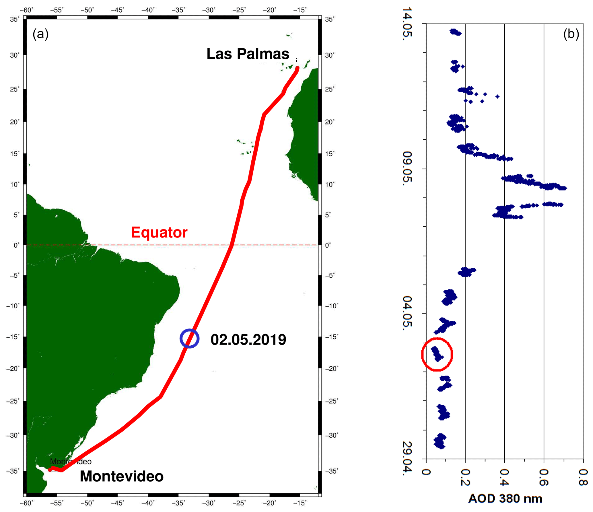
Figure 1 (a) Ship route from Montevideo to Las Palmas. The blue circle indicates the location of the measurements used in this study. (b) Aerosol optical depth at 380 nm measured with a hand-held Sun photometer.

In this study, we minimise these difficulties by using atmospheric observations in the presence of very low aerosol loads. During a ship campaign across the tropical Atlantic, very low aerosol optical depth (AOD) was observed on one day (2 May 2019). At 360 nm (the wavelength at which we analyse the atmospheric O₄ absorption), the AOD ranged from 0.034 to 0.056, which is an order of magnitude lower than the optical depth of molecular Rayleigh scattering.

Like in previous studies, we compare the observed atmospheric O₄ absorption with the results of radiative transfer simulations. Information about the aerosol properties is derived from Sun photometer measurements in combination with ceilometer measurements. Also in our study, considerable uncertainties about the aerosol vertical profile and the aerosol optical properties exist. However, these uncertainties are less important for the interpretation of the comparison results than in previous studies because of the low AOD, and we find large discrepancies between the measured and simulated O₄ absorptions.

The paper is organised as follows. In Sect. 2, an overview of the ship campaign and the instruments used in this study is given. Sections 3 to 5 describe the spectral analysis, the cloud classification and the calculation of the O₄ profile. In Sect. 6, the radiative transfer simulations and the extraction of the aerosol extinction profiles are presented. Section 7 presents the comparison results, and Sect. 8 the summary and conclusions.

2 Overview of the ship campaign and the instruments used in this study

The MAX-DOAS measurements were carried out during a cruise (MSM82/2) of the German research vessel (RV) Maria S. Merian (https://www.ldf.uni-hamburg.de/merian.html, last access: 1 May 2021) from Montevideo (Uruguay) to Las Palmas (Spain) from 26 April to 14 May 2019 (see Fig. 1). More details on the ship cruise MSM82/2 can be found in Krastel et al. (2019). In this study, we focus on one day with particularly low AOD (2 May), which is marked in Fig. 1.

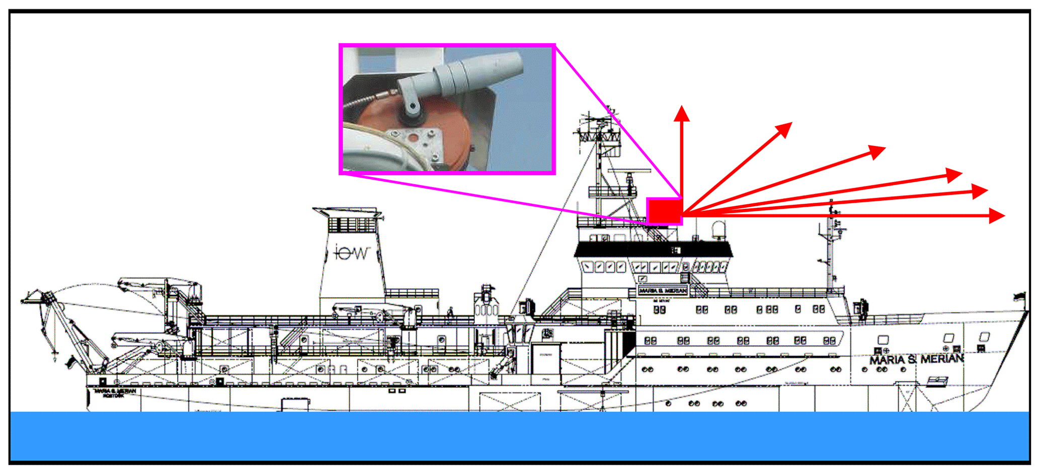
Figure 2 The position and viewing direction of the MAX-DOAS instrument on the RV Maria S. Merian during the ship cruise (ship drawing taken from https://briese-research.de/research-department/research-vessels/rv-maria-s-merian, last access: 1 May 2021).

The MAX-DOAS instrument was mounted above the ship's bridge at about 20 m altitude above sea level. The telescope was aligned in the driving direction of the ship (Fig. 2).

2.1 MAX-DOAS instrument

The MAX-DOAS instrument is a so-called Tube MAX-DOAS instrument which was developed and built by the electronic workshop of the Max Planck Institute for Chemistry in Mainz (Donner, 2016). It consists of two major parts: the telescope unit and the spectrometer unit. The telescope unit is mounted outside on the railing of the ship. The spectrometer unit is located inside the ship. Besides the spectrometer it also contains a peltier cooling element which stabilises the spectrometer temperature at 15 ^∘C. Both units are connected via a quartz glass fibre bundle and electric cables. The telescope unit is equipped with a gyroscope to stabilise the elevation angles by continuously adjusting the motor position with an accuracy of $\pm \mathrm{0.1}{}^{\circ }$.

The spectrometer is an Avantes ULS2048x64-USB2. It covers the spectral range from 299.4 to 463.1 nm with a spectral resolution between 0.52 and 0.54 nm as described by the full width at half maximum (FWHM). Spectra are measured with an integration time of 1 min at the following elevation angles: −2, −1, −0.5, 0, 0.5, 1, 2, 3, 4, 5, 6, 8, 10, 15, 30, 90^∘. Note that in this study only measurements with positive elevation angles are used. One elevation sequence is completed within about 21 min. Dark current and offset spectra are taken during nighttime and are used to correct the measured spectra before the spectral analysis.

2.2 Sun photometer

A MICROTOPS II Sun photometer provided atmospheric totals on aerosol and water vapour. The instrument, when directed towards the Sun (in a hand-held operation), captures via diodes the solar intensity in five subspectral bands near wavelengths of 380, 440, 675, 870 and 940 nm. In combination with the larger reference solar intensity at the top of the atmosphere – using time and (GPS-provided) position data – Sun photometer measurements define the atmospheric attenuation at these solar subspectral bands. Four spectral bands (near 380, 440, 675 and 870 nm) sample in trace-gas-poor regions, while one spectral band (near 940 nm) is strongly affected by water vapour absorption. In the absence of clouds, the solar attenuations in the four trace-gas-poor bands can be linked to aerosol – after (surface air pressure defined) contributions from air-molecule (Rayleigh) scattering have been removed. Hereby, the aerosol associated attenuations are quantified by the (vertically normalised) aerosol optical depth (AOD). As the instrument offers AOD values simultaneously at four different solar wavelengths, the typical aerosol particle size is revealed and even AOD contributions from submicrometre (mainly from pollution and wildfire) and supermicrometre size aerosol particles (mainly from dust and sea salt) can be distinguished. The determination of the atmospheric water vapour is based on the differential absorption between 870 and 940 nm attenuation data. Any quality measurement usually relies on many repeated samples in order to identify and remove poor data associated with Sun-view contamination by clouds and/or inaccurate orientations of the instrument into the Sun (which is done manually with the help of a pointing device). NASA's Aerosol Robotic Network (AERONET) subgroup of the Maritime Aerosol Network (MAN; Smirnov et al., 2009) provided the calibrated instrument for the cruise and also stores cruise data at https://aeronet.gsfc.nasa.gov/new_web/cruises_new/Maria_Merian_19_0.html (last access: 1 May 2021).

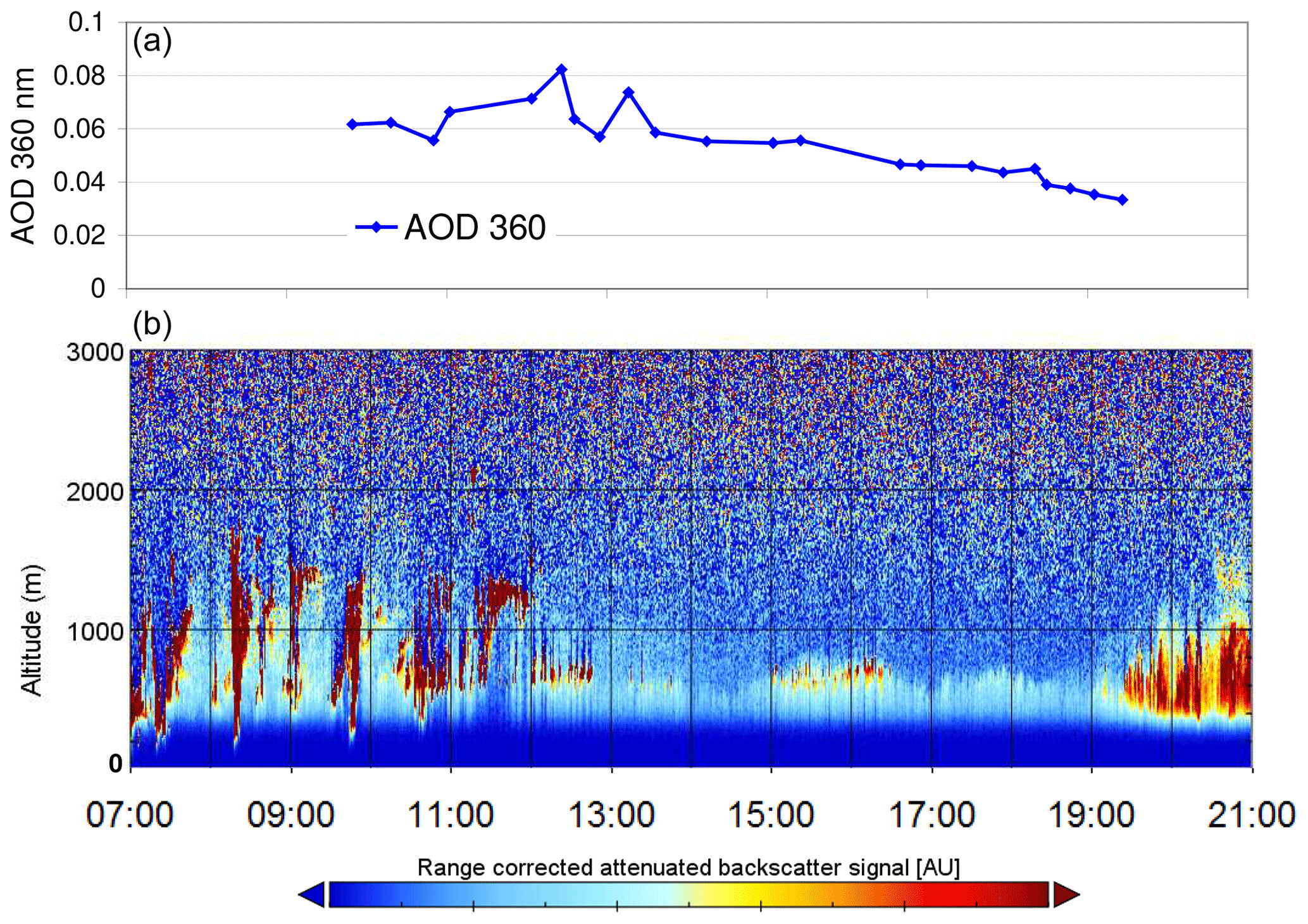
Figure 3 (a) AOD at 360 nm measured from the hand-held Sun photometer. The data were extrapolated from the measurements at 380 nm using the Ångström coefficient calculated from 380 and 440 nm. (b) Range-corrected ceilometer backscatter profile at 1064 nm.

The AOD at 360 nm for 2 May 2019 is shown in Fig. 3. Other results from the Sun photometer measurements (AODs at different wavelengths, Ångström exponents and fine- and coarse-mode AODs) are presented in Fig. A3.

Note that the uncertainties of the last AOD measurement on 2 May 2019, 19:26 UTC, are rather large because of the high solar zenith angle (SZA) of 85^∘. In particular, it was found that for that measurement the AOD from the fully processed Sun photometer data (Fig. A3) was about 30 % larger than the AOD of the initial retrieval (Fig. 3), while the results for all other measurements are almost identical. The radiative transfer simulations presented below for the last elevation sequence (19:06 to 19:25 UTC) are based on the initial (low) AOD values, which are in agreement with AOD measurements 20 min earlier. Nevertheless, the comparison results for this last elevation sequence should be treated with caution because of the large uncertainties of the corresponding AOD measurement.

2.3 Ceilometer

The Jenoptik 15k ceilometer of the Max Planck Institute for Meteorology (MPI-M) is a simple laser system operating at 1064 nm at an invisible trace-gas-free near-IR wavelength. Laser impulses are sent upward into the atmosphere, and based on strength and delay of backscattered return signals altitude positions for atmospheric aerosol and clouds are derived. Due to their stronger backscatter at optically thicker media, such as clouds, overhead cloud base altitudes are well captured. However, as laser light strongly attenuates in optically thicker media, no information above a cloud base is possible. Vertical profiles of aerosol for clouds-free views (and below clouds) are possible up to about 7 km in altitude during the night but only up to about 4 km in altitude during the day, due to scattering noise by sunlight. No useful aerosol profiling is possible near the surface (e.g. lower 300 m), because the signal sender and receiver are not at an identical location. Recorded ceilometer data of the cruise are accessible via an anonymous ftp site at ftp://ftp-projects.zmaw.de/aerocom/ships/ceilometer_MSM/ (last access: 1 May 2021).

Table 1 Settings for the DOAS analysis of O₄.

3 Spectral analysis

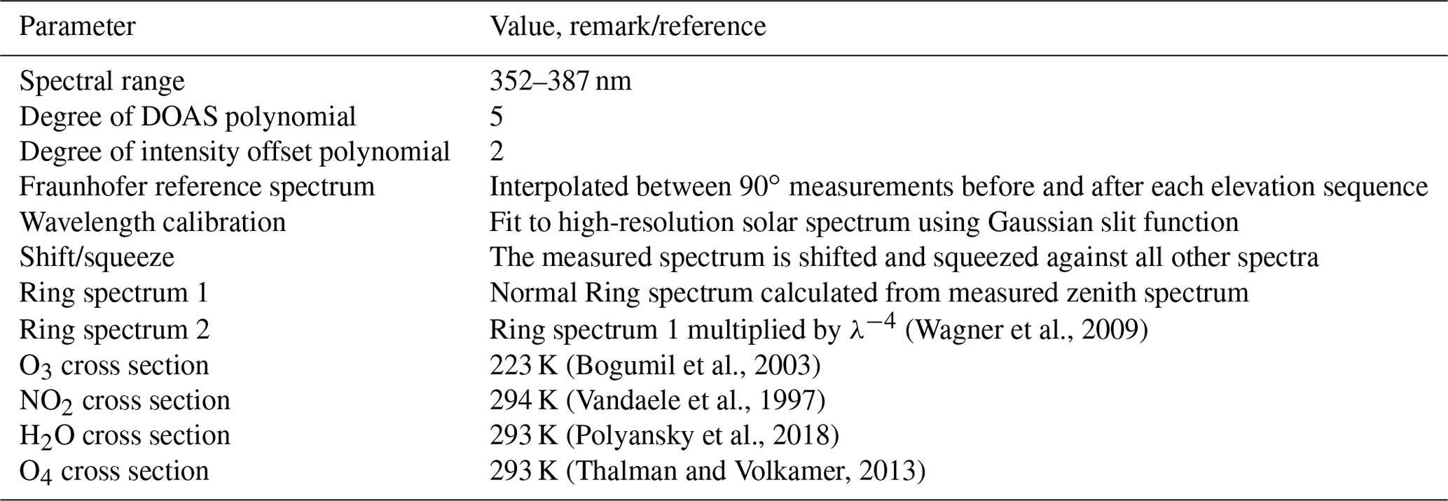
The spectral analysis is performed following mostly the settings suggested by Wagner et al. (2019). The spectral range from 352 to 385 nm is chosen, which contains two O₄ absorption bands. Note that in Wagner et al. (2019), the wavelength range of 352–387 nm was used. Here, we restricted it to 352–385 nm, because for some measurements (not on 2 May 2019) large spectral structures were found > 385 nm). For 2 May 2019, almost identical results (differences < 1 %) were found for both spectral ranges. The details of the analysis are given in Table 1. Figure A1 (left) presents an example of the spectral analysis as used in this study. In addition to the other cross sections, also an H₂O cross section (Polyansky et al., 2018) is included. The reason for including an H₂O cross section as well as the effect of including a second O₄ cross section are discussed in Appendix A1.

The results of the spectral analysis represent the integrated trace gas concentration along the atmospheric light path, the so-called slant column density (SCD). For O₄, the SCD is expressed with respect to the square of the O₂ concentration (see Greenblatt et al., 1990). Thus, the unit of the O₄ SCD is molec.² cm⁻⁵. For the analysis of the measured spectra, a so-called Fraunhofer reference spectrum is used. In this study, the Fraunhofer reference spectrum is calculated as the average of the zenith spectra before and after the chosen elevation sequence, weighted by the time of the selected measurement from that elevation sequence. Before performing the spectral analysis, these sequential Fraunhofer reference spectra are fitted to a “universal” Fraunhofer reference spectrum (29 April, 13:43 UTC; SZA: 44.8^∘, elevation angle: 90^∘) to transfer the spectral calibration of the universal Fraunhofer reference spectrum to the sequential Fraunhofer reference spectra. The universal Fraunhofer reference spectrum was calibrated using a high-resolved solar spectrum.

Since the Fraunhofer reference spectrum also contains atmospheric trace gas absorptions, the output of the spectral analysis represents the difference between the SCDs of the selected non-zenith spectrum and the Fraunhofer reference spectrum, the so-called differential SCD (or dSCD).

The typical fit error of the derived O₄ dSCD is between 2×10⁴¹ molec.² cm⁻⁵ and 4×10⁴¹ molec.² cm⁻⁵. Depending on the magnitude of the retrieved O₄ dSCD, this corresponds to relative errors between 1 % and 4 %.

4 Cloud detection using the MAX-DOAS measurements

Although during most of the afternoon on 2 May clear-sky conditions prevailed, also some scattered clouds were present. They were, e.g. detected by the ceilometer in zenith direction (see Fig. 3). In order to derive information about possible cloud contamination for the individual MAX-DOAS measurements, the MAX-DOAS measurements themselves were used for the detection of cloud contamination, similar to the method in Wagner et al., (2014, 2016). Figure A4 in the Appendix shows the time series of the retrieved O₄ dSCDs on 2 May for the different elevation angles. During the morning, the O₄ dSCDs show strong variability caused by the presence and variability of clouds as was also seen in the ceilometer data (Fig. 3). During the afternoon, for most of the time, smooth variations of the O₄ dSCDs are found, indicating clear-sky conditions. However, for some times and elevation angles, also small systematic deviations (usually reductions) of the O₄ dSCDs occur, which are caused by scattered clouds. During periods without any cloud contamination, the temporal variability of the retrieved O₄ dSCDs is rather small (scatter of the O₄ dSCDs is typically $\le \mathrm{5}\times {\mathrm{10}}^{\mathrm{41}}$ molec.² cm⁻⁵). Measurements with deviations > 10⁴² molec.² cm⁻⁵ compared to the extrapolated O₄ SCDs from the smooth (cloud-free) neighbouring measurements are thus flagged as cloud contaminated. From the 11 selected elevation sequences during the mainly cloud-free periods in the afternoon of 2 May, seven are found to be completely free of cloud contamination.

5 Calculation of the O₄ profile and O₄ VCD

The O₄ height profile and vertical column density (VCD) for 2 May 2019 are calculated from vertical profiles of temperature and pressure. Also the effect of the atmospheric humidity is accounted for. For the profiles of temperature, pressure and atmospheric humidity, we used the results from the ECMWF ERA-Interim data set (Berrisford et al., 2011) for 2 May 2019. From the temperature and pressure profiles, the air concentration [air] is calculated. Then the O₂ concentration [O₂] is derived according to the following equation:

$$\begin{array}{}\text{(1)}& \left[{\mathrm{O}}_{\mathrm{2}}\right]=\left[\text{air}\right]\cdot M_{{\mathrm{O}}_{\mathrm{2}}}\cdot \left(\mathrm{1}-M_{{\mathrm{H}}_{\mathrm{2}}\mathrm{O}}\right).\end{array}$$

Here, $M_{{\mathrm{H}}_{\mathrm{2}}\mathrm{O}}$ is the mixing ratio of water vapour taken from the ERA-Interim data. For the dry air mixing ratio of O₂ ($M_{{\mathrm{O}}_{\mathrm{2}}})$, a value of 21 % is assumed. The O₄ concentration is then represented by the square of the O₂ concentration (Greenblatt et al., 1990). To derive the O₄ VCD, the O₄ concentration is vertically integrated between the surface and 30 km with a vertical resolution of 20 m.

The temperature and pressure from the ECMWF ERA-Interim data set at the surface are also compared to the in situ measurements on the ship. It is found that the ECMWF temperature is slightly lower (−0.7 K) and the ECMWF pressure is slightly higher (+2 hPa) than the corresponding in situ measurements; see Fig. A5 in the Appendix. Therefore, we repeated our calculations of the O₄ profiles by shifting the ECMWF values for the whole profiles by +0.7 K and −2 hPa. The resulting change of the O₄ VCD is rather small (+0.3 %). The derived O₄ VCD for the modified profile is (1.245±0.25) × 10⁴³ molec.² cm⁻⁵. The most probable reasons for the discrepancies are originating from the rather coarse horizontal (∼ 80 km) and temporal (6 h) resolution of the ECMWF ERA-Interim data set. First, the given model data are the average for the modelled box. Moreover, the simulation uncertainties are increased for parameterised subscale processes (e.g. wave motion) which do affect the in situ measurements.

To estimate the uncertainty of the derived O₄ VCD, the temperature and pressure of the whole profiles are varied by ±2 K and ±2 hPa, respectively. The resulting changes of the O₄ VCDs are ±1.5 % and ±0.9 %, respectively. In addition, assuming an uncertainty of the atmospheric humidity profile of 30 % leads to an uncertainty of the derived O₄ VCD of 0.9 %. Thus, we estimate the total uncertainty of the O₄ VCD to ±2 %.

Finally, a subtle detail should be mentioned: the integration of the O₄ VCD was performed starting from sea level, while the instrument was located about 20 m a.s.l. This rather small difference would result in a reduction of the O₄ VCD by 0.4 %. However, this effect is considered in exactly the same way in the radiative transfer simulations, where the instrument was also put at an altitude of 20 m, while the O₄ air mass factors (AMFs) are calculated for the O₄ column starting from sea level. Thus, it is a consistent procedure to use the O₄ VCD integrated from sea level for the conversion of the measured O₄ dSCDs into O₄ differential air mass factors (dAMFs).

Table 2 Vertical resolution used for the radiative transfer simulations.

6 Radiative transfer simulations

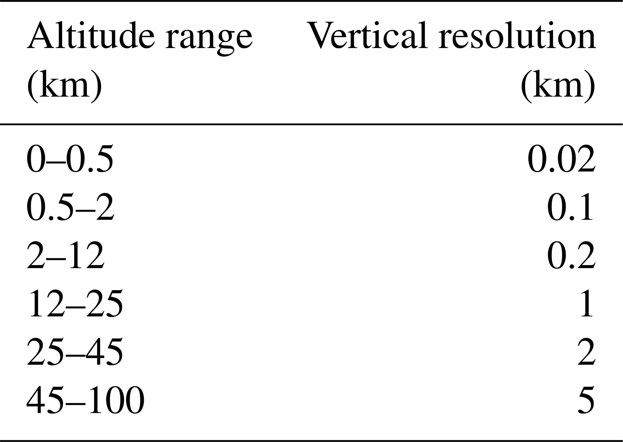
O₄ dSCDs are calculated using the full spherical Monte Carlo radiative transfer model MCARTIM (Deutschmann et al., 2011). For the simulations, the profiles of temperature, pressure and O₄ as described in Sect. 5 are used. The vertical resolution was set to 20 m close to the surface and increases with altitude (see Table 2). The surface albedo was set to 0.05. The value of 5 % was chosen to be consistent with the Mainz profile algorithm (MAPA) inversions, and because it is appropriate for many parts of the global ocean. However, by having a closer look at maps of albedo (Kleipool et al., 2008) and chlorophyll content (e.g. from the NASA Earth Observatory: https://earthobservatory.nasa.gov/global-maps/MY1DMM_CHLORA, last access: 1 May 2021), we found that at the specific location of the measurements, very clear waters exist, for which the surface albedo is typically higher (about 7 % to 8 %). The presence of very clear waters was also supported by the in situ chlorophyll measurements aboard the ship. We therefore made additional radiative transfer simulations using a surface albedo of 8 %. We found that the obtained O₄ dAMFs were almost identical with those for 5 % surface albedo (differences < 1 %). The reason for the good agreement is that the effect of the surface albedo is similar for the O₄ AMFs for different elevation angles. Thus, the effect of varying surface albedo almost cancels out.

The simulations were performed for the exact SZA and relative azimuth angles of the individual measurements. From the obtained O₄ AMFs, the corresponding O₄ dAMFs are calculated by subtracting the simulated O₄ AMFs for the zenith viewing direction. To achieve the best consistency with the measurements, for the simulation of the zenith measurements (interpolated between the zenith observations before and after the sequence) the SZA and relative azimuth angle for the exact time of the non-zenith measurements are also used for the simulations of the zenith measurements. The temporal evolution of the SZA and relative azimuth angle for 2 May are shown in Fig. A6 in the Appendix.

It should be noted that it is important to use a consistent treatment of the SZA and relative azimuth angles in the simulations and measurement analyses. Especially the choice of the Fraunhofer reference spectra is important. If, e.g. either zenith measurements before or after the selected elevation sequence are used as reference spectra, systematic deviations of the retrieved O₄ dSCDs of up to 10 % can occur (see Fig. A7 in the Appendix).

O₄ dAMFs are simulated for two aerosol extinction profiles as well as for a pure Rayleigh atmosphere. For the extraction of the aerosol extinction profiles, the observations by the Sun photometer and the ceilometer were used (see Sect. 6.1). For the simulations including aerosols, the phase function is represented by a Henyey–Greenstein (HG) parameterisation with an asymmetry parameter of 0.68. The single scattering albedo was set to 0.95. Variations of these properties lead to changes of the simulated O₄ dSCDs by up to ±3 % (see Fig. A8 in the Appendix). These rather low uncertainties are related to the low AOD on 2 May 2019. For measurements with higher aerosol loads, the corresponding uncertainties are usually much larger (e.g. Wagner et al., 2019). Here, it should be noted that the HG phase function model is a rather simplified approximation for true aerosol phase functions. Thus, especially for measurements with small scattering angles (e.g. around noon on 2 May 2019), the uncertainties of the radiative transfer model (RTM) simulations might be larger.

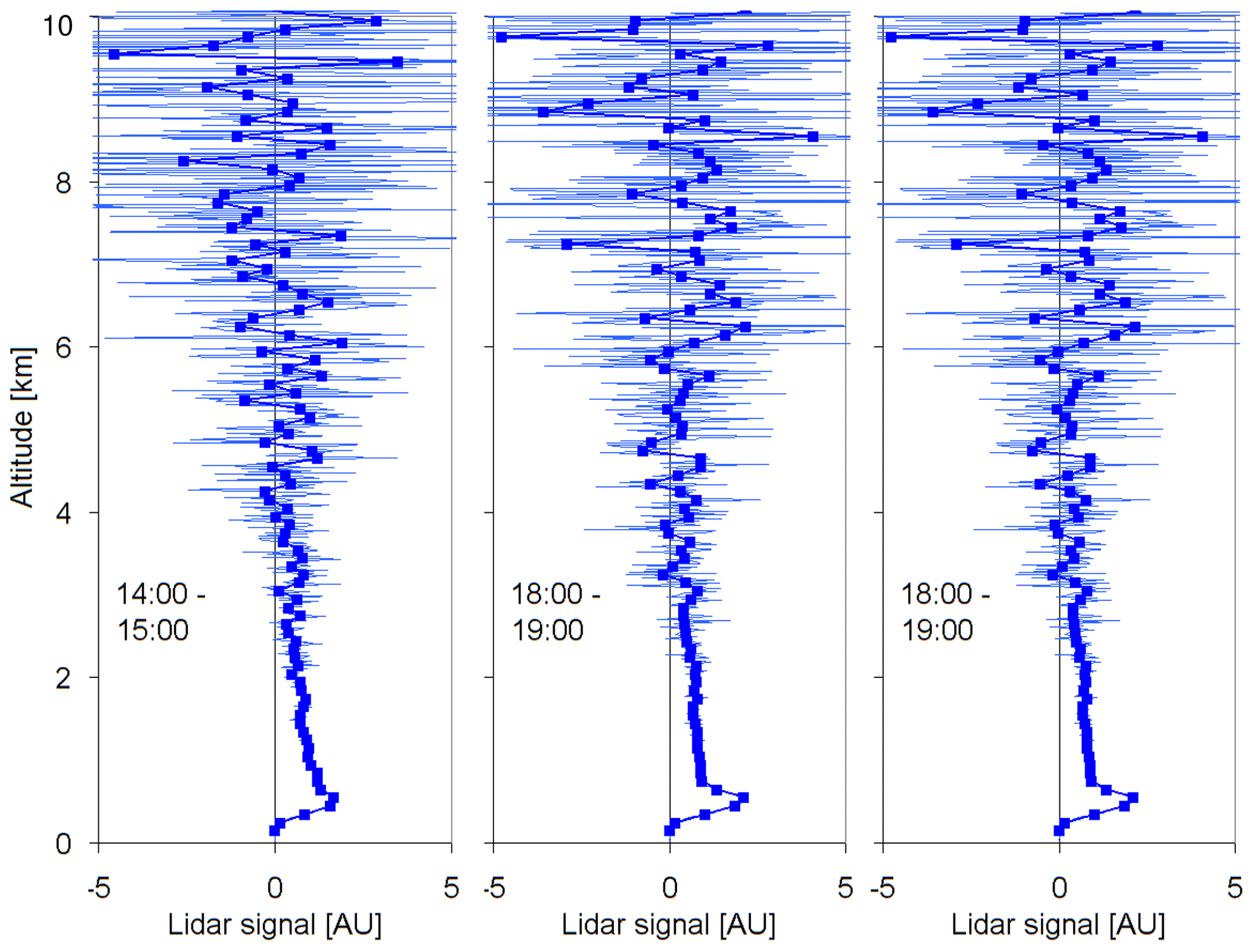
Figure 4 Hourly averaged and range-corrected ceilometer backscatter profiles for three periods on 2 May 2019 without cloud contamination. The thin lines represent the raw data. The dotted lines represent the smoothed profiles (averages over 100 m). The scatter of the range-corrected backscatter profiles increases because the received raw signal scales with the inverse of the square of the distance.

6.1 Extraction of the aerosol extinction profiles

Figure 4 presents the hourly averaged and range-corrected ceilometer backscatter profiles for three periods in the afternoon on 2 May 2019 without cloud contamination. In a first-order approximation, these backscatter profiles are proportional to the aerosol extinction. Thus, together with the total AOD from the Sun photometer measurements, the aerosol extinction profiles can be determined. However, ceilometer measurements are affected by several instrumental limitations, which complicate the direct conversion to aerosol extinction profiles:

• a.

  Due to the missing overlap between the outgoing beam and the field of view of the detector, the sensitivity of the ceilometer is very low for altitudes below 500 m. Thus, for this altitude range, no information on the aerosol extinction can be derived from the ceilometer measurements.

• b.

  In spite of the long averaging period, strong noise still appears for altitudes above 3 km.

Due to these limitations, the ceilometer profiles can only be used for a restricted altitude range. In the following, we used the ceilometer profiles for the altitude range between 500 m and about 7 to 9 km. Between 500 and 3000 m, averages for 100 m layers are calculated. Below 500 m, the values at 500 m are either set constant for the layer below or are linearly extrapolated from the ceilometer data between 500 and 800 m (similar to the method in Wagner et al., 2019). Since between 3 and 10 km the noise increases strongly, a third-order polynomial was fitted to the ceilometer data in that height range. The polynomial values are used for the altitude range for which positive values are obtained. Between 7 and 9 km, the polynomial values for the three profiles cross zero. Above these altitudes, the profile values are set to zero. These extraction steps are illustrated in Fig. A9 in the Appendix. The exact choice of the altitude, at which the extinction is set to zero, has negligible influence on the simulated O₄ dAMFs.

Before the backscatter profiles are normalised with the total AODs measured by the Sun photometer, the stratospheric part of the total aerosol profile has to be added. This step is usually not important, because in more polluted areas the total AOD is clearly dominated by the tropospheric part. However, for our study, the total AOD is so low that the stratospheric part constitutes a substantial fraction (up to 25 %) of the total AOD. Thomason et al. (2018) report the stratospheric AODs in the tropics at 525 nm to be about 0.005 to 0.006. Assuming an Ångström exponent of 2 (e.g. Malinina et al., 2019), the corresponding AOD at 360 nm is estimated to around 0.011 and 0.013. In the following, we used a value of 0.012. Here, it should be noted that the Ångström exponent for stratospheric aerosols is usually derived for wavelengths at and above 525 nm. Thus, it is not clear how representative the used value of 2 also is for shorter wavelengths. To estimate the uncertainties of the simulated O₄ dSCDs related to the uncertainty of the Ångström exponent, we performed additional radiative transfer simulations assuming a stratospheric AOD of 0.008 (corresponding to an Ångström exponent of about 1). We found that the O₄ dSCDs differ from those for a stratospheric AOD of 0.012 by less than 1 %.This stratospheric AOD (0.012) is then subtracted from the total AOD (Fig. 3) measured by the Sun photometer. Then the tropospheric aerosol profiles (as described above; see also Fig. A9) are normalised by the resulting tropospheric AOD. Finally, the stratospheric extinction profile is added to the normalised tropospheric aerosol extinction profiles. For the stratospheric extinction profile, we used a simplified shape with an AOD of 0.012. Here, it is important to note that the details of the extinction profile in the upper troposphere and stratosphere are not critical. For example, the simulated O₄ dAMFs using aerosol profiles with or without the stratospheric part are almost the same. The final aerosol extinction profiles used for the RTM simulations are shown in Fig. 4.

Since the aerosol properties can change with altitude, the relative profile shape measured at 1064 nm might differ from the aerosol extinction profile at 360 nm. In order to estimate the effect of the varying aerosol profiles at both wavelengths, we performed additional radiative transfer simulations using modified tropospheric aerosol profiles. The aerosol extinction in the lowest 1000 m of the extracted profiles was changed by ±20 %, and the free tropospheric part above was adjusted to keep the total AOD unchanged. The resulting O₄ dAMFs were almost unchanged for elevation angles > 4^∘. For lower elevation angles, the changes were found to be ±2 %.

6.2 Calculation of effective temperatures for the O₄ absorption

Since the temperature of the troposphere decreases with altitude, and the O₄ absorption cross section depends on temperature, the retrieved O₄ dSCDs might deviate from the true O₄ dSCDs (the integrated O₄ concentration along the atmospheric light paths), because only one O₄ cross section for a fixed temperature is used in the spectral analysis. Thus, before the O₄ dAMFs from the measured spectra are compared to those from the radiative transfer simulations, the effect of the temperature dependence of the O₄ absorption has to be investigated.

The effective temperature of the O₄ measurements is calculated according to

$$\begin{array}{}\text{(2)}& T_{\text{eff},\mathit{\alpha }}={\displaystyle \frac{\sum _z[{\mathrm{O}}_{\mathrm{4}}{]}_z\cdot ({\text{bAMF}}_{z,\mathit{\alpha }}-{\text{bAMF}}_{z,\mathrm{90}{}^{\circ }})\cdot T_z}{\sum _z[{\mathrm{O}}_{\mathrm{4}}{]}_z\cdot ({\text{bAMF}}_{z,\mathit{\alpha }}-{\text{bAMF}}_{z,\mathrm{90}{}^{\circ }})}}.\end{array}$$

Here, [O₄]_z represents the O₄ concentration at altitude z, bAMF_z,α the box AMF for elevation angle α at altitude z and T_z the temperature at altitude z. T_eff,α is the effective temperature for the measured O₄ dSCD at elevation angle α.

Equation (2) is applied for each individual measurement; the results are shown in Fig. A10. The effective temperatures range from 276 to 299 K. They depend systematically on the elevation angle and SZA. Measurements at low elevation angles are most sensitive for the layers near the surface, at which the highest temperatures occur. Measurements at high SZA (towards the end of the considered time period) have higher sensitivities for higher atmospheric layers with colder temperatures. Both dependencies are well represented by the results shown in Fig. A10.

To correct the effect of the temperature dependence, the correction factors presented in Fig. 13 in Wagner et al. (2019) are applied to the O₄ dSCDs retrieved with the O₄ cross section for 293 K. The corrected O₄ dSCDs differ by up to a few percent (between −2 % and +7 %) from the original O₄ dSCDs. In Fig. A11 in the Appendix, the effect of the temperature correction is shown for two selected elevation sequences. For the comparison with the radiative transfer simulations, the temperature-corrected O₄ dSCDs (or dAMFs) are used.

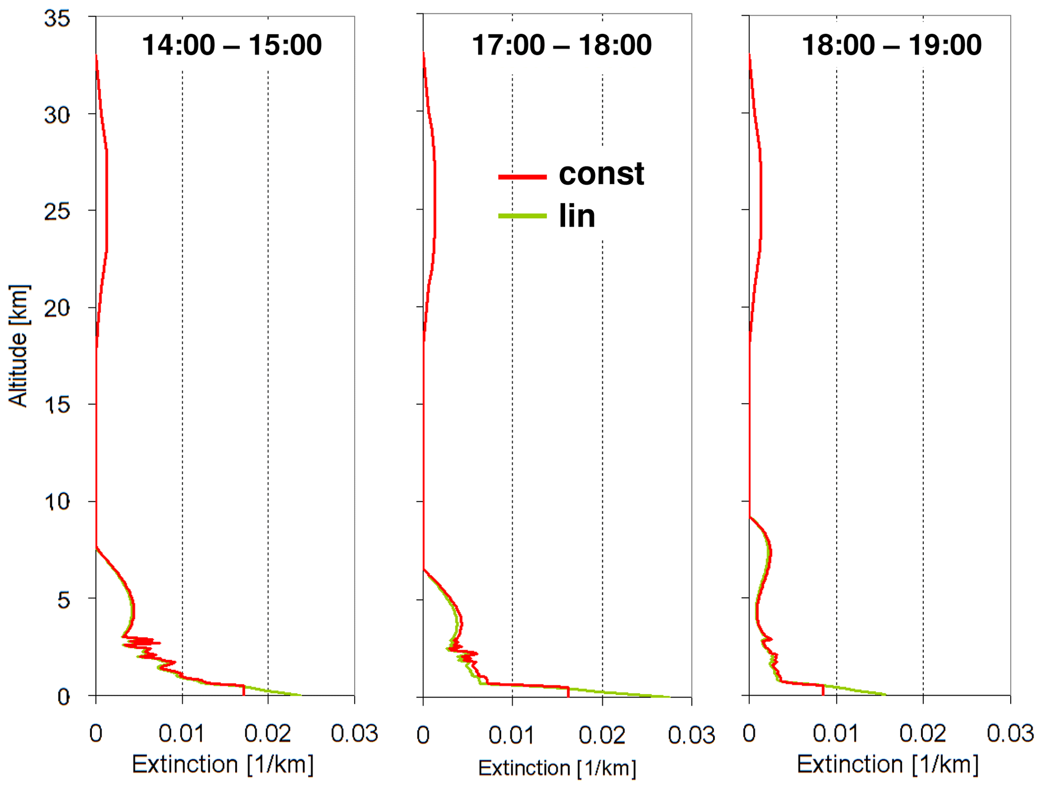
Figure 5 Complete aerosol extinction profiles for the three time periods without clouds after all corrections are applied. The green curves represent the profiles with linear extrapolation below 500 m; the red curves represent profiles with constant values below 500 m.

7 Comparison results

7.1 Direct comparison between measurements and RTM results

In Fig. 6, the O₄ dAMFs derived from the MAX-DOAS measurements are compared to those obtained from the radiative transfer simulations for elevation sequences not affected by clouds (similar comparisons for the sequences with cloud-contaminated measurements are shown in Fig. A12 in the Appendix).

On the left side of Fig. 6, the results from radiative transfer simulations without aerosols are shown. Here, for almost all cases, the measured O₄ dAMFs are systematically larger than the simulated O₄ dAMFs. This is an important finding, because especially for the low elevation angles, the presence of aerosol scattering leads to a decrease of the O₄ dSCDs. Thus, the simulations for a pure Rayleigh atmosphere represent an upper limit of the achievable O₄ dSCDs. Only for cloudy cases with a high probability for multiple scattering events could higher O₄ dSCDs occur, but such conditions can be ruled out here because of the absence of thick and vertically extended clouds. Thus, the overestimation of the simulated O₄ dSCDs for a pure Rayleigh atmosphere by the measured O₄ dSCDs indicates a fundamental inconsistency between measurements and simulations. Similar results are found for the elevation sequences with cloud contamination (Fig. A12 in the Appendix).

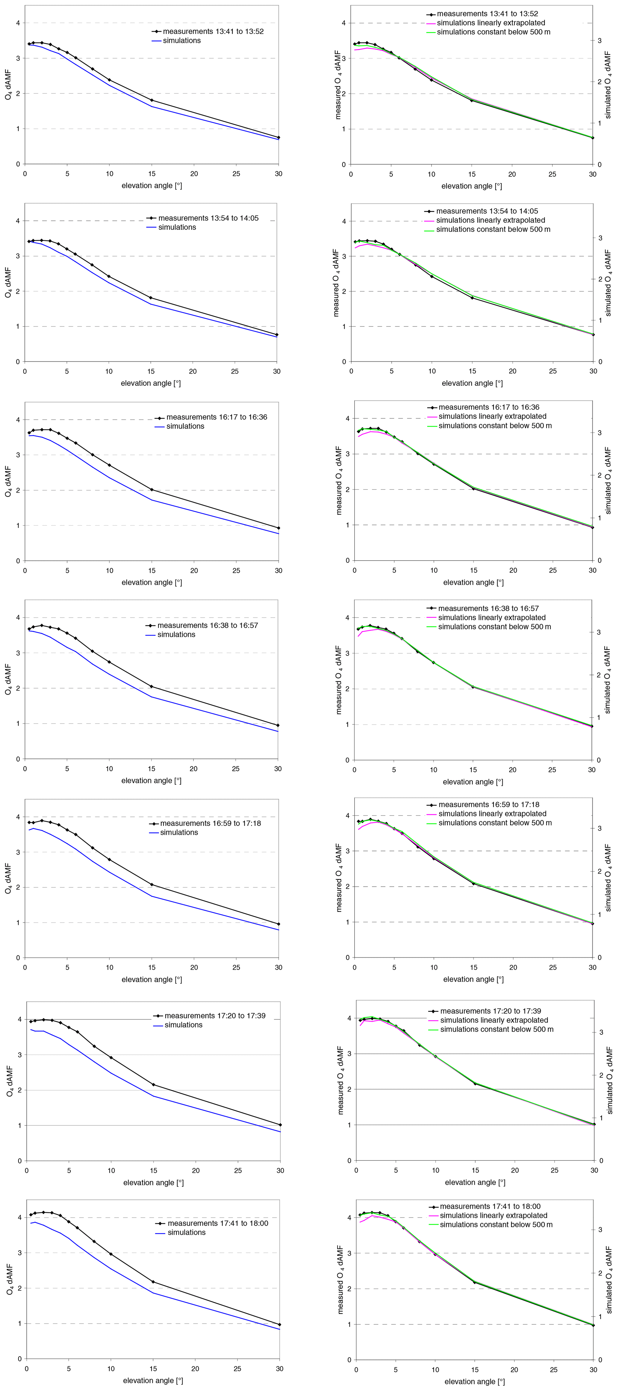
Figure 6 Comparison of the measured and simulated O₄ dAMFs for selected elevation sequences without cloud contamination. On the left side, the measured O₄ dAMFs are compared to simulations for a pure Rayleigh atmosphere. On the right side, they are compared to simulation results including aerosols (two profiles with either constant or linearly extrapolated aerosol extinction below 500 m). Note that in the right part, separate y axes on the right sides are used for the simulation results. The maxima of the right y axes are chosen to achieve the best agreement between the measured and simulated O₄ dAMFs (see text).

On the right side of Fig. 6, simulation results for the aerosol profiles ex tracted in Sect. 6.1 are shown. Note the separate y axes for the simulated O₄ dAMFs on the right side, for which the maxima are chosen to achieve the best agreement between the measured and simulated O₄ dAMFs. The exact values of the axis maxima were determined by fitting the measured O₄ dAMFs to the simulated O₄ dAMFs for elevation angles > 4^∘. For these elevation angles, the simulation results for the different profile shapes below 500 m are almost the same. Good qualitative agreement between measurements and simulation is found, especially for the aerosol profiles with constant extinction below 500 m. However, the absolute values differ strongly. The ratios between measured and simulated O₄ dAMFs are found to be between 0.8 and 0.86. Again, similar results are found for the elevation sequences with cloud contamination (Fig. A12 in the Appendix).

The scaling factors derived from this comparison between measured and simulated O₄ dSCDs are presented as blue data points in Fig. 7.

During the entire ship cruise, only during the beginning of 3 May 2019, similarly low (but still larger) AODs were measured compared to 2 May 2019. We compared the measured O₄ dAMFs for the first two elevation sequences on 3 May with radiative transfer simulations. For that comparison, we only made simulations for an aerosol-free atmosphere in order to limit the effort (and also because of the rapid temporal variation of the AOD during that time period). The results (see Fig. A13) are similar to those on 2 May 2019: except for the cloud contaminated measurements, the simulations are smaller than the measurements.

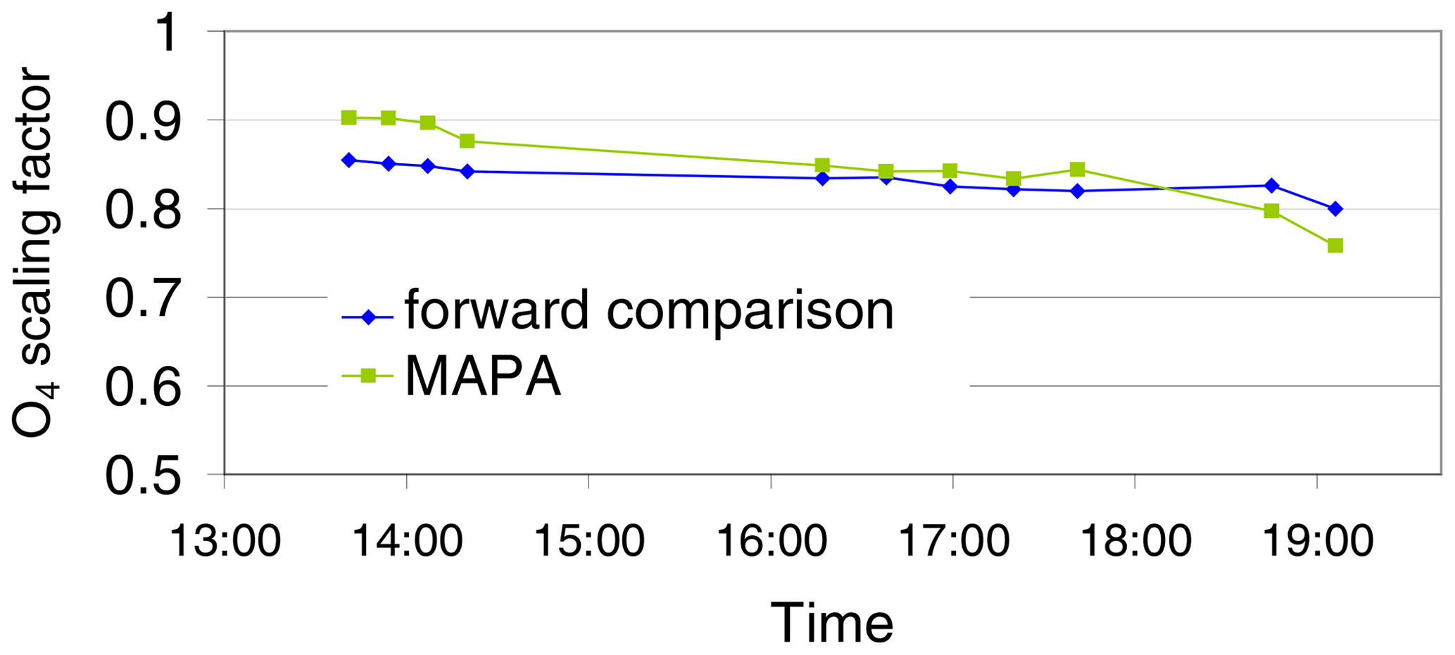
Figure 7 Scaling factors derived from the direct comparison between the measured and simulated O₄ dSCDs (blue) and from the MAPA profile inversion (green) for all elevation sequences shown in Figs. 6 and A12. Many of the measurements of the two last elevation sequences are affected by clouds. Note that for the last elevation sequence, the AOD used in the forward model has large uncertainties; see Sect. 2.2.

7.2 Profile inversion with MAPA

We also applied our profile inversion algorithm, MAPA (Beirle et al., 2019), to the measured O₄ dAMFs. For that purpose, a new MAPA look-up table (LUT) had to be created, because the lowest AOD in the original LUT (0.05) is larger than all AODs observed on 2 May 2020. The new LUT includes AOD values from 0 to 0.1 in steps of 0.02. MAPA provides the option to apply a fixed user-defined scaling factor or to determine a scaling factor yielding the best match between the forward model and measurement during profile inversion.

In Fig. A14 in the Appendix, the retrieved extinction profiles are shown for different scaling factors. Here, it should be noted that the individual measurements (not the sequences) with cloud contamination were skipped before the profile inversion. Only profiles with either “valid” or “warning” flags are shown (profiles with “error” flags are not shown). In Fig. A15 in the Appendix, the retrieved AODs for the different scaling factors are compared to the tropospheric AODs from the Sun photometer measurements (stratospheric AOD of 0.012 was subtracted). Also, the root mean square (rms) values between the measured and simulated O₄ dAMFs are shown (right). The colour of the MAX-DOAS inversion results indicates the quality of the profile inversion.

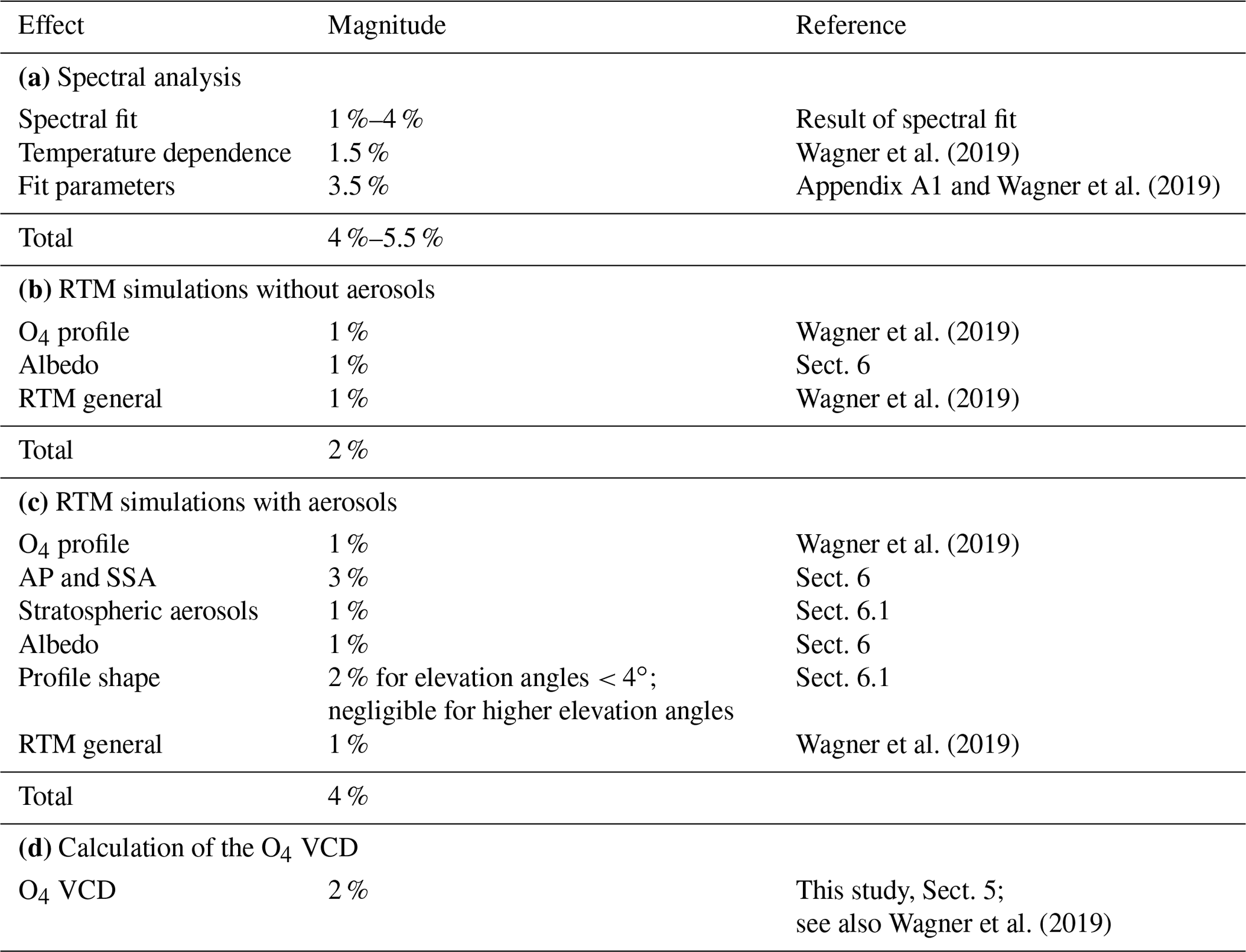
Table 3 (a) Uncertainties related to spectral analysis. (b) Uncertainties related to RTM simulations without aerosols. (c) Uncertainties related to RTM simulations with aerosols. AP indicates the asymmetry parameter and SSA indicates single scattering albedo. (d) Uncertainties related to calculation of the O₄ VCD.

Most valid profiles are obtained for scaling factors between 0.80 and 0.90, or for a free-fitted (variable) scaling factor. For the inversions with larger scaling factors, rather high rms values are found. For most cases, the retrieved AODs are smaller than those measured by the Sun photometer. For these low aerosol extinctions, the information content of the measurements is probably too low to constrain the aerosol extinction profiles, especially for high altitudes. Thus, also the retrieved AOD values are very unstable (see Fig. A15).

The obtained scaling factors are shown in Fig. 7. Overall good agreement between both comparison methods is found. For all elevation sequences, values of the scaling factor < 1 are found. For the direct comparison, the difference from unity is mostly larger than 15 % and thus cannot be explained by the uncertainties of the measurements and simulations, which are summarised in Table 3.

8 Conclusions

We compared measured and simulated O₄ absorptions for one day with very low aerosol optical depth. For such conditions, the uncertainties caused by imperfect knowledge of the aerosol properties play a smaller role than for comparison under more polluted conditions.

One important result of the comparison was that for all measurements, the observed O₄ absorption was higher than the simulation results for an atmosphere without aerosols. In the absence of optically thick clouds, the simulated O₄ dAMFs for an atmosphere without aerosols constitute an upper limit, since especially for the low elevation angles the inclusion of aerosols leads to a decrease of the O₄ absorption. The observed discrepancies thus indicate a fundamental inconsistency between simulations and measurements.

The measured O₄ absorptions are also compared to simulations including aerosol extinction profiles. The aerosol extinction profiles were constrained by measurements of the Sun photometer, the ceilometer and a climatology of stratospheric aerosols. Again, a large discrepancy was found for the absolute values. However, for the relative dependence of the O₄ dAMFs on the elevation angle, good agreement could be achieved. For each elevation sequence, the ratio of simulated and measured O₄ dAMFs was calculated. For that purpose, the elevation angles > 4^∘ were used, for which the O₄ dAMFs are almost insensitive to the profile shape in the lower atmospheric layers. For all elevation sequences, ratios of 0.85 or less were found. Similar ratios were also obtained from the application of our profile inversion algorithm (MAPA) to the measurements. The observed discrepancies cannot be explained by the uncertainties of measurements and/or simulations. Here, it is important to note that in the spectral analysis, we explicitly corrected for the (small) temperature dependence of the atmospheric O₄ absorption.

Our results indicate that something fundamental is missing or wrong in either the radiative transfer simulations or the spectral analysis of the atmospheric O₄ absorptions. We did not find a clear reason for the discrepancies. One possible reason for the discrepancies could be a systematically too small O₄ absorption cross section.

We recommend that similar studies under extremely low aerosol load should be made at different locations and during different seasons. Also O₄ absorptions at different wavelengths should be investigated.

Appendix A: Effect of including an H₂O cross section or a second O₄ cross section on the retrieved O₄ dSCDs

A1 H₂O cross section

Recent studies found evidence for substantial atmospheric H₂O absorptions in measured spectra in the UV range (Lampel et al., 2017; Wang et al., 2017, 2020). These absorptions are usually rather small, but especially for measurement conditions with high atmospheric humidity the inclusion of an H₂O cross section in the spectral analysis can be useful.

Figure A1 presents examples of the spectral analysis with either an H₂O cross section included or excluded. A clear H₂O absorption signal is found around 363 nm. The H₂O dSCDs retrieved at 363 nm agree reasonably well (r²=0.63) with those retrieved at 442 nm (see Fig. A2) with a similar slope (2.07) to that presented in Lampel et al. (2017), who found a slope of 2.39. If the H₂O cross section is not included in the analysis, a systematic structure appears in the residual. Thus, in this study, a water vapour cross section (Polyansky et al., 2018) is included in the spectral analysis. Here, it should be noted that compared to other locations, the water vapour absorption during the ship cruise was rather high because most of the measurements were carried out under conditions of high atmospheric temperature and humidity. At other, colder locations, the impact of the H₂O absorption might be negligible.

Although the H₂O absorption is clearly found in the spectral analysis, the effect of including an H₂O cross section or not on the retrieved O₄ dSCDs is still rather small. If an H₂O cross section is included, the retrieved O₄ dSCDs are about 2.5 % larger than without an H₂O cross section included.

A2 O₄ cross section at low temperature

We also investigated the effect of including a second O₄ cross section for low temperature (203 K). Before using this cross section in the fit, it was orthogonalised with respect to the O₄ cross section at 293 K. Including the additional O₄ cross section leads to only small changes of the retrieved O₄ dSCD of about −1.5 %. Here, it is interesting to note that the retrieved O₄ dSCDs for the O₄ cross section at low temperature were negative and the absolute values much smaller ($<\mathrm{2}\times {\mathrm{10}}^{\mathrm{43}}$ molec.² cm⁻⁵) than those at high temperature ($<\mathrm{6}\times {\mathrm{10}}^{\mathrm{43}}$molec.² cm⁻⁵). The largest negative O₄ dSCDs for the O₄ cross section at low temperature were found, indicating that the effective atmospheric temperatures decrease with elevation angle (see Sect. 6.2). Also, the correlation between both O₄ dSCDs (r²=0.20) is very low. Thus, we conclude that the measured spectra do not contain significant O₄ absorptions at low temperatures. For the interpretation of this finding, it should be noted that low temperatures exist only at higher atmospheric layers. The O₄ absorptions at these layers mostly cancel out in the spectral analysis, because the light paths of the measured spectra and the Fraunhofer reference spectra at these layers are very similar. This explains that the retrieved O₄ absorptions at cold temperatures are very small. To further confirm this hypothesis, we calculated the effective temperatures for the O₄ absorptions on 2 May 2019 (see Sect. 6.2) and found them to be very close to the temperature of the high temperature O₄ cross section (293 K). Based on these findings, the O₄ results in this study are retrieved without including a second O₄ cross section at low temperature. It should, however, be noted that for measurements at other locations and seasons including a second O₄ cross section in the spectral analysis might be meaningful.

Figure A1 Fit results for a spectrum taken on 2 May 2019, 13:14:50 UTC, at an elevation angle of 1^∘ (SZA: 33.6^∘). (a–c) Results if an H₂O cross section is included in the spectral analysis; (d–e) results if no H₂O cross section is included in the spectral analysis. The black lines represent the fitted cross section; the red lines indicate the residual (bottom) or the residual plus the fitted cross section.

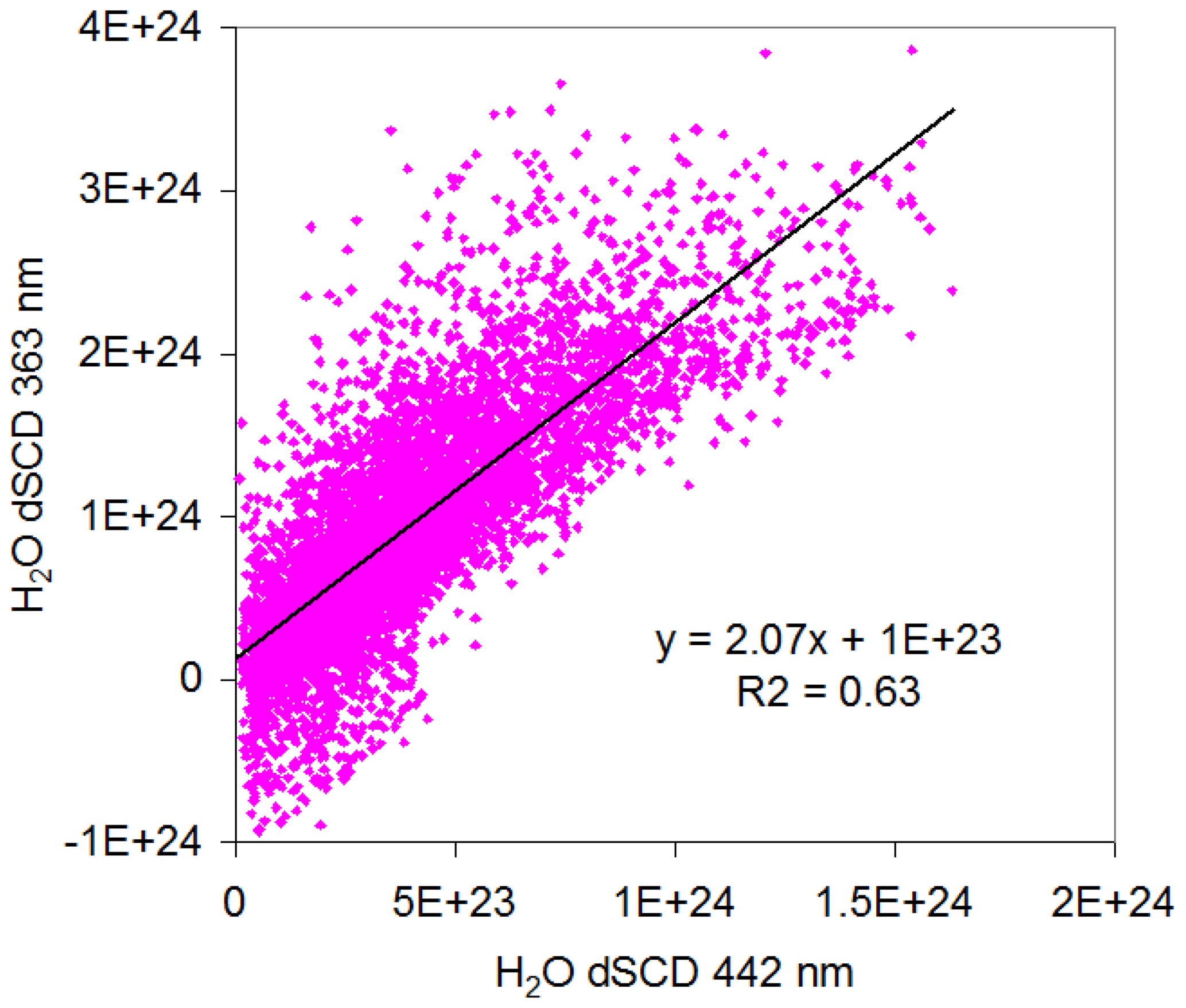
Figure A2 Correlation plot of the H₂O dSCDs retrieved at 363 nm versus those retrieved at 442 nm for the whole ship cruise. The regression line is fitted assuming that the H₂O dSCDs retrieved at 442 nm have no error.

A3 Additional figures

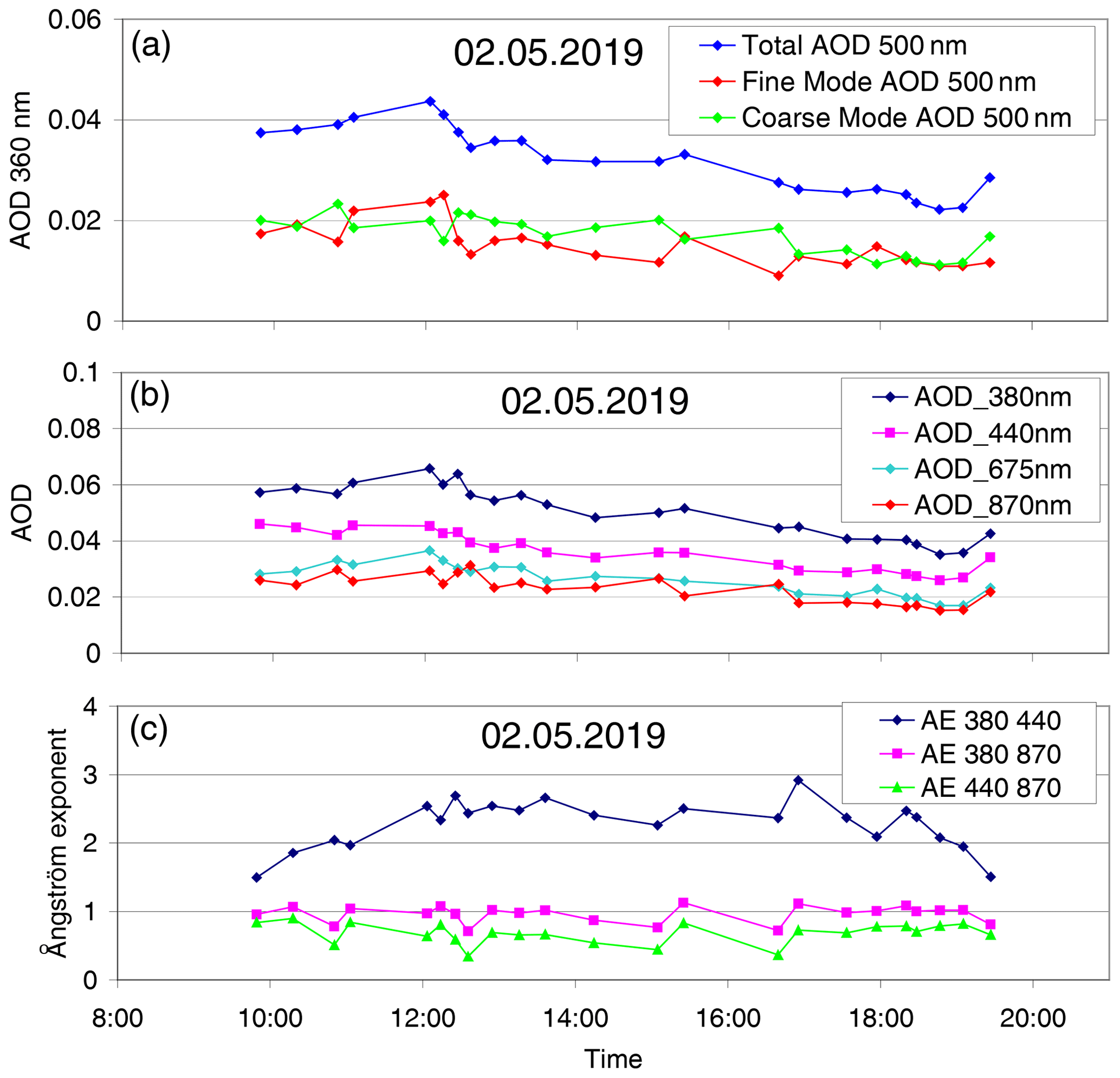
Figure A3 (a) AOD at 500 nm attributed to the coarse and fine modes, as well as total AOD. (b) Total AOD at different wavelengths. (c) Ångström exponents for selected wavelength pairs.

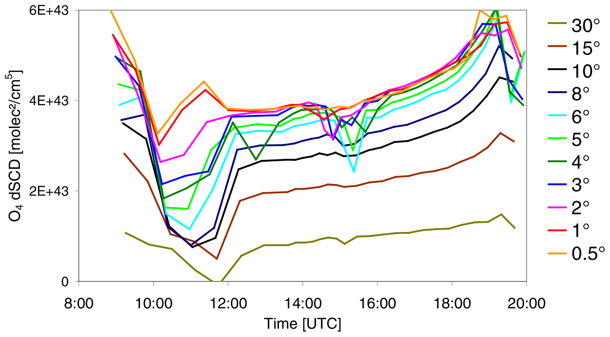
Figure A4 Time series of the retrieved O₄ dSCD on 2 May 2019 for the different elevation angles. During the afternoon, for most of the time, smooth variations are found. However, for some times and elevation angles, systematic deviations of the O₄ dSCDs occur, which are caused by scattered clouds.

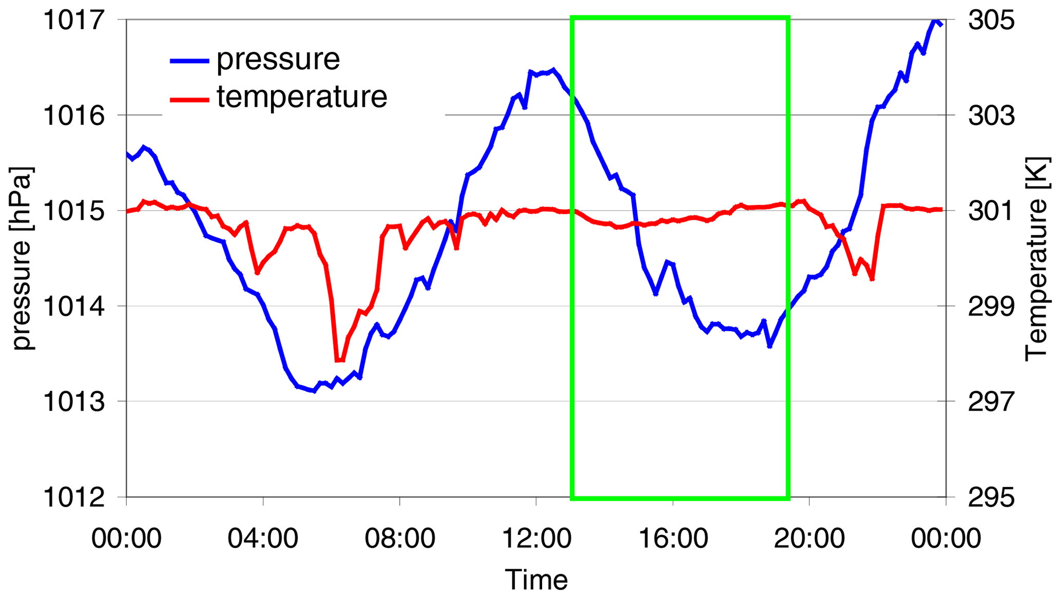
Figure A5 Diurnal variation of the surface pressure and temperature from in situ measurements on the ship. The green box indicates the period of the MAX-DOAS measurements used in this study. The corresponding values from the ECMWF model simulations are 1012.8 hPa and 299.8 K, respectively.

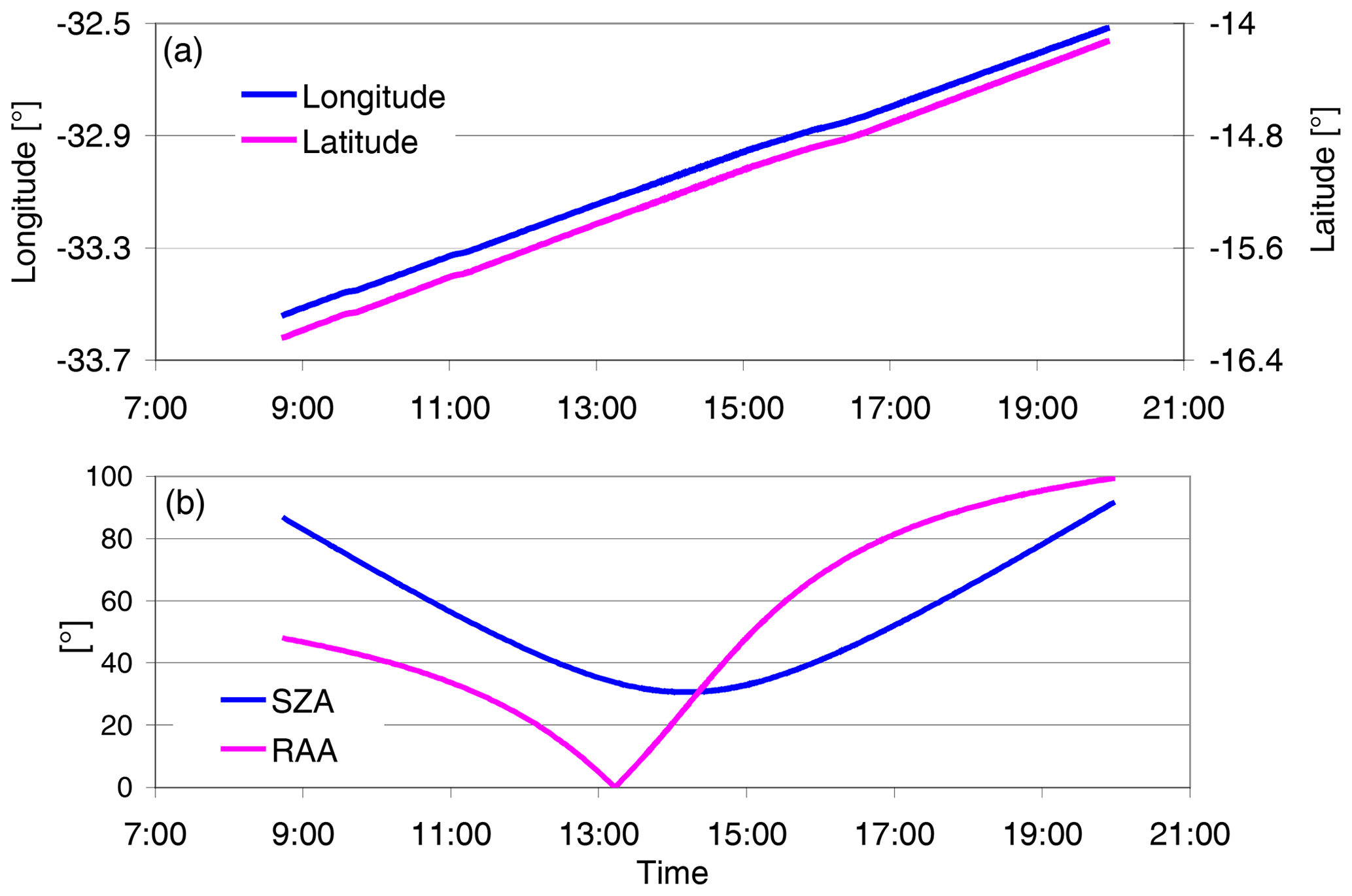
Figure A6 (a) Variation of the latitude and longitude of the ship position during 2 May 2019. (b) Corresponding variation of the SZA and relative azimuth angle (RAA).

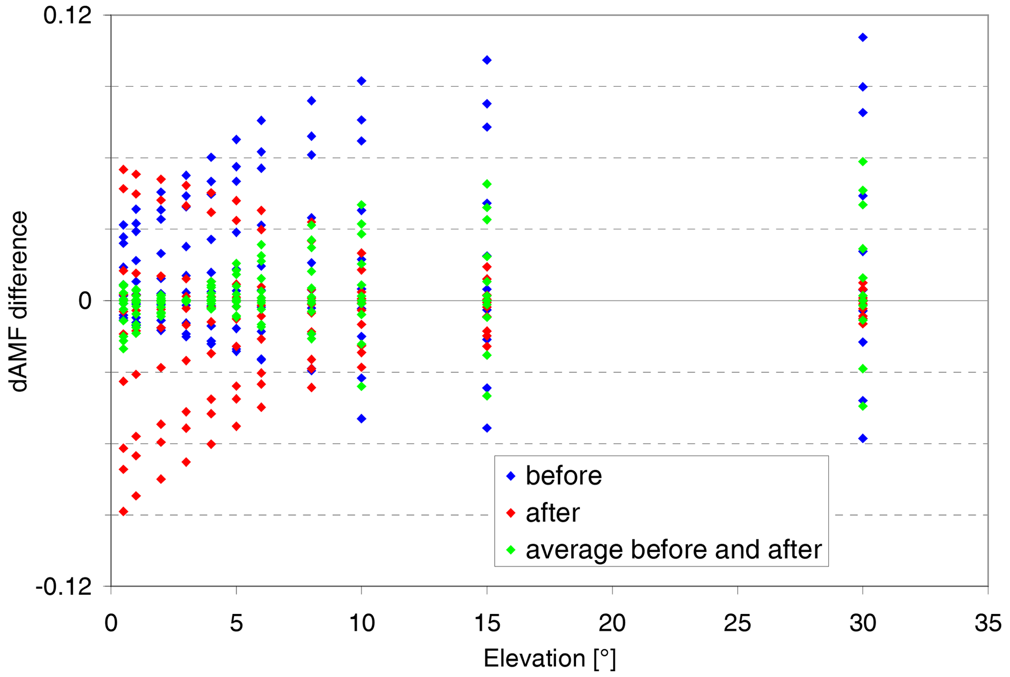
Figure A7 Effect of using different Fraunhofer reference spectra for the analysis of individual elevation sequences. Shown are the ratios of the obtained O₄ dSCDs for different selections versus those for Fraunhofer reference spectra interpolated between the zenith measurements before and after the selected elevation sequence. Before: zenith measurement before the sequence is used; after: zenith measurement after the sequence is used; average before and after: the average of the zenith measurements before and after the sequence is used.

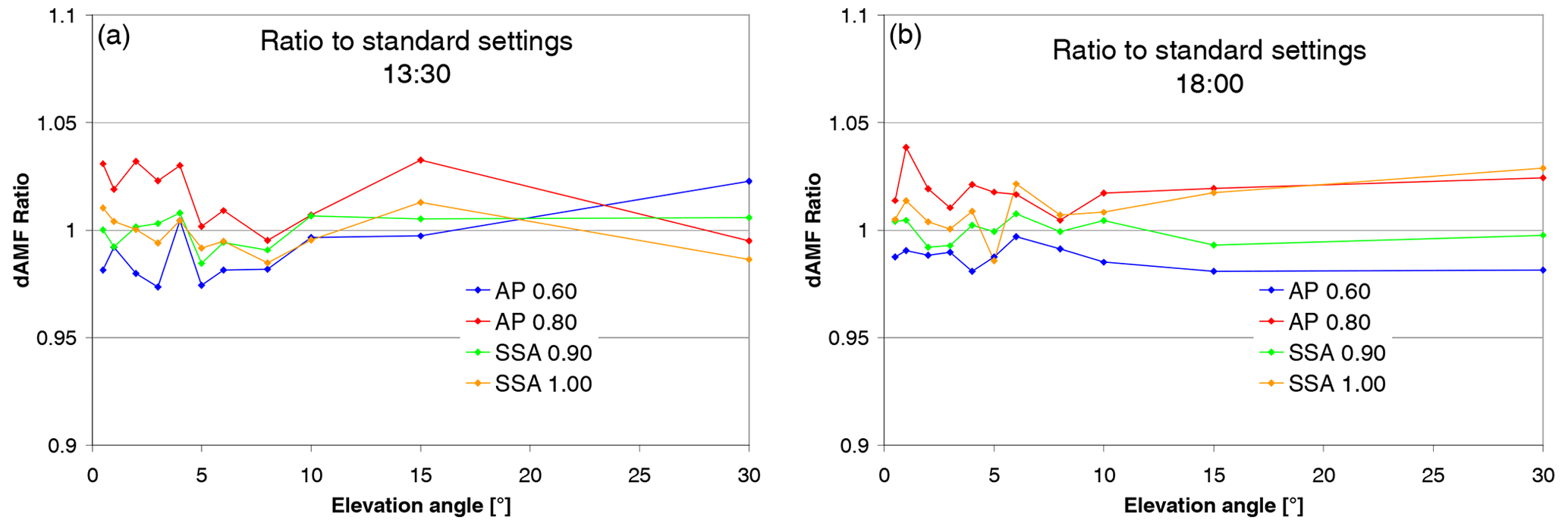
Figure A8 Effect of different phase functions and single scattering albedos on the O₄ dSCDs. Shown are the ratios for simulations with variations of asymmetry parameter (AP) and single scattering albedo (SSA) versus simulations using the standard settings (AP: 0.68, SSA: 0.95). The results are for SZA of 33.6^∘ and RAA of 0.7^∘ (left, around 13:30 UTC) and SZA of 64.5^∘ and RAA of 87.7^∘ (right, around 18:00 UTC) on 2 May 2019. The results for other SZA–RAA combinations during the afternoon of 2 May 2019 are similar.

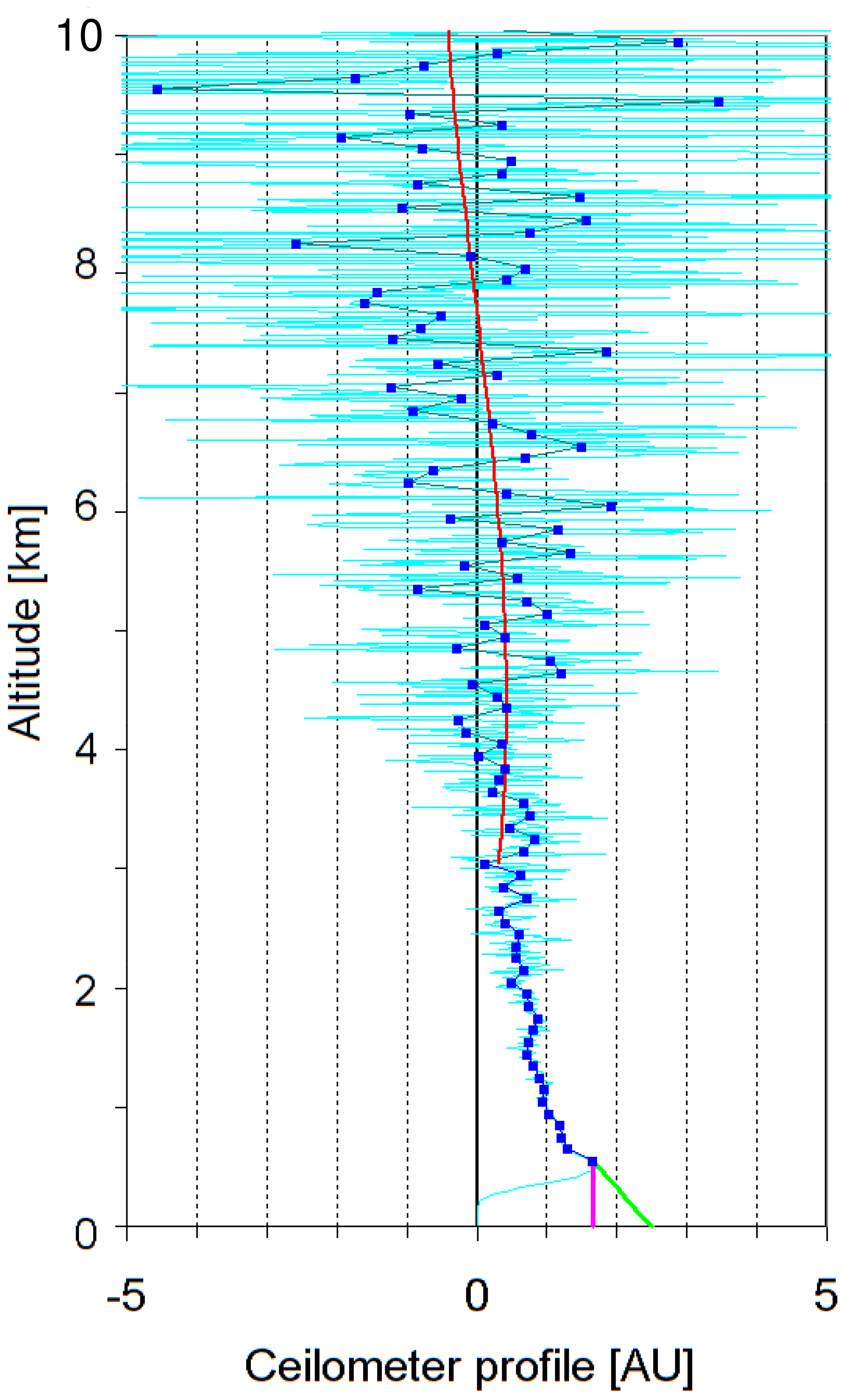
Figure A9 The light blue data show the original backscatter profile averaged between 14:00 and 15:00 UTC. The blue dots show the smoothed (with a 100 m kernel) profile, which are used between 500 m and 3 km. Below 500 m, either constant or linearly extrapolated data (see text) are used. Between 3 and 10 km, a third-order polynomial is fitted to the raw data. The polynomial values are used between 3 km and the altitude at which they become negative. Above, the values are set to zero.

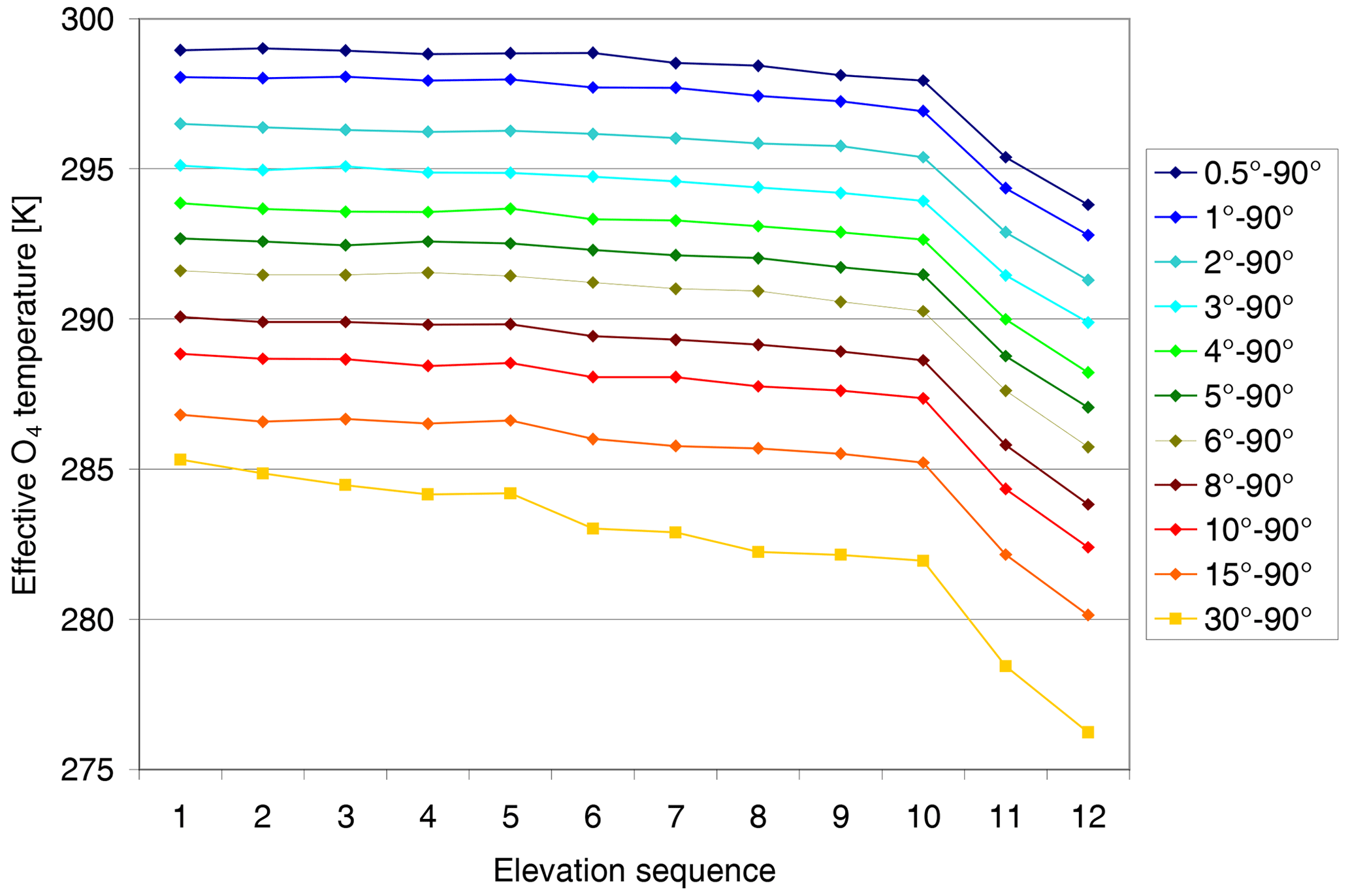
Figure A10 Effective temperatures calculated for the individual measurements according to Eq. (2).

Figure A11 Effect of the temperature correction for two selected elevation sequences.

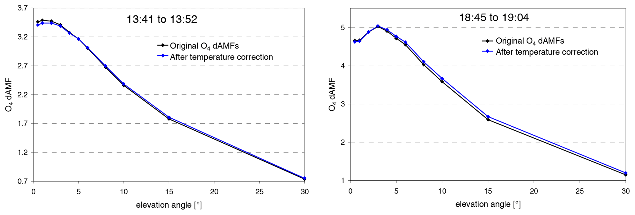
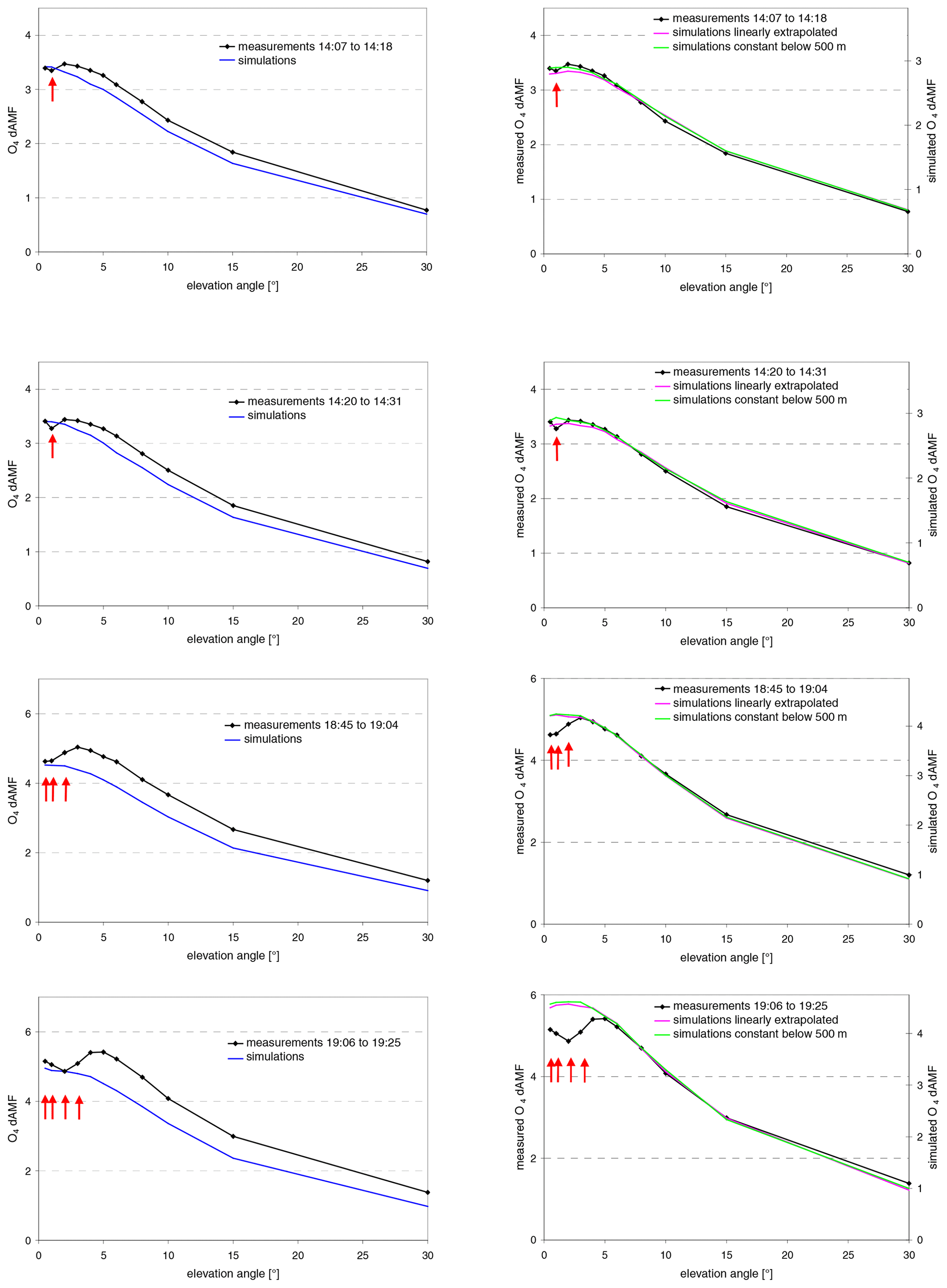
Figure A12 Comparison of the measured and simulated O₄ dAMFs for five elevation sequences with few cloud-contaminated measurements (indicated by the red arrows). On the left side, the measured O₄ dAMFs are compared to simulations for a pure Rayleigh atmosphere. On the right side, they are compared to simulation results including aerosols (two profiles with either constant or linearly extrapolated aerosol extinction below 500 m). Note that on the right side, separate y axes on the right sides are used for the simulation results. The maxima of the right y axes are chosen to achieve the best agreement between the measured and simulated O₄ dAMFs (see text). Note that for the last elevation sequence (19:06–19:25 UTC), the AOD used in the forward model has large uncertainties; see Sect. 2.2.

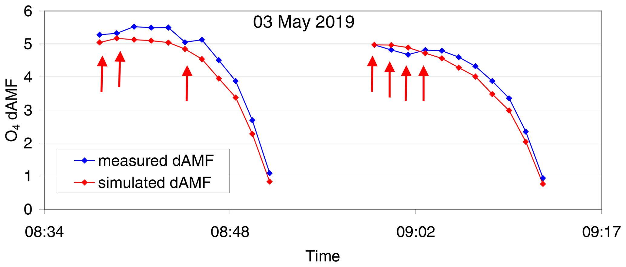
Figure A13 Comparison of the measured and simulated O₄ dAMFs for two elevation sequences on 5 March 2019. For the first elevation sequence, the AOD was < 0.05 at 360 nm. During the second elevation sequence, it already increased to 0.06. The radiative transfer simulations were made for an aerosol-free atmosphere. The red arrows indicate cloud-contaminated measurements.

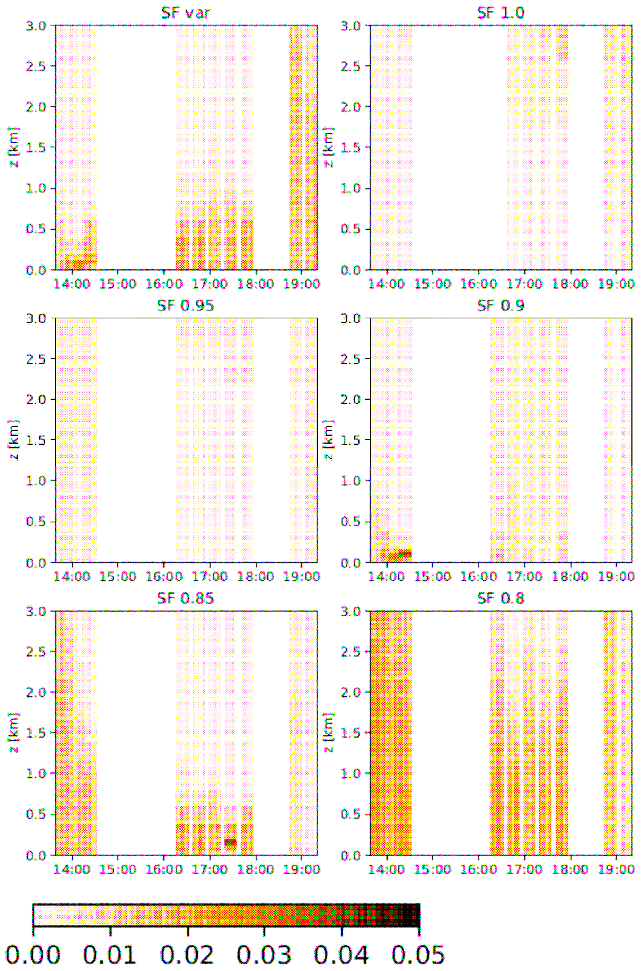
Figure A14 Extinction profiles retrieved with MAPA for the selected elevation sequences for different scaling factors. Only profiles for inversions with “valid” or “warning” flags are shown.

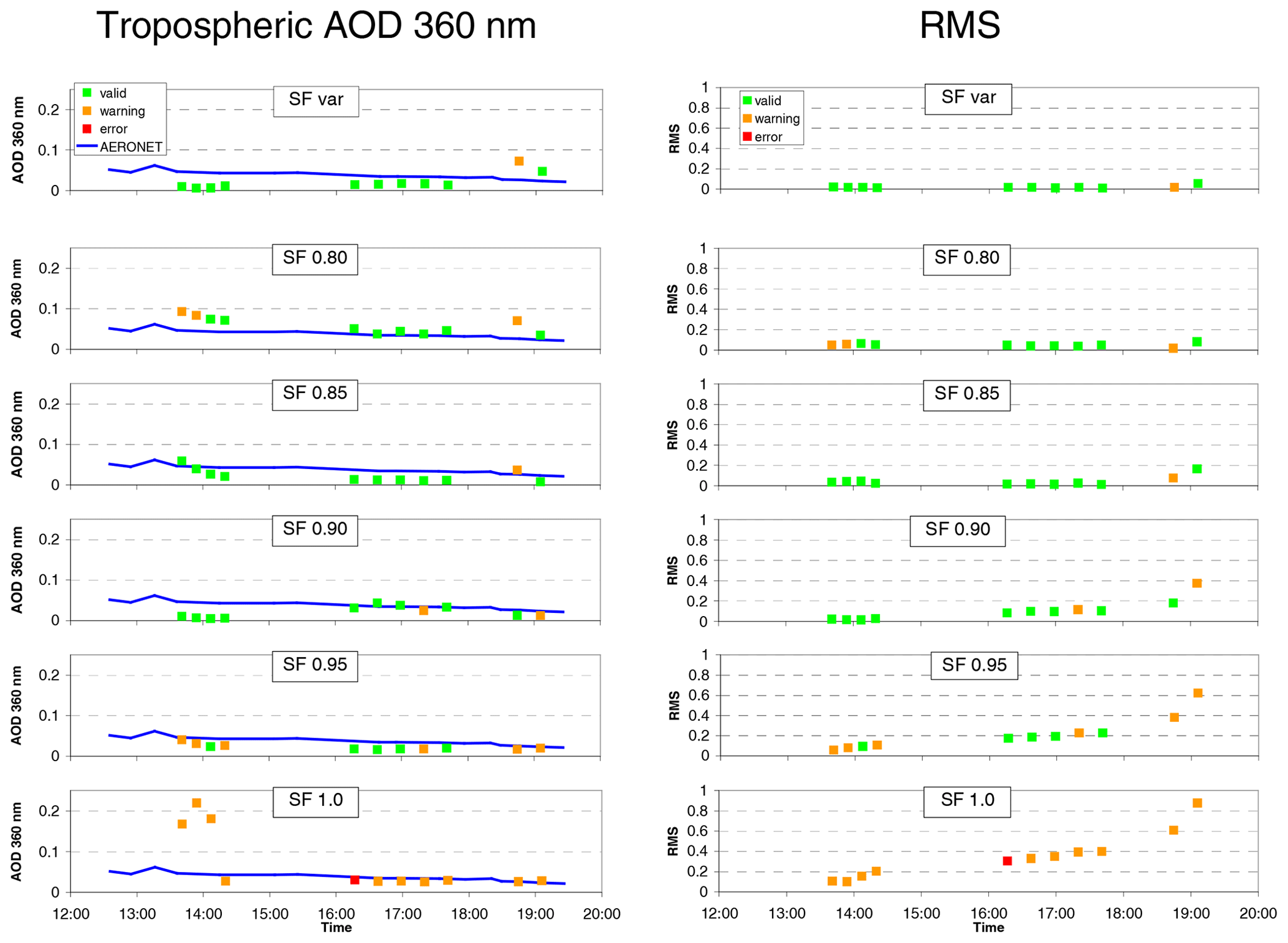
Figure A15 Left comparison of the retrieved AOD for the MAPA profile inversions with different scaling factors (squares) and the (tropospheric) AOD observed by the Sun photometer (blue lines). Right: rms between the measured and fitted O₄ dAMFs. The colours indicate the quality flags for the individual profile inversions.