A local- to national-scale inverse modeling system to assess the potential of spaceborne CO₂ measurements for the monitoring of anthropogenic emissions

This work presents a flux inversion system which assesses the potential of new satellite imagery measurements of atmospheric CO₂ for monitoring anthropogenic emissions at scales ranging from local intense point sources to regional and national scales. Such imagery measurements will be provided by the future Copernicus Anthropogenic Carbon Dioxide Monitoring Mission (CO2M). While the modeling framework retains the complexity of previous studies focused on individual and large cities, this system encompasses a wide range of sources to extend the scope of the analysis. This atmospheric inversion system uses a zoomed configuration of the CHIMERE regional transport model which covers most of western Europe with a 2 km resolution grid over northern France, western Germany and Benelux. For each day of March and May 2016, over the 6 h before a given satellite overpass, the inversion separately controls the hourly budgets of anthropogenic emissions in this area from ∼ 300 cities, power plants and regions. The inversion also controls hourly regional budgets of the natural fluxes. This enables the analysis of results at the local to regional scales for a wide range of sources in terms of emission budget and spatial extent while accounting for the uncertainties associated with natural fluxes and the overlapping of plumes from different sources. The potential of satellite data for monitoring CO₂ fluxes is quantified with posterior uncertainties or uncertainty reductions (URs) from prior inventory-based statistical knowledge.

A first analysis focuses on the hourly to 6 h budgets of the emissions of the Paris urban area and on the sensitivity of the results to different characteristics of the images of vertically integrated CO₂ (XCO₂) corresponding to the spaceborne instrument: the pixel spatial resolution, the precision of the XCO₂ retrievals per pixel and the swath width. This sensitivity analysis provides a correspondence between these parameters and thresholds on the targeted precisions of emission estimates. However, the results indicate a large sensitivity to the wind speed and to the prior flux uncertainties. The analysis is then extended to the large ensemble of point sources, cities and regions in the study domain, with a focus on the inversion system's ability to separately monitor neighboring sources whose atmospheric signatures overlap and are also mixed with those produced by natural fluxes. Results highlight the strong dependence of uncertainty reductions on the emission budgets, on the wind speed and on whether the focus is on point or area sources. With the system hypothesis that the atmospheric transport is perfectly known, the results indicate that the atmospheric signal overlap is not a critical issue. All of the tests are conducted considering clear-sky conditions, and the limitations from cloud cover are ignored. Furthermore, in these tests, the inversion system is perfectly informed about the statistical properties of the various sources of errors that are accounted for, and systematic errors in the XCO₂ retrievals are ignored; thus, the scores of URs are assumed to be optimistic. For the emissions within the 6 h before a satellite overpass, URs of more than 50 % can only be achieved for power plants and cities whose annual emissions are more than ∼ 2 MtC yr⁻¹. For regional budgets encompassing more diffuse emissions, this threshold increases up to ∼ 10 MtC yr⁻¹. The results therefore suggest an imbalance in the monitoring capabilities of the satellite XCO₂ spectro-imagery towards high and dense sources.

1 Introduction

Comprehensive information about anthropogenic CO₂ emissions integrated at the scale of power plants, cities, regions and countries up to the globe would allow decision makers to track the effectiveness of emission reduction policies in the context of the Paris Agreement on climate and other voluntary emission reduction efforts. By observing the CO₂ plumes downwind of large cities and industrial plants as well as atmospheric signals at a few to several hundred kilometer scales, future high-resolution spectro-imagery of the column-average CO₂ dry air mole fraction (XCO₂) from space may help address this need (Ciais et al., 2015; Pillai et al., 2016; Pinty et al., 2017; Schwandner et al., 2017; Broquet et al., 2018). The Copernicus Anthropogenic Carbon Dioxide Monitoring mission (CO2M; Pinty et al., 2017) is a prominent example of such a strategy. The CO2M concept relies on a constellation of sun-synchronous satellites with XCO₂ spectral imagers to be deployed from 2025 by the European Commission and the European Space Agency (ESA). It will be based on passive radiance measurements in the shortwave infrared (SWIR), a part of the spectrum that is sensitive to CO₂ and CH₄ concentrations throughout the troposphere including the boundary layer, like almost all of the space missions that have been dedicated to greenhouse gas (GHG) monitoring so far (Crisp, 2018).

Much remains to be understood and to be developed in order to ensure that such a constellation provides information about emissions with enough detail to be relevant for policy makers. In this context, observing system simulation experiments (OSSEs) of atmospheric inversions with synthetic images of XCO₂ data have supported the design of the space missions that will monitor the anthropogenic emissions (Buchwitz et al., 2013b; Pillai et al., 2016; Broquet et al., 2018). So far, they have mainly focused on plume inversions for some large plants and cities. However, Wang et al. (2019) estimated that cities and plants emitting more than 10 MtC yr⁻¹, like Berlin (in the study by Pillai et al., 2016) and Paris (in the study by Broquet et al., 2018), represent less than ∼ 7 % of the global CO₂ emissions. Furthermore, the studied cases are generally quite isolated from other large CO₂ sources, facilitating the distinction of their plumes in the XCO₂ images, while plumes from neighboring sources could overlap and hamper the attribution to the targeted city or plant. Finally, the signature of emissions in spaceborne imagery does not consist only of clear plumes from cities, industrial clusters and point sources. Despite the large atmospheric signature of the natural fluxes, atmospheric inversions may have the potential to exploit other spatial variations in XCO₂ fields to quantify regional to national budgets of more diffuse sources or of all types of sources, even when the overlapping of several plumes prevents the quantification of the emissions from individual cities and point sources. Therefore, there is a need to extend the OSSEs to a representative range of sources with various emission budgets and spreads, and various distances to other major sources, and to a larger range of spatial scales.

We have developed a high-resolution inversion system for the monitoring of CO₂ anthropogenic emissions at spatial scales ranging from local intense point sources, like industrial sites, to regional and national scales. Furthermore, this system accounts for the uncertainty in the natural fluxes. Our current simulation domain covers most of western Europe with an extensive ensemble of cities, plants and diffuse CO₂ emissions. We use an analytical inversion methodology, which is the most adapted approach to efficiently test a large number of observation scenarios (Sect. 2.1.2), a high-resolution atmospheric transport model (Sect. 2.1.1) and a high spatial resolution distribution of the emissions derived from different inventory products developed by the Institut für Energiewirtschaft und Rationelle energieanwendung (IER) of the University of Stuttgart (Sect. 2.2).

The analytical inversion system follows the traditional Bayesian formalism of the atmospheric inversion. Of direct relevance here, it derives uncertainty statistics of its “posterior” emission estimates for the controlled sources (plants, cities, countryside areas or whole regions) from (i) the assumed uncertainties in the budgets derived from “prior” emission inventories (built on statistics of fossil fuel consumption, activity data and emission factors), (ii) the spaceborne XCO₂ observation sampling and precision and (iii) its atmospheric transport model. The improvement of the knowledge on the emissions enabled by the satellite imagery is quantified here in terms of “uncertainty reduction”, i.e., of the relative difference between the prior and posterior uncertainties.

The inversion system solves for hourly budgets of the emissions from the different types of sources over the 6 h before the satellite observation of the corresponding area. Indeed, Broquet et al. (2018) showed that, due to atmospheric diffusion, the atmospheric signatures of emissions from a megacity like Paris that are detectable in satellite XCO₂ images (made with current measurement capabilities) approximately correspond to the city emissions occurring within less than 6 h before the satellite overpass. This duration should be even shorter for the range of sources analyzed in our study as most of them have lower emissions than Paris. The analysis of the results will primarily focus on the 6 h budgets of the emissions before the satellite observation. However, controlling the hourly budgets allows for the evaluation of the capability to solve for the temporal profiles of the emissions. It also allows for some level of independence between uncertainties in the emissions from different hours to be considered, which limits the ability to cross and extrapolate information throughout the 6 h windows. This point is critical for cities whose detectable atmospheric signatures are representative of emissions on durations shorter than 6 h and, thus, for which there is no direct constraint from the satellite observation in the first hours of such 6 h windows.

The OSSEs presented in this study use a rather simple simulation of the XCO₂ observation sampling and errors from a single helio-synchronous satellite over the area of interest. The aim is indeed to provide a general understanding of the performance of the inversion system and of its potential for monitoring anthropogenic emissions with spaceborne XCO₂ imagery rather than to evaluate a precise mission configuration with precise orbital parameters and instrumental specifications. In terms of errors in the XCO₂ data, the analysis focuses on random errors due to the instrumental noise that have no spatial correlations (even though the topic is explored in Appendix A). Nevertheless, a large range of values for the precision (assumed to be homogeneous in the satellite field of view), horizontal resolution and swath of the spaceborne instrument are tested to assess the impact of these parameters on the inversion results, which can potentially support the design of future missions (Sect. 3.2).

Furthermore, in order to get a wide range of atmospheric transport conditions (in particular of average wind speeds; Broquet et al., 2018) and natural flux conditions (Pillai et al., 2016), inversions are performed for each day of March and May 2016. We work with full images of the plumes from the targeted sources each day by flying a satellite with a large swath in their vicinity on any given day. Partial images of the plumes will be analyzed when studying the sensitivity to the swath width (over Paris) only. The cloud cover and large aerosol loads as well as the corresponding gaps in the spaceborne passive XCO₂ sampling are ignored. In any case, the satellite crosses the area of interest at 11:00 LT (local time) similar to what is currently recommended for the CO2M mission (Pinty et al., 2017), so that the inversion controls the hourly emissions of the sources between 05:00 and 11:00 LT.

The inversion system and the corresponding transport model extend from southern France to northern Germany and from the western UK to eastern Germany (Fig. 1). However, the grid of the transport model is zoomed, and the analysis focuses on a 2 km resolution subdomain covering the north of France (in particular Paris), southeast England (in particular London), west Germany, Belgium, Luxembourg and the Netherlands.

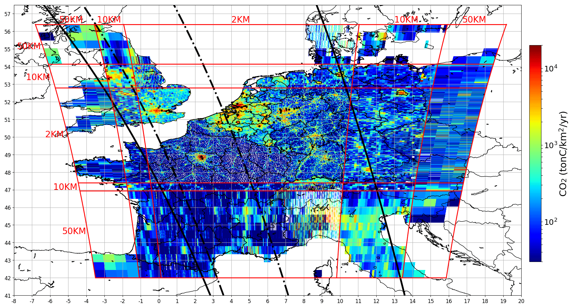
Figure 1 Maps of the IER annual emissions interpolated over the domain of the CHIMERE model. Point sources are indicated by black dots, and administrative regions are shown using thin black lines. The grid of the model is defined by subdomains with several resolutions (r × s km², where r and s are 2, 10 or 50 km), and their boundaries are represented by the red lines. The thick black lines depict the edges of the satellite tracks corresponding to the synthetic data used in this study (300 km swath: dash-dotted line; 900 km swath: solid line).

The first part of the analysis concerns the monitoring of the emissions of Paris and its suburbs, which represent the most populated and densest urban area in Europe. Broquet et al. (2018) chose this megacity as a study case because its emissions are high (∼ 11–14 MtC yr⁻¹ for 2013 according to the AIRPARIF inventory; Staufer et al., 2016; AIRPARIF, 2013), concentrated and relatively distant from other major sources. Moreover, the topography of the region is relatively flat, and the average wind speed is moderate: 7 m s⁻¹ at 100 m above ground level (Broquet et al., 2018). The XCO₂ plume generated by the Paris emissions has a relatively simple structure that often emerges well from the background. Therefore, the monitoring of the emissions of Paris constitutes a very favorable case with respect to other cities in Europe. Broquet et al. (2018) performed some analysis of the sensitivities of the inversion results to the wind speed and to the XCO₂ spaceborne spectro-imagery average precision and horizontal resolution. However, they tested a limited number of values for these observation parameters, in particular few high precisions (<2 ppm) and a single high spatial resolution value (<4×4 km²), while the refinement of the specification of new missions requires an understanding of the sensitivity to choices of precision at the 0.1 ppm scale and to choices of resolution at the 1 km² scale. Indeed, these choices have large impacts on the design of the instrument and, therefore, on its cost (Pinty et al., 2017). Furthermore, Broquet et al. (2018) performed all of their OSSEs with an unique hypothesis on the prior uncertainties in the 1 to 6 h budgets of the emissions from Paris, while acknowledging that the specification of these prior uncertainties could have a significant impact on the results and that the uncertainties in the inventories at such a temporal scale are difficult to assess. Therefore, this study performs a deeper investigation of the sensitivity to the observation precision and spatial resolution, to the wind speed and to the characterization of the uncertainties in the prior estimate of the emissions (Sect. 3.2).

The second part of this study considers the full ensemble of sources, from point sources to regions, in the 2 km resolution subdomain. This subdomain encompasses the Netherlands, Belgium and western Germany; these regions are characterized by densely populated areas distributed over a network of medium-sized towns and by a large number of strong point sources, with, for example, some power plants in western Germany emitting more than 5 MtC yr⁻¹. Thus, the ability of the inversion system to disentangle the plumes from neighboring sources is challenged in these areas.

This paper is organized as follows: Sect. 2 details the theoretical and practical framework of both the inversion system and the OSSEs conducted in this study. Section 3 analyses the results relative to the monitoring of the emissions of Paris and, in particular, the corresponding sensitivity tests (Sect. 3.2). This section also diagnoses the potential of the inversion system with respect to monitoring the anthropogenic emissions at the point source, city and regional scales in the area where flux and concentrations are simulated at a 2 km resolution (Sect. 3.3). Section 4 addresses the robustness and extent of the conclusions that can be derived from this study and proposes some perspectives regarding the analytical inversion system and the monitoring of anthropogenic emissions based on satellite data.

2 Inverse modeling system and OSSEs

In the following sections, we describe the different structural elements of the analytical inversion system: the gridded inventories used to define the point or area sources to be controlled and to map their emissions (Sect. 2.2), the simulation of the atmospheric CO₂ and XCO₂ signatures of the controlled sources using the CHIMERE atmospheric transport model, and the matrix computation of the posterior uncertainties in the emissions (Sect. 2.1.1 and 2.3). We also describe the observations and parameters chosen for the OSSEs in this study: the XCO₂ observation sampling and errors (Sect. 2.1.2) and the prior uncertainties in the emissions, natural fluxes and boundary conditions (Sect. 2.4). New OSSEs with the analytical inversion system can easily be conducted with other options for these observations and parameters. However, for the sake of clarity, the descriptions of the components of the inversion system and of the options for the OSSEs are intertwined.

2.1 XCO₂: transport model simulations and pseudo-data

2.1.1 Simulations of CO₂ and XCO₂ with the CHIMERE model

To compute the 4D CO₂ signatures of surface CO₂ fluxes in the study domain for March and May 2016 as well as of the domain CO₂ boundary conditions, we use the CHIMERE regional atmospheric transport model (Menut et al., 2013). This Eulerian mesoscale model was designed to simulate pollution (Pison et al., 2007) but has also been used for CO₂ atmospheric inversions and, in particular, for city-scale inversions of the emissions from Paris (Bréon et al., 2015; Staufer et al., 2016; Broquet et al., 2018). It has shown high skill in simulating the daily and synoptic variability in the atmospheric CO₂ concentrations at European CO₂ continuous measurement sites (Patra et al., 2008).

The domain of our CHIMERE configuration covers most of western Europe (Fig. 1) between the latitudes ∼ 42^∘ N (northern Spain) and ∼ 56^∘ N (northern Germany) and between the longitudes 6^∘ W (eastern Ireland) and ∼ 17^∘ E (eastern Germany). The horizontal resolution of the zoomed grid of this configuration ranges from 2 to 50 km, with the 2 km × 2 km resolution subdomain being appropriate to simulate the atmospheric signature of a dense network of sources in northern France, Belgium, the Netherlands, Luxembourg and western Germany. The zoom and extent of the CHIMERE grid link the simulation of CO₂ at local scales in this area of interest with the transport of CO₂ at the European scale while mitigating the computational cost. The model has 29 sigma vertical layers that extend from the surface to 300 hPa. Model concentration outputs are averaged at the hourly scale. The meteorological forcing is from the 9 km × 9 km and 3 h resolution analysis of the European Center for Medium-Range Weather Forecasts (ECMWF). These 3-hourly fields are interpolated at the spatial and temporal resolution of CHIMERE. The CO₂ concentrations used to impose the conditions at the initial time and at the lateral and top boundaries of the CHIMERE domain are from the analysis of the Copernicus Atmosphere Monitoring System (CAMS; Inness et al., 2019) at ∼ 16 km resolution. The products used to impose surface CO₂ fluxes in the model are detailed below in Sect. 2.2.

XCO₂ observations and the corresponding signatures of fluxes are simulated from the CO₂ 3D fields from CHIMERE at 11:00 LT. For the sake of simplicity in the OSSEs conducted here, as we use synthetic data only and a rather simple modeling of the spaceborne observation, the computation of XCO₂ assumes that the vertical weighting function of the CO₂ column-averaging (kernel) is vertically uniform. For a given model pixel at latitude “lat” and longitude “long”, XCO₂ is thus computed from the vertical average of the CO₂ mole fractions simulated by the model:

$$\begin{array}{}\text{(1)}& \begin{array}{rl}& {\mathrm{XCO}}_{\mathrm{2}}\left(\mathrm{lat},\mathrm{long}\right)=\\ & {\displaystyle \frac{{\int }_{P_{\mathrm{top}}}^{P_{\mathrm{surf}}}{\mathrm{CO}}_{\mathrm{2}}\left(\mathrm{lat},\mathrm{long},P\right)\mathrm{d}P+\stackrel{\mathrm{‾}}{{\mathrm{CO}}_{\mathrm{2}}}\left(P_{\mathrm{top}}\right)P_{\mathrm{top}}}{P_{\mathrm{surf}}(\mathrm{lat},\mathrm{long})}},\end{array}\end{array}$$

where P designates the atmospheric pressure, P_surf is the atmospheric surface pressure and P_top (300 hPa) is the pressure at the top boundary of the model. For pressures lower than P_top, we assume that the CO₂ concentrations equal the horizontal average of the top-level mixing ratios in CHIMERE $\left(\stackrel{\mathrm{‾}}{{\mathrm{CO}}_{\mathrm{2}}}\right(P_{\mathrm{top}}\left)\right)$. Indeed, we do not expect significant spatial gradients of CO₂ over the simulation domain in the upper atmosphere. This is supported by the lack of signal in our simulations of the atmospheric signatures of the surface fluxes in the upper layer of the model.

2.1.2 XCO₂ pseudo-data sampling and error

As detailed in Sect. 2.3, the OSSE framework of the inversions requires the location and time of the individual XCO₂ data, and the associated error statistics, but not the explicit values of the synthetic observations themselves. In this study, we consider pseudo-satellites with a low Earth orbit (LEO) whose altitude and inclination parameters are similar to those of the A-Train (705 km and 98.2^∘, respectively; Parkinson et al., 2006). The satellite observations are assumed to occur at 11:00 LT in the morning. Successive tracks of a single satellite on this orbit are separated by ∼ 25^∘. However, we do not study the potential of a specific satellite nor that of a constellation of such LEO satellites depending on their number. Furthermore, this study focuses on results at the scale of 6 h. Therefore, for any day, it considers single satellite tracks that do not correspond to a specific position of a satellite on the chosen orbit: when studying the emissions of the Paris urban area, we use the track that is nearly centered on this city every day, and various swaths are considered to study the sensitivity of the results to this parameter (Sect. 3.2.2). For the study of results for the ensemble of sources contained within the 2 km subdomain (Sect. 3.3), we use a track centered over Belgium every day and a 900 km swath to ensure a full coverage of the plumes from these sources (the sensitivity to a realistic range of swath widths is not investigated in this second set of analyses).

Our OSSEs assess the impact on the inversion results of the measurement noise from the satellite instrument only, ignoring the errors associated with the radiative transfer inverse modeling for the retrieval of the XCO₂ data from the radiance measurements (Buchwitz et al., 2013a; Broquet et al., 2018), in particular any “systematic error”. Thus, the errors on the XCO₂ data at the spatial resolution of the measurements are assumed to be Gaussian, unbiased and uncorrelated in space or time. The distribution of the standard deviation (SD) for these errors is also assumed to be uniform; therefore, these errors are summarized by a single value of SD (denoted as the data precision hereafter).

A large number of scenarios are tested for the observation specifications: the precision on the individual XCO₂ data varies between 0.3 and 2 ppm, and the spatial resolution of the ground pixels can take the following values: 2 km × 2 km (longitude × latitude), 2 km × 3 km, 3 km × 3 km, 3 km × 4 km and 4 km × 4 km. The reference is a precision of 0.6 ppm and a spatial resolution of 2 × 2 km². These values are similar to the characteristics of the simulation of CO2M data used in the study of Wang et al. (2020). When studying the sensitivity of the results over Paris to the swath of the instrument, the swath is varied from 100 to 600 km, with a reference value of 300 km.

2.2 CO₂ fluxes

2.2.1 Maps and time series of anthropogenic emissions and natural fluxes

High-resolution maps of anthropogenic emissions are needed to define appropriate point and area sources to be controlled by the inversion. High-resolution maps of anthropogenic and biogenic fluxes are also needed to distribute the controlled local to regional budgets of these fluxes on the spatial grid of the CHIMERE model. Finally, such maps are needed to provide insights into the typical budgets of fluxes at the control resolution and, thus, to quantify the prior uncertainty in these budgets with a suitable order of magnitude.

The anthropogenic CO₂ emissions are extracted from several datasets compiled by IER (Pregger et al., 2007; Thiruchittampalam et al., 2012). These datasets provide maps of the annual budgets per sector of anthropogenic activity over different domains and at different spatial resolutions. We have merged and re-gridded them to derive a map of the annual budgets of emissions over the entire grid of the CHIMERE configuration. The emissions corresponding to France and Germany are extracted from the respective IER national maps for 2005 at a 1 min resolution, whereas emissions in Belgium, Luxembourg and the Netherlands are derived from an IER 1 km product covering northern Europe for 2005. The IER 5 km resolution map covering the whole of Europe for 2008 is used for the emissions over the rest of the domain. The gridded area sources in the IER maps are interpolated on the CHIMERE grid, but the large point sources are relocated as point sources in individual CHIMERE grid cells. We then derive the hourly emission maps from the annual emission map by applying the convolution of IER typical temporal profiles specific to each country and sector. These profiles include seasonal, daily and diurnal variations of emissions for large sectors such as traffic, power demand, domestic heating or air-conditioning (Pregger et al., 2007).

The IER maps for France, Germany, northern Europe and the whole of Europe correspond to annual budgets for years (2005 and 2008) that can be different from one area to another and that are different from the year chosen for the atmospheric transport and for the natural fluxes (2016). This could raise some inconsistencies if assimilating real data into the inversion. However, this study is based on OSSEs with some strong simplifications regarding the observation system, as the overarching target is a general understanding of the behavior and potential of the inversion. This requires the use of a high-resolution and realistic distribution of the emissions in space and time but not a precise estimate of their amplitudes for a given year.

The land surface natural fluxes are derived from 8 km resolution simulations made with the Vegetation Photosynthesis and Respiration Model (VPRM) for the year 2016. This prognostic model delivers hourly values of net ecosystem exchange (NEE) by assimilating satellite and meteorological data (Mahadevan et al., 2008). These values of NEE are interpolated over the CHIMERE area at the hourly timescale. Natural ocean fluxes are ignored.

2.2.2 Controlled areas

The resulting hourly maps of anthropogenic CO₂ emissions for spread sources and large point sources are decomposed spatially to define the areas for which hourly emission budgets are controlled by the inversion: large point sources, cities, remaining parts of regions from which point sources and cities have been extracted (covering diffuse emissions only), and full regions where point sources and cities are not controlled separately but are combined with diffuse emissions. Hourly budgets of the natural fluxes are controlled for full regions only, with the regions used for the control of anthropogenic and biogenic fluxes being identical.

The definition of the regions is done considering the whole domain. It corresponds to administrative regions of France, Belgium, the Netherlands, Luxembourg and Germany, and to three additional large “regions”: the UK, Switzerland and the rest of the domain. This subdivision results in 67 regions (Fig. 1). These 67 regions correspond to the spatial resolution of the natural fluxes in the inversion.

Point sources and cities are controlled individually in the 2 km resolution part of the CHIMERE grid only (Sect. 2.1.1; Fig. 1). In the 39 regions entirely comprised within this subdomain, we individually control the 84 point sources (e.g., factories, power plants) whose annual emissions are larger than 0.2 MtC yr⁻¹. The maps of the remaining emissions (excluding these point sources) in each of these 39 regions are then processed to extract large urban areas to be controlled independently, ensuring at least one controlled urban area per region, and that no controlled urban area overlaps two different regions. An algorithm of pattern recognition has been designed for such an extraction, with the idea that urban areas correspond to clusters of adjacent high-emitting pixels (also followed by Wang et al., 2019). After having applied a Gaussian filter to smooth the spatial distribution of the emissions, the large urban areas are defined by a label-connecting algorithm (Stockman et al., 2001) that identifies the clusters of adjacent points whose emissions are above a predefined threshold. As the density and extension of cities vary considerably amongst the different regions, the parameters of the pattern recognition algorithm, i.e., the standard deviation of the Gaussian filtering and the emission threshold, are different for each region to ensure that each region contains at least one controlled urban area (Fig. 2). As a result, we identify 152 controlled urban areas within the 2 km resolution subdomain. They are characterized by a wide range of budgets and spatial spread of their emissions, their annual budgets range between ∼ 0.07 and ∼ 9.9 MtC yr⁻¹ (with a mean and a standard deviation of ∼ 0.8 and ∼ 1.5 MtC yr⁻¹, respectively), and their areas range from ∼ 8 to ∼ 2400 km² (with a median value of ∼ 240 km²).

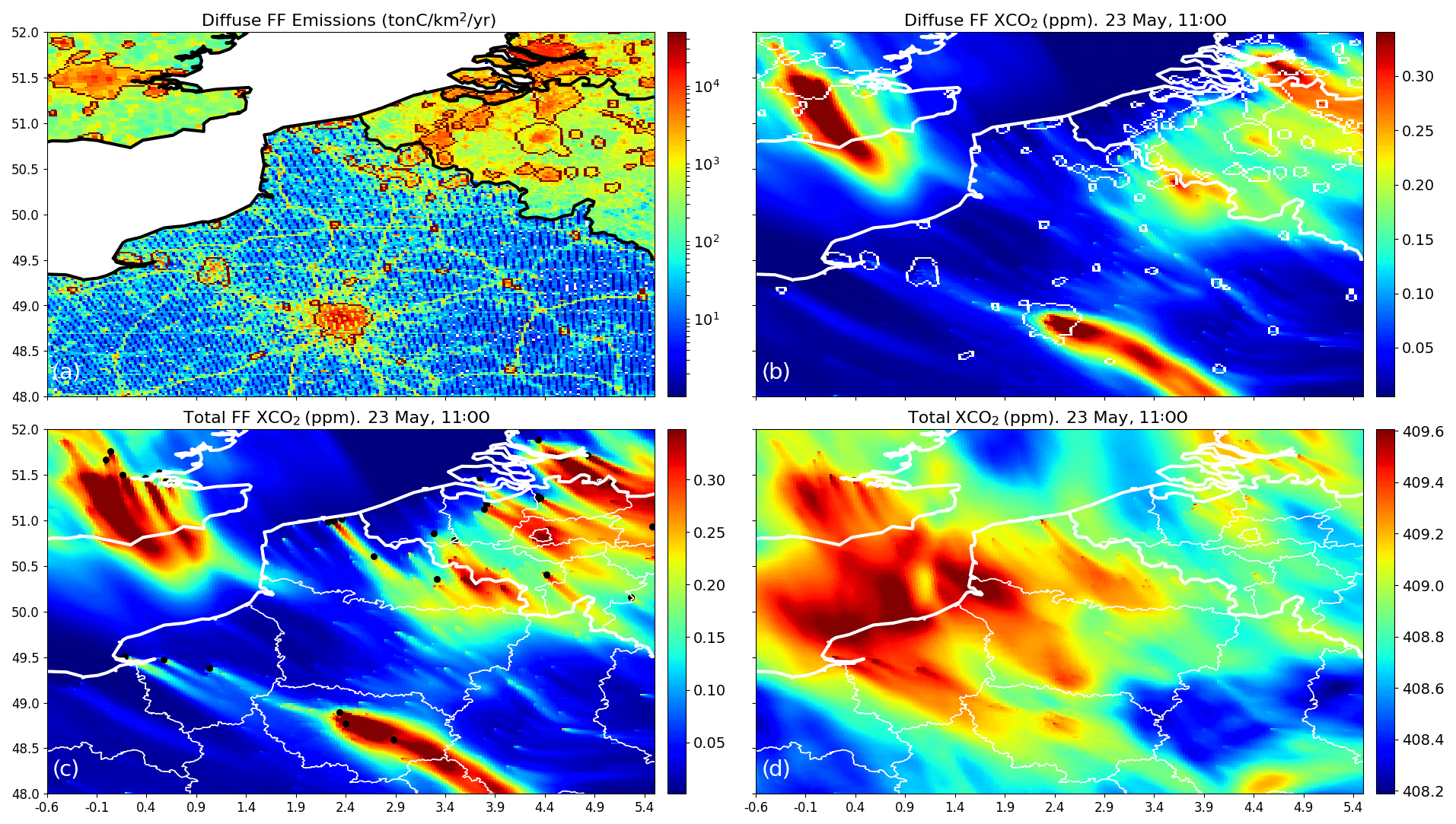
Figure 2 IER emission maps interpolated over northern France, western Belgium and the London area (a). We have represented the anthropogenic emission sources without point sources (“area emissions”). Red curves depict the boundaries of the city clusters defined by a pattern recognition algorithm (Sect. 2.2.3). Panel (b) shows the simulations of XCO₂ (ppm) that are produced by the area emissions. Panel (c) shows the simulations of XCO₂ (ppm) that are produced by the total anthropogenic emissions. Panel (d) shows simulations of XCO₂ (ppm) on 23 May at 11:00 LT that are produced by the combined anthropogenic, natural and boundary fluxes between 05:00 and 11:00 LT. For the sake of clarity, these figures do not show the whole 2 km resolution subdomain of CHIMERE; instead, they illustrate the patterns seen over this subdomain.

The remaining emissions, after having extracted the large point sources and urban areas in the 39 regions, are considered to be diffuse and are hereafter referred to as the “countryside” emissions. The inversion controls their budgets in each region. The analysis of the results at the regional scale for these 39 regions will consider either the countryside emissions only (i.e., focusing on the individual control variables) or their aggregation with the emissions from the point sources and cities within the same region (i.e., considering the full geographical extent of the regions). The inversion also directly controls the total budget of the emissions for the 28 regions that are not fully comprised in the 2 km subdomain (most of these 28 regions do not overlap this subdomain at all). Overall, the control of countryside or total regional emissions adds 67 controlled areas (corresponding to the 67 regions) for the anthropogenic emissions so that the inversion controls the hourly budgets of anthropogenic emissions for 303 areas (84 point sources, 152 urban areas and 67 countryside or regional areas) and the hourly budgets of natural fluxes for 67 areas.

2.3 Analytical flux inversion

2.3.1 Theoretical framework

The inversion system follows a traditional analytical inversion approach based on the Bayesian formalism and assuming that error statistics follow Gaussian distributions (Tarantola et al., 1987; Broquet et al., 2018). The system controls factors that scale the hourly budgets of the different control areas for the anthropogenic and biogenic fluxes defined in Sect. 2.2.2. It also controls a single scaling factor applied to the CO₂ field used to impose the initial, lateral and top CO₂ boundary conditions of the model, as such boundary conditions generally bear important large-scale uncertainties that can impact the estimates of sources within the domain (Broquet et al., 2018). In the OSSEs of this study, the inversion periods for each day in March or May 2016 cover the 6 h (05:00–11:00 LT) before 11:00 LT, when the satellite observations are supposed to be made. The number of control variables (2221=370 controlled areas × 6 time slots + 1 control variable for the boundary conditions) is sufficiently small to solve the inverse problem analytically. However, building the matrix H that encompasses the atmospheric transport operator and that is described below (Sect. 2.3.2) requires a large computational burden.

For a given inversion period, we define the control vector x as the set of controlled scaling factors for the hourly flux budgets and the boundary conditions. The prior uncertainty in x is assumed to follow a Gaussian distribution and to be unbiased. Thus, it is characterized by the uncertainty covariance matrix B.

In this study, the observation vector y is defined by the XCO₂ concentrations in the transport model horizontal grid cells sampled by the observations. The simulation of y based on a given estimate of x is given by the linear observation operator H: $\mathit{x}\to \mathit{y}=\mathbf{H}\mathit{x}$, which chains three operators. The first operator H_distr distributes the controlled hourly budgets of emissions in space within the controlled areas and provides the spatial and temporal mapping of the boundary conditions whose scaling factor is controlled by the inversion. The second operator H_transp is the atmospheric transport from the emissions and the boundary conditions to the full CO₂ and XCO₂ fields. Finally, the third operator H_sample performs the XCO₂ sampling at the location of the XCO₂ data (Sect. 2.1.2). Differences between Hx and observed values for y arise due to (1) uncertainties in x and (2) the combination of errors in the observation operator and in the observation data that are together referred to as “observation errors”. The errors from the observation operator are strongly associated with the atmospheric transport model errors (Houweling et al., 2010; Chevallier et al., 2010) as well as with the discretization and spatial resolution of the transport and inversion problems, which raise representation and aggregation errors (Kaminski et al., 2001; Bocquet et al., 2011). Assuming that they follow Gaussian and unbiased distributions like the prior uncertainties, these observation errors are fully characterized by the observation error covariance matrix R. The H, B and R matrices must be explicitly estimated in the analytical inversion framework (Sect. 2.3.2 and 2.4).

The Bayesian theory (Tarantola et al., 1987) states that the statistics of the knowledge on x knowing (i) the prior estimate of x, (ii) the observed values for y and (iii) H as a link between the x and y spaces, follow a Gaussian and unbiased distribution. Thus, the uncertainty in such a posterior estimate is fully characterized by the posterior uncertainty covariance matrix A given by

$$\begin{array}{}\text{(2)}& \mathbf{A}={\left[{\mathbf{B}}^{-\mathrm{1}}+{\mathbf{H}}^T{\mathbf{R}}^{-\mathrm{1}}\mathbf{H}\right]}^{-\mathrm{1}}\end{array}$$

The analysis of A and its comparison to B, aggregated or not over different spatial and temporal scales, are the critical diagnostics in this study to assess the potential of inversions assimilating XCO₂ images. The score of uncertainty reduction for a given flux budget is a common indicator for evaluating the performance of an observation system. It is defined as the relative difference between the SD of the prior (σ_prior) and posterior (σ_post) uncertainties in this flux budget ($\mathrm{UR}=\mathrm{1}-\frac{{\mathit{\sigma }}_{\mathrm{post}}}{{\mathit{\sigma }}_{\mathrm{prior}}}$). If the assimilation of satellite observations perfectly constrains a given flux budget, the corresponding UR equals 100 %. If this assimilation does not provide any information on the flux budget, UR equals 0 %.

2.3.2 Building the observation operator matrix H

The analytical inversion system is essentially built on the explicit computation of H = H_distrH_transpH_sample. The different columns of H correspond to the signatures (or “response functions”) in the observation space of the different control variables, i.e., of the different hourly emissions for each control area, and of the boundary conditions. They are computed by applying the sequence of operators H_distr, H_transp and then H_sample to each control variable set to 1, keeping the others null (Broquet et al., 2018). H_distr is defined based on the flux maps detailed in Sect. 2. H_transp corresponds to the CHIMERE model and to the vertical integration of CO₂ into XCO₂ presented in Sect. 2.1.1, while H_sample corresponds to the sampling, on the transport model grid, of the simulated XCO₂ values according to the spatial distribution of the pseudo-observations (Sect. 2.1.2). A generalized H is actually stored for the analytical inversion system to anticipate any option for H_sample, by recording the full CO₂ and XCO₂ fields from the application of H_distrH_transp to each control variable, i.e., the full CO₂ and XCO₂ signatures of each control variable.

2.4 Practical implementation of the OSSEs

While, in principle, R should characterize both the errors in XCO₂ data and the errors from the observation operator H, this study focuses on the impact of the observation sampling and errors only. It ignores the errors from the observation operator. Moreover, the observation errors are restricted to the measurement noise, which is uncorrelated in space and time as detailed in Sect. 2.1.2. Thus, the different R matrices used for the OSSEs (depending on the observation sampling and noise) are all diagonal. The errors on the individual pseudo-observations are described by a uniform precision (${\mathit{\sigma }}_{{\mathrm{XCO}}_{\mathrm{2}}}$) depending on the chosen satellite configuration (Sect. 2.1.2). However, the observation vector y is defined by the transport model grid rather than by the precise location and coverage of the data. Therefore, the diagonal elements of R follow the aggregation of n_obs pseudo-observations with uncorrelated errors (where n_obs is potentially greater than 1) within each model grid cell corresponding to an element of y, so that the resulting SD of the errors for this element is given by $\frac{{\mathit{\sigma }}_{{\mathrm{XCO}}_{\mathrm{2}}}}{\sqrt{n_{\mathrm{obs}}}}$.

Prior estimates of anthropogenic emissions and biogenic fluxes are generally provided by inventories and ecosystem model simulations such as those used here in H_distr to distribute the fluxes at high resolution. B should characterize uncertainties in such products and is thus set with values corresponding to typical relative uncertainties in the budgets from the maps detailed in Sect. 2.2.1. Prior estimates of the boundary conditions for regional inversions are usually interpolated from large-scale analysis or inversions. Such products can bear significant large-scale errors at the boundaries of Europe (Monteil et al., 2020). We reflect this by setting the standard deviation of the prior uncertainty in the scaling factor for the boundary conditions in B (see below). When constructing the B matrices in all of our OSSEs, we assume that there is no correlation between the prior uncertainties associated with different controlled emission areas or between these uncertainties and that associated with the boundary conditions. The spatial correlations of the uncertainties in anthropogenic emission inventories is a complex topic, and the current lack of characterization for such correlations led to such a conservative setup (Wang et al., 2018; Super et al., 2020). However, we model the temporal correlations between prior uncertainties in scaling factors associated with different hourly natural or anthropogenic flux budgets of the same controlled emission area by using an exponentially decaying function with a correlation timescale τ (like, for instance, Bréon et al., 2015):

$$\begin{array}{}\text{(3)}& {\mathit{\rho }}_{i,j}=e^{-\frac{\mathrm{|}j-i\mathrm{|}}{\mathit{\tau }}},\end{array}$$

where j and i are the indices of 2 corresponding hours. The SD of the prior uncertainties in the scaling factors for the different hourly budgets of the same controlled area are fixed to an identical value σ_hour. Finally, we assume that the SD of the prior uncertainties in scaling factors for the 6 h budgets of the natural fluxes or of the anthropogenic emissions from a controlled area from 05:00 to 11:00 LT (to be applied to the budgets from the IER and VPRM products presented in Sect. 2.2.1 and used to build H_distr) is fixed to a value σ_Budget that is the same for all control areas: typically 50 % or 100 % of the 6 h budgets. The SD of the prior uncertainties in the scaling factors for the hourly budgets of the controlled areas σ_hour are then derived based on these different assumptions. The reference parameters for B are fixed to τ=3 h and σ_Budget=50 %. Despite the differences between the temporal variations of the hourly emissions from one control area to another or between natural and anthropogenic fluxes in H_distr, these SD values show a negligible variation of less than 1 %, and when considering the reference setup for B, σ_hour∼65 %. The sensitivity of the inversion to the values of σ_Budget and τ is assessed in Sect. 3.2.3. Finally, we use 1 % for the SD of the prior uncertainty in the scaling factor associated with the boundary conditions (i.e., typically an uncertainty of ∼ 4 ppm in the average boundary conditions). This value is quite pessimistic, but some tests in which this value was varied (not shown) demonstrate a very weak sensitivity of the results for the fluxes to this parameter.

3 Results

3.1 High-resolution simulations of XCO₂

Previous sections documented how, for each 6 h period, the inversion system exploits the simulated XCO₂ fields at 11:00 LT to constrain each hourly budget of the anthropogenic or natural fluxes of the controlled areas between 05:00 and 11:00 LT. The CHIMERE full XCO₂ simulations between 05:00 and 11:00 LT with the anthropogenic emissions, natural fluxes and/or domain boundary conditions detailed in Sect. 2.1 and 2.2 are used in this section to compare the overall signatures of these components and of the controlled areas as well as to discuss their overlapping. Figure 2b shows the XCO₂ signatures of all the anthropogenic emissions in the domain except those from the 84 point sources controlled individually by the inversion in the 2 km resolution subdomain (that are illustrated in Fig. 2a). Figure 2c integrates the XCO₂ produced by the 84 point sources and shows the signature of all the anthropogenic emissions. Finally, Fig. 2d displays the superposition of the XCO₂ signatures of all the anthropogenic emissions, of the natural fluxes and of the boundary conditions. For all of these figures, XCO₂ values are taken at 11:00 LT and are provided by simulations between 05:00 and 11:00 LT on 23 May which is a day of strong northwest wind (∼ 10 m s⁻¹ over Paris at 700 m above ground level).

The strong plumes from the megacities of Paris and London are easily distinguished when considering the signature of anthropogenic emissions in Fig. 2b and c, with their amplitude exceeding 0.3 ppm at 100 km downwind of these cities and with sharp gradients of XCO₂ at their edges. The relative narrowness, extended length and small intensity of the plumes shown in Fig. 2b and c are explained by the magnitude of the wind speed on 23 May. The characteristics of those plumes vary considerably with respect to the wind speed, and the inversion results are strongly impacted by this parameter (Sect. 3.2.1; Broquet et al., 2018).

Figure 2b and c also show that the overlapping of plumes from urban areas in Belgium and in the Netherlands produces XCO₂ patterns whose amplitudes are comparable to those of the plumes from Paris and London. However, due to the urban density of those countries, the level of distinction between the individual signatures of the different cities is weak. If we exclude Paris, northwestern France has a much less dense urban fabric with scattered cities of small extents. This sparse distribution allows the relatively weak plumes from cities to be visible, whereas the more diffuse XCO₂ signatures of the countryside emissions do not form any distinguishable patterns (Fig. 2b).

The comparison between Fig. 2b and c highlights the plumes from some of the large 84 point sources within the 2 km resolution subdomain (Sect. 2.2.2). The amplitude of these plumes can locally reach that of Paris but such an increase above the background occurs on a much smaller extent: for instance, that of the power plant close to Dunkerque (∼ 51^∘ N, ∼ 2.3^∘ E) on the northern French coast reaches 0.4 ppm, but its width does not extend to more than 5 km (Fig. 2c). The capacity of our high-resolution transport model to simulate narrow XCO₂ plumes from point sources or urban areas distinct from that of neighboring or surrounding sources is revealed by the example of several point sources in Belgium as well as that of the oil refinery of Grandpuits (48.59^∘ N, 2.94^∘ E) whose plume stands out of the large plume from the Paris urban area (Fig. 2c). The 2 km resolution zoom of the model grid allows one to distinguish those features that would be blurred in a coarser-resolution transport model.

When including the XCO₂ produced by the natural fluxes and the boundary conditions, identifying the features produced by the anthropogenic emissions is more difficult (Fig. 2d). The atmospheric signatures of Paris, London and the high-emitting power plants are hardly differentiated from patterns produced by the boundary conditions and natural fluxes, even though they are still visible. The isolated plumes of low amplitudes from scattered cities with small extents and low emission budgets can hardly be seen. The boundary conditions and the natural fluxes tend indeed to produce signatures whose amplitude is often larger than, or at least comparable to, that of the signal from the anthropogenic emissions, with which they interfere. This blurs this signal of the anthropogenic emissions, especially when the emissions are diffuse. Boundary conditions and natural fluxes are, however, much more distributed homogeneously than the anthropogenic emissions, which are localized over a small fraction of the surface. As a consequence, the boundary conditions and the natural fluxes produce smooth XCO₂ fields (Fig. 2d), whereas the anthropogenic emissions produce heterogeneous fields with finer structures and sharper gradients (Fig. 2c). Therefore, the separation between the two types of fluxes could rely on the differences in terms of spatial scales of their atmospheric signatures or on a precise knowledge of the atmospheric transport patterns.

This first qualitative overview of the atmospheric signatures could imply that the ability to quantify the budgets of emissions for the two megacities, for most of the 84 large point sources, and for large regions in the northeast should be much larger than for the individual urban areas in most of the domain or for the countryside emissions. However, this diagnostic relies on a qualitative assessment of Fig. 2. In Sect. 3.3, we will quantitatively analyze the inversion results as a function of the type of sources.

3.2 Potential of the satellite images for monitoring the anthropogenic emissions of a megacity: sensitivity studies

This section assesses the performance of our inversion assimilating XCO₂ images to monitor the anthropogenic emissions from the Paris area as a function of the wind conditions; as a function of the XCO₂ observation precision, resolution and swath; and as a function of the configuration of the prior error covariance matrix B. The results are relative to the inversion control area that covers most of the Paris urban area (Fig. 2a). The analysis is based on sixty-two 6 h inversion tests with satellite images nearly centered on this area for each day of March and May 2016. With the reference 300 km wide swath, such images cover the plumes from the Paris urban area entirely under most wind conditions (Broquet et al., 2018). In the following, the wind speed is characterized by its averaged value at 700 m above ground level over the inversion control area corresponding to Paris and over the period corresponding to the chosen diagnostic: over 05:00–11:00 LT when analyzing the uncertainty in the budgets of the emissions corresponding to the full 6 h period of inversion or over the [hh,11:00] time interval when analyzing the uncertainty in the hourly budget of the emissions between the hours hh and hh+1.

3.2.1 Impact of the wind speed

A first set of inversions is conducted with the reference values for the precision, resolution and swath of the satellite observation and for the parameters of the prior uncertainty (0.6 ppm, 2 × 2 km², 300 km, 50 % and 3 h, respectively). These inversions are applied to 12 different days in March 2016 which present a range of average wind speeds from 2 to 14 m s⁻¹ (Fig. 3). We investigate results in winter, when the amplitudes of the biogenic fluxes are low, to mitigate the influence of these fluxes (and of their variability) on the URs for the Paris emissions. Note that the time profiles modeling the variability in the anthropogenic emissions ignore day-to-day variations (except between weekend and working days) which almost removes the influence of the variability in these emissions when studying results in March only. Results are presented in terms of prior and posterior uncertainties in both the 1 and 6 h budgets of emissions from the Paris urban area. The directions of the wind are predominantly meridional so that the selection of the swath has no impact. The main analysis and conclusions in this section are similar to that of Broquet et al. (2018), so we present them briefly.

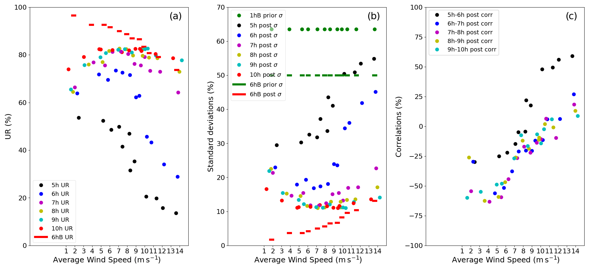
Figure 3 Uncertainty reductions (UR) from a 50 % prior uncertainty on the 6 h budgets of the Paris emissions for 12 d characterized by different average wind speeds over Paris (a). The UR for hourly and 6 h budgets of the Paris emissions are shown using colored dots and red segments, respectively. In panel (b), the prior vs. posterior uncertainties on 1 h emissions (colored dots) and 6 h emissions (green and red segments) of Paris are shown. In panels (a) and (b), the colors of the dots represent the hour of the corresponding 1 h budget; the green dots represent the prior uncertainties on the 1 h emissions (1 hB prior σ) which are derived from 50 % prior errors on the 6 h budgets (6 hB prior σ) and by considering temporal prior correlations of 3 h. Panel (c) shows correlations between posterior uncertainties in two consecutive 1 h emissions (colored dots). Results are computed with a retrieval resolution of 2 km × 2 km, a precision of 0.6 ppm and a swath of 300 km.

Results in Fig. 3 illustrate the fact that higher wind speeds lead to smaller uncertainty reductions for the 6 h emission budgets: on 3 March, the average wind speed is 13.5 m s⁻¹ and the UR with the reference values for the precision, resolution and swath is 74 %; whereas on 10 March, the average wind speed is ∼ 1.8 m s⁻¹ and the UR is 97 % (Fig. 3a). Stronger winds decrease the UR because, due to an increased atmospheric dilution, the amplitude of the city plume is smaller which decreases the signal-to-noise ratio for the inversion. However, when considering the UR for hourly emissions, this rule may not apply for wind speeds lower than 6 m s⁻¹. For this range of wind speeds, the posterior uncertainty in 09:00–10:00 LT and 10:00–11:00 LT emissions increases with decreasing wind speed (Fig. 3b). The inversion system shows difficulties in distinguishing the atmospheric signatures produced by consecutive hourly emissions because these signatures have a significant overlap when the wind speed is low. This explanation is confirmed by the negative correlations found between the uncertainties in consecutive hourly emissions, as the magnitude of these negative correlations increases when the wind speed decreases (Fig. 3c). Important negative correlations also explain that 6 h emission budgets are better constrained for low wind conditions, even though hourly emissions can be poorly constrained. The overestimation of some hourly emissions is compensated for by the underestimation of other hourly emissions.

The uncertainty reductions for 1 h and 6 h budgets are high for a large range of wind values: in all the tests here, the URs for the 6 h budgets are above 74 % and the UR for the 1 h budgets after 07:00 LT are above 62 % (Fig. 3a). Concerning the 1 h budgets of the 05:00 to 07:00 LT emissions, the corresponding URs significantly decrease for wind speeds above 10 m s⁻¹. In particular, the UR for the 5:00 to 6:00 LT emission drops below 20 % above this value for the wind speed. This behavior is consistent with the fact that the signatures of emissions occurring well before the satellite overpass have been much more diffused through atmospheric transport at the observation time than that of later emissions.

3.2.2 Impact of the precision, resolution and swath of the satellite images

Figures 4a–d show the URs for the 6 h emission budgets of 3 March (with strong wind), 10 March (with low wind), 23 May (with strong wind) and 27 May (with low wind). This figure corresponds to a second set of inversions performed with the range of options for satellite data precisions and resolutions presented in Sect. 2.1.2 but with the observation swath, the relative prior uncertainty in the 6 h budgets of fluxes and the correlation length scale for the prior uncertainties in hourly fluxes fixed to the reference values (300 km, 50 % and 3 h, respectively). The sensitivity of the UR to the measurement precision and resolution increases with stronger winds. For example, on 27 May (under weak wind) and 23 May (under strong wind), the UR increases by 16 % and 48 %, respectively, between inversions with 2 ppm precision data and inversions with 0.3 ppm precision data (at the resolution of 2 km × 2 km). For those 2 d, the UR decreases by 6 % and 20 % between inversions with 2 km × 2 km resolution data and inversions with 4 km × 4 km resolution data (with a precision of 0.6 ppm), respectively. The comparison between results on 3 and 10 March confirms such a high sensitivity under stronger winds. It is related to the fact that the slope of the convergence of the UR towards 100 % with better precision and finer resolution is smaller with low wind speeds, which generate higher UR than high wind speeds. For similar reasons, the sensitivity to the precision decreases at finer resolution, and the sensitivity to the resolution decreases with better precision (Fig. 4a–d).

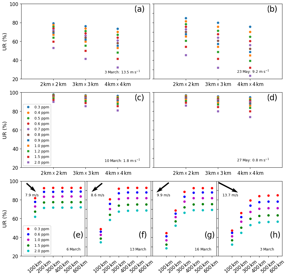
Figure 4 Uncertainty reductions (UR) from a 50 % prior uncertainty for the 6 h budgets of the Paris emissions. In panels (a)–(d), results are displayed for 4 different days characterized by different wind speeds, for different spatial resolutions of the satellite data (x axis) and for different precisions (colored markers). In panels (a)–(d), results are generated by considering a swath of 300 km. In panels (e)–(h), results are displayed for 4 different days characterized by different wind speeds, for different swaths of the satellite data (x axis), for different precisions (colored markers) and for a resolution of 2 km by 2 km.

The comparison between results obtained when doubling the random measurement error of the individual observations and when multiplying the value of their spatial resolution by 4 provides insights into the exploitation of the fine-scale patterns of the XCO₂ image by the inversion. Indeed, both changes result in doubling the resulting error at coarse resolution, but doubling the random measurement error at fine resolution conserves the capability to exploit information at this fine resolution, unlike coarsening the spatial resolution of the image. Figure 4a–d show that scores of UR with 2 km × 2 km resolution and 2 ppm precision data are extremely close to those with 4 km × 4 km resolution and 1 ppm precision data. URs with 2 km × 2 km resolution and 1.2, 1, 0.8 or 0.6 ppm precision data are also similar to URs with 4 km × 4 km resolution and 0.6, 0.5, 0.4 or 0.3 ppm precision data, respectively. This indicates that the inversions here do not really take advantage of the information on the fine-scale patterns of the plume from Paris.

A third set of inversions is conducted to study the sensitivity of the results to the width of the satellite swath while keeping all other observation and inversion parameters at reference values. This sensitivity is modulated by the wind conditions: the speed and direction of the wind control the spread and position of the plume and, thus, the value of the swath which fully covers the extent over which the amplitude of the plume is significant for the inversion, i.e., the value of the swath above which the results no longer change (Fig. 4e–h). This threshold value of the swath is lower for lower wind speed. For wind directions across the satellite track, the URs for the 6 h emissions of the Paris area are no longer sensitive to the increase in the swath above a value of 100 and 400 km for wind speeds lower than 8 and 9 m s⁻¹, respectively. The sensitivity to the swath is null (except if considering very low values for the swath of the order of the width of the plume from Paris) for wind directions along the satellite track as we consider satellite tracks centered on Paris.

3.2.3 Impact of the definition of the prior uncertainties in the CO₂ fluxes

The prior uncertainty covariance matrix B has a strong influence on the scores of posterior uncertainties when its “amplitude” is comparable to or much larger than that of the H^TRH matrix (see Eq. 2), i.e., once the prior uncertainties are comparable to or much larger than the projection of the observation errors in the control space. The relative prior uncertainty in the 6 h emission budgets (σ_Budget, Sect. 2.4), which characterizes the diagonal of B, is one of the critical drivers of the relative weight given by the inversion to the prior information and to the observations.

Thus, in a fourth set of inversions, we analyze the sensitivity of the inversion results for 6 h emission budgets to σ_Budget, with values for this parameter ranging between 0 % and 100 %. This set of inversions uses the reference values of the observation parameters and for the temporal autocorrelation of the prior uncertainties. Figure 5a–b show the corresponding results on 3 March (under strong wind) and on 10 March (under low wind) to highlight the dependence of this sensitivity to the wind speed. The curves of UR as a function of σ_Budget have an inflection point for values around 50 %. For low values of σ_Budget, the UR is sensitive to this parameter, the posterior uncertainty balancing the prior uncertainty and the projection of the observation error. For large values, the UR converges asymptotically towards 100 % and the posterior uncertainties are dominated by the projection of the observation error (i.e., the posterior estimate of the emission essentially relies on the top-down information from the observations). The observational constraint on the inversion is larger on 10 March than on 3 March as the wind is much lower on the former. As a consequence, the qualitative threshold for σ_Budget above which the URs are not very sensitive to this quantity is smaller on 10 March than on 3 March: 30 % and 50 %, respectively.

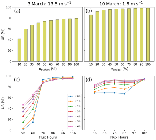
Figure 5 Uncertainty reductions (UR) as a function of the prior uncertainty (x axis) for 6 h budgets of the Paris emissions (a, b). Correlations between the prior errors on hourly emissions have a temporal length of 3 h (see Sect. 2.4). Panels (c) and (d) show the UR for the hourly emissions between 5 and 11 h (x axis) for several temporal lengths defining the correlations between prior errors on hourly emissions (colored dots), with “τ 0 h” referring to an absence of such correlations. Prior uncertainties on 6 h budgets of Paris emissions are taken to be equal to 50 % in panels (c) and (d). Columns represent 2 different inversion days: 3 March 2016 (strong wind) and 10 March 2016 (low wind). All inversion results are computed with a retrieval resolution of 2 km × 2 km, a precision of 0.6 ppm and a swath of 300 km.

These results over Paris suggest an empirical choice of a reference value for σ_Budget>50 %, in the absence of any factual knowledge about σ_Budget. With 50 % as a reference value, we focus our analysis of the posterior uncertainties on the projection of the information from the observations, and we almost neglect the prior information while retaining an assumption regarding the prior uncertainties that could seem consistent or even optimistic compared with series of assessment of the errors in inventories for cities at the daily scale (Wang et al., 2020). However, for other cities, for point or area sources with smaller amplitudes, the observational constraint is lower. The relative weight between the projection of the observations and the prior information is then more balanced than for Paris, and the prior uncertainty still has a significant impact on the posterior uncertainties when using σ_Budget=50 %. In order to study the pure projection of the observation errors, results using σ_Budget=100 % will be analyzed along with those using σ_Budget=50 % in Sect. 3.3.

The other important parameter defining the B matrix in this study is τ (Sect. 2.4). By construction, the increase in the corresponding autocorrelations in the prior uncertainties at the hourly scale in B does not modify the prior uncertainties in the 6 h emission budgets. However, it can help the inversion crossing the information on different hourly budgets to better constrain the overall budget of emissions. A fifth set of inversions with the reference values for the observation parameters and for σ_Budget is conducted to test the sensitivity to τ, with values for this parameter from 0 to 6 h (0 h indicating that there is no temporal correlation in B, and 3 h being the reference value), on 10 and 3 March. The analysis shows that the increase in τ hardly impacts the results for the 6 h budgets (not shown) but significantly changes the results for the hourly budgets (Fig. 5c–d). The autocorrelation brings information about the temporal distribution of the emissions, constraining how the 6 h emission budgets are distributed at the hourly scale. This impact is more significant when the XCO₂ signatures of the hourly emissions overlap, i.e., for hourly emissions between 05:00 and 07:00 LT when the wind speed is high and for almost all the hourly emissions when the wind speed is low. However, this better knowledge about the temporal variations from autocorrelations does not appear to improve the knowledge on the 6 h budgets.

3.3 Potential of satellite images for monitoring anthropogenic emissions at the regional, city and local scales

This section synthesizes the inversion results at the local (for power plants, industrial facilities) to regional scales over most of the model 2 km resolution subdomain, using a sixth set of inversions assimilating images that cover this subdomain entirely with a 900 km swath centered on Belgium (Fig. 1). This set of inversions covers all the days of March and May 2016 in order to analyze the impact of the wind speed and of the natural fluxes on the results. The prior relative uncertainties in the 6 h budgets of the emissions are alternatively set to σ_Budget=50 % and 100 %. These inversions use the reference parameters for the observation precision and resolution and for the temporal autocorrelation of the prior uncertainties in hourly emissions (0.6 ppm, 2 km × 2 km and 3 h, respectively). Results over most of the 2 km resolution subdomain using different observation spatial resolutions and precisions will briefly be discussed in Sect. 4.

3.3.1 Overview of the inversion performance

Figure 6 gives a geographical overview of the scores of UR in the 2 km resolution subdomain. The largest scores of UR for 6 h budgets are obtained for the megacities of Paris and London with mean values over the 2 months considered of >80 %. Mean UR can also be >60 % for several cities in Belgium and the Netherlands and for a large number of point sources (power plants and large industrial facilities) within the dense industrial area of western Germany, although these sources are close to each other or to other significant point and area sources.

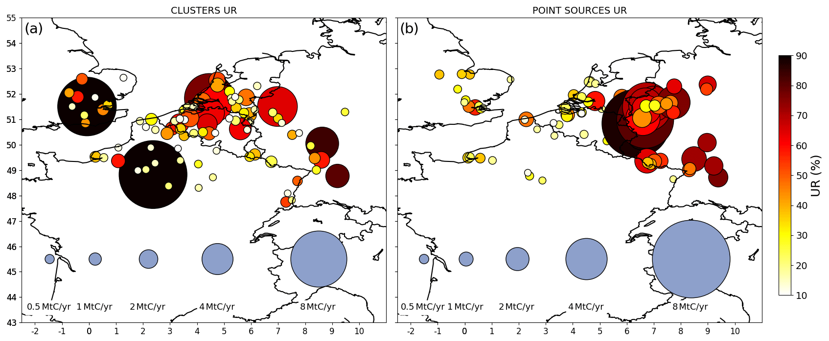
Figure 6 Mean uncertainty reductions (UR) for some city clusters (a) and some point sources (b) across the 62 inversion results for the days of March and May 2016. The areas and colors of the disks represent the annual emissions (MtC yr⁻¹) and the UR (%), respectively. The inversions are performed with a retrieval resolution of 2 km × 2 km, a precision of 0.6 ppm and a swath of 900 km. Prior uncertainties on 6 h budgets of clusters and point sources emissions are taken to be equal to 50 %, and prior error correlations have a temporal length of 3 h.

In a general way, the scores of UR increase with the magnitude of the emissions (Fig. 7). This increase is more important when considering lower emission values due to the asymptotic convergence of the UR towards 100 % for high emission values (with a point of inflection for sources of ∼ 2 MtC yr⁻¹ in the curves of Fig. 7). The increase in the UR as a function of the budgets of emissions is different if considering point or area sources. As expected, the largest URs are obtained for narrower sources like point sources (Fig. 7a) and cities (Fig. 7b) which generate plumes with smaller extents but larger amplitudes than diffuse countryside emissions. When using σ_Budget=100 %, the mean URs are larger than 50 % for all point sources and cities with an emission rate larger than 2 MtC yr⁻¹, while to achieve 50 % UR, an emission rate of at least 4 MtC yr⁻¹ is needed for regional countryside emissions (Fig. 7c). The gap is even larger when using σ_Budget=50 %, with mean URs that are systematically larger than 50 % for annual emission budgets of point sources and cities larger than 2 MtC yr⁻¹, but for annual emission budgets of regional countryside emissions larger than 7 MtC yr⁻¹.

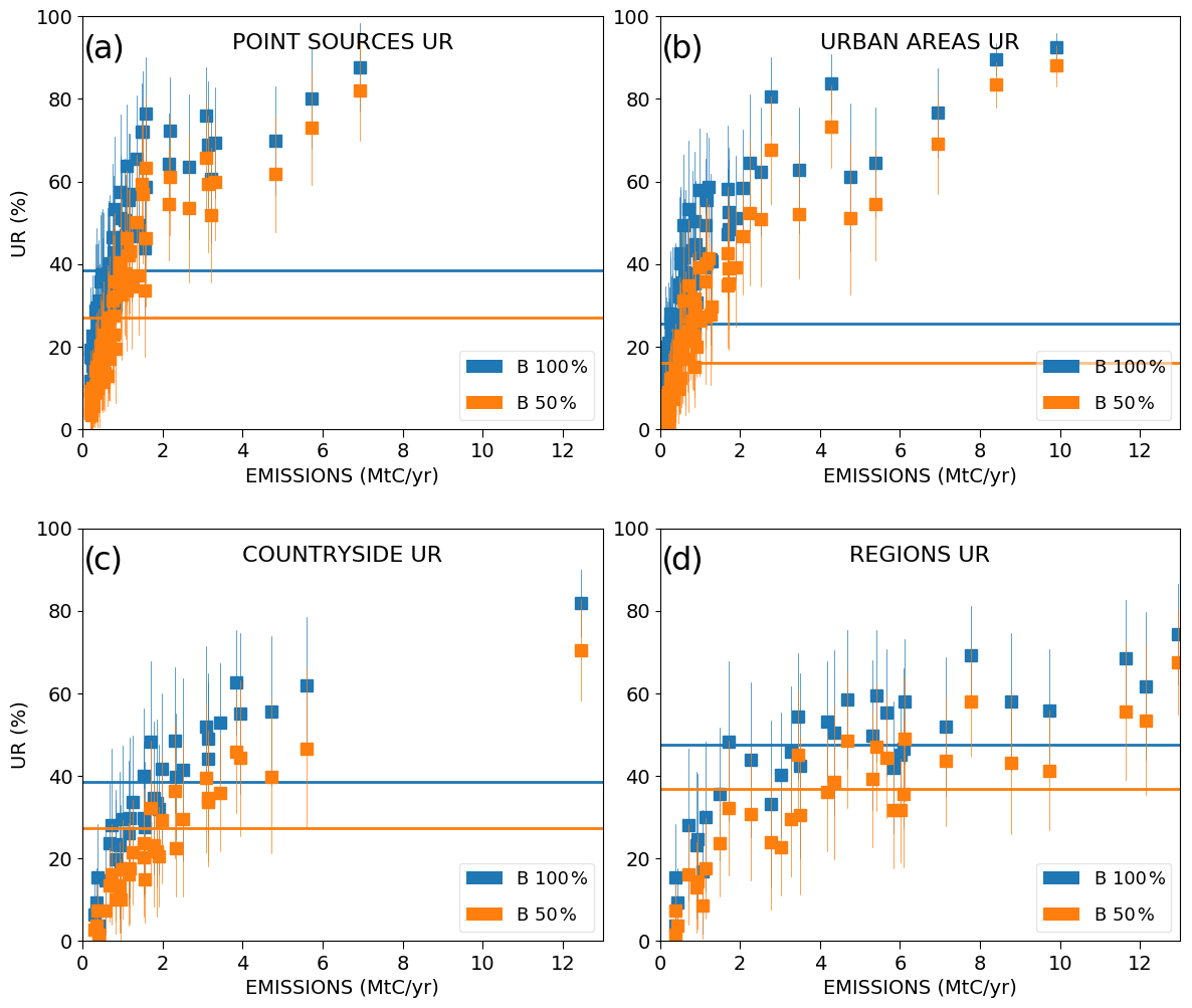
Figure 7 Mean values and standard deviations of the uncertainty reductions (UR) for the emissions of point sources (a), urban areas (b), countryside areas (c), and regions (d) across the 62 inversion results for the days of March and May 2016. The lines represent the averages of the temporal mean values across all sources of a given type. The emitting areas are chosen within the 2 km resolution domain of the model so that they are covered by the satellite track in order to avoid swath effects. Results are given as a function of the annual emissions (x axis) of the emitting areas. The inversions are performed with a retrieval resolution of 2 km × 2 km, a precision of 0.6 ppm and a swath of 900 km. Prior uncertainties on the 6 h budgets of the point sources, urban and countryside areas are taken to be equal to 50 % (orange squares) and to 100 % (blue squares). Prior uncertainties on the regional budgets are derived by aggregation of the prior uncertainties on their constituent emitting sources for both cases. Prior error correlations between hourly emissions have a temporal length of 3 h.

When aggregating the results for point sources, cities and countryside emissions at the regional scale, the relative prior uncertainty becomes significantly smaller than the values used for individual sources, as we assume that there is no correlation between their uncertainties: the mean prior uncertainty for the regions is then ∼ 33 % when assuming a 50 % prior error on the 6 h budgets of point sources, cities and countryside areas which make these regions. Moreover, the emission threshold above which the URs for the regional budgets are larger than 50 % becomes 10 and 7 MtC yr⁻¹ when using σ_Budget=50 % and 100 %, respectively (Fig. 7d). These thresholds are larger than those corresponding to individual point sources and cities as given above, but the overall performance of the inversion system at the regional scale is better with respect to that of the point sources and cities when analyzing the relative posterior uncertainties: for σ_Budget=50 %, the mean value is 22 % for the total regional budgets, whereas it is ∼ 40 % for the point sources' and cities' budgets (Fig. A1).

The results for the different types of sources are shown for four regions of Belgium in Fig. 8. This figure provides an illustration of the general results seen in Fig. 7. It shows that the URs for emissions of the largest urban areas (emitting more than 2 MtC yr⁻¹) are as high as those for the overall emissions of their respective region, although the budgets of emissions from these urban areas are much smaller than those of their regions. As suggested above, smaller prior uncertainties in the regional budgets lead to similar URs for cities' and regions' budgets, even though the relative posterior uncertainties in regional budgets are much smaller (Fig. 8b). When comparing point sources and cities that are characterized by the same prior uncertainty, the relative magnitudes of the URs are determined by the relative magnitudes of the emissions; thus, URs are much higher for the largest urban areas than for point sources and cities that emit much less CO₂. However, the comparison between the URs and emissions of the main cities and countryside areas of the regions of East and West Flanders illustrates that, even though they have lower emission budgets in these regions, cities are better constrained than countryside areas. This is in agreement with the enhanced capacity of the inversion system to monitor city emissions with respect to more diffuse emissions. This figure also qualitatively illustrates the ability of the inversion system to separate neighboring emission sources: the point source and city of Liège (left blue bar for the region of Liège in the figure) contained within the region of Liège are characterized by significant URs even though the point source is within the city of Liège and its plume is completely overlapped by the plume from the rest of the city. We will more systematically and quantitatively analyze the capacity of the inversion to disentangle the signals produced by neighboring sources in Sect. 3.3.3.

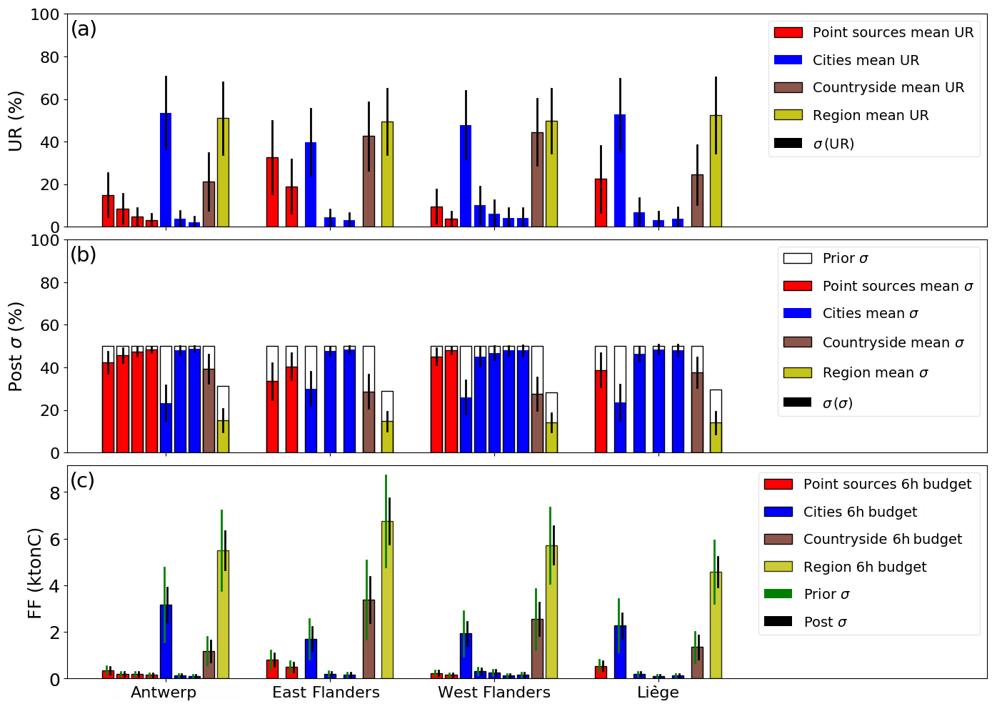
Figure 8 (a) Mean values and standard deviations of the uncertainty reductions (UR) for the regions, point sources, urban and countryside areas constituting four Belgian regions. Averaging is performed across the 62 inversion results for the days of March and May 2016. (b) Mean values and standard deviations of the relative post-uncertainty for each emitting area. Prior uncertainties are represented as well. Prior uncertainties in the regional budgets are derived by aggregation of the prior uncertainties of their constituent emitting sources (mean value ∼ 33 %). Panel (c) shows the mean 6 h budgets for each emitting area. The inversions are performed with a retrieval resolution of 2 km × 2 km, a precision of 0.6 ppm and a swath of 900 km. Prior uncertainties on the 6 h budgets of the point sources, urban and countryside areas are taken to be equal to 50 %, and prior error correlations between hourly emissions have a temporal length of 3 h.

The URs for the 6 h emission budgets show an important variability over the 62 inversion days as illustrated in Fig. 7. When using σ_Budget=50 %, the standard deviations of the day-to-day variations of the URs for the point sources, cities and countryside areas, are on average, equal to ∼ 12 %, ∼ 8.3 % and 12.2 %, respectively. These values are important with respect to the temporal mean of the values of UR (26 %, 16 % and 27 % when averaging across all the point sources, cities and countryside areas, respectively). These variations are associated with variations in the wind speed at the daily scale, as evidenced for the Paris case in Sect. 3.2.1. However, when considering results for the months of March and May together, they are also driven by the time profiles of the anthropogenic emissions that are characterized by a strong decrease in emissions between March and May due to the reduction of residential heating. Moreover, the UR variability is also determined by that of the uncertainties in the natural fluxes which are also very different from March to May. The natural fluxes have large negative amplitudes in May when they are dominated by the primary production and smaller positive amplitudes in March when they are mostly restricted to the heterotrophic respiration. Using constant prior relative uncertainties in the natural fluxes (as for the anthropogenic emissions) yields large absolute uncertainties in May and low absolute uncertainties in March. Furthermore, as the primary production related to photosynthetic processes is mostly driven by the radiative forcing and then by the daily variation in the cloud cover, natural fluxes and their prior uncertainties are also characterized by a strong day-to-day variability during the month of May; this is not the case in March due to a weak day-to-day variability in heterotrophic respiration. Cross sensitivity studies comparing the influence of the above drivers (not shown) indicate the predominant influence of the daily variability in the wind speed on the variability in UR for the anthropogenic emissions estimates for most sources. This conclusion should, however, be nuanced for some regions and countryside areas where the scores of UR for the anthropogenic emission estimates is highly impacted by the inversion of the natural fluxes and, thus, by the variability in these fluxes, during the month of May (see Sect. 3.3.2. below).

3.3.2 Impact of the uncertainties in the biogenic fluxes

The analysis of XCO₂ patterns produced by the different CO₂ fluxes (Sect. 3.1) suggests that the large signatures of the biogenic fluxes in May could impact the monitoring of the anthropogenic emissions. In order to weigh the impact of the uncertainties in biogenic fluxes, we conduct experiments where these uncertainties are ignored. In these experiments, the mean URs for the budgets of the regional and countryside anthropogenic emissions in May are equal to ∼ 31 % and ∼ 41 %, respectively (using σ_Budget=50 %). When accounting for uncertainties in biogenic fluxes, these mean URs decrease to ∼ 21 % and ∼ 31 %, respectively (Fig. 9c–d). This reveals that the inversion system had some difficulty separating countryside emissions from biogenic fluxes which is also illustrated by the important anticorrelations (−40 % on average) between the corresponding posterior uncertainties. During May, the smaller amplitudes and rather diffuse nature of countryside emissions with respect to natural fluxes (not shown) and the overlapping of their atmospheric signatures (Fig. 2) explain why the inversion system only has a limited ability to distinguish the countryside emissions. In contrast, during March, the smaller amplitude of natural fluxes compared with countryside emissions (not shown) explains why the inversion can better filter the signature of countryside emissions from that of natural fluxes.

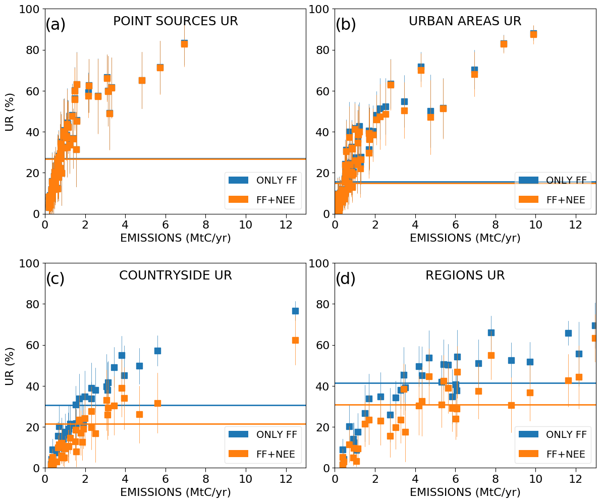
Figure 9 Same as Fig. 7 but the results are derived from inversions considering the anthropogenic emissions only (blue markers) and from inversions considering the natural fluxes as well (orange markers). Prior uncertainties on the 6 h budgets of the point sources, urban and countryside areas are taken to be equal to 50 %, and prior error correlations between hourly emissions have a temporal length of 3 h. Prior uncertainties on the regional budgets are then derived by aggregation of the prior uncertainties of their constituent emitting sources (mean value ∼ 33 %).

Contrary to the URs for countryside emissions and regional budgets, the URs for the point sources and cities are hardly impacted by the uncertainties in biogenic fluxes during the month of May, even when the emission budgets of these sources are smaller than 1 MtC yr⁻¹ (Fig. 9a, b), and even though these budgets are quantitatively lower than the absolute value of the regional budgets of biogenic fluxes. Consistently, the posterior uncertainty in the inverted 6 h budgets of the emissions of cities or point sources is weakly correlated with that in the 6 h budgets of biogenic fluxes in their respective region (−2 % and −5 % on average for the cities and point sources, respectively). Therefore, the visual inspection of Fig. 2 may wrongly suggest that the plumes of the smallest point sources and cities controlled individually can hardly be separated from the signature of biogenic fluxes. The differences in terms of spatial scales of the atmospheric signatures appear to be the main driver of the skill of the inversion to separate anthropogenic sources from biogenic fluxes.

3.3.3 Separation of the different anthropogenic emission sources

In order to estimate the ability of the inversion system to monitor anthropogenic sources whose atmospheric signals overlap separately, we focus on pairs of sources contained within the same region and assess whether the sum of the variances (Var) associated with the inverted emissions for each source is comparable with the absolute value of their covariance (Cov), which is nearly systematically negative as a result of the uncertainty in the spatial attribution of emitted CO₂ to individual sources in the inversion. This criterion means, if the covariance is negative, that the variance associated with the ensemble of the two sources is much smaller than the sum of the variances associated with each source. Indeed, the variance of the sum of two random variables X_a and X_b is given by $\mathrm{Var}\left(X_a+X_b\right)=\mathrm{Var}\left(X_a\right)+\mathrm{Var}\left(X_b\right)+\mathrm{2}\cdot \mathrm{Cov}\left(X_a+X_b\right)$. In terms of inversion, this case describes a situation where a pair of sources is much better constrained than each of its individual sources ($\mathrm{Var}\left(X_a+X_b\right)\ll \mathrm{Var}\left(X_a\right)+\mathrm{Var}\left(X_b\right))$, i.e when the inversion system does not entirely manage to disentangle overlapping signals and to independently constrain each source.

Figure 10 indicates that the system generally has a good ability to independently constrain the different sources within a given region: point sources, cities, countryside areas and natural fluxes. In this figure, the number of pairs of sources that are characterized by an important negative covariance term ($\mathrm{2}\cdot \mathrm{Cov}\left(X_a+X_b\right))$ compared with the sum of the individual variances (Var(X_a)+Var(X_b)) is indeed much lower than the number of pairs of sources that are characterized by a relatively small covariance term. Only 20 pairs of sources out of a total of 890 pairs show a covariance term that is larger than 25 % of the sum of the variances (squares below the blue line in Fig. 10a). Most pairs for which the inversion system may be unable to distinguish individual sources in a completely independent way consist of a point source and its surrounding urban or countryside area. Only one case consists of two point sources that are located close to each other near Karlsruhe in Germany, and no cases consist of pairs of urban–urban or urban–countryside areas. The 20 cases of less separable pairs of sources identified above could be associated with situations for which the inversion system could have difficulties independently monitoring two sources, but this conclusion should be nuanced when all terms (sum of the variances and covariances) are small: for example, four pairs of sources characterized by important negative correlations show an UR for each individual sources which is larger than 50 % (squares in the top-right quadrant of the Fig. 10b). For these cases, the problem of distinguishing between the two sources applies to a moderate residual posterior uncertainty, and the inversion still gets a relatively precise estimate of the emissions.

Figure 10 (a) Post-variances of the emission estimates for pairs of anthropogenic sources contained within a same region function of the covariances between the individual sources of the pairs. The colors of the markers correspond to the UR of the pairs. (b) Comparison of the URs for individual sources within each pair of anthropogenic sources contained within the same region: each symbol corresponds to a pair, with the UR for one of the two sources being given by the y axis and the UR for the other source being given by the x axis. The colors of the markers correspond to the UR of the pairs. The regions corresponding to this plot are contained within the 2 km resolution area of the model. Results are derived with an instrumental resolution of 2 km × 2 km, a precision of 0.6 ppm and a swath of 900 km. Prior uncertainties on the 6 h budgets of the point sources, urban and countryside areas are taken to be equal to 50 %, and prior error correlations between hourly emissions have a temporal length of 3 h. Pairs of anthropogenic sources are made up of point sources and of urban and countryside areas.

Moreover, a low covariance between sources can often be explained by the lack of constraint on their total budget or on one of the two sources, rather than by a good separation between the two sources. Examples of pairs of sources with an important UR for their total emissions and a small covariance while only one individual source in each pair is well constrained can be seen in the top-left and bottom-right quadrants of Fig. 10b (where the UR for the total is larger than 75 %, while one of the sources shows an UR lower than 20 %). Pairs of sources characterized by relatively low values of covariance but small values of UR for both the total and the two sources are identified in the top-right quadrant of Fig. 10a and the bottom-left quadrant of Fig. 10b. These pairs are characterized by low individual sources and total emissions whose amplitudes are below the thresholds required by the inversion system to produce reliable estimates (see Sect. 3.3.1).

4 Discussion

Our series of tests and analysis demonstrate the potential of our inversion system for exploring various aspects of the estimation of anthropogenic CO₂ emissions based on satellite XCO₂ spectro-imagery.

4.1 A performance simulation tool

The analytical formulation of the inversion makes it easy to test different scenarios of observation systems that monitor anthropogenic emissions; however, in this study, the OSSEs with the inversion framework have been performed in order to investigate the potential of the satellite imagery of XCO₂ from helio-synchronous orbits only, depending on instrumental configurations or other factors such as the wind or the amplitude of the emissions. Such spaceborne imagery similar to CO2M may become the critical component of operational atmospheric inversion systems for the monitoring of CO₂ anthropogenic emissions. These operational inversion systems will likely have to jointly assimilate data from many of the existing satellite missions, from ground-based networks and from the planned spectro-imagers. Moreover, in addition to CO₂ concentrations, co-emitted pollutants and radiocarbon should be assimilated as well. Ultimately, OSSEs would have to integrate all of these components of the observation system (Ciais et al., 2015; Pinty et al., 2017). However, we need OSSEs considering the spaceborne imagery of XCO₂ as a stand-alone system to determine the instrumental parameters ensuring that this imagery can bring emission estimates with sufficient coverage and accuracy so that it can serve as a backbone for the operational monitoring of emissions. Furthermore, in a context where there is a lack of ground-based and spaceborne networks that are suitable for the monitoring of CO₂ anthropogenic emissions, these OSSEs can help better understand the needs in terms of complementary observation components.

The analytical inversion system built for this study allows for an important set of observational parameters and situations to be tested. Once the atmospheric transport functions associated with the different sources have been computed, the derivation of the posterior uncertainties is fast and results can be delivered for a wide and detailed range of specifications on the spatial resolution, precision (focusing here on the errors in XCO₂ from the instrumental noise) and swath of the satellite XCO₂ images. Extending the study of Broquet et al. (2018), the sensitivities of the inversion results to these three parameters have been tested on the example of the inversion of the emissions of Paris (Sect. 3.2.2.). We varied these parameters without accounting for current limitations in space technologies (or for cost issues) which impose potential trade-offs between their configurations. The impact of the wind speed on the determination of the 6 h and hourly budgets of the emissions is analyzed by assimilating images over different days of March and May. Finally, the flexibility of the inversion system also allowed for the impact of the way that prior uncertainties in the fluxes are prescribed to be tested.

The inversion framework produces curves of sensitivity that give several qualitative and quantitative insights into the optimal configurations of the satellite imagery: the study of the UR for the Paris emissions indicates (i) that a 4 km × 4 km spatial resolution is sufficient, provided that the precision at this spatial resolution is very high, and (ii) that the inversion hardly makes use of patterns at a finer spatial resolution. However, as discussed in Sect. 3.2, this might come from the relatively large extent of the plume from Paris as well as from the distances between this plume and other major plumes. Thus, we have extended the analysis of the sensitivity to the observation spatial resolution and precision to all of the days of March and May and to the ensemble of controlled regional, city and local sources (as for the analysis in Sect. 3.3) testing a reduced set of resolutions and precisions. The results are displayed in Fig. 11. This experiment confirms that results for point sources and narrow cities are more sensitive to the availability of the information at the reference resolution of 2 km than that for Paris. The UR for point sources and cities emitting less than 2 MtC yr⁻¹ is larger with a spatial resolution of 2 km × 2 km and a precision of 1.2 ppm than with a spatial resolution of 4 km × 4 km and a precision of 0.6 ppm, (i.e., with the same precision at a 4 km resolution but without information about the patterns at scales finer than 4 km). However, the differences are not really significant, and Fig. 11 tends to confirm that a spatial resolution of 4 km × 4 km would be fine if achieving a very good precision: typically, 0.3 ppm if one is willing to get the results from the reference configuration of the observation with 2 km resolution and 0.6 ppm precision. With a 2 km × 2 km resolution, the mean URs for all types of emissions would increase on average by 10.1 ± 1.5 % if the precision increased by a twofold factor (from σ=1.2 to 0.6 ppm and from 0.6 to 0.3 ppm). While this represents a dramatic increase in the UR when changing the precision from 1.2 to 0.6 ppm, the relative impact is smaller from 0.6 to 0.3 ppm, and the reference value of 0.6 ppm precision at a 2 km resolution appears to be a balanced option. Finally, the results for the Paris case point out that, at the reference precision of 0.6 ppm, the performance of the inversion system would be nearly equivalent at 2 km × 2 km and 2 km × 3 km resolutions (Fig. 4). Thus, the spatial resolution could be relaxed to 2 km × 3 km compared with the reference resolution without degrading the precision of the inversions very much.

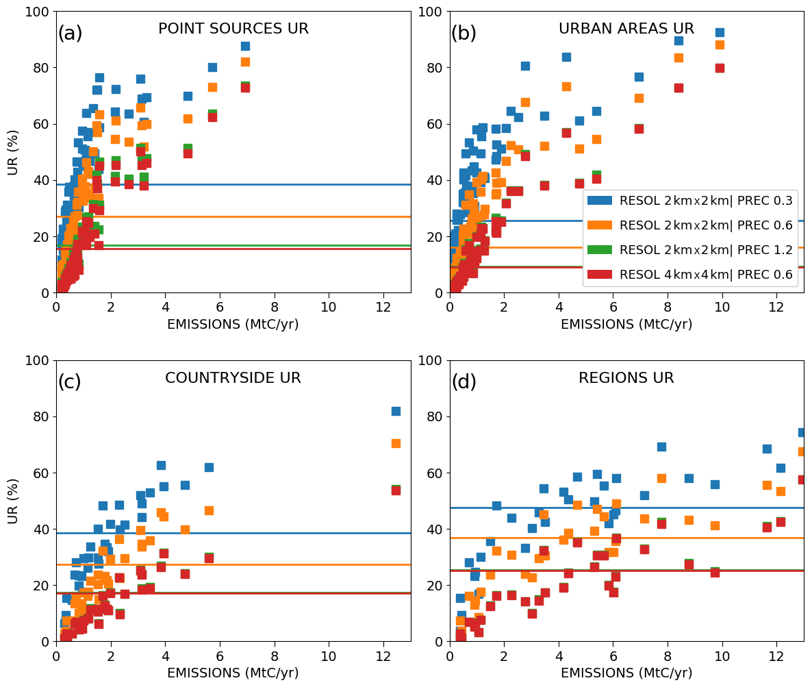
Figure 11 Same as Fig. 7 but the inversions are performed with different retrieval resolutions and precisions (swath = 900 km). Prior uncertainties in the 6 h budgets of the point sources, urban and countryside areas are taken to be equal to 50 %.

If we consider the monitoring of the Paris emissions, the impact of the swath on the results is limited for swaths larger than 400 km (Sect. 3.2.2; Fig. 4). As the megacity of Paris produces plumes whose intensity and extent are amongst the highest with respect to anthropogenic emissions sources in western Europe, this supports the use of a swath close to 400 km to ensure that the full extent of plumes from targeted sources near the center of the satellite field of view is caught. However, a narrower swath would be sufficient for the large majority of cities which emit less than Paris and, thus, have shorter plumes. This would impact the monitoring of the large megacities emitting more than 10 MtC yr⁻¹ like Paris, which represent around 9 % of the emissions from cities and power plants over the globe (Wang et al., 2020), but this impact is limited for Paris in most meteorological conditions as long as the swath is larger than 250 km (90 % of the cases for the 62 d of inversion, not shown). A general conclusion from these results is that the swath is a less critical parameter than the pixel precision and resolution.

Overall, these results support the reference configurations for the pixel resolution and precision and for the swath width that broadly correspond to the current ones for the CO2M mission, even though they suggest a relaxation of the spatial resolution to 2 km × 3 km and an extension of the swath up to 400 km. However, as this study does not account for technical and cost trade-offs between these parameters, it cannot provide a full assessment for their combination. Furthermore, by flying a satellite over the areas of interest on any day in the sensitivity tests, we restrained the role of the swath to covering a more or less important portion of the plumes, with a lack of sensitivity when the swath exceeds the plume length or when the wind blows along the satellite track. In practice, a critical role of larger swaths (like that of using more satellites in a constellation) is to increase the number of situations for which the plume from a given city can be seen, which is ignored in this study. Finally, the spatial resolution could also play a role when accounting for cloud cover as it could help to increase the spatial coverage. A more realistic simulation of the observation sampling by specific missions or constellations, with one or several satellites following real tracks and including the impact of cloud coverage and large aerosol loads, and some realistic technical constraints between the parameters, is needed to fully assess the right balance between higher precision, finer spatial resolution and larger swaths.

4.2 Ability to monitor anthropogenic emissions at the regional, city and local scales

At first, a qualitative overview of the atmospheric signatures could imply that the ability of the inversion system to quantify the budgets of emissions from most of the 84 large point sources and from the two megacities of Paris and London should be much larger than for smaller cities and that countryside emissions should hardly be constrained by the inversion (Sect. 3.1). However, the quantitative analysis of the results from the OSSEs described in Sect. 3.3. shows that the detection capacity of the inversion system is equivalent for point sources and cities: uncertainties in both types of sources emitting more than 2 MtC yr⁻¹ are reduced on average by more than 50 % when the resolution and precision of the satellite data are equal to 2 km × 2 km and to 0.6 ppm, respectively, and when the prior uncertainties in the fluxes have been set to 50 % of the 6 h budgets (Sect. 3.3.1). With the same parameters, the threshold on the level of emissions to get such an UR is much higher (∼ 10 MtC yr⁻¹) for the countryside areas and for the whole regions. However, for these types of sources, the overall level of performance of the inversion system is still comparable to that for point sources and cities: for the 67 regions considered in this study, the mean URs for the total emissions and for the countryside emissions are 37 % and 27.4 %, respectively (Sect. 3.3.1). The lower performance of the inversion system to monitor the countryside and regional anthropogenic emissions could be partly related to the impact of the biogenic fluxes on the determination of these types of emission sources contrary to the point sources and cities (Sect. 3.3.2). Beside these sensitivities to the source amplitudes and to the uncertainties in biogenic fluxes, the variations in URs are also driven by the wind (Sect. 3.2.1 and 3.3.1) and by the potential loss of part of the atmospheric signatures of sources at the edges of the satellite swath (Sect. 3.2.2).

We have also investigated the capacity of the inversion system to deal with the overlapping of XCO₂ plumes produced by nearby sources (Sect. 3.3.3). As satellite images give snapshots of the XCO₂ distribution at a given time (11:00 LT) and as atmospheric transport mixes the contribution of the different sources over the 6 h before the satellite overpass, it is important to assess the ability of the inversion system to disentangle the information coming from different sources at different times. With the hypothesis adopted in this study, most point sources and cities can be monitored independently by the inversion system. This ability could be partly related to the high-resolution modeling that allows for the description and capture of the fine-scale patterns of the XCO₂ signatures of the point sources even if the inversion is weakly sensitive to patterns at scales <4 km (Fig. 11).

Beyond the capacity to monitor the emissions of point sources, urban and countryside areas separately, the additional benefit of separately controlling these emissions within a given region is the mitigation of the aggregation errors when inverting the total budget of a region. In analytical inversions, these errors arise when a control of the emissions at an overly coarse resolution excessively limits the ability to fit the actual spatial distribution of the emissions and of the concentrations. These errors are evidenced for our study by inverting regional budgets without considering any internal separation into cities, point sources or countryside areas in the control vector: with such a configuration, the results are significantly and incorrectly more optimistic than those obtained with the inversions that use this subdivision (Fig. A2).

4.3 An optimistic framework

This study aims at assessing the projection of the sampling and observation random noise into the emission estimates. It combines optimistic assumptions that prevent the supposition that the level of posterior uncertainties achieved in the OSSEs here should correspond to that of the inversions with real data. The ability of the inversion system to separately monitor point sources and cities (Sect. 3.3.3) and to quantify regional budgets of diffuse emissions is partly due to the underlying assumption made in this study that the atmospheric transport is perfectly known. We ignored the transport modeling errors and implicitly supposed that the position and extent of the XCO₂ plumes from cities or point sources are perfectly simulated. Accounting for the transport modeling errors by assuming that they can be described as a random noise uncorrelated in space and time, as is usually done in atmospheric inversions, would not fundamentally change the results of this study. The impact of such an error would be equivalent to decreasing the precision of the observations. However, as a consequence of errors in the wind speed and direction, or in the CO₂ transport model itself, the simulation of narrow and localized plumes can poorly match the actual plumes and can strongly affect the inversion of the emissions from point sources and cities. The simulation of the signature of diffuse emissions could also be different in terms of shape and extent from the actual signature of these emissions. An inversion procedure that would simultaneously control both transport parameters and CO₂ emissions within a coupled meteorological–CO₂ transport model (Kang et al., 2011) may partially address these issues, although it would greatly increase the complexity of the inversion, in particular by introducing potentially large nonlinearities in the observation operator. New methods based on imagery processing (Corpetti et al., 2009), plume detection (Kuhlmann et al., 2019), Gaussian plume modeling (Nassar et al., 2017) or direct computation of fluxes through detected plumes may also help overcome realistic transport uncertainties to invert the emissions corresponding to point sources and cities (Varon et al., 2018). However, these methods may hardly deal with diffuse emissions whose signatures have low amplitudes and should be difficult to detect in XCO₂ images. Thus, the recovery of countryside emissions and of regional budgets of the emissions may be optimistic in this study.

Moreover, the configuration of our inversion system uses many of the traditional assumptions of atmospheric inversions, including the rather simple characterization of the sources of uncertainties with Gaussian distributions, which may underestimate their impact. The perfect knowledge of the statistics of the different source of uncertainties that are accounted for is another traditional optimistic assumption used in atmospheric inversions with synthetic data and in the experiments here. Furthermore, some sources of observation errors, such as the systematic errors that bear spatial correlations, are purposely ignored in the present study. Such errors exacerbate the problem of the identification of the signatures of point source, city to diffuse emissions, in addition to having a larger error budget than random noise at the spatial scales of such signatures. There is a clear need to assess the impact of such correlated errors. Lastly, the extent of the observation sampling is made rather optimistic by ignoring cloud cover and the loss of data due to large aerosol loads. Generally, the results of this study could be seen as optimistic and as an upper limit of the skill of the inversions using satellite images only, but they could also be viewed as a good indicator of the sensitivity of the uncertainty reduction to various parameters and drivers.

Broquet et al. (2018) provided insights into the impact of cloud cover and systematic errors in the XCO₂ images. They used realistic simulations of satellite samplings and errors made for the CarbonSat mission by Buchwitz et al. (2013a). Results have indicated that, when accounting for cloud cover, the satellite data could efficiently constrain emissions from Paris only ∼ 20 d per year and that the impact of the systematic errors anticipated for the mission is such that the system would hardly be able to reduce errors in the emission estimates if these errors were not filtered or controlled for. However, efforts have been made to limit the amplitude of systematic errors in the concept of the new CO2M mission.

Our new inversion framework allows for a realistic simulation of the observation sampling and errors to be accounted for. Nevertheless, generating simulations of the systematic errors from the retrieval of XCO₂ data that are suitable for the purpose of our study would have been difficult. Systematic errors are not described in the uncertainties computed by existing retrieval schemes. Furthermore, they depend on specific measurement configurations and on the evolving skill of radiative transfer inverse models and of empirical bias-correction systems, so that their characterization based on diagnostics with existing missions may hardly apply to future missions. Simulating realistic patterns of cloud cover consistent with the meteorology for the different test cases investigated would have also been challenging. Finally, this study focuses on other parameters to allow for an in depth exploration of the sensitivity of the inversions to these parameters.

In order to gain insight into the impact of errors with spatial patterns such as model and systematic errors, we have conducted experiments where spatial correlations are included in the observation error (in the R matrix). We have tested isotropic and homogeneous spatial correlations exponentially decaying with distance, using various correlation lengths. The experiments and results are described in Appendix A, as they are outside the scope of this study. The results indicate that including correlations in the observation errors tends to increase the budget of observation errors and, thus, to increase the posterior uncertainties in the flux estimates as long as the correlation length scale does not exceed that of the signature of the fluxes in the XCO₂ images. However, including correlations in the observation errors also tends to increase the ability to distinguish between the patterns of the observation error and of the signatures of the fluxes and, thus, decreases the posterior uncertainties; therefore, for large spatial correlation lengths, increasing the correlation length leads to a decrease in the posterior uncertainties. In our tests, the worst situation for the monitoring of the emissions in the study area corresponds to ∼ 10 km correlation length scales. These results should be interpreted cautiously, as the spatial patterns of the model and systematic errors are more complex than this traditional but simple modeling of spatial correlations. Furthermore, in our tests, the inversion system is perfectly informed about the statistics of the observation error which would hardly apply in practice. Future studies will integrate more realistic simulations of observation sampling and errors from different concepts of spaceborne imagery, based on radiative transfer inverse modeling applied to realistic fields of surface and atmospheric conditions and instrumental specifications.

A last significant simplification of the general problem of the inversion of the anthropogenic emissions based on XCO₂ data has been stressed by Ciais et al. (2020). Anthropogenic emissions of CO₂ bear a major share of emissions from biofuel combustion which can hardly be separated spatially from the fossil fuel combustion component. Furthermore, the emissions of CO₂ by human respiration represent a significant portion of the total CO₂ emitted from cities. The XCO₂ data and the atmospheric inversion approaches can hardly be used to distinguish between these different components if they cannot rely on complementary data. This factor was ignored here, as well as in most of the studies dedicated to the inversion of anthropogenic CO₂ emissions at city to regional scales.

4.4 Exploiting further capabilities of the inversion framework: potential of complementary observation systems and results at larger temporal scales

Our analysis is restricted to a window from 05:00 to 11:00 LT corresponding to the period which might be constrained by the satellite observation from a heliosynchronous satellite with a 11:00 LT overpass. This provides little information about the capacity of the inversion system to monitor daily to monthly budgets. To address this need and improve the results of the inversions, the modularity of our data assimilation framework could integrate multiple streams of data in order to increase the temporal and spatial coverage of the information (Moore et al., 2018; O'Brien et al., 2016).

In future studies, our inversion system could also integrate more realistic hypotheses concerning the description of the prior uncertainties in the emissions. Uncertainties in inventories are indeed difficult to characterize, and this study assumed, rather arbitrarily, that the relative uncertainty in the 6 h budgets was of 50 % or 100 % (Sect. 2.4). We also assumed that the prior uncertainties had low temporal correlations, i.e., correlation over timescales of less than 6 h, and we neglected the spatial correlations between the budgets for the different point sources, cities and countryside areas. Actual anthropogenic emissions and inventories have complex cycles at daily and weekly scales as well as a large temporal and spatial variability. There is still a critical lack of knowledge and of characterization of the correlations in the uncertainties in the inventories (Wang et al., 2018, 2020). However, some extensive analyses are now conducted to fill this gap (Super et al., 2020). We can expect some stronger spatial and temporal connections than assumed in this study, which would increase the transfer of information from the atmospheric observations, i.e., both the uncertainty reduction for the sources and time windows covered by the observations, and the uncertainty reduction for other sources, time windows, and for large spatial and temporal scales.

5 Conclusions

We have presented a new and comprehensive high-resolution atmospheric inversion system to assess the potential of the satellite imagery of XCO₂ for the monitoring of anthropogenic emissions from local to national scales. This system has been designed to deal with a wide range of different sources in terms of emission amplitude, distribution and spatial scale and to account for the overlapping between the signatures from different anthropogenic sources and natural sources and sinks. To cover the local and regional scales while mitigating computational costs, this inversion system is based on an atmospheric transport model with a zoomed grid whose horizontal resolution ranges from 2 km in the most resolved domain to 50 km at its edges. The area of highest horizontal resolution (2 km) encompasses regions where the hourly emission budgets of a large ensemble of cities and point sources are inverted separately, i.e., that of northern France, Belgium, the Netherlands, western Germany, Luxembourg and London. Urban areas are delimited using a clustering algorithm, and large industrial plants are selected based on an emission threshold. In total, the system controls the hourly budgets of 303 different anthropogenic sources (plants, cities or regions), the hourly budgets of biogenic fluxes for 67 regions and a scaling factor applied to the initial, lateral and top boundary conditions for each inversion window.

The study investigates the potential of imagery of XCO₂ from satellites on helio-synchronous orbits that are similar to CO2M but vary with respect to the spatial distribution, precision and swath of the imagery. The aim is to analyze the relative sensitivities to these different parameters and, thus, to gain insight into the optimal configurations of new satellite imagery concepts. In the synthetic framework of our experiments, we simulate satellite overpasses over the area of interest at 11:00 LT, and we conduct inversions with windows covering the 6 h before these overpasses (05:00–11:00 LT), which have been identified as the periods that might be directly constrained by the satellite observations. Focusing on the instrumental noise, the analysis of the sensitivity to the errors on XCO₂ data ignores systematic errors from the retrieval process. Moreover, all images are assumed to be taken under clear-sky conditions with the swath centered on the targeted sources. Another critical point is that the transport modeling errors are ignored. Finally, (i) the optimal spatial coverage of the targeted plumes which are seen entirely except during the tests of sensitivity to the swath width, (ii) the lack of systematic and transport modeling errors, and (iii) the assumption that the inversion system is perfectly informed about the statistics of the errors in the prior estimates of the emissions, biogenic fluxes and transport model boundary conditions, raise optimistic scores of URs. However, these scores are mainly analyzed in terms of the upper bound of what can be achieved by the assimilation of the satellite images or in a relative way when diagnosing sensitivities to various parameters. The results of the sensitivity studies support specifications for the pixel resolution and precision as well as the swath width that are close to those considered for CO2M: combinations of a 2 km × 2 to 2 km × 3 km pixel spatial resolution, 0.6 ppm precision and 250 to 400 km swath. More constraining options do not appear to cause significant enough improvements in the precision of the emission estimates. The inversions illustrate a higher skill with respect to monitoring individual point sources and dense cities. However, despite their optimistic configuration, they also indicate that scores of URs of more than 50 % for the 6 h emissions before the satellite overpasses can be achieved for cities and point sources emitting more than 2 MtC yr⁻¹ only (with a configuration where the resolution and precision of the satellite data are equal to 2 km × 2 km and to 0.6 ppm, respectively, and where the prior uncertainties in the 6 h emissions have been set to 50 %).

Exploiting the modularity of our inversion system and coupling it to radiative transfer inverse models, future studies should be conducted to assess the performance of more specific concepts of spaceborne imagery under more realistic scenarios regarding sampling, XCO₂ retrieval errors and cloud cover. They should also analyze the complementarity of the imagery from helio-synchronous orbits with ground-based measurements or with different types of spaceborne observation sensors.

Appendix A: Testing the impact of spatial correlations in the observation error

When addressing the impact of errors from the atmospheric modeling and observation, our study focuses on the random error from the satellite instrumental noise which is assumed not to bear spatial correlations (following, e.g., Buchwitz et al., 2013a). It does not consider the impact of two major sources of uncertainties in the inversions: the transport modeling errors and the systematic errors in the XCO₂ retrievals from the inverse radiative transfer modeling (Hobbs et al., 2017). These errors raise spatial correlations in the overall observation errors (Worden et al., 2017; Broquet et al., 2018).

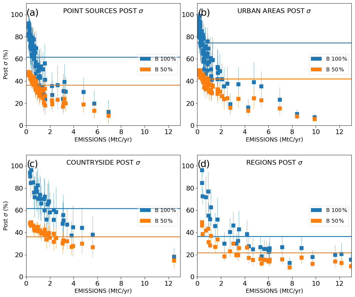
Figure A1 Same as Fig. 7 but the relative posterior uncertainties are shown instead of the UR.

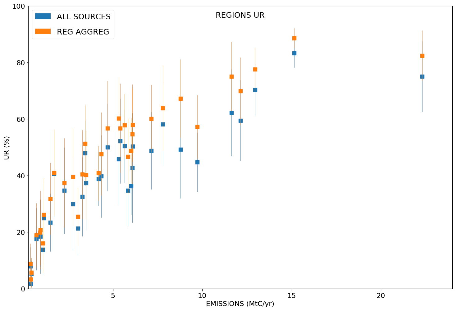
Figure A2 Mean values of the uncertainty reductions (UR) of the emissions at the regional scale across the 62 inversion results for the days of March and May 2016. Results are given as a function of the annual emissions (x axis). Regional emissions are inverted with (blue markers) and without (orange markers) considering an internal separation of the region into cities, point sources or countryside areas.

Besides the need to limit the scope of the study to a reasonable extent, one reason for not studying the impact of these errors here is that they depend on the specific modeling and measurement configurations as well as on the evolving skill of transport and radiative transfer models and of empirical bias-correction systems (see, e.g., the dramatic improvement of the agreement between NASA's Orbiting Carbon Observatory-2 retrievals and reference ground-based retrievals between version 7 and version 8 of NASA's algorithm in Fig. 18 of O'Dell et al., 2018). Therefore, conclusions from existing missions may hardly apply to future ones. Another reason for not considering these errors is that they are characterized empirically, and we still lack robust and theoretical ways to describe them. However, in order to feed the discussion and perspectives regarding such errors, we provide a first exploration of the impact of spatial correlations in the observation errors.

A traditional way to model spatial correlations between observation errors is to assume that they decrease with distance and that they are isotropic and homogeneous in terms of spatial scale (Chevallier, 2007). Therefore, we model such correlations using exponentially decaying functions $\left(\exp \right(-d/D\left)\right)$ of the distances d between two observation pixels, with the parameter D defining the correlation length scale. Their inclusion in R (Sect. 2.3.1) is tested by applying such correlations to the total observation errors, i.e., not defining the total observation errors as a combination of spatially correlated and uncorrelated errors but as a single component with spatial correlations. This choice eases the analysis of the impact of spatial correlations here, which aims to gain first general insights into the behavior of the inversion when including them rather than to provide quantification of such an impact.

In a new set of tests with our inverse modeling framework, we use the setup which covers the sources over most of the 2 km resolution model subdomain based on 900 km wide XCO₂ images (Sect. 3.3). We set R with a 1σ uncertainty of 0.3 ppm for all XCO₂ data and with D=10, 50 or 100 km. In order to lighten the computational load associated with the inversion of a matrix R that is no longer diagonal (Eq. 2), we perform the inversions by considering observations with 4 km resolution pixels rather than 2 km resolution pixels. Thus, the choice of a data precision of 0.3 ppm allows one to obtain results for a configuration that is close to the reference configuration (with a data resolution and precision of 2×2 km² and 0.6 ppm, respectively; see Sects. 3.2.2 and 4 regarding the similarity of the results from the inversions carried out with a given instrumental precision and resolution and the inversions carried out with an instrumental precision 2 times smaller and a resolution 4 times larger).

When introducing correlations with small spatial scales (D=10 km), the uncertainty reductions for all type of emission sources are lower than for the inversions performed without correlations within the R matrix (Fig. A3). When using D=50 km, this is still true for most of the cities and for countryside and regional emission areas. However, the uncertainty reductions become larger than when ignoring spatial correlations for all point sources (except two point sources) and the cities that emit less than ∼ 25 MtC yr⁻¹. Finally, when using D=100 km, the uncertainty reductions become larger than when ignoring spatial correlations for all point sources, all cities emitting less than 40 MtC yr⁻¹, and a significant number of countryside and regional emission areas. This behavior, the analysis of images of the plume from Paris with the different types of observation errors tested here (Fig. A4), the fact the cities with the largest emission rate are generally also those with the largest spatial extent, and the fact the sources with larger emission rates have an atmospheric signature which can be distinguished on larger spatial extent, lead us to the following interpretation of the impact of the spatial correlations in R:

• when introducing correlations with small spatial scales in R, the posterior uncertainties in flux estimates increase as these correlations yield larger budget of observation errors at the scale of the signatures of the targeted fluxes. This impact tends to saturate when the spatial correlation scale in R reaches and becomes larger than the scale of the signatures of the targeted fluxes.

• Conversely, the increase in the correlation scales helps the inversion separate the observation error patterns from these signatures.

• These two opposing effects lead to a worst-case scenario in terms of posterior uncertainties in the emission estimates that correspond to correlation scales in R that are function of the scale of the flux atmospheric signatures. In particular, this varies depending on whether we analyze results for point sources, cities or widespread emissions across regions.

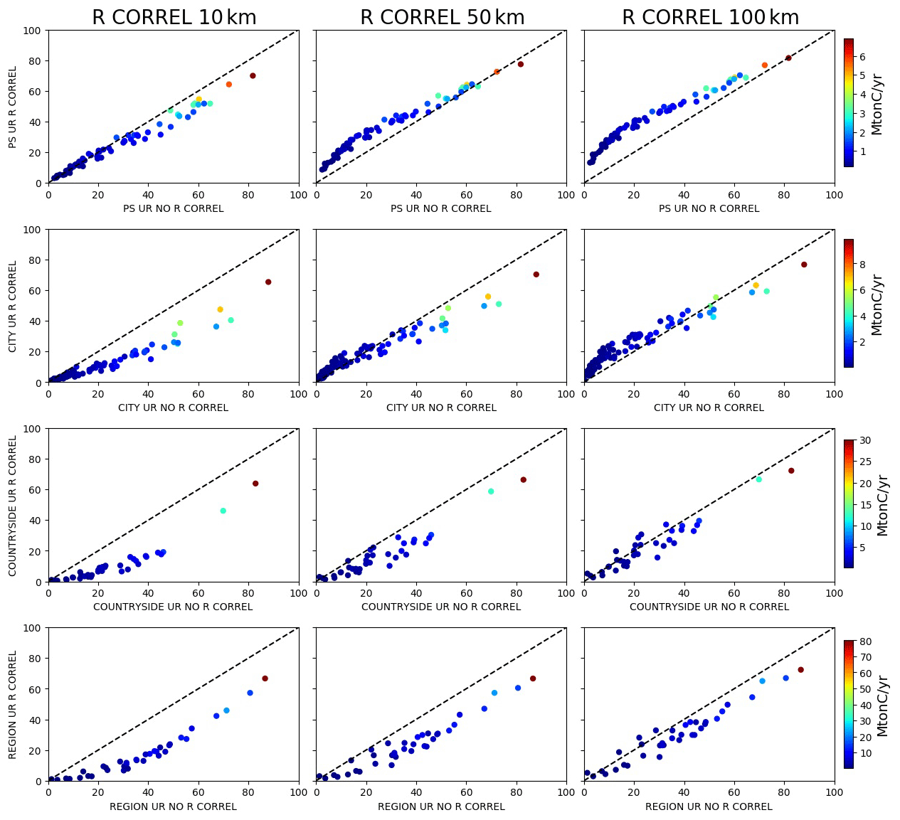
Figure A3 Uncertainty reductions (UR) for the emissions of the point sources (first row), the urban areas (second row), the countryside areas (third row) and the regions (fourth row) when considering spatial correlations (y axis) or no correlations (x axis) between the observation errors. The first, second and third columns correspond to correlations with a spatial scale of 10, 50 and 100 km, respectively. The colors of the dots correspond to the annual budgets of the sources (color bar on the right of the figure). The dashed line is the 1:1 line.

Figure A4 XCO₂ distributions produced by the emissions of the Paris area between 05:00 and 11:00 LT on 8 March at 11:00 LT: raw CHIMERE simulations (a), raw CHIMERE simulations perturbed by an uncorrelated random noise of 0.6 ppm (b), and raw CHIMERE simulations perturbed by a multivariate normal distribution whose covariance matrix is characterized by an uncertainty of 0.6 ppm for the diagonal terms and a correlation length scale of 10 km (c) and of 100 km (d).

These insights into the impact of spatial correlations in R call for further investigations. In particular, we should test more complex patterns that could better correspond to actual model and systematic retrieval errors (e.g., following surface and atmospheric structures). We should also challenge the potential of the inversion to separate such structured observation errors from flux atmospheric signatures under conditions where this inversion is not perfectly informed about the error spatial correlations.