First high-resolution tropospheric NO₂ observations from the Ultraviolet Visible Hyperspectral Imaging Spectrometer (UVHIS)

We present a novel airborne imaging differential optical absorption spectroscopy (DOAS) instrument: the Ultraviolet Visible Hyperspectral Imaging Spectrometer (UVHIS), which is developed for trace gas monitoring and pollution mapping. Within a broad spectral range of 200 to 500 nm and operating in three channels, the spectral resolution of UVHIS is better than 0.5 nm. The optical design of each channel comprises a fore-optics with a field of view (FOV) of 40^∘, an Offner imaging spectrometer and a charge-coupled device (CCD) array detector of 1032×1072 pixels. A first demonstration flight using UVHIS was conducted on 23 June 2018, above an area of approximately 600 km² in Feicheng, China, with a spatial resolution of about 25 m×22 m. Measurements of nadir backscattered solar radiation of channel 3 are used to retrieve tropospheric vertical column densities (VCDs) of NO₂ with a mean total error of 3.0×10¹⁵ molec cm⁻². The UVHIS instrument clearly detected several emission plumes transporting from south to north, with a peak value of 3×10¹⁶ molec cm⁻² in the dominant one. The UVHIS NO₂ vertical columns are consistent with the ground-based mobile DOAS observations, with a correlation coefficient of 0.65 for all co-located measurements, a correlation coefficient of 0.86 for the co-located measurements that only circled the steel factory and a slight underestimation for the polluted observations. This study demonstrates the capability of UVHIS for NO₂ local emission and transmission monitoring.

1 Introduction

Nitrogen oxides (NO_x), the sum of nitrogen monoxide (NO) and nitrogen dioxide (NO₂), play a key role in the chemistry of the atmosphere, such as the ozone destruction in the stratosphere (Solomon, 1999), and the secondary aerosol formation in the troposphere (Seinfeld and Pandis, 2016). In the troposphere, despite lightning, soil emissions and other natural processes, the main sources of NO_x are anthropogenic activities like fossil fuel combustion by power plants, factories and road transportation, especially in urban and polluted regions. As an indicator of anthropogenic pollution which leads to negative effects both on the environment and human health, the amounts and spatial distributions of NO_x have attracted significant attention. For example, China has become one of the largest NO_x emitters in the world due to its fast industrialisation; meanwhile, China has also experienced a series of severe air pollution problems in recent years (Crippa et al., 2018; An et al., 2019). Therefore, measuring the NO_x distribution by applying different techniques would benefit the pollutant emission detection and the air quality trend forecast (Liu et al., 2017; Zhang et al., 2019).

Table 1 UVHIS instrument characteristics of three channels.

Compared to NO, nitrogen dioxide (NO₂) is more stable in the atmosphere. Based on the characteristic absorption structures of NO₂ in the ultraviolet–visible spectral range, the differential optical absorption spectroscopy (DOAS) technique has been applied to retrieve light path integrated densities from different platforms (Platt and Stutz, 2008). Combined the imaging spectroscopy technique, imaging DOAS instruments were developed in recent years to determine the temporal variation and the two-dimensional distribution of trace gases. The global horizontal distribution of tropospheric NO₂ and other trace gases has been mapped and studied by several space-borne sensors, including SCIAMACHY (Scanning Imaging Absorption Spectrometer for Atmospheric CHartographY; Bovensmann et al., 1999), GOME (Global Ozone Monitoring Experiment; Burrows et al., 1999), GOME-2 (Munro et al., 2016), OMI (Ozone Monitoring Instrument; Levelt et al., 2006) and TROPOMI (TROpospheric Ozone Monitoring Instrument; Veefkind et al., 2012). The Environmental trace gases Monitoring Instrument (EMI; Zhao et al., 2018; Cheng et al., 2019; Zhang et al., 2020), as the first designed space-borne trace gas sensor in China, was launched on 9 May 2018, aboard the Chinese GaoFen-5 (GF5) satellite. The spatial resolution of most space-borne sensors is coarser than 10 km×10 km, except for that of TROPOMI, which is 3.5 km×5.5 km.

To achieve a spatial resolution higher than 100 m×100 m for investigating the spatial distribution in urban areas and individual source emissions, several researchers have applied imaging DOAS instruments on airborne platforms. The airborne imaging DOAS measurement was first performed by Heue et al. (2008) over the South African Highveld plateau. To retrieve urban NO₂ horizontal distribution, Popp et al. (2012), General et al. (2014), Schönhardt et al. (2015), Lawrence et al. (2015), Nowlan et al. (2016) and Lamsal et al. (2017), respectively, took measurements in Zürich, Switzerland; Indianapolis and Utqiaġvik (formerly Barrow), USA; Ibbenbüren, Germany; Leicester, England; Houston, USA; and Maryland and Washington DC, USA. In 2013, an airborne measurement focusing on source emissions was taken in China, over Tianjin, Tangshan and the Bohai Bay (Liu et al., 2015). An intercomparison study of four airborne imaging DOAS instruments over Berlin, Germany, suggests a good agreement between different sensors and the effectiveness of imaging DOAS in revealing the fine-scale horizontal variability in tropospheric NO₂ in urban context (Tack et al., 2019).

Here, we present a novel airborne imaging DOAS instrument: the Ultraviolet Visible Hyperspectral Imaging Spectrometer (UVHIS), which was designed and developed by Anhui Institute of Optics and Fine Mechanics, Chinese Academy of Sciences (AIOFM, CAS). As a hyperspectral imaging sensor with a high spectral and spatial resolution, UVHIS is designed for operation on an aircraft platform for atmospheric trace gas measurements and pollution monitoring over large areas in a relative short time frame. By using the DOAS technique and georeferencing, the two-dimensional spatial distribution of tropospheric NO₂ of its first demonstration flight over Feicheng, China, is also presented in this paper.

This paper is organised as follows: Sect. 2 presents a technical description of the UVHIS system and its preflight calibration results. Section 3 introduces the detailed information of its first research flight over Feicheng, China. Section 4 describes the developed algorithm for the retrieval and geographical mapping of tropospheric NO₂ vertical column densities from hyperspectral data. Section 5 presents the retrieved NO₂ column densities, and Sect. 6 compares the airborne measurements with the correlative ground-based data sets from a mobile DOAS system.

2 Instrument details

2.1 UVHIS instrument

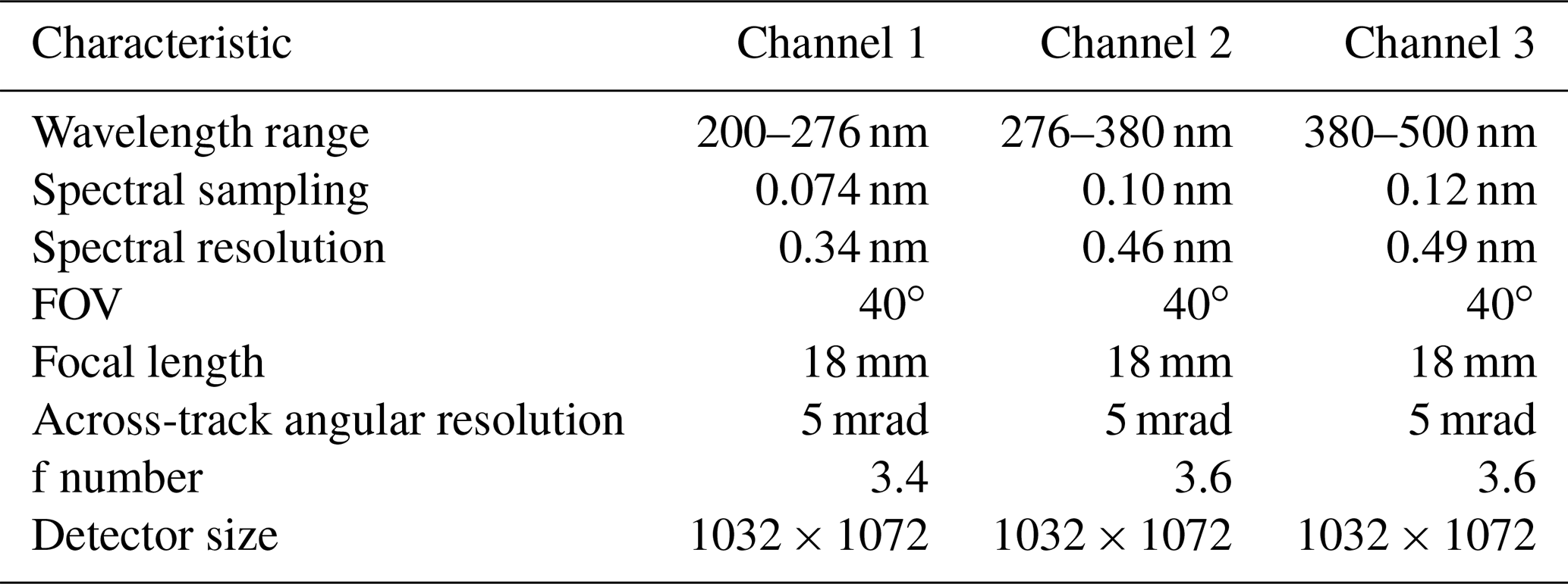
UVHIS is a hyperspectral instrument measuring nadir backscattered solar radiation in the ultraviolet and visible wavelength region from 200 to 500 nm. The instrument is operated in three channels with the wavelength ranges of 200–276 nm (channel 1), 276–380 nm (channel 2) and 380–500 nm (channel 3) for minimal stray light effects and highest spectral performance. The main characteristics of UVHIS are summarised in Table 1.

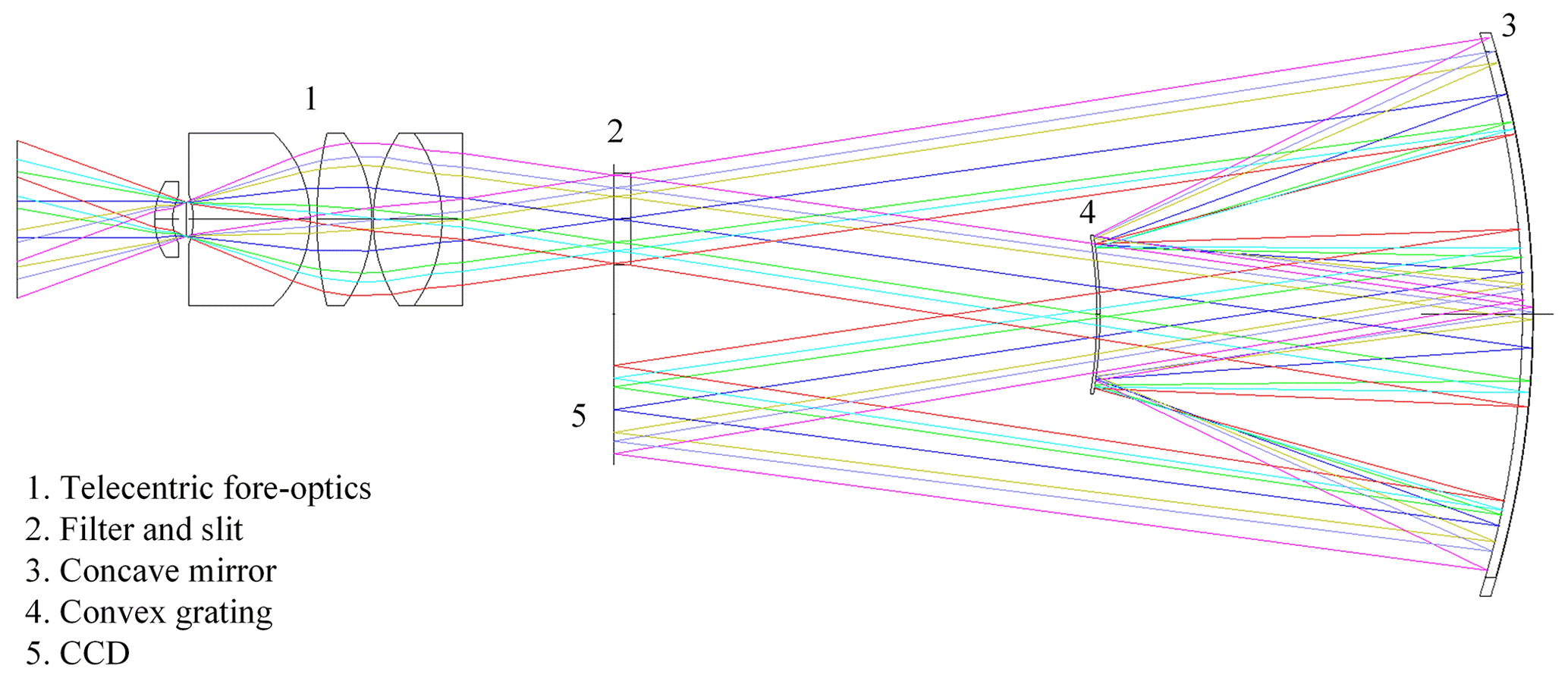
Figure 1 Optical layout of UVHIS channel 3. The optical design of channel 1 and channel 2 is similar.

Figure 1 shows the optical bench of channel 3, and those of the other two are similar. The optical design of each channel comprises a telecentric fore-optics, an Offner imaging spectrometer and a two-dimensional charge-coupled device (CCD) array detector. The Offner imaging spectrometer consists of a concave mirror and a convex grating. The backscattered light below the aircraft is collected by a wide-field telescope with a field of view (FOV) of 40^∘ in the across-track dimension. After passing through a bandpass filter and a 12.5 mm long entrance slit in the focal plane, the light is reflected and diffracted by a concave mirror and a convex grating. The dispersed light is imaged onto a frame transfer CCD detector which consists of 1032×1072 individual pixels. For the alignment and slight adjustment of the spectrometer, only the central 1000 rows of pixels are well illuminated in the across-track dimension. In the wavelength dimension, the image covers the central 1024 columns of pixels on the CCD detector, whilst the left and right edges are used to monitor dark current. The spectral sampling and spectral resolution of all three channels can be found in Table 1.

To reduce dark current and improve the signal-to-noise ratio (SNR) of the instrument, the CCD detector is thermally stabilised at −20 ^∘C with a temperature stability of ±0.05 ^∘C (Zhang et al., 2017). However, the optical bench is not thermally controlled, because the instrument is mounted inside the aircraft platform which has a constant temperature of 20 ^∘C. The UVHIS is mounted on a Leica PAV-80 gyro-stabilised platform that provides angular motion compensation. A high-grade Applanix navigation system on board is used to receive position (i.e. latitude, longitude and elevation) and orientation (i.e. pitch, roll and heading) information, which is required for accurate georeferencing. The UVHIS instrument telescope collects the solar radiation backscattered from the surface and atmosphere through a fused silica window at the bottom of the aircraft. In the case of NO₂ measurement, all observations in this study only use channel 3.

2.2 Preflight calibration

Spectral and radiometric calibration was performed in the laboratory prior to the flights to reduce errors in spectral analysis.

For radiometric calibration, we used an integrating sphere with a tungsten halogen lamp for channel 2 and channel 3. For channel 1, a diffuser plate with a Newport xenon lamp was used for sufficient ultraviolet output. With the help of a well-calibrated spectral radiometer to monitor the radiance of calibration system, the digital numbers from the CCD detectors of the three channels can be converted to radiance correctly. The uncertainty of absolute radiance calibration of the UVHIS is 4.89 % for channel 1, 4.67 % for channel 2 and 4.42 % for channel 3.

Table 2 Preflight wavelength calibration results (full width at half maximum values; FWHMs) of UVHIS channel 3 for nine viewing angles. Light sources used in the calibration are a mercury–argon lamp and a tuneable laser. Slit function shapes are retrieved by least square fitting of characteristic spectral lines, using a symmetric Gaussian function.

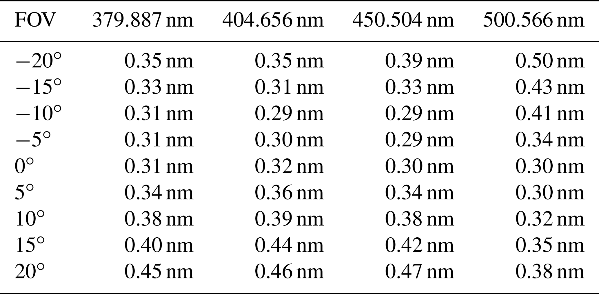
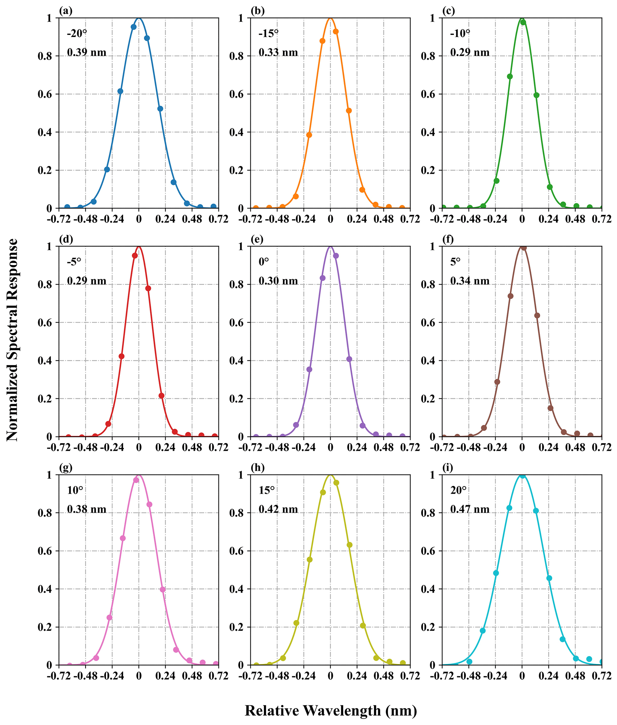
Figure 2 Measured slit functions (dots) at 450.504 nm and retrieved slit function shapes (lines) using a symmetric Gaussian function for nine viewing angles.

Preflight wavelength calibration was also performed in the laboratory, using a mercury–argon lamp and a tuneable laser as light sources. We modelled the slit function of the UVHIS using a symmetric Gaussian function. Spectral registration and slit function calibration were achieved by least square fitting of the characteristic lines in the collected spectra. Table 2 lists the retrieved full width at half maximum values (FWHMs) for channel 3. Figure 2 shows the measured slit functions at 450.504 nm for nine viewing angles (i.e. −20, −15, −10, −5, 0, 5, 10, 15, 20^∘) and the respective retrieved slit function shapes using a symmetric Gaussian function. These Gaussian fit results suggest that a symmetric Gaussian function is a reasonable assumption for the slit shape in all viewing directions.

3 Research flight

The first demonstration flight over the city of Feicheng, the town of Shiheng and neighbouring rural areas was conducted on 23 June 2018, aiming at producing tropospheric NO₂ field maps of a large area in a relatively short time frame. Feicheng is a county-level city in the Shandong province, approximately 410 km away from Beijing. Figure 3 shows the TROPOMI NO₂ tropospheric observation on 23 June 2018, with the background Google map and the location of Feicheng. The flight area is located on the south bank of the Yellow River, at the western foot of Mount Tai. The UVHIS was operated from the Y-5 aircraft at an altitude of 3 km a.s.l., which is higher than the height of planetary boundary layer (PBL), with an average aircraft ground speed of 50 m s⁻¹. An overview of the observation area and the flight lines is provided in Fig. 4. The aircraft took off at local noon from the airfield in Pingyin County, approximately 19 km northwest of the centre of the field. An area of approximately 600 km² was covered in 3 h, under clean sunny and cloudless conditions with low-speed southerly winds.

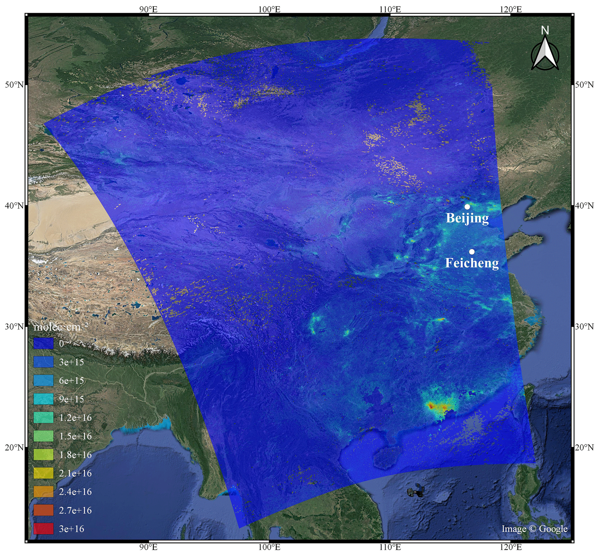
Figure 3 TROPOMI observation of tropospheric NO₂ over China on 23 June 2018. The location of the UVHIS flight (Feicheng city) is also plotted in the map.

Figure 4 Overview of the Feicheng demonstration flight on 23 June 2018. Flight lines are shown in blue. Two orange circles represent the routes of the mobile DOAS system. White dots numbered from 1 to 8 represent the major emission sources. Number 1: several carbon factories; number 2: a power plant; numbers 3–6: individual emitters inside the steel factories, while numbers 4 and 5 are inside the circle of one mobile DOAS route; numbers 7–8: two cement factories. The dashed white box represents the reference area.

The research flight included 13 parallel lines in the east–west direction, starting from the lower left corner in Fig. 4. The distance between adjacent lines was 1.5 km, whilst the swath width of each individual line was approximately 2.2 km. Gapless coverage between adjacent lines can be guaranteed in this pattern because of the adequate overlap. To validate the NO₂ column densities retrieved from the UVHIS by comparison to ground measurements, mobile DOAS measurements were taken inside the research area on the same day. As shown in Fig. 4, the measurements of the mobile DOAS system circled around the steel factory and the power plant which are the presumed major emission sources inside the observation area.

4 Data processing chain

The NO₂ tropospheric vertical column density (VCD) retrieval algorithm of the UVHIS consists of four major steps. First, some necessary pre-processing procedures are required before any spectral analysis of the UVHIS data. Next, the UVHIS spectral data after pre-processing are analysed in a suitable wavelength region by applying the well-established DOAS technique. Then, the air mass factors (AMFs) are calculated for every observation based on the SCIATRAN radiative transfer model to convert the slant column densities (SCDs) to tropospheric vertical column densities. In the final step, the georeferenced NO₂ VCDs are resampled and overlaid onto Google satellite map layers.

4.1 Pre-processing

The pre-processing procedure before spectral analysis includes data selection, georeferencing, dark current correction, spatial binning and in-flight calibration. First, the spectral data acquired during aircraft U turns are removed in the processing because of the large and changing orientation angles. Furthermore, a radiance threshold of 12.8 $\mathrm{\mu }\mathrm{W}{\mathrm{cm}}^{-\mathrm{2}}{\mathrm{sr}}^{-\mathrm{1}}{\mathrm{nm}}^{-\mathrm{1}}$ at 450 nm is set to neglect some over-illuminated ground pixels inside the flight area, which are usually caused by the presence of clouds or water mirror reflection. During the entire flight, the Sun glinted on water several times in the southern part of the flight area, especially above the river near the reference area. However, clouds were not present due to the clean clear-sky weather condition.

Accurate georeferencing is essential for emission source locating and data comparison, and can be achieved with the sensor position and orientation information recorded by the navigation system and inertial measurement unit (IMU) on board.

Dark current correction is performed based on the measurement at the start of the entire flight by blocking the fore-optics, which is necessary to improve the instrument performance and reduce the analysis error in DOAS fit.

In order to increase the SNR of the instrument and the sensitivity to NO₂, the raw pixels of the imaging DOAS are usually aggregated in the across- and along-track directions. According to photon statistics when only shot noise is considered, the SNR should rise with the square root of the number of binned spectra. However, this improved SNR of the instrument results in reduced spatial resolution. In the data analysis of the Feicheng flight, we use the binning of 10 pixels in the across-track direction, resulting in a ground pixel size of approximately 25 m×22 m.

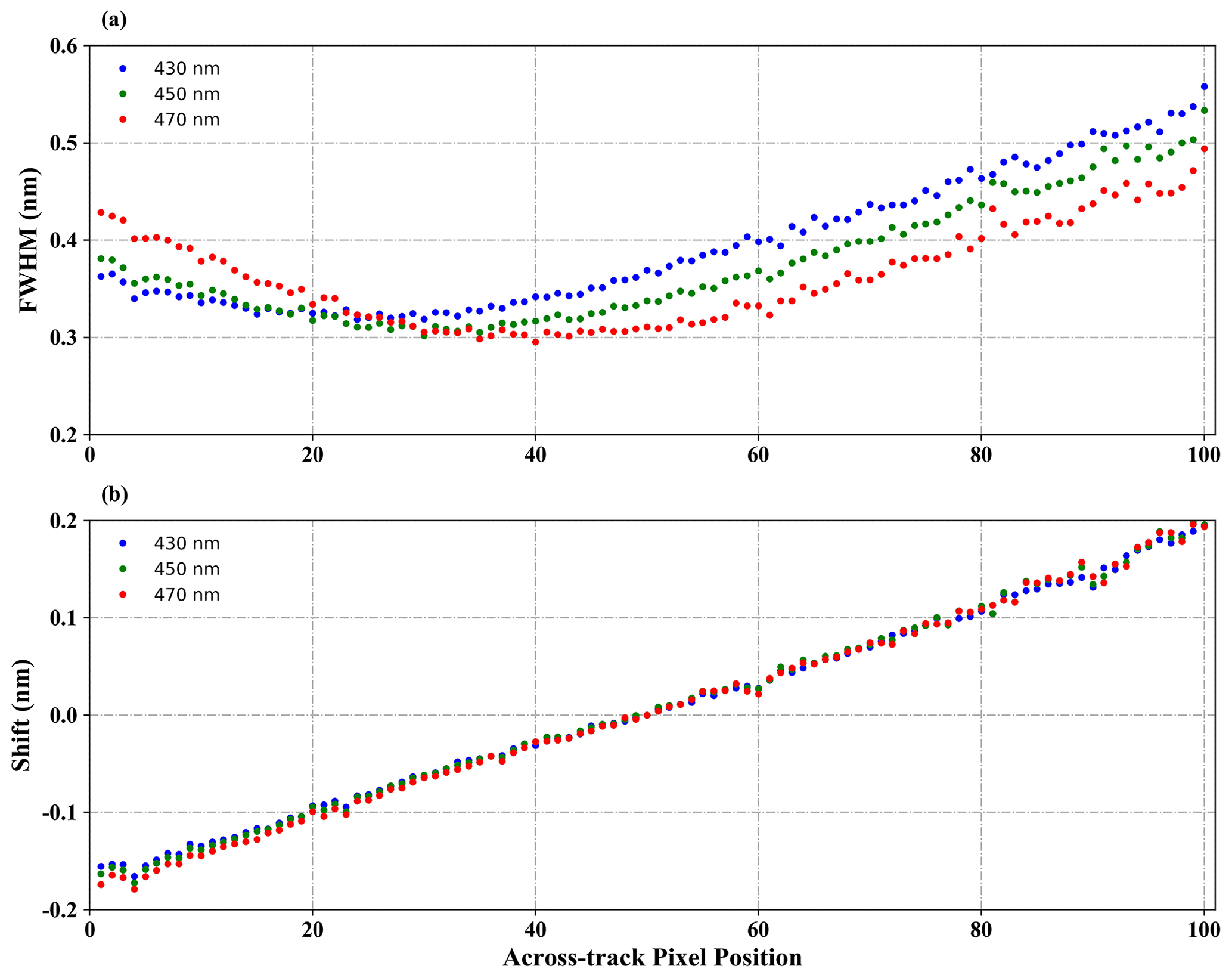
Figure 5 In-flight spectral calibration: (a) the spectral resolution (FWHM); (b) the spectral shift on different across-track positions. Results at three wavelengths are plotted: blue for 430 nm, green for 450 nm and red for 470 nm.

Given that the wavelength-to-pixel registration and the slit function shape of the UVHIS could change compared to laboratory calibration results, in-flight wavelength calibration is essential for the next DOAS analysis. This in-flight wavelength calibration is achieved by fitting the measured spectra to a high-resolution solar reference (Chance and Kurucz, 2010) with slit function convolution and wavelength shift. The nominal wavelength-to-pixel registration determined in laboratory calibration is used as initial values in the iteratively fitting procedure for convergence to the optimal solution. The effective shifts and FWHMs of different across-track positions are plotted in Fig. 5. The results at three wavelengths are presented as follows: blue for 430 nm (the start of the analysis wavelength region), green for 450 nm (the middle of the analysis wavelength region) and red for 470 nm (the end of the analysis wavelength region).

4.2 DOAS analysis

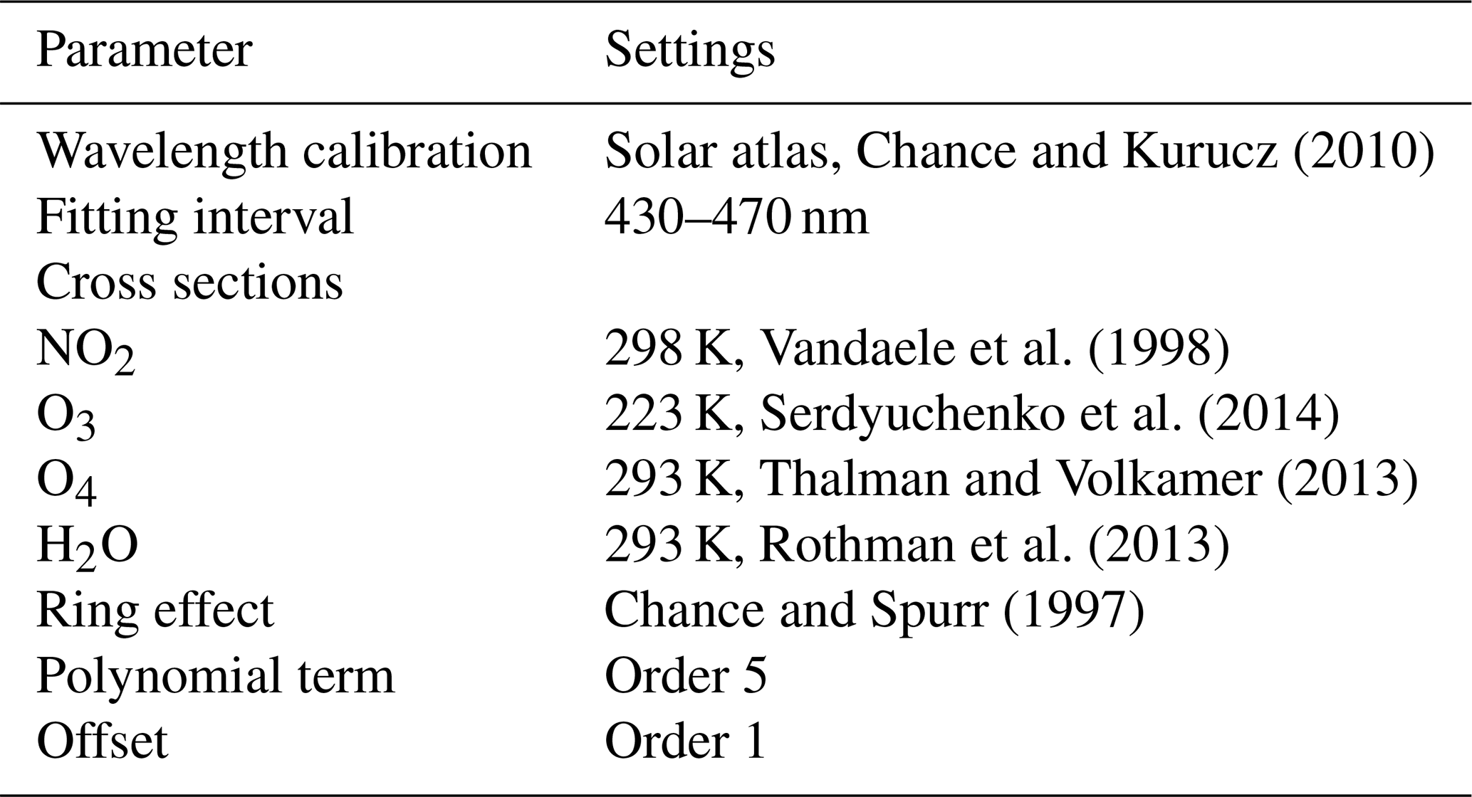
After pre-processing, the observed UVHIS spectra are analysed using the QDOAS software (Danckaert et al., 2020) to retrieve the NO₂ slant column densities. The basic idea of the DOAS approach is to separate broadband signals like surface reflectance and Rayleigh scattering, and narrow-band signals like trace gas molecular absorption. The fit window is 430–470 nm, which is considered to contain strongly structured NO₂ absorption features and with low interference of other trace gases such as O₃, O₄ and water vapour. The absorption cross sections of NO₂ and other trace gases and a synthetic Ring spectrum are simultaneously fitted to the logarithm of the ratio of the observed spectrum to the reference spectrum. These cross sections are made by convolving the high-resolution cross sections with the in-flight wavelength calibration results for all across-track positions. Further details of the DOAS analysis setting can be found in Table 3.

Table 3 Main analysis parameters and absorption cross sections for NO₂ DOAS retrieval.

For each analysed spectrum, the direct result of the DOAS fit is the differential slant column density (dSCD), which is the NO₂ integrated concentration difference along the effective light path between the studied spectrum and the selected reference spectrum (SCD_ref). Reference spectra were acquired over a clean rural area upwind of the urban and factory areas, as shown in the lower left corner of Fig. 4. In the quite homogeneous background area, several spectra were averaged to increase the SNR of the reference spectrum. To avoid across-track biases, a reference spectrum is required for each across-track position because of its intrinsic spectral response. According to the TROPOMI tropospheric NO₂ product of the reference area on the same day, the residual NO₂ amount in the background spectra is estimated to be 3×10¹⁵ molec cm⁻². Changes in the stratospheric NO₂ could also propagate to the measured tropospheric columns of UVHIS. Under the assumption of a constant stratosphere in time and space during the flight, the changes in the solar zenith angle (SZA) impact the column difference between the measurement and the reference. To correct the change in the stratospheric NO₂ SCD, we apply a geometric approximation of the stratospheric AMF with a stratospheric VCD of 3.5×10¹⁵ molec cm⁻² from TROPOMI product. The maximum change in the stratospheric SCD with respect to the reference was 8×10¹⁴ molec cm⁻².

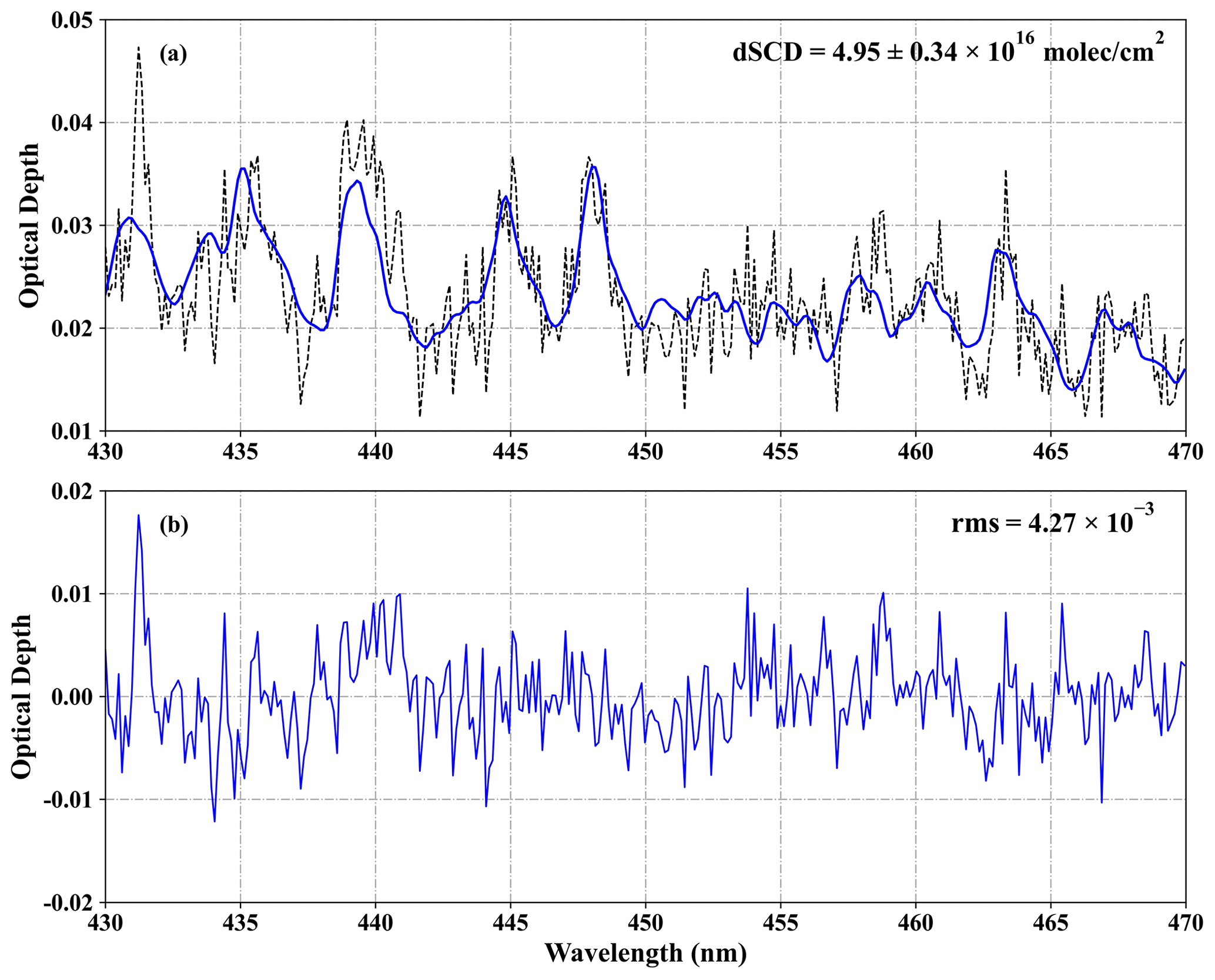
Figure 6 Sample DOAS fit result for NO₂: (a) observed (dashed black line) and fitted (blue line) optical depths from measured spectra; (b) the remaining residuals of DOAS fit.

A sample NO₂ DOAS fit result and the corresponding residual of UVHIS spectra are illustrated in Fig. 6 with a dSCD of $\mathrm{4.95}\pm \mathrm{0.34}\times {\mathrm{10}}^{\mathrm{16}}$ molec cm⁻² and a rms on the residuals of $\mathrm{4.27}\times {\mathrm{10}}^{-\mathrm{3}}$.

4.3 Air mass factor calculations

SCD is the integrated concentration along the effective light path of observation, which is strongly dependent on the viewing geometry and the properties that influence radiative transfer of light through the atmosphere. VCD is the integrated concentration along a single vertical transect from the Earth's surface to the top of the atmosphere, which is independent of the changes in the light path length of the SCD.

$$\begin{array}{ll}{\displaystyle }{\mathrm{VCD}}_i^{\mathrm{t}}& {\displaystyle }={\displaystyle \frac{{\mathrm{dSCD}}_i+{\mathrm{dSCD}}_i^{\mathrm{s}}+{\mathrm{SCD}}_{\mathrm{ref}}^{\mathrm{t}}}{{\mathrm{AMF}}_i^{\mathrm{t}}}}\\ \text{(1)}& {\displaystyle }& {\displaystyle }={\displaystyle \frac{{\mathrm{dSCD}}_i+{\mathrm{dSCD}}_i^{\mathrm{s}}+{\mathrm{VCD}}_{\mathrm{ref}}^{\mathrm{t}}\times {\mathrm{AMF}}_{\mathrm{ref}}^{\mathrm{t}}}{{\mathrm{AMF}}_i^{\mathrm{t}}}}\end{array}$$

As shown in Eq. (1), the dSCD_i from the DOAS fit can be converted to tropospheric ${\mathrm{VCD}}_i^{\mathrm{t}}$ by dividing the ${\mathrm{AMF}}_i^{\mathrm{t}}$ which accounts for the enhancements in the light path (Solomon et al., 1987). The ${\mathrm{dSCD}}_i^{\mathrm{s}}$ is the stratospheric SCD difference between the measurement and the reference; the ${\mathrm{SCD}}_{\mathrm{ref}}^{\mathrm{t}}$, the ${\mathrm{VCD}}_{\mathrm{ref}}^{\mathrm{t}}$ and the ${\mathrm{AMF}}_{\mathrm{ref}}^{\mathrm{t}}$ are the tropospheric SCD, VCD and AMF of the reference. In this study, tropospheric NO₂ AMFs have been computed using the SCIATRAN (Rozanov et al., 2014) radiative transfer model (RTM). The SCIATRAN model numerically calculates AMFs based on a priori information on the parameters that changes the effective light path, such as Sun and viewing geometry, trace gas and aerosol vertical profiles and surface reflectance.

4.3.1 Parameters in RTM

(1) During flight, the viewing geometry is retrieved from the orientation information of the aircraft. The solar position defined by the SZA and the solar azimuth angle (SAA), as well as the relative azimuth angle (RAA), can be calculated based on the time information and the latitude and longitude position of each observation. (2) Since the flight is performed under a clear-sky condition, the effect of cloud presence can be ignored in AMF computation. (3) The surface reflectance used in AMF calculation is the product of the Landsat 8 Operational Land Imager (OLI) space-borne instrument (Barsi et al., 2014). The coastal aerosol band (433 to 450 nm) is selected because its bandwidth is relatively narrow, and this band is basically inside the DOAS fitting window (Vermote et al., 2016). (4) Since no accurate trace gas vertical profile is available during flight, a well-mixed vertical distribution (box profile) of NO₂ in the PBL is assumed. However, accurate PBL height is also unavailable, so the typical height of 2 km is a reasonable guess on a sunny summer day in the midlatitude area in China. (5) The aerosol optical depth (AOD) information used in AMF calculation is the MODIS AOD product MYD04 at 470 nm on the same day with resampling for every ground UVHIS pixel (Remer et al., 2005), because ground-based aerosol measurement is not performed and no Aerosol Robotic Network (AERONET) station data near the flight area are available. The MODIS AOD measurements inside the flight area range from 0.14 to 0.36. Like the NO₂ profile, the aerosol extinction box profile is constructed from the PBL height and the AOD. A single scattering albedo (SSA) is assumed to be 0.93, and an asymmetry factor is assumed to be 0.68 for the aerosol extinction profile, based on previous studies of typical urban/industrial aerosols (Li et al., 2018).

The Landsat 8 surface reflectance is retrieved through atmospheric correction, using the Second Simulation of the Satellite Signal in the Solar Spectrum Vectorial (6SV) model (Vermote et al., 1997). Since no overpass on the same day existed inside the UVHIS research flight area, we selected the surface reflectance product on 3 May 2018, considering the sunny weather conditions and no cloud presence. The spatial resolution of Landsat is approximately 30 m, which is slightly larger than that of the UVHIS. A resampling of the Landsat 8 surface reflectance product based on nearest neighbour interpolation was performed for every UVHIS ground pixel.

Table 4 Overview of the input parameters in the SCIATRAN RTM, characterising the AMF LUT.

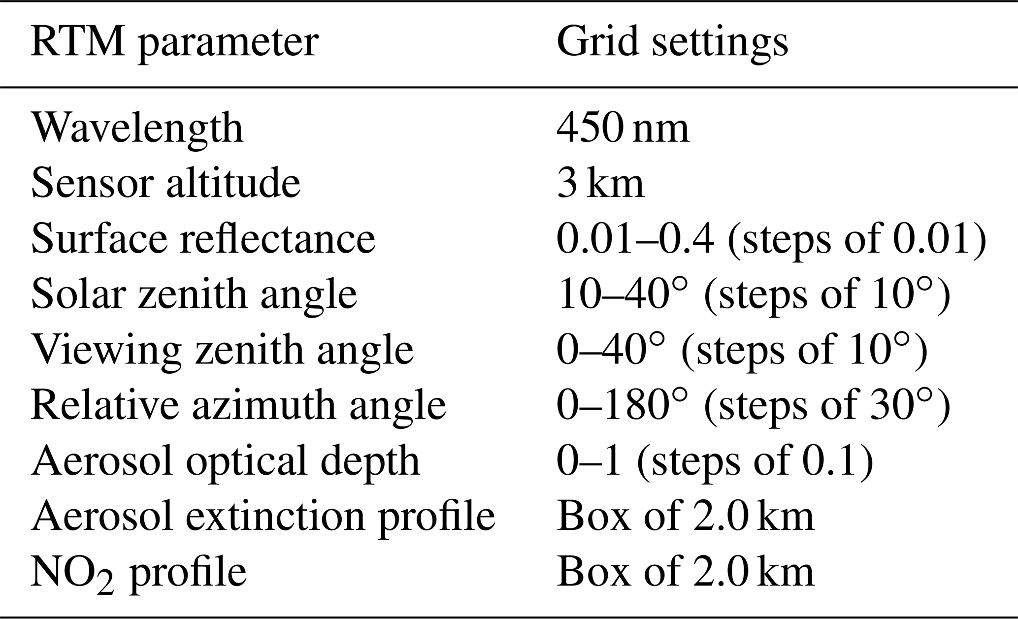
The radiative transfer equation in SCIATRAN is solved in a pseudo-spherical multiple scattering atmosphere, using the scalar discrete ordinate technique. Simulations were performed for the sensor altitude of 3 km a.s.l. and the wavelength of the middle of the NO₂ fitting windows, i.e. 450 nm. A NO₂ AMF look-up table (LUT) was computed, with the different RTM parameter settings provided in Table 4. For each retrieved dSCD, an AMF was linearly interpolated from the LUT based on the Sun geometry, the viewing geometry and the surface reflectance.

4.3.2 RTM dependence study

AMF dependence on the surface reflectance

As shown in Fig. 7, a time series of computed AMFs is plotted for the research flight on 23 June 2018, as well as the corresponding surface reflectance, solar zenith angles and relative azimuth angles. Note that only data of nadir observations are plotted for a clear display, and the time gaps between adjacent flight lines can be observed. Despite the great degree of varieties in viewing and Sun geometries, the AMFs strongly depend on the surface reflectance. Previous studies reported by Lawrence et al. (2015), Meier et al. (2017) and Tack et al. (2017) suggest a similar conclusion. A sensitivity test was carried out to investigate the impact of surface reflectance on the AMF calculations based on the SCIATRAN model, with varying values of surface reflectance and the fixed values of other parameters. The results of this test are shown in Fig. 8a and indicate that the relation between the surface reflectance and the AMF is non-linear. Especially when the surface reflectance is below 0.1, the AMF increases with the surface reflectance rapidly.

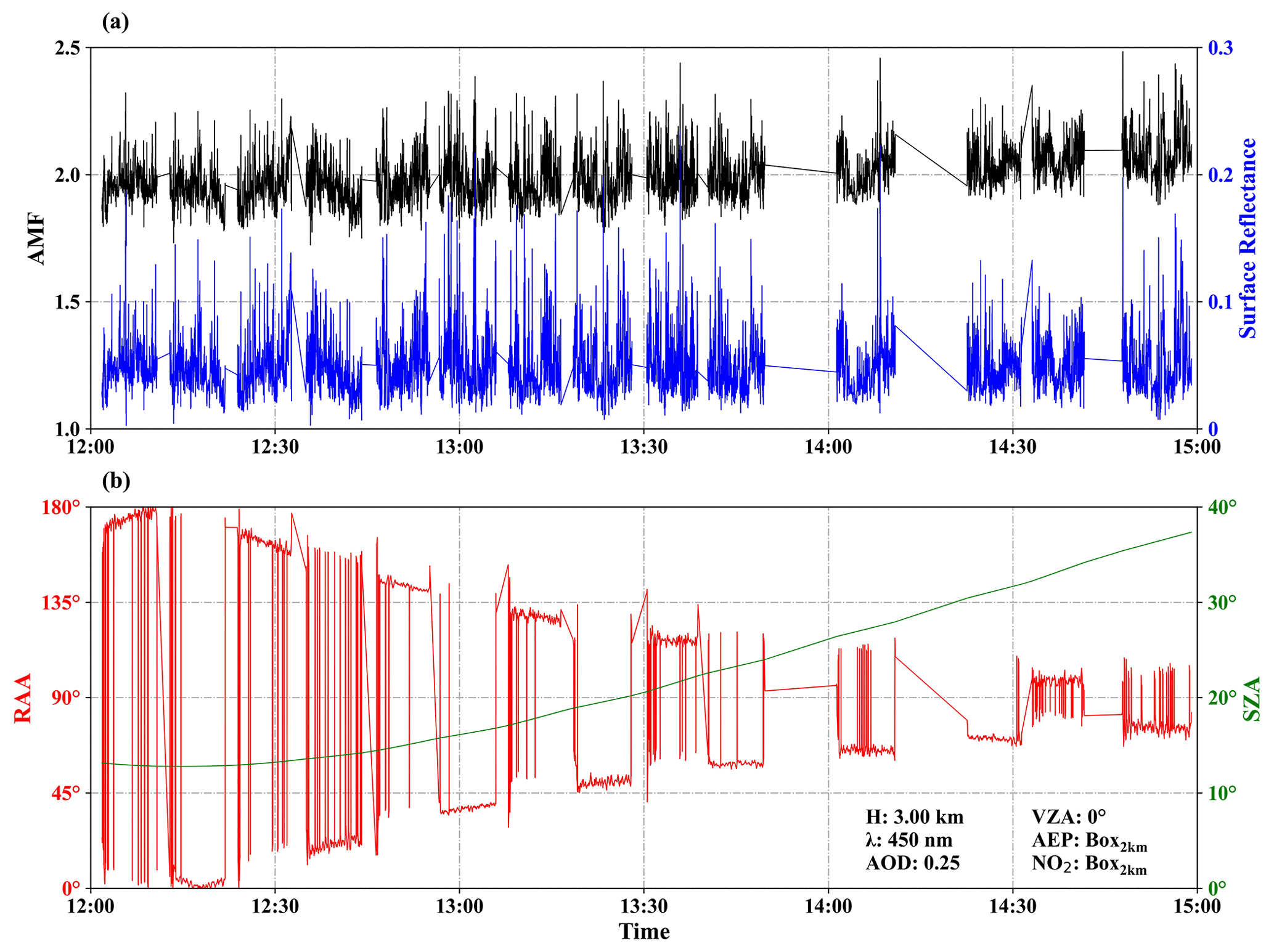
Figure 7 Time series of NO₂ AMF compared with (a) surface reflectance; (b) SZA and RAA for the research flight on 23 June 2018, computed with SCIATRAN model based on the RTM parameters from the UVHIS instrument. Only data of the nadir observations in each flight line are plotted.

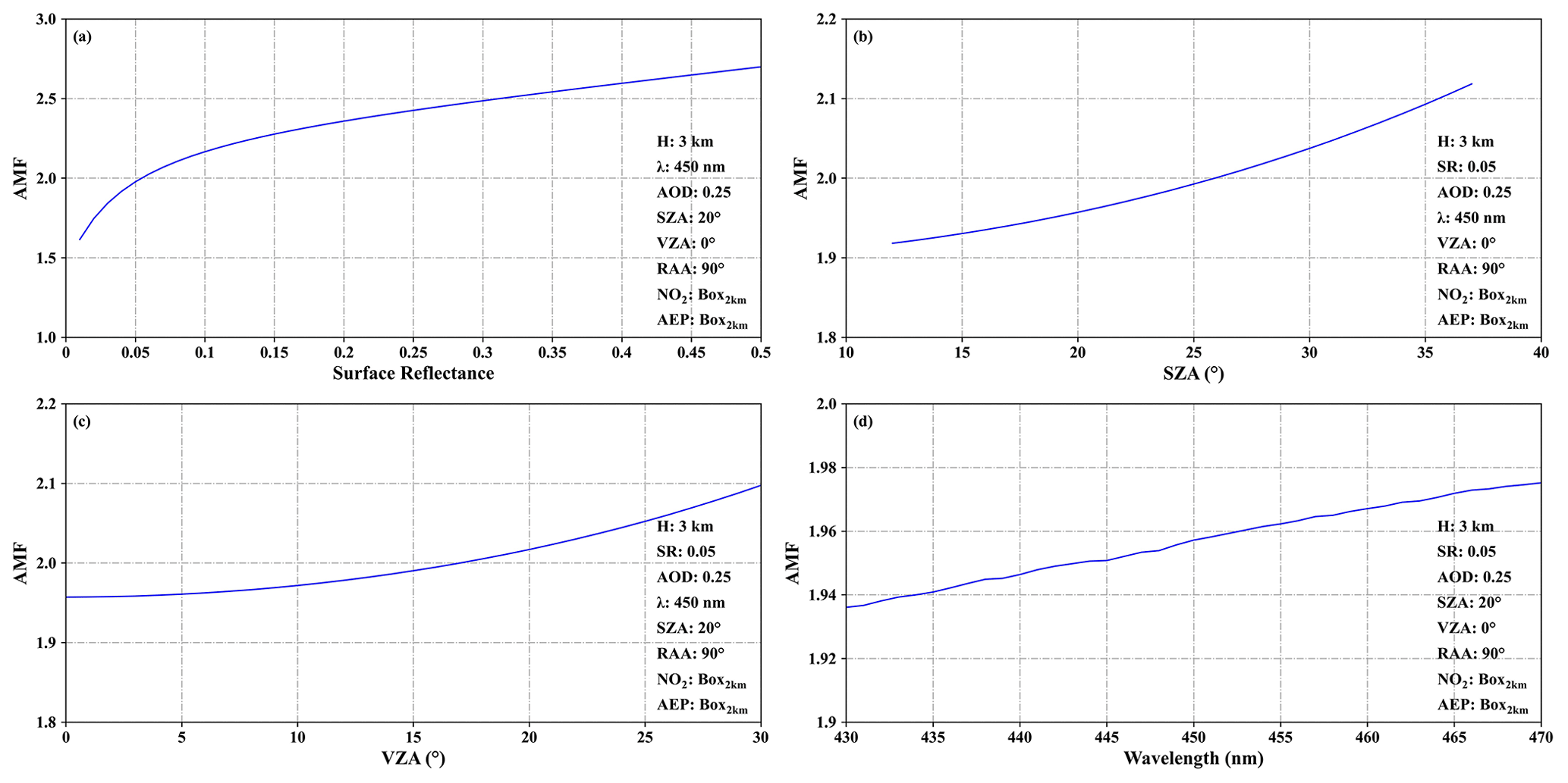
Figure 8 AMF dependence analysis results (a) on the surface reflectance; (b) on the SZAs; (c) on the VZAs; (d) on the wavelength.

Generally speaking, the AMF should be higher in the case of a bright surface reflectance because more sunlight is reflected from the ground back to the atmosphere and then recorded by the airborne sensor. Compared to rural areas, urban and industrial areas usually exhibit enhanced surface reflectance and a subsequent increment in AMF. As shown in Fig. 9, the dependency of the AMF on the surface reflectance is very strong. Moreover, a strong variability of the surface reflectance and the AMF can be observed in these areas. Figure 9 also shows several slight inconsistencies between the UVHIS measured radiance and the Landsat 8 surface reflectance product. For example, the east–west main road looks thinner in Fig. 9a compared to Fig. 9b and c. This could be explained by the relatively higher spatial resolution performance of the UVHIS and the resampling of Landsat 8 pixels.

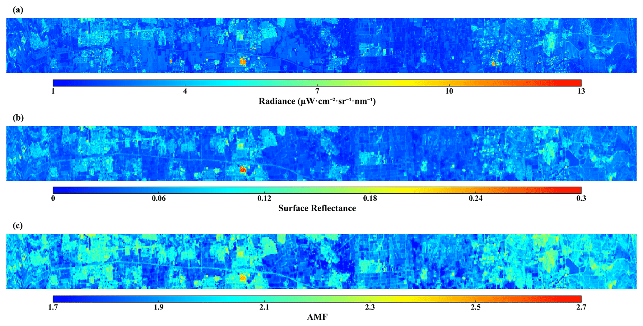
Figure 9 (a) UVHIS measured radiance; (b) Landsat 8 surface reflectance; (c) computed AMFs for one flight line of the Feicheng data set. A strong dependency of the AMF on the surface reflectance can be observed.

AMF dependence on profiles

Based on airborne UVHIS retrieval product, the horizontal distribution of NO₂ can be detected, but the vertical distribution of NO₂ in the atmosphere is unavailable. The assumptions we made for the profile shape of the trace gas and aerosol extinction do not consider the effective variability during research flight which can be expected in an urban area. Focusing on the impact of different profile shapes on the AMF computation, sensitivity tests of two different NO₂ profiles which are closer to ground surface were performed: well-mixed NO₂ box profiles of 0.5 and 1 km heights. Compared to the box profile of 2 km which is near the estimated height of PBL, the AMFs decreased by an average of 13 % in the case of a box profile of 1.0 km, whilst the AMFs decreased by an average of 22 % in the case of a box profile of 0.5 km.

Depending on the relative position of the aerosol and trace gas layer, the optical thickness and the scattering properties, aerosols can enhance or reduce the AMF in different ways (Meier et al., 2017). If an aerosol layer is located above the majority of the trace gas, the aerosols with high SSA have a shielding effect as less scatter light passes through the trace gas layer, leading to a shorter light path. On the other hand, if aerosols and the trace gas are present in the same layer, the aerosols can lead to multiple scattering effects which extend the light path and result in a larger AMF. According to the simulations of a well-mixed aerosol box profile of 2 km and a pure Rayleigh atmosphere, AMFs are slightly higher (by approximately 1 %) than those of the pure Rayleigh scenario.

AMF dependence on Sun and viewing geometries

Figure 7 shows that the effect of Sun and viewing geometries on AMFs is very small. Based on a previous study by Tack et al. (2017), the changing SZA have the greatest effect on the AMFs, compared to other Sun and viewing geometries. In this study, we also performed an AMF dependence analysis on SZAs and viewing zenith angles (VZAs). The SZA varied from 12.8 to 37.4^∘ during the 3 h research flight, whilst the VZA ranged from 0 to 30^∘ in most cases. As shown in Fig. 8b and c, the changes in AMF were less than 10 % and 7 %, respectively, when other parameters were set to the mean values. Generally, a larger SZA or a larger VZA could result in a longer light path through the atmosphere and thus a larger AMF.

AMF dependence on the analysis wavelength

The dependence of AMF on the analysis wavelength is shown in Fig. 8d. The AMF increases with the analysis wavelength. This could be explained by the Rayleigh scattering characteristics. That is, photons at shorter wavelengths are more likely to be scattered than photons at longer wavelengths, leading to reduced sensitivity to AMF at shorter wavelengths. In the DOAS analysis wavelength window of 430–470 nm, the increase in AMF is approximately 2 %.

4.4 Resampling and mapping

The georeferenced NO₂ VCDs are gridded to combine overlapped adjacent measurements, with a spatial resolution of $\mathrm{0.0003}{}^{\circ }\times \mathrm{0.0002}{}^{\circ }$. Corresponding to 27 m×22 m, the grid size used is slightly larger than the effective spatial resolution of the UVHIS to reduce the number of empty grid cells. All VCDs are assigned to a grid cell based on its centre coordinates, and several VCDs in one grid cell are an unweighted average. As shown in Fig. 10, the final NO₂ VCD distribution map is plotted over the satellite maps layers in QGIS 3.8 software (QGIS development team, 2020).

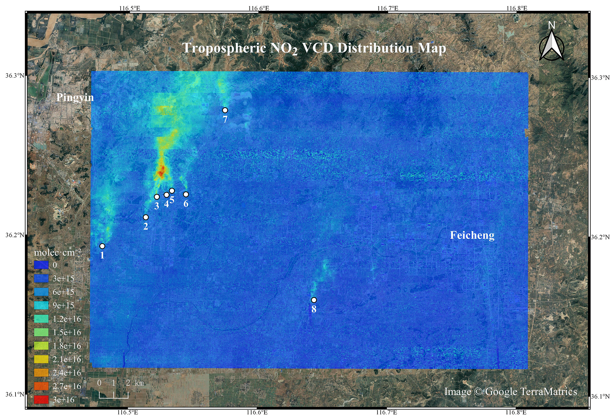
Figure 10 Tropospheric NO₂ VCD map retrieved from UVHIS over Feicheng on 23 June 2018. The major contributing NO_x emission sources are indicated by numbers 1 to 8.

5 Results

The tropospheric NO₂ VCD two-dimensional distribution map is shown in Fig. 10 for the research flight on 23 June 2018. With the high performance of UVHIS in spectral and spatial resolution, Fig. 10 shows fine-scale NO₂ spatial variability to resolve individual emission sources. In general, the NO₂ distribution is dominated by several exhaust plumes with enhanced NO₂ concentration in the northwest part that share a transportation pattern from south to north that is consistent with the wind direction. These sources include a power plant, a steel factory, two cement factories and several carbon factories. The largest plume, with peak values of up to 3×10¹⁶ molec cm⁻², originated from an emitter inside a steel factory (number 3 in Fig. 10). This dominant plume reaches its peak value outside at a small valley approximately 1 km north of the factory and was transporting at least 9 km and seems to be continuing outside the flight region. This enhanced level of NO₂ may be caused by the terrain factor which contributes to the accumulation of pollution gases.

Numbers 4 to 6 represent other emitters inside the steel factory, whilst the exhaust plumes from numbers 4 and 5 merged with the dominant plume, the plume from number 6 transported to north individually with a peak value of 1.4×10¹⁶ molec cm⁻². A plume with peak values of 1.5×10¹⁶ molec cm⁻² was also detected by UVHIS, which seemed to originate from the power plant. Indicated by number 2 in Fig. 10, this power plant is less than 2 km south of the steel factory. Number 1 in Fig. 10 indicates several carbon factories which are located on the left side of the flight area. Several plumes with peak values of 1.6×10¹⁶ molec cm⁻², gradually merged during transportation downwind. Numbers 7 and 8 in Fig. 10 represent two different cement factories. The peak values of these two plumes are 1.5×10¹⁶ and 1.4×10¹⁶ molec cm⁻², respectively.

Compared to the industrial areas mentioned above, the pollution levels of the rural areas are much lower due to the lack of contributing sources, ranging from 2 to 6×10¹⁵ molec cm⁻². The urban area of Feicheng city is located on the right side of the flight area. Figure 11 is an enlarged map of the UVHIS NO₂ observations over Feicheng city, with a colour scale that only extends to 7×10¹⁵ molec cm⁻². The two black lines in Fig. 11 represent the truck roads in this city. S104 is a provincial highway that crosses Feicheng from north to south, whilst S330 crosses Feicheng from east to west.

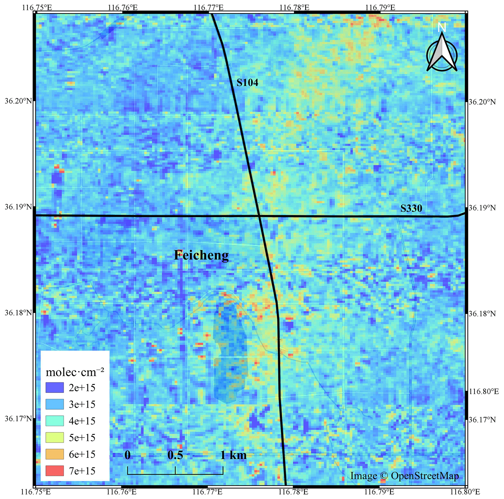
Figure 11 Enlargement of UVHIS NO₂ VCD map over Feicheng city with a colour scale only extends to 7×10¹⁵ molec cm⁻². Two black lines in the map represent two truck roads that cross Feicheng city: S104 and S330. © OpenStreetMap contributors 2021. Distributed under a Creative Commons BY-SA License.

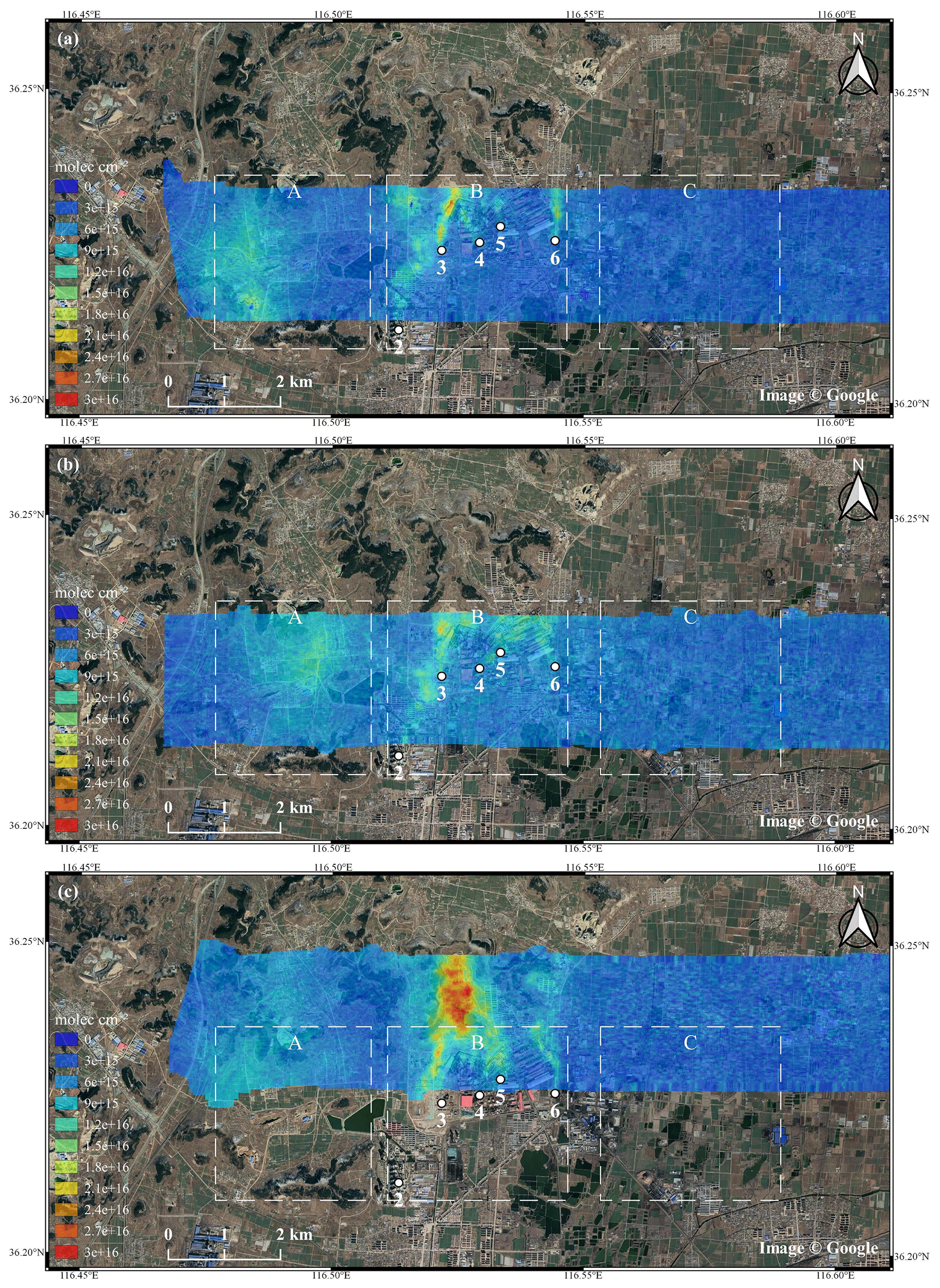
Figure 12 Three flight lines that pass through the steel factory at 13:26 (a), 14:57 (b) and 13:32 LT (c). Panels (a) and (b) represent flight lines that cover the same area with a 1.5 h time gap; (a) and (c) represent adjacent flight lines with a 6 min time gap.

Due to temporal discontinuity of the flight lines and the dynamic characteristics of the tropospheric NO₂ field, artefacts can be observed between adjacent flight lines. Figure 12 shows three flight lines that pass through the steel factory at 13:26 (a), 14:57 (b) and 13:32 LT (c). Figure 12a, b represent the flight lines that cover the same area with a 1.5 h time gap, and Fig. 12a, c represent adjacent flight lines with a 6 min time gap. These flight lines can be divided into three regions: region A covers no NO₂ source but is affected by the carbon factories approximately 3 km away; region B covers the steel factory as the dominant NO₂ source; region C covers no NO₂ source and is not affected by other sources. In these three regions, only region C is temporally consistent with relatively low NO₂ columns, whilst a large temporal variety of NO₂ VCDs exists in region A and region B because of inconstant emission sources and changing meteorology.

6 NO₂ VCD assessment

6.1 Uncertainty analysis

The total uncertainty on the retrieved tropospheric NO₂ VCDs is composed of three parts: (1) uncertainties in the retrieved dSCDs, (2) uncertainties in reference column SCD_ref and (3) uncertainties in computed AMFs. Assuming that these uncertainties originating from independent steps are sufficiently uncorrelated, the total uncertainty of the tropospheric NO₂ VCD can be quantified as follows:

$$\begin{array}{ll}{\displaystyle }& {\displaystyle }{\mathit{\sigma }}_{{\mathrm{VCD}}_i}\\ \text{(2)}& {\displaystyle }& {\displaystyle }=\sqrt{{\left({\displaystyle \frac{{\mathit{\sigma }}_{{\mathrm{dSCD}}_i}}{{\mathrm{AMF}}_i}}\right)}^{\mathrm{2}}+{\left({\displaystyle \frac{{\mathit{\sigma }}_{{\mathrm{SCD}}_{\text{ref}}}}{{\mathrm{AMF}}_i}}\right)}^{\mathrm{2}}+{\left({\displaystyle \frac{{\mathrm{SCD}}_i}{{\mathrm{AMF}}_i^{\mathrm{2}}}}\times {\mathit{\sigma }}_{{\mathrm{AMF}}_i}\right)}^{\mathrm{2}}}.\end{array}$$

The first uncertainty source, ${\mathit{\sigma }}_{{\text{dSCD}}_i}$, originates from the DOAS fit residuals and is a direct output in the QDOAS software. This dSCD uncertainty is dominated by the shot noise from radiance, the electronic noise from the instrument, the systematic uncertainties from the cross sections and the errors from wavelength calibration. In this study, spatial binning of 10 pixels is performed to reduce these DOAS fit residuals, with a mean slant error of 4.8×10¹⁵ molec cm⁻².

The second uncertainty source, σ_SCDref, is caused by the NO₂ residual amount in the reference spectra. Since we use the TROPOMI tropospheric NO₂ product of the clean reference area as the background amount, the uncertainty of NO₂ vertical column is estimated to be 1×10¹⁵ molec cm⁻² directly from TROPOMI product. A tropospheric AMF of 2.0 and a tropospheric AMF over the reference spectra of 1.8, result in an uncertainty 9×10¹⁴ molec cm⁻² to the tropospheric vertical column.

The third uncertainty source, ${\mathit{\sigma }}_{{\text{AMF}}_i}$, derives from the uncertainties in the parameter assumptions of radiative transfer model inputs. According to previous studies (Boersma et al., 2004; Pope et al., 2015), ${\mathit{\sigma }}_{{\text{AMF}}_i}$ is treated as systematic and depends on the surface albedo, the NO₂ profile, the aerosol parameters and the cloud fraction. (1) The cloud fraction is neglected in this case because the research flight was under cloudless conditions. (2) The results of the dependence tests in Sect. 4.3.2 suggest that the surface albedo has the most significant effect on the AMF. According to Vermote et al. (2016), the uncertainty of the Landsat 8 surface reflectance product of band 1 is 0.011. (3) According to the sensitivity study performed in Sect. 4.3.2, the uncertainty related to the a priori NO₂ profile shape is lower than 22 %. (4) According to the performed simulations of a pure Rayleigh atmosphere, the uncertainty related to the aerosol state is estimated to be less than 1 %. (5) Because of the high accuracy of the viewing and Sun geometries and their low impact on the AMF computation revealed in the previous section, the uncertainty related to the viewing and Sun geometries is expected to be negligible. Therefore, combining all the uncertainty sources in the quadrature, a mean relative uncertainty of 24 % on the ${\mathit{\sigma }}_{{\text{AMF}}_i}$ is obtained.

Based on the above discussion, the total uncertainties on the retrieved tropospheric NO₂ VCDs of all the observations of the research flight are calculated, typically ranging from 1.5×10¹⁵ to 5.9×10¹⁵ molec cm⁻², with a mean value of 3.0×10¹⁵ molec cm⁻².

6.2 Comparison to mobile DOAS measurements

In order to compare the UVHIS NO₂ VCDs to the ground-based measurements, mobile DOAS observations were performed on 23 June 2018. This mobile DOAS system is composed of a spectrum acquisition unit and a GPS module. The spectrum collection unit consists of a spectrometer, a telescope, an optical fibre and a workbench. The FOV of this telescope is 0.3^∘, and its focal length is 69 mm. The spectrometer used is a Maya 2000 Pro spectrometer, with a wavelength range of 290–420 nm and a spectral resolution of 0.55 nm. The zenith-sky observations of the mobile DOAS were adopted for minimal blocking of buildings and trees in this research. The important properties of the mobile DOAS system and its NO₂ retrieval approach are shown in Table 5. It is worth noting that the retrieval window in the mobile DOAS observations differs from the one used for the airborne observations.

Table 5 Properties of the mobile DOAS system and its NO₂ fit.

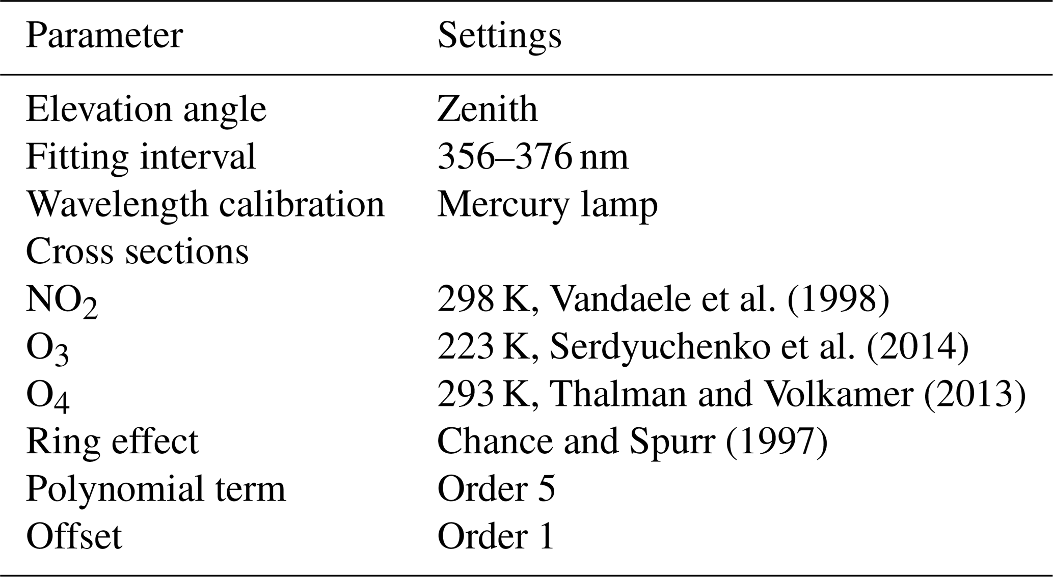
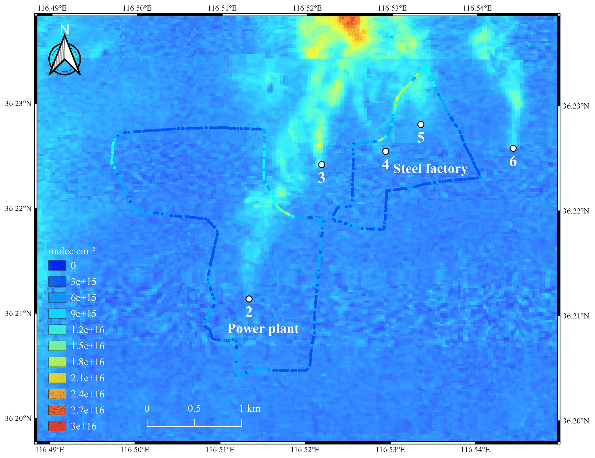
Figure 13 Overview of VCDs retrieved from the ground-based mobile DOAS system (circle marks) and VCDs retrieved by UVHIS (background layer) measured on 23 June 2018.

For better comparison with the UVHIS NO₂ observations, assumptions and parameters in the tropospheric NO₂ retrieval method for the mobile DOAS were similarly set to those of the UVHIS. For example, the residual amount of NO₂ in the reference spectra was set to 3×10¹⁵ molec cm⁻² with an error of 1×10¹⁵ molec cm⁻²; the mobile DOAS observations only focused on the tropospheric portion of the NO₂ columns, assuming that the difference in the stratospheric NO₂ columns between the observed and reference spectra is negligible; the vertical profiles of NO₂ and aerosol extinction, albedo and aerosol properties in the AMF calculation were similarly set to those of the UVHIS.

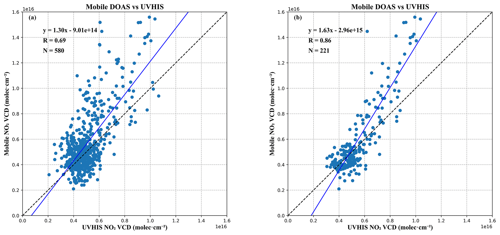
Figure 14 Scatter plot and linear regression analysis of the co-located NO₂ VCDs, retrieved from the UVHIS and mobile DOAS system, (a) for all co-located measurements, with a time offset of 1 h, (b) for co-located measurements that only circled the steel factory, with a time offset of 15 min.

Like the uncertainty analysis of the UVHIS NO₂ columns, the total uncertainty on the retrieved mobile tropospheric VCD is composed of three parts: (1) the mean uncertainty on the dSCD of the mobile DOAS is 1.4×10¹⁵ molec cm⁻²; (2) the uncertainty of reference vertical column is estimated to be 1×10¹⁵ molec cm⁻². In the case that the tropospheric AMFs of the measured and reference spectra are very close, this part results in an uncertainty of 1×10¹⁵ molec cm⁻² to the total uncertainty; (3) the mean relative uncertainty on the AMF calculation is 22 % by the square root of the quadratic sum of the individual uncertainties like UVHIS. Combining these uncertainties together, the mean total uncertainties on the retrieved tropospheric NO₂ VCD is 2.1×10¹⁵ molec cm⁻².

Basically, the route of the mobile DOAS was designed to encircle the power plant and the steel factory which are supposed to be predominant sources. For comparison, the mobile DOAS observations are first gridded to the same sampling of the UVHIS pixels. Then the VCD of the UVHIS NO₂ results is extracted for each co-located mobile measurement. An overview of the mobile DOAS measurements over the UVHIS NO₂ layer is shown in Fig. 13. The NO₂ distributions of the mobile DOAS system and the UVHIS exhibit similar spatial characteristics; i.e. low values are in the south of the steel factory and power plant, and high values are inside the plumes.

Figure 14a shows scatter plots with the VCDs retrieved by the UVHIS on the x axis and the mobile DOAS VCDs on the y axis for all co-located measurements. The corresponding results of the linear regression analysis are also provided in Fig. 14a, with a correlation coefficient of 0.69, a slope of 1.30 and an intercept of $-\mathrm{9.01}\times {\mathrm{10}}^{\mathrm{14}}$. The absolute time offset between the mobile DOAS and airborne observations can be up to 1 h, indicating that both instruments cannot sample the NO₂ column at certain geolocations simultaneously. As shown in Fig. 14b, when only comparing UVHIS VCDs to mobile measurements that circled the steel factory, the correlation coefficient improved to 0.86. In this case, all mobile measurements occurred inside the swath of one flight line of aircraft, and the time offset between two instruments is shortened to 15 min. In general, an underestimation of the UVHIS VCDs of increased value can be observed in Fig. 14a and b. Considering the variability in local emissions and meteorology, it is reasonable that the differences between these two instruments exist. A sensitivity test of the AMF on the NO₂ profile was performed for all co-located measurements, using a box profile of 500 m. Compared to the box profile of 2 km, the UVHIS AMFs decreased by an average of 17 %, whilst the mobile DOAS AMFs decreased by an average of 2.7 %. These results suggest that a more realistic profile with the NO₂ layer closer to the ground could improve the slope and bring it closer to unity.

7 Conclusions

In this paper, we present the newly developed UVHIS instrument, with a broad spectral region ranging from 200 to 500 nm and a high spectral resolution better than 0.5 nm. The instrument is operated in three channels at wavelengths of 200 to 276 nm (channel 1), 276 to 380 nm (channel 2) and 380 to 500 nm (channel 3) for minimal stray light effects and the highest spectral performance. The optical design of each channel consists of a fore-optics with a FOV of 40^∘, an Offner imaging spectrometer and a CCD array detector of 1032×1072 pixels.

We also present the first tropospheric NO₂ retrieval results from the UVHIS airborne observation in June 2018. The research flight over Feicheng, China, covered an area of approximately 30 km×20 km within 3 h, with a high spatial resolution approximately 25 m×22 m. We first retrieved the differential NO₂ slant column densities from nadir-observed spectra by applying the DOAS technique to a mean reference spectra over a clean area. Then we converted those NO₂ slant columns to tropospheric vertical columns using the air mass factors derived from the SCIATRAN model with the Landsat 8 surface reflectance product. The total uncertainties of the tropospheric NO₂ vertical columns range from 1.5×10¹⁵ to 5.9×10¹⁵ molec cm⁻², with a mean value of 3.0×10¹⁵ molec cm⁻².

The two-dimensional distribution map of the tropospheric NO₂ VCD demonstrates that the UVHIS is adequate for trace gas pollution monitoring over a large area in a relatively short time frame. With the high spatial resolution of the UVHIS, different local emission sources can be distinguished, fine-scale horizontal variability can be revealed, and trace gas emission and transmission can be understood. For the flight on 23 June 2018, the NO₂ distribution was dominated by several exhaust plumes which exhibited the same south-to-north direction of transmission, with a peak value of 3×10¹⁶ molec cm⁻² in the dominant plume. The comparisons of the UVHIS NO₂ vertical columns with the mobile DOAS observations show a good overall agreement, with a correlation coefficient of 0.65 for all the co-located measurements and a correlation coefficient of 0.86 for the co-located measurements that only circled the steel factory. However, an underestimation of the high NO₂ columns of the UVHIS is observed relative to the mobile DOAS measurements.

The high-resolution information about the NO₂ horizontal distribution generated from UVHIS airborne data is unique and valuable compared to those from ground-based instruments and space-borne sensors. In future studies, the UVHIS could be applied in the validation of satellite trace gas instruments and in the connection between local point observations, air quality models and global monitoring from space.