the Creative Commons Attribution 4.0 License.
the Creative Commons Attribution 4.0 License.
 | 18 Jun 2021
Identification of snowfall microphysical processes from Eulerian vertical gradients of polarimetric radar variables
Noémie Planat
Josué Gehring
Étienne Vignon
Polarimetric radar systems are commonly used to study the microphysics of precipitation. While they offer continuous measurements with a large spatial coverage, retrieving information about the microphysical processes that govern the evolution of snowfall from the polarimetric signal is challenging. The present study develops a new method, called process identification based on vertical gradient signs (PIVSs), to spatially identify the occurrence of the main microphysical processes (aggregation and riming, crystal growth by vapor deposition and sublimation) in snowfall from dual-polarization Doppler radar scans. We first derive an analytical framework to assess in which meteorological conditions the local vertical gradients of radar variables reliably inform about microphysical processes. In such conditions, we then identify regions dominated by (i) vapor deposition, (ii) aggregation and riming and (iii) snowflake sublimation and possibly snowflake breakup, based on the sign of the local vertical gradients of the reflectivity ZH and the differential reflectivity ZDR. The method is then applied to data from two frontal snowfall events, namely one in coastal Adélie Land, Antarctica, and one in the Taebaek Mountains in South Korea. The validity of the method is assessed by comparing its outcome with snowflake observations, using a multi-angle snowflake camera, and with the output of a hydrometeor classification, based on polarimetric radar signal. The application of the method further makes it possible to better characterize and understand how snowfall forms, grows and decays in two different geographical and meteorological contexts. In particular, we are able to automatically derive and discuss the altitude and thickness of the layers where each process prevails for both case studies. We infer some microphysical characteristics in terms of radar variables from statistical analysis of the method output (e.g., ZH and ZDR distribution for each process). We, finally, highlight the potential for extensive application to cold precipitation events in different meteorological contexts.
- Article
(12811 KB) - Full-text XML
-
Supplement
(1738 KB) - BibTeX
- EndNote


The characterization and modeling of snowfall necessitate a thorough understanding of the dynamical and microphysical processes driving snowflakes growth and evolution from the synoptic to the microscale (e.g., Ryzhkov and Zrnić, 2019; Morrison et al., 2020). Identifying and quantifying microphysical processes require the collection of accurate observations. Despite solid precipitation being generally frequent in polar climates and mountainous regions, ground-based or in situ measurements of clouds and precipitation remain limited in such areas due to the harsh meteorological conditions and sparsity of meteorological stations. Moreover, few methods and metrics exist to systematically and operationally give access to the occurrence and properties of microphysical processes in mountainous and polar snowfall.
Ground-based remote sensing instruments make it possible to gain insights into precipitation formation and vertical evolution in remote areas at high altitude and latitude (e.g., Shupe et al., 2011; Grazioli et al., 2015; Gorodetskaya et al., 2015; Wen et al., 2016; Grazioli et al., 2017a; Scarchilli et al., 2020; Lubin et al., 2020).
The added value of radar polarimetry (e.g., Kumjian, 2012; Tiira and Moisseev, 2020) is of particular relevance for characterizing salient features in radar profiles, like the melting layer (Griffin et al., 2020), but also for deciphering the microphysical structure of snowfall. Bader et al. (1987), Andrić et al. (2013), Schneebeli et al. (2013), Moisseev et al. (2015), Grazioli et al. (2015), Besic et al. (2018) and Gehring et al. (2020), among others, show the potential of dual-polarization variables for studying some characteristics of snowflakes (e.g., type, shape, orientation, size and phase) and the underlying microphysical processes that drive their evolution.
However, the complex microphysical properties of snowflakes (i.e., large variety in density, size and shape) hamper an accurate and universal retrieval of their physical and geometrical properties from polarimetric radar data. Various studies used different polarimetric and Doppler signatures to identify the main cold processes (aggregation, vapor deposition, sublimation and riming), depending on the context. For instance, the onset of aggregation was identified by Moisseev et al. (2015) as bands of high values of specific differential phase Kdp. Kennedy and Rutledge (2011) and Gehring et al. (2020) identified a region dominated by aggregation with a decrease in differential reflectivity (ZDR) collocated with an increase in reflectivity (ZH), while Schrom and Kumjian (2016) identified aggregation as a maximum in the downward relative gradient of reflectivity ∂zZH below the −15 ∘C isotherm and a positive downward gradient of absolute Doppler velocity .
Various methods have also been developed to extract information from the spatial and temporal evolution of radar polarimetric variables. The quasi-vertical profiles (QVPs) method was introduced by Ryzhkov et al. (2016). QVPs are computed from plan position indicator (PPI) radar scans at different elevation angles that are azimuthally averaged to give vertical profiles of polarimetric variables above the radar. A similar method named columnar vertical profiles (CVPs) provides vertical profiles at any point in space and was presented in Murphy et al. (2020). The authors emphasize that the noise and standard deviation of the signal are strongly reduced owing to the azimuthal averaging. Range height indicator (RHI) scans can also be used to extract vertical profiles at a given azimuth (e.g., Andrić et al., 2013; Moisseev et al., 2015; Gehring et al., 2020). The analysis of vertical profiles of dual-polarization variables from RHI scans has been further developed by Tiira and Moisseev (2020) with a multivariate unsupervised classification of vertical profiles of ZH, ZDR and Kdp. The mean profiles of the resulting classes have been a posteriori interpreted in terms of specific meteorological conditions and microphysical processes.
One should, however, be careful when interpreting the vertical profiles obtained with those methods in conditions of strong wind shear. Indeed, strong wind shear leads to slanted streamlines of snowflakes, thereby manifesting as clear fall streaks in RHI scans or time–height plots. In such cases, the shape of the vertical profiles of radar variables strongly depends upon advection mechanisms and not only on microphysics. Kalesse et al. (2016) discuss this issue by characterizing the hydrometeor properties through the analysis of gradients of radar variables along the pre-identified fall streaks during a snowfall event in Finland. However, in which conditions one can reliably associate the local vertical profiles of polarimetric variables to the occurrence or intensity of a given microphysical processes in snowfall is still, to our knowledge, an open question.
In the present study, we propose a new method to automatically identify the microphysical processes in snowfall from dual-polarization radar quantities. This method, referred hereafter to as PIVSs (process identification based on vertical gradient signs), is systematic and based on vertical gradients of ZH and ZDR, therefore focusing on the vertical evolution of the particles characteristics. PIVSs will help characterize the occurrence and properties of the dominant microphysical processes governing the snowfall evolution in space and time. A preliminary step consists of developing an analytical framework to theoretically determine the conditions in which the vertical (Eulerian) analysis of polarimetric radar signal provides robust information about snowfall microphysics. This method is then illustrated over two case studies to identify and characterize the microphysical processes at play, i.e., one case at Dumont d'Urville (DDU) station, Adélie Land, Antarctica, and one case in the Taebaek Mountains, South Korea. As the two events correspond to different hemispheres and different meteorological and orographic conditions, their analysis will help illustrate the range of applications of the designed method.
The paper is structured as follows. We first derive and discuss the analytical framework in Sect. 2. We then present the development of our method and its implementation in Sect. 3. Section 4 illustrates the method application over the two case studies and discusses the outcome and the associated limitations. We then summarize our key findings and draw the conclusions in Sect. 5.
The vertical structure of radar polarimetric variables strongly depends on how microphysical processes modify the properties of the crystals and snowflakes. As mentioned above, different studies have exploited the vertical profiles of polarimetric radar variables to identify and characterize microphysical processes. One may, nonetheless, question the approach when additional mechanisms alter the evolution of radar variables along the vertical direction. This is, for example, the case when strong generating cells are present at the top of the cloud and the associated precipitating particles sediment. When advected, the horizontally heterogeneous snowfall manifests as so-called fall streaks which induce vertical gradients of polarimetric variables. Analyses of microphysical processes along fall streaks (i.e., following the snow particles in a Lagrangian framework) are very relevant and give insights into the microphysical evolution of complex precipitation systems (e.g., Pfitzenmaier et al., 2018). However, fall streak retrieval algorithms are based on the accurate acquisition of the 3D wind field, which is often not available from measurements. Since the proposed method of the snowfall microphysical process characterization will be based on the interpretation of local vertical gradient in Eulerian vertical profiles of polarimetric radar variables (see Sect. 3), it is, hence, crucial to clearly define the meteorological conditions in which such gradients give access to reliable information about microphysical processes and, therefore, the conditions in which our method can be applied. These conditions will be dictated by both the 3D wind field (to avoid, e.g., strong updrafts or significant wind shear favorable for fall streaks) and the spatial heterogeneity of the radar fields ZH and ZDR.
Let us first consider the continuity equation for radar reflectivity ZH (Passarelli, 1978; Milbrandt and Yau, 2005). A similar continuity equation can be developed for other extensive radar variables, such as ZDR, and, therefore, similar developments hold, i.e., similar conditions on the characteristic scales of variation can be derived as follows:
where z denotes the vertical coordinate oriented upward, vz is the reflectivity-weighted sedimentation velocity vector, and u is the wind vector whose respective components in the (x, y and z) directions are (u, v and w). represents all the microphysical source/loss terms for ZH, while the rightmost term of the equation is the particle sedimentation term.
Once developed, this equation reads as follows:
With no loss of generality, one can work in a 2D framework along the horizontal wind direction (denoted x for convenience here). Equation (2), hence, reads as follows:
One can notice that the reflectivity source/loss terms can be directly related to the vertical gradient of reflectivity – multiplied by the relative vertical velocity of the flow with respect to hydrometeors – if the other terms in the equation are negligible.
In what follows, we, thus, assess in which conditions the equality,
is verified. Let us note (respectively, and ) the characteristic value of the horizontal wind velocity u (respectively, of ZH and of relative vertical velocity w−vz). Ld, X refers to the scale of variation in the variable X in the direction d. To verify Eq. (4), it is sufficient to satisfy the following three conditions:
Condition 1. The horizontal divergence term is negligible with respect to the vertical divergence and sedimentation, i.e., the velocity field is sufficiently homogeneous horizontally and the horizontal advection of ZH horizontal inhomogeneities is negligible. This condition mathematically reads:
which, after approximating a derivative by the ratio of typical scales and removing , turns into the following:
In stratiform snowfall conditions, the horizontal wind speed (respectively, the relative fall speed velocity) is frequently smoother than the radar reflectivity in the horizontal (respectively, vertical) direction. In such situations, Eq. (7) approximates to the following:
and condition 1, thus, reduces to ensure that the horizontal advection timescale of the reflectivity is much smaller than the vertical one.
Condition 2. The vertical divergence of (w−vz)ZH is mainly driven by the variations in ZH itself and not by variations in the relative vertical velocity. In other words, the vertical changes in the relative vertical velocity are small compared to the vertical changes in reflectivity, that is:
or in terms of typical scales:
Condition 3. The system is quasi-stationary. In other words, when this condition is verified, the timescales of variations due to microphysical processes are comparable with the typical timescale associated with particle sedimentation in such a way that the vertical profile of reflectivity always remains close to the equilibrium solution, as follows:
or in terms of variable dimension:
When respected, Eqs. (7), (9) and (11) thus express sufficient physical conditions in which the local vertical gradient of ZH (times the relative vertical velocity) is thereby directly related to the dominant microphysical processes and can be used to identify the occurrence and the properties thereof. The same approach can be used for the vertical gradient of ZDR.
We can now introduce the so-called PIVS method to identify the occurrence of microphysical processes in snowfall from the vertical gradients of polarimetric radar variables. The different steps of the method are successively described hereafter and are schematically represented in Fig. 1. It is worth noting that our method is built on ZH and ZDR vertical gradients only because these two polarimetric variables show strong signatures in the two events studied in Sect. 4 – as opposed to Kdp for which no pattern was observed in the Antarctic event EV1 – and because we aim to keep the method simple and robust at first. These two variables will make it possible to perform a process classification into three main groups, and we discuss, in Sect. 3.2, a possible method extension using additional polarimetric variables. Moreover, note that ZH and ZDR gradients are not affected by possible miscalibrations.
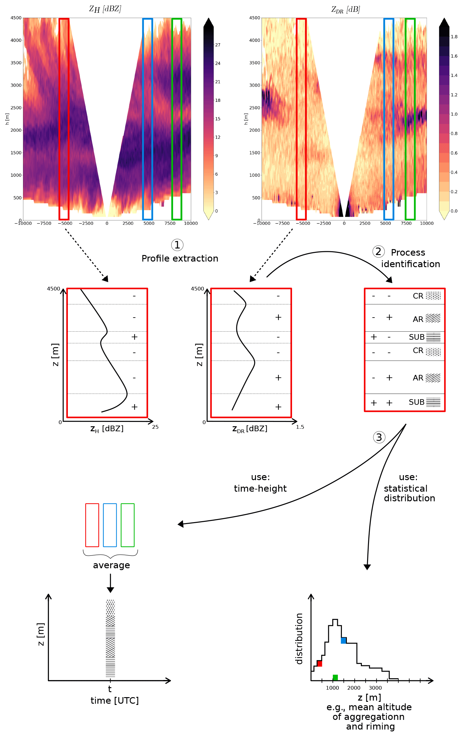
Figure 1Schematic of the PIVS method. The two top panels are examples of RHI scans of ZH and ZDR.
With the method being based on the vertical gradients of ZH and ZDR, it can be reliably applied to snowfall events that respect the three conditions (Eqs. 7, 9 and 11) for both ZH and ZDR. The method then consists of three main steps. We first present how to extract the vertical profiles of radar variables from RHI scans, and then we explain how to identify processes from the analysis of vertical gradients of ZH and ZDR. We finally develop the statistical framework to analyze and interpret the results of the method.
3.1 Step 1: vertical profiles extraction in RHI scans
The first step aims to extract vertical profiles of ZH and ZDR from 2-dimensional RHIs. We want the resulting profiles to correctly capture the vertical evolution of the snowfall and contain the microphysical information without being too sensitive to the parameters involved in the extraction procedure.
3.1.1 Selection of non-empty RHIs
We first select the RHIs with enough signal to be robustly used as input for the PIVS algorithm. We keep the RHIs in which the percentage of occupied gates in an area covering Dx kilometers in the horizontal range and Dz kilometers in the vertical range exceeds a minimum threshold of p%. The Dx×Dz area is chosen considering the sensitivity of the radar (Dx should delimit the area where the sensitivity is high enough), the vertical extent of the precipitating clouds (limiting Dz), the potential presence of a melting layer (potential lower vertical limit, since the method is not applicable in and below the melting layer; see below), and the orography. In conditions where the orography or the nature of the surface is very different between the left and the right part of the RHI, one should consider treating the two different RHI sides independently.
3.1.2 Time averaging of the RHIs
Once RHIs have been properly selected, we apply a time averaging to smooth part of the noise out. Microphysical processes have typical timescales ranging from a few minutes to a few hours. In order to remove noise and keep the microphysical signal, the chosen averaging time (hereafter Δt) should thus be lower than a few tens of minutes. Because our radar provides RHIs approximately every 5 min (see Sect. 4.1), averaging two consecutive RHIs is a reasonable trade-off.
3.1.3 Horizontal division of the RHIs and vertical profile extraction
One can now extract the vertical profiles from the RHIs. RHIs are initially acquired in an elevation × range grid that we project onto a 75×75 m2 resolution Cartesian grid (note that 75 m is the range resolution of our radar; see Sect. 4.1), then we select columns of signal. To further reduce the noise, we also apply a horizontal spatial averaging and extract the median column among neighboring columns. This step is delicate since the spatial variability of the microphysical processes has to be conserved. The horizontal average distance is noted Δx and is typically chosen between 5 % to 10 % of Dx. Profiles are then extracted every .
3.1.4 Selection of usable profile sections and vertical smoothing
We then select the relevant sections of the vertical profiles and perform final processing procedures to obtain a consistent data set.
-
In the top part of the extracted profiles, there might be only a few gates containing significant signal (signal-to-noise ratio above 0 dB). We calculate and keep the median vertical profile at a certain height only if at least 70 % of the gates contain significant signal.
-
One- and two-gate signal gaps, mostly located at the top of the profiles, are replaced with linearly interpolated values from the two nearest gates. Then we only keep the parts of the profiles that contain more than six gates with significant signal.
-
Finally, we apply a vertical three-gate window moving average to reduce gate-to-gate noise.
3.2 Step 2: process identification
Once profiles have been extracted from RHI scans, we compute along each of them the local gradients of reflectivity ZH and differential reflectivity ZDR at each altitude. Based on Eq. (4), we use the sign of the those gradients to identify the dominant process – i.e., the process that predominantly drives the local evolution of reflectivity or differential reflectivity – at a given altitude.
Based on past literature, we set criteria to assign a given ZH and ZDR local vertical gradient sign configuration to a given microphysical process. It is worth noting that the following criteria only hold in snowfall and are not valid for processes within or below the melting layer. Importantly, such criteria are valid only in situations in which hydrometeors have a negative absolute vertical velocity. In strong updrafts, i.e., in case of positive net vertical velocity, a given microphysical process will manifest in the radar profile with an opposite vertical gradient sign (see Eq. 4). It is worth emphasizing that the PIVS method is based only on the sign of the gradients, regardless of their magnitude. As in Sect. 2, we adopt the convention that the vertical axis is oriented upward.
-
Aggregation and riming (hereafter AR) correspond to an increase in reflectivity due to an increase in particle size and/or density with decreasing altitude () and a decrease with decreasing height in ZDR (). This decrease in ZDR is due to the decrease in particle density (larger snowflakes being less dense) and to the more chaotic orientation of the snowflakes associated with their increase in size and Reynolds number (Li et al., 2018; Ryzhkov and Zrnić, 2019). Riming is a complicated process regarding ZDR, mostly due to the opposite effects of decreasing oblateness (hence, a decrease in ZDR) and increasing density (hence, an increase in ZDR). The dominant effect was reported to be an overall decrease in ZDR (Ryzhkov and Zrnić, 2019). ZDR, thus, behaves slightly differently for aggregation and riming, but to our knowledge, it is complicated to differentiate them only from the sign of the vertical gradients of ZH and ZDR. We, therefore, decided to group these two processes together.
-
Crystal growth by vapor deposition (hereafter CG) corresponds to an increase in particle size with decreasing height () and an increase in oblateness with decreasing height () as particles generally grow along their longest dimension (Schneebeli et al., 2013; Andrić et al., 2013; Grazioli et al., 2015). The decrease in density during CG acts the opposite way to the increase in oblateness on ZDR (through the dielectric constant). However, since in ZDR the oblateness is weighted in D6, the contribution from the increase in oblateness generally dominates over the decrease in density and, overall, contributes to an increase in ZDR during CG.
-
Sublimation (hereafter SUB) corresponds to a downward relative decrease in particle size and concentration (, Grazioli et al., 2017b). Because we define SUB only based on ∂zZH, it may potentially include other processes that diminish the radar reflectivity (notably the breakup of snowflakes; see Ryzhkov and Zrnić, 2019).
Aggregation, riming, crystal growth and sublimation do not form an exhaustive list of snowfall microphysical processes. Future improvements of the method may consider the variations in ZDR also in the SUB category and/or evolution of Kdp and cross-correlation coefficient ρhv. This could help distinguish riming/aggregation and identify more processes, notably secondary ice generation processes (very active in Antarctica; see Sotiropoulou et al., 2021) that can be associated with strong signatures in Kdp (Sinclair et al., 2016).
3.3 Step 3: data analysis and visualization
To visualize and analyze the 3-dimensional (height, horizontal distance to radar and time) output of the method, and apart from inspecting each RHI individually, we employ time–height plots and statistical distributions to synthesize the information. Time–height plots are built as follows. For each altitude range and each time step, we compute the proportion of each microphysical process among the extracted vertical profiles in the horizontal direction within the corresponding RHI scan. We, hence, estimate the dominant process at a given time and at a given height as the process showing the largest occurrence in the horizontal direction within the RHI. Regarding statistical distributions, we compute the empirical distributions of different variables (e.g., occurrence height and magnitude of the vertical gradient) conditioned or not to a specific process. The large number of profiles in the considered case studies (see Sect. 4) ensures the robustness of the derived statistics.
We now present two case studies of snowfall events, namely one over the coast of the Antarctic continent (hereafter EV1) and one over South Korea (hereafter EV2). The two considered precipitation events are produced by stratiform clouds associated with the passage of a warm front above the location of interest. The meteorological and geographical conditions are, however, quite different, particularly in terms of the synoptic moisture advection and effects of the orography and of low-level flows on precipitation. Hence, we can test, appreciate and discuss our method during two contrasted snowfall events.
4.1 Campaigns and data sets
4.1.1 APRES3 (Antarctic Precipitation, Remote Sensing from Surface and Space) campaign in coastal Adélie Land, Antarctica (EV1)
The first precipitation event was sampled in the framework of the Antarctic Precipitation, Remote Sensing from Surface and Space (APRES3) campaign that took place at the French Antarctic station of Dumont d'Urville (DDU), coastal Adélie Land, Antarctica. DDU station is set up on Petrel Island (−66.66∘ S, 140.00∘ E; 41 m a.s.l.; UTC+10), 5 km off the landfall of the ice sheet.
A noticeable weather feature at DDU is the low-level katabatic flow blowing down from the high Antarctic Plateau with an easterly to southeasterly direction. This strong and dry flow, vertically extending up to ≈1.5 km, significantly diminishes the amount of precipitation that reaches the ground by sublimating the snowflakes (Grazioli et al., 2017b; Durán-Alarcón et al., 2019; Vignon et al., 2019b).
The APRES3 campaign was heavily instrumented during austral summer 2015–2016 (Grazioli et al., 2017a; Genthon et al., 2018). Of particular relevance for our work is that an X-band dual-polarization Doppler radar (mobile X-band polarimetric weather radar – MXPOL; Schneebeli et al., 2013; Scipión et al., 2013) was deployed. It scanned the atmosphere with a range resolution of 75 m, a maximal range of 30 km and a Nyquist velocity of 39.8 m s−1. The scan strategy for EV1 was a repeating succession of two PPI at low elevations, one vertical profile and two RHI scans approximately parallel and perpendicular to the prevailing katabatic wind direction. This total scan strategy took about 5 min. In the data processing, we have only kept the parts of the RHIs for which the elevation angle is greater than 5∘ – to avoid ground clutter – and lower than 45∘ – to conserve reliable polarimetric signal – and for which the altitude with respect to the radar is greater than 500 m to avoid near-field effects. The results presented in this study are from the 203∘ RHI scans, which are more parallel to the direction of the large-scale moisture advection.
The semi-supervised hydrometeor classification algorithm of Besic et al. (2016) has also been applied on the MXPOL RHI scans to determine the hydrometeors' nature from the polarimetric signal. Using the additional demixing module from Besic et al. (2018) makes it possible to further infer the proportions of different hydrometeor types within a given radar sampling volume.
In addition to MXPOL, a multi-angle snowflake camera (MASC; Garrett et al., 2012) was deployed. Hereinafter, we use the products of the hydrometeor classification from MASC images developed by Praz et al. (2017). A preliminary processing step, following Schaer et al. (2020), removes blowing snow particles from the data set. A pluviometer was also continuously measuring the precipitation rate during the event (Grazioli et al., 2017a; Genthon et al., 2018).
The precipitation event of interest took place between 28 and 30 December 2015. It was associated with the passage of a warm front of an extra-tropical cyclone setting at the west of DDU. This type of precipitation system is typical for DDU (Jullien et al., 2020). The accumulated precipitation at the ground during the event was 3.4 mm (Vignon et al., 2019a).
4.1.2 ICE-POP campaign in South Korea (EV2)
The second case study took place on 28 February 2018 in the Taebaek MOUNTAINS, near Pyeongchang, in South Korea. It was an intense precipitation event (55 mm of equivalent liquid precipitation) associated with a warm conveyor belt (WCB; i.e., a warm and moist airstream ascending along the cold front of an extratropical cyclone; see Green et al., 1966; Harrold, 1973; Browning et al., 1973). The event was sampled by the suite of instruments deployed during the International Collaborative Experiments for Pyeongchang 2018 Olympic and Paralympic winter games (ICE-POP 2018) and thoroughly studied in Gehring et al. (2020).
A total of two main sites at different altitudes and locations were instrumented (see Fig. 1 in Gehring et al., 2020). The lowest site (66 m a.s.l.) was the Gangneung-Wonju National University (GWU) close to the shore. The second, Mayhills site (MHS), was located more inland in the Taebaek massif at 789 m a.s.l.
The same MXPOL radar as that used during the Antarctic APRES3 campaign was deployed at GWU with a scan strategy adapted to the orography and the location of the two Korean measurement sites. RHIs scans with a range resolution of 75 m and an horizontal range of 27.2 km were performed towards MHS at two slightly different azimuths (225 and 235∘). The total scan strategy lasted 10 min, with repetition in the main RHI directions every 5 min. As for the APRES3 campaign, we processed the RHIs in a way to keep only the part for which elevation angles are ≥5 and ≤45∘. Moreover, due to important ground echoes, we will analyze the signal only above an altitude of 2000 m a.g.l. (above ground level). At the MHS site, the MASC collected images of falling snowflakes, while a 94 GHz W-band Doppler cloud profiler (WProf; Küchler et al., 2017) provided high-resolution measurements of the reflectivity and of the full Doppler spectra, with a Nyquist velocity of 5.1 m s−1 (dealiased; see Gehring et al., 2021 for details). A pluviometer also measured the precipitation rate during the entire event.
4.2 Applicability of the method and implementation
Before applying the method to the case studies, we must verify that the environmental conditions derived in Sect. 2 are fulfilled so that the local vertical gradients are mostly governed by – and subsequently reflect – microphysics. More precisely, Eqs. (7), (9) and (11) should be satisfied. For this purpose, we need to estimate the characteristic scales , , , Lx,u, , , , and Lz,w during the two events.
is obtained by calculating the mean wind velocity from radiosoundings between 500 m (EV1) or 2000 m (EV2) and Dz a.g.l. during the events (see Vignon et al., 2019a, b; Gehring et al., 2020 for details on radiosonde data acquisition and processing). is measured from vertical Doppler velocity measurements. We use MXPOL data for EV1, while we prefer using WProf measurements for EV2 given its higher temporal frequency. Note that the vertical Doppler velocity gives direct access to the net (particles size distribution weighted) sedimentation velocity (w−vz).
Following Skøien et al. (2003), we then determine the characteristic space scales and timescales by means of variogram estimated from radar RHI scans. The variograms are normalized by the variance in the field along the direction we use to compute the variogram (see Lebel and Bastin, 1985). Skøien et al. (2003) quantify the characteristic length (or time-) scales in non-stationary fields by visually localizing the first significant slope change – indicating the shortest decorrelation scale – in variograms plotted with logarithmic axes. As the wind and radar 4D fields are generally non-stationary (in a statistical sense), we follow the same approach except that, in our case, the spatial extent of ZH and ZDR is not sufficient to properly work with logarithmic axes.
Note, however, that the horizontal variations of the wind, ZH and ZDR can occur over typical distances that exceed the visibility range of the radar (10 to 15 km for EV1; 15 to 20 km for EV2). This prevents a robust estimation of the horizontal decorrelation distances. Therefore, we estimate the horizontal characteristic length scales from numerical simulations carried out with the Weather Research and Forecasting model (WRF; see Appendix A). As the X-band radar reflectivity and differential reflectivity are not standard variables of WRF, we calculate the variogram of the sixth moment of the snow particle size distribution (which the radar is the most sensitive to). In fact, under simplifying assumptions (namely constant density and spherical shape), the radar reflectivity in the Rayleigh regime is proportional to the sixth moment of the particle size distribution of snow particles.
Because the original data set is 3-D (4-D for the WRF data set), we extract variograms (along any direction) that are also 3-D (4-D). Therefore, the mean and percentiles displayed (and the calculation of the decorrelation length) are computed based on the averaged signal along one (or two) dimension(s) (unless specified, we prefer to temporally average the signal). The variograms are plotted in Fig. S1 for EV1 and in Fig. S2 for EV2 in the Supplement. The obtained values for , , , Lx,U, Lx,Z, Lz,Z, , and Lz,w are summarized in Table 1.
Table 1Summary of the characteristic scales for the two events (see Figs. S1 and S2 for details). Ld,X refers to the scale of variation in the variable X in the direction d, and is the sixth moment of the snow particle size distribution from the WRF simulation, a proxy for ZH.
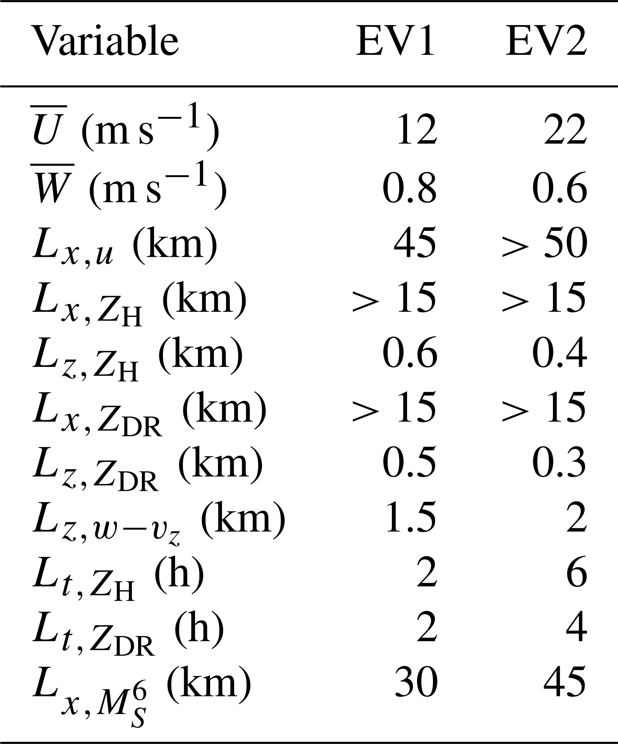
Table 2 shows that the three environmental conditions derived in Sect. 2 are verified for the bulk of the two case studies for ZH and ZDR and, therefore, legitimizes the use of vertical gradients and the applicability of PIVSs. To evaluate an upper limit for condition 1, we use km because we know km from the horizontal variogram of ZDR (not shown), but we cannot derive an accurate larger value from WRF simulations (the model hypothesizes spherical particles). We note that the third condition (stationarity) is largely respected, while the first and second conditions are less clearly respected. Particular attention should thus be paid to this aspect when analyzing the results in the next section, particularly when focusing on very local (in space and in time) patterns.
Table 2Verification of the three analytical conditions derived in Sect. 2 for the two case studies. Conditions 1, 2 and 3 correspond to Eqs. (7), (9) and (11) evaluated with ZH, while conditions 1', 2' and 3' are evaluated with ZDR.
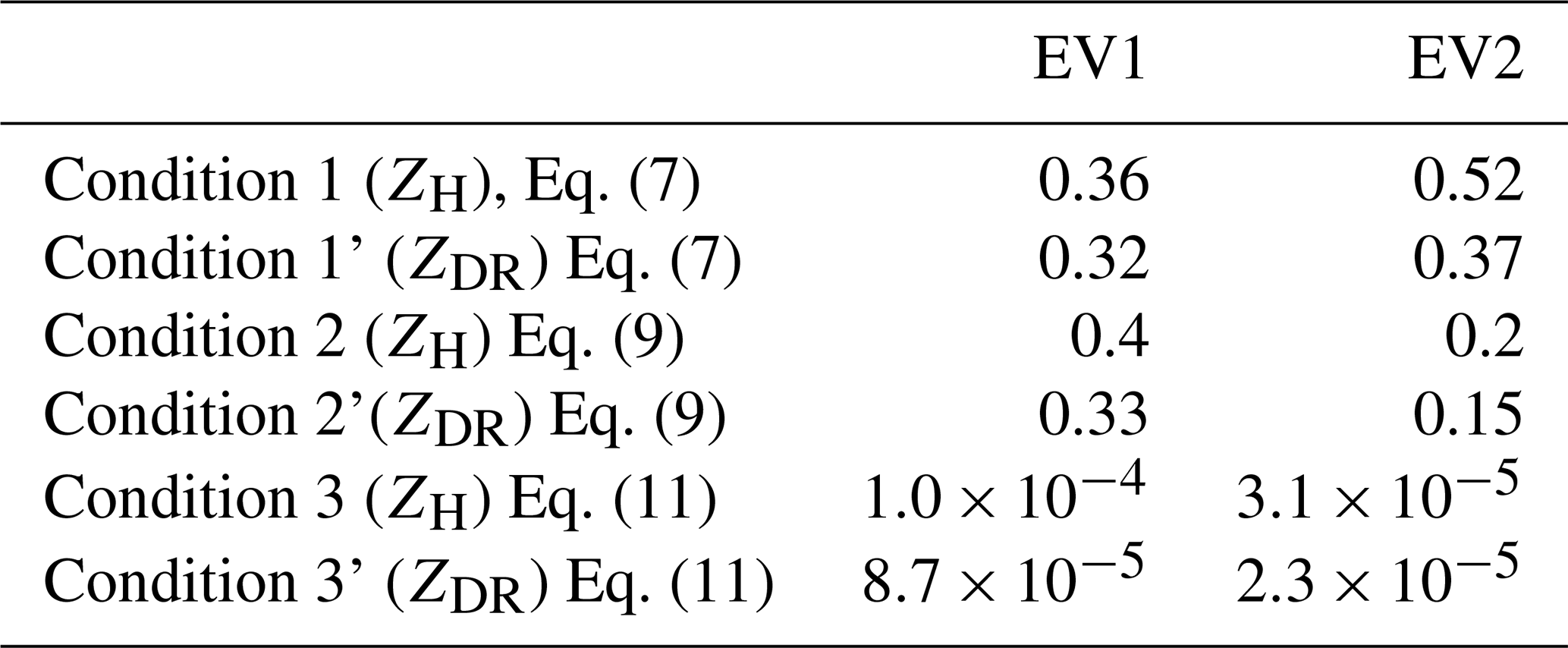
Table S1 in the Supplement further presents the processing parameters required for the implementation and selection following the guidelines of Sect. 3. The sensitivity to their exact values has been assessed (not shown), and we can underline that our results are not significantly sensitive to a change in these parameters by ±50 %.
4.3 Illustration of the method
Figure 2 illustrates the process identification patterns in a RHI scan during EV1. Overall, one can notice that the method reveals a quite characteristic (and expected) vertical pattern in terms of process occurrence: CG takes place mainly higher than AR (in this RHI, CG is around 3100–4200 m, and AR is between 3100 and 2000 m), which is itself higher than SUB (from 2000 to 500 m). This pattern is consistent with the typical structure of precipitation at DDU as already described in Grazioli et al. (2017a), Durán-Alarcón et al. (2019) and Vignon et al. (2019a). Cloud ice crystals first grow by vapor deposition, then start to sediment, aggregate and eventually rime when supercooled liquid water is present in the clouds. As dry katabatic winds keep blowing near the ground surface during the event, an approximately 1.5 km deep layer, exhibiting a decrease in reflectivity with decreasing height, is noticeable and reflects the enhanced sublimation of snowflakes.
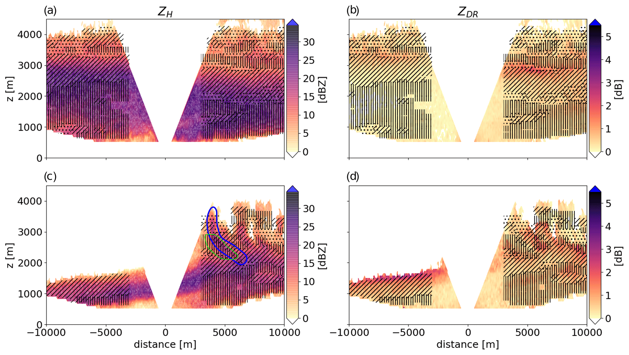
Figure 2Illustration of the PIVS method application on ZH (a) and ZDR (b) RHI scans during EV1 on 28 December 2015 at 21:48 UTC. (c, d) Illustration of fall streaks on 28 December 2015 at 10:20 UTC. (c) Blue lines highlight fall streaks, and green contours indicate regions where the PIVS method is probably not reliable. In all panels, the process identification of the PIVS method is superimposed with black symbols, i.e., dots locate the CG process, the AR process and the SUB process.
One should further remember that the conditions for applying the method derived from the theoretical framework in Sect. 2 were verified for the bulk of the event. Subsequently, such conditions may be not respected locally (in time and space). It is particularly the case for RHIs exhibiting fall streaks in conditions with strong wind shear, as in Fig. 2c–d (identified in blue in Fig. 2c) or ice pockets. Indeed, the reflectivity may increase along the fall streak, while a vertical analysis of the gradient rather reveals a decrease (and, therefore, SUB) of ZH with decreasing height (see the green area in Fig. 2c).
The temporal structure of the process identification by PIVSs is presented in Fig. 3 for EV1 and in Fig. 4 for EV2. Time–height plots of ZH and ZDR for the two events are plotted in Figs. S3 and S4, together with the type of the dominant process identified with PIVSs. Interestingly, the stratification of layers that we illustrated for a particular RHI in Fig. 2a–b is clearly visible during most of EV1 in Fig. 3. SUB and AR both clearly manifest as well defined layers, while CG is the dominant process at the top of the precipitating cloud. Albeit surprising, the thin upper layer of SUB visible around 3000 m between 28 December at 14:00 UTC and 29 December at 09:00 UTC concurs with a sub-saturated layer with respect to ice visible in the radiosoundings (see Fig. 3i). The occurrence of sublimation in this layer is thus very likely.

Figure 3Time–height plot of ZH (a) and of the process identification from the PIVS method during EV1 with (b) CR, (c) AR, (d) SUB and (e) the three categories. In panels (b–e), the gray shading indicates regions where dBZ. The dashed black lines in panel (a) show the temperature isotherms from the corresponding WRF simulation (extracted and averaged along the same RHI scan). The color bar in panels (b–d) refers to the percentage of gates at a given height within the RHI corresponding to a certain process. In panel (e), the color labeling indicates the dominant microphysical process. On the y axis, z is the altitude above ground level. Panel (f) presents the time series of the cumulative number of hydrometeors – classified into different categories, following Praz et al. (2017) and detected by the MASC. SP, CC, PC, AG, GR and CPC refer to small particles, columnar crystals, planar crystals, aggregates, graupel and combination of planar and columnar crystals, respectively. The black dashed line shows the precipitation measured at the surface with a snow gauge. Panels (g–j) show the radiosounding measurements, which are, respectively, temperature, wind direction, relative humidity with respect to ice (RHi) and wind speed. The colors of the profiles refer to different times indicated with thick vertical lines in panel (a). The red boxes delimit time periods during which aggregation is detected down to the ground by PIVSs and aggregates, and graupel are detected in a relatively high proportion (half of particles) by the MASC. The blue box indicates a period with at simultaneous intense reflectivity in the column and intense near-surface sublimation associated with few particles at the ground level. The orange box, a few hours later, shows when SUB weakens and when more particles are detected by the MASC.
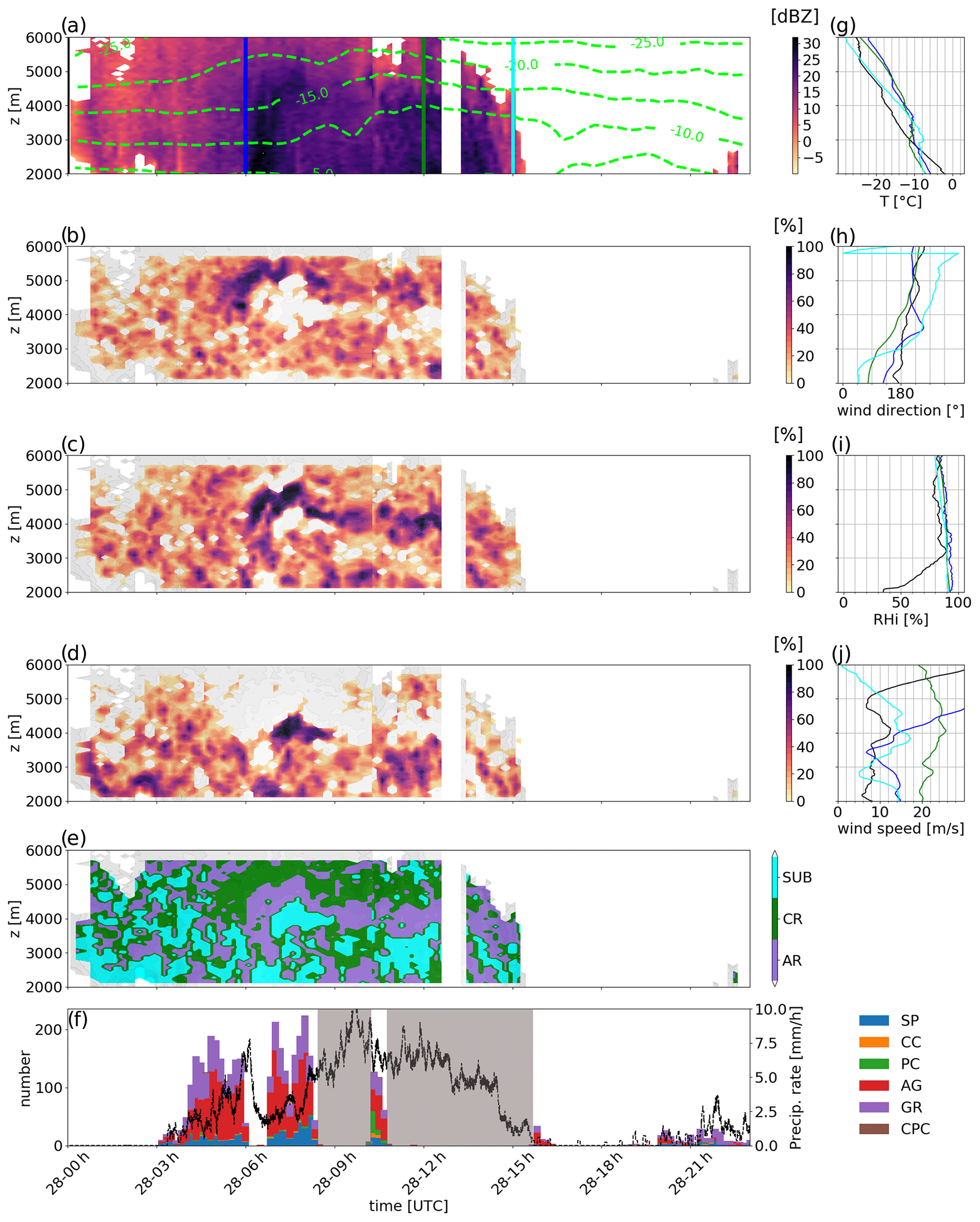
Figure 4Same as Fig. 3 for EV2 without the colored boxes. The gray areas in (f) mask periods during which the MASC was not working.
Regarding EV2, one can first notice that SUB occurs in the bottom part of the cloud before 04:00 UTC. This corresponds to virga clouds ahead of the warm front, which we can also identify in radiosoundings with a very dry layer visible at 00:00 UTC (see Fig. 4i). This is consistent with the conceptual model for precipitation evolution during the passage of the warm front of Gehring et al. (2020) and previous studies (e.g., Clough and Franks, 1991). Moreover, the PIVS method identifies crystal growth as the dominant process in the top layer of the cloud (≈ 4500–6000 m) and a layer of aggregation/riming below (≈ 4500–3500 m) during most of the event (from 06:00 to 12:00 UTC). These two layers persist during 6 h and are ≈ 500–1000 m deep during the core of the event.
Interestingly, the process identification with PIVSs provides a more broken-up pattern during EV2 than during EV1. This concurs with the fast-evolving synoptic system associated with the intense warm conveyor belt dynamics over Korea (Gehring et al., 2020). Notably, a well-marked region dominated by sublimation around 08:00 UTC at ≈4000 m can be pointed out. However, the radiosounding at 00:06 UTC reveals supersaturation with respect to ice in the corresponding layer (see Fig. 4i), making snowflake sublimation impossible. This particular inconsistency can be explained by an isolated – but strong – turbulent updraft (see more details in Appendix B). As specified in Sect. 3, the PIVS method only holds in conditions with a negative (towards the ground) net velocity of the hydrometeors, and it provides non-realistic results for very localized – in time and space – profiles with updrafts strong enough to move hydrometeors upward.
4.4 Comparison with MASC data and radar-based hydrometeor classification
We now compare the results of the PIVS method with surface MASC observations of ice crystals and snowflakes to assess its robustness. Figures 3f and 4f show a time series of the number of hydrometeors of different categories detected by the MASC during EV1 and EV2, respectively.
During EV1, most hydrometeors are small particles, owing to the intense sublimation by katabatic winds (and possible blowing snow not fully filtered out by the MASC processing; see Sect. 4.1). Between 00:00 and 05:00 UTC and between 17:00 and 19:00 UTC on 30 December 2015, the MASC detected a significant number of aggregates and graupel particles. During those periods, the PIVS method identifies aggregation/riming as being dominant at low levels, together with limited sublimation near the ground (Fig. 3b–e; red boxes). Moreover, the highest reflectivities measured in the column during these events are around 00:00 UTC on 29 December, while the MASC detects very few particles. This is consistent with the concomitant enhanced sublimation identified by PIVSs (Fig. 3d, blue box). A few hours later (around 06:00 UTC; orange box), SUB becomes slightly less active, and a larger number of particles is detected by the MASC.
During EV2, the MASC did not detect particles before 04:00 UTC on 28 February (see Fig. 4f), which is consistent with the sublimation layer identified between 2000 and 3000 m a.g.l. by PIVSs (Fig. 4d). Particles start being detected by the MASC around 04:00 UTC, which corresponds to the decay of the low-level sublimation layer. The majority of the particles identified by the MASC are aggregates and graupel between 04:00 and 08:00 UTC. However, Gehring et al. (2020) report a significant difference in terms of particle size distribution (PSD) over the time period. This explains why the PIVS signal for AR is relatively weak between 04:00 and 06:00 UTC; the aggregation is active, but aggregates are small, and their polarimetric radar signature is weak. Around 08:00 UTC 28 February 2018, the number of aggregates detected by the MASC reaches its maximum value, and Gehring et al. (2020) point out an increase in the mean size of observed aggregates. This peak is collocated with a well-defined layer of AR identified by PIVSs above.
We, therefore, obtain a fair consistency between the type and number of particles identified by the MASC at the surface and the microphysical processes identified by PIVSs aloft.
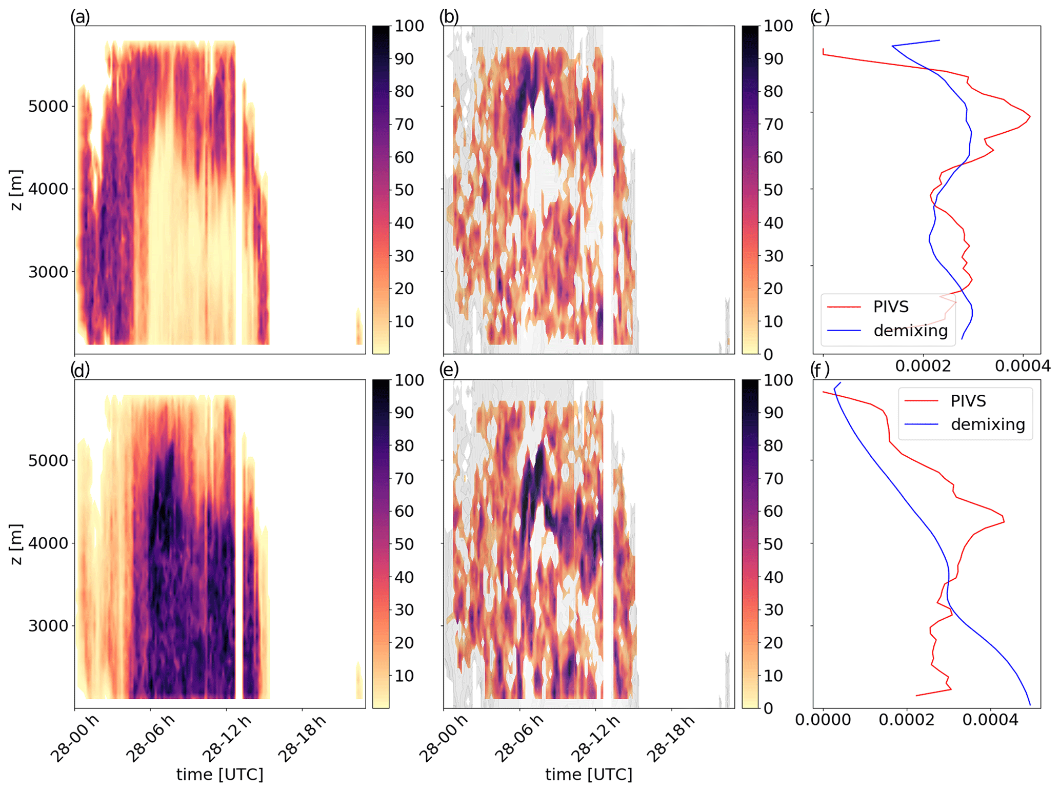
An additional comparison with hydrometeor proportions from the radar-based hydrometeor classification with demixing (Besic et al., 2018) provides complementary insights into the reliability and robustness of the PIVS method. One should, nonetheless, bear in mind that both the hydrometeor classification and the PIVS method are not completely independent since they are applied on the same radar data. However, the demixed hydrometeor proportions are determined based on the absolute values of the polarimetric variables within each individual radar volume (independently of the neighboring ones), while the PIVS method only relies upon the sign of the local vertical gradients. Importantly, the two methods do not give the same information. The demixing provides an estimate of the proportion of different hydrometeor types within a radar volume, whereas PIVS informs about the occurrence of microphysical processes along vertically neighboring radar volumes. The comparison between PIVS output and the demixing products is presented in Fig. 5 for EV1 and in Fig. 6 for EV2. In those two figures, the demixing generally exhibits high crystal (respectively, aggregate and rimed particle) concentrations where PIVS identifies CG (respectively, AR) as dominant. The difference between the two algorithms is highlighted in Figs. 5c and f and 6c and f, respectively, with the plot of the occurrence density for both the demixing and PIVSs (see the caption for details). A careful inspection of the averaged vertical distribution during the events (Figs. 5c, f and 6c, f) shows that CG (respectively, AR) generally occurs slightly above the maximum concentration in crystals (respectively, aggregates and rimed particles). This is consistent with the fact that the concentration of a given type of particle at a given height is mostly determined by the microphysical processes affecting the particles evolution earlier in time (i.e., higher in altitude).
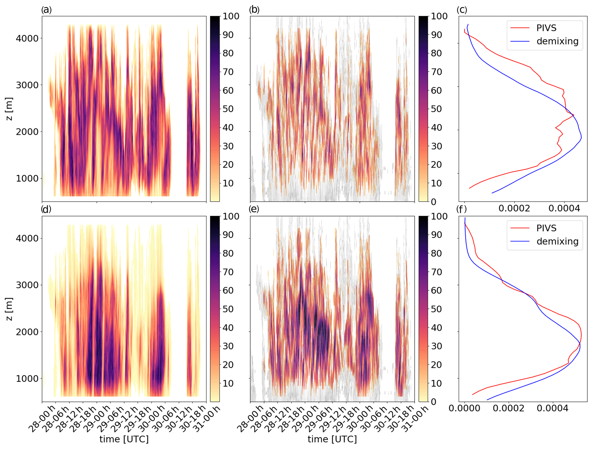
Figure 5Panel (a) (respectively, d) shows the time–height plot for EV1 of the proportion of crystals CR (respectively, aggregates AG and rimed particles RP) from the demixing algorithm. Panel (b) (respectively, e) shows the time–height plot of the proportion of CG (respectively, AR) from the PIVS method. Panel (c) (respectively, f) shows the vertical plots of the occurrence density of the CR demixed proportion and CG proportion during the event. The proportion for demixing is the number of counts for a specific hydrometeor divided by the total number of counts in this pixel and weighted by the proportion of profiles with significant signal at that height (i.e., with any process identified by PIVS) among all profiles. This enables a meaningful quantitative comparison between the two methods.
Moreover, one should remember that the radar sensitivity is lower at the top of the signal, and the PIVS outcome in the upper part of the clouds should, hence, be considered with caution.
Overall, the analysis of the PIVSs' products provides relevant insights into the microphysical processes governing snowfall, their occurrence and spatiotemporal organization. Section 4.5 uses this information to provide a statistical characterization of the considered microphysical processes.
4.5 Microphysical inferences from statistical analyses
We now gain further insights into the microphysics of the two case studies by carrying out a statistical analysis of the PIVSs' output. We use empirical conditional probabilities, defined as the probability ℙ of a variable C, taking the value c conditioned to a given process as follows:
At this point, it should be noted that PIVS characterizes the dominant processes in terms of radar signature. Because of the strong size dependence, a few large aggregates will dominate the radar signature quite rapidly compared to many more smaller ice crystals. Hence, one can expect that aggregation is detected as being a dominant process while CG persists, and the case is similar for SUB. This will moderate our analysis in the following section.
4.5.1 Mean height of process occurrence
Figure 7a shows the probability distribution of the altitude of occurrence for each process during EV1. SUB is the most frequent process between 500 and 1500 m a.g.l., while CG dominates between 2500 and 3500 m and AR prevails in between. Note that below 500 m no data are available, and above 4000 m, data might be affected by a decrease in the sensitivity of the radar. A clear statistical stratification in terms of dominant processes can be noticed. This stratification is also visible for EV2 (Fig. 8a), where CG mostly occurs between 4800 and 6000 m, AR between 4000 and 4800 m and SUB below. One should remember that, for EV2, the PIVS method was applied between 2000 m and 6000 m a.g.l. only.
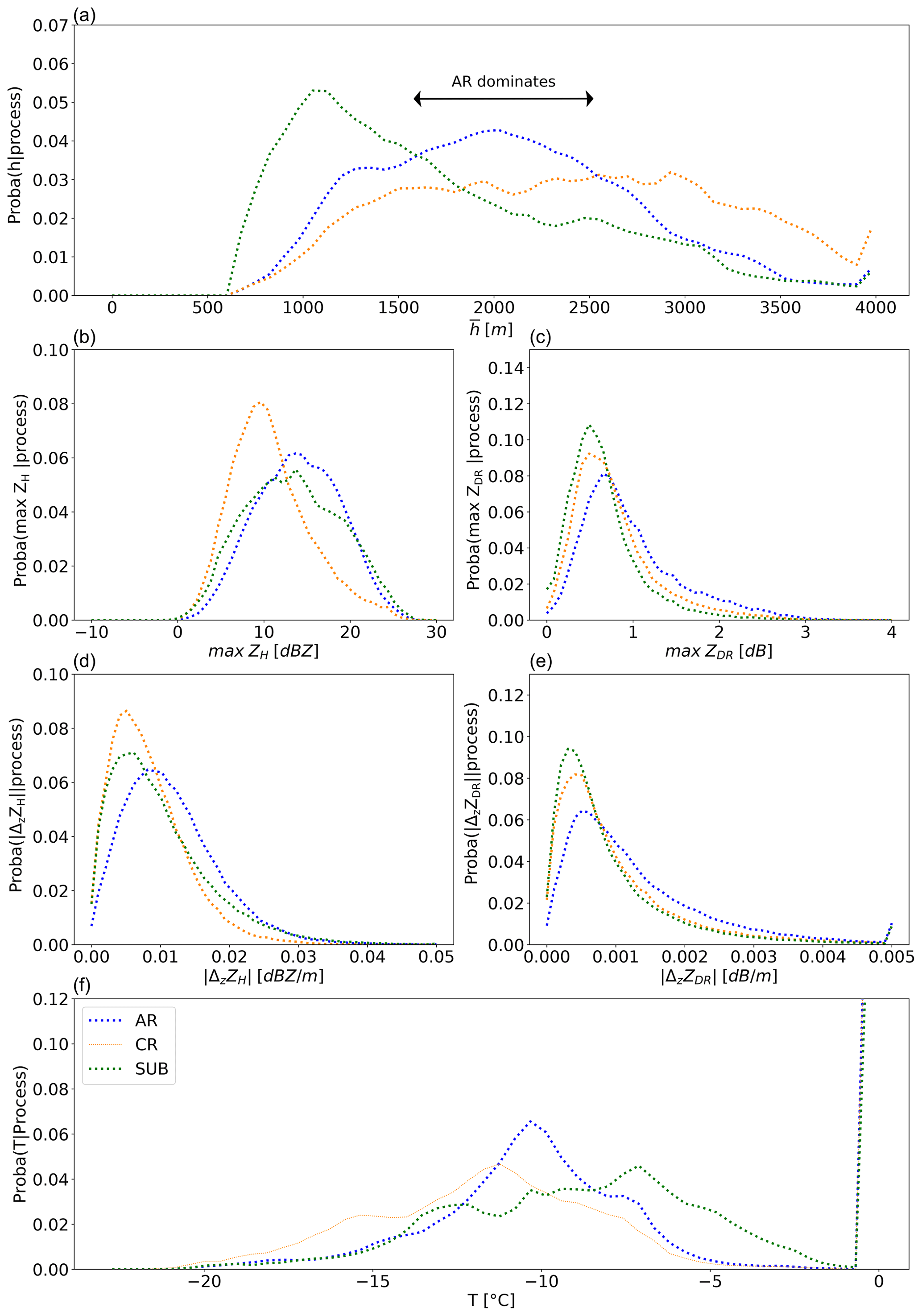
Figure 7Empirical conditional probability distributions for EV1. (a) Mean height of process occurrence a.g.l. . (b, c) Absolute maximal value of ZH and ZDR. (d, e) Absolute value of the mean local vertical gradient of ZH and ZDR. (f) Probability of temperature conditioned to different processes. The distributions are computed over all the sections of profiles identified as AR (blue), CG (orange) and SUB (green).

Although the vertical succession of the processes is similar between the two events, there is a clear difference in terms of absolute altitude values that can be explained by differences in temperature and humidity profiles driven by the synoptic circulation but also by more local aspects like the dry katabatic layer in Antarctica. The AR layer, however, has a similar thickness in the two distributions between 700 and 1000 m.
4.5.2 Magnitude and gradients of ZH and ZDR
Figure 7b (respectively, c) shows the distribution of the maximal values of ZH (respectively, ZDR) associated with a given process, over each vertical profile section during EV1 (maxZH and maxZDR). The three processes exhibit different signatures. AR shows the highest mean value for both maxZH and maxZDR. Moreover, the right tail of the maxZDR distribution is the highest for AR (only slightly for EV2; see Fig. 8c) and suggests that the highest values of ZDR – indicating large oblate particles – are mostly identified in AR regions. As AR is defined with positive upward gradients of ZDR, this suggests that crystals starting to aggregate or to rime first grow in size, density and oblateness and then progressively become less oblate as they continue to grow. This is consistent with the early aggregates signature proposed by Moisseev et al. (2015).
During EV2, one can distinguish two modes at around 11 and 20 dBZ in the distribution of maxZH for SUB (Fig. 8b). A close analysis of the output of PIVSs (not shown) reveals that the first mode corresponds to the sublimation layer below the warm front during its arrival above the radar (period during which ZH is relatively weak), whereas the second mode corresponds to elevated sublimation layers during the core of the event, when the reflectivity reaches higher values.
Figure 7d (respectively, e) shows the distribution of the local vertical gradient of ZH (respectively, ZDR) averaged over the sections of profiles corresponding to the different processes during EV1 (see Fig. 8d, e for EV2). During the two events, AR exhibits the largest and means but also the highest tails for . for SUB exhibits different statistical signatures between EV1 and EV2; the right tail of the distribution is the shortest among the three categories of processes during EV2 but comparable to that of AR and larger to that of CR during EV1. We believe this is explained by the strong katabatic winds during EV1 which are responsible for an enhanced sublimation. AR exhibits the largest gradients of both ZH and ZDR. Because AR and CG are both associated with positive downward relative gradients of ZH, it means that, on average, AR is more efficient at increasing the particle size (albeit decreasing its density) than CG. This result concurs with the fact that aggregation and riming are more efficient processes to increase the size of snowflakes than vapor deposition (Ryzhkov and Zrnić, 2019).
4.5.3 Temperature
Temperature is a key parameter influencing the occurrence of microphysical processes. It was, for instance, identified as a driving factor for aggregation efficiency (Hobbs et al., 1974; Connolly et al., 2012). Hobbs et al. (1974) distinguish two different preferential modes for aggregation at two temperatures, i.e., one associated with mechanical aggregation (dendrites that mechanically intricate with each other) and one with sticking aggregation at warmer temperatures (crystals that bound together thanks to their sticky melting surface).
Figures 7f and 8f present the normalized distribution of temperature after knowing a process for the two events. Temperature is obtained from WRF simulation (see Appendix A for details). For AR, EV2 presents two peaks, around −8 and −17 ∘C, while EV1 only shows a very well-defined peak at −10 ∘C. We suggest that the second peak for EV2 (coldest) and the peak for EV1 may correspond to the mechanical entanglement of aggregation described by Hobbs et al. (1974) and Connolly et al. (2012) (with a slight difference in temperature:; Hobbs et al. (1974) suggests a temperature range between −10 and −15 ∘C, and Connolly et al. (2012) observes a maximum in aggregation efficiency at −15 ∘C). However, riming cannot be disentangled from aggregation in AR, and it possibly influences these signatures. CG has a wider temperature distribution ranging from −7 to −17 ∘C during EV1 and from −5 to −21 ∘C during EV2. This is consistent with the theoretical models for vapor deposition with different growth habits, depending on supersaturation with respect to ice, and with temperature down to −38 ∘C (e.g., Nakaya, 1954; Libbrecht, 2005). The two signatures of SUB for both events are similar; they exhibit a maximum around −6 ∘C and a secondary mode at colder temperatures (−13 and for EV1 and EV2, respectively). The secondary mode is less accentuated for EV1, probably due to the katabatic layer that is responsible for an intense and continuous low-level sublimation above the Antarctic coast. The high temperature range, thus, corresponds to a low-level, very dry air where sublimation is the dominant microphysical process.
This study presents the development and application of a new method named PIVSs to automatically detect the occurrence of microphysical processes controlling snowfall growth and evolution from dual-polarization Doppler radar scans. PIVS is based on the analysis of the sign of the vertical gradients of ZH and ZDR extracted from RHI scans. A total of Three classes of microphysical processes (aggregation and/or riming, crystal growth by vapor deposition and sublimation) are identified by jointly observing the sign of the gradients along vertical profiles of the two variables. PIVS differs from hydrometeor classification methods that rely on the absolute value of polarimetric variables. It focuses instead on the vertical evolution of the characteristics of the particles with microphysical processes. In addition, it is insensible to calibration errors that can sometimes be an issue when using the ZDR quantity.
The environmental conditions in which the local vertical gradients of polarimetric signal primarily reflects the microphysical processes are first theoretically established. We derive three analytical conditions depending on the typical scales of spatiotemporal variations of the main variables shaping the radar signal (ZH, ZDR, u and vz). These conditions ensure that (i) the horizontal transport of ZH and ZDR is negligible with respect to its vertical evolution, (ii) the vertical divergence of (w−vz)ZH is mainly driven by the variation in ZH itself and not by variations in relative vertical velocity and (iii) the timescales of variations of ZH, and ZDR, due to microphysical processes, are sufficiently large so that the profiles of ZH and ZDR can reach a local quasi-equilibrium with the microphysical processes. These conditions, verified at the scale of the entire event, are sufficient conditions to reliably use PIVSs.
We apply and illustrate PIVSs on two frontal snowfall cases, i.e., one at Dumont d'Urville, Adélie Land, Antarctica, and one in the Taebaek mountains, South Korea. The robustness of the method is assessed by successfully comparing the output with two complementary data sets, namely snowflake observations from a MASC at the ground and products from a hydrometeor classification based on polarimetric radar data. This comparison highlights the local limitations of the method, especially in strong updrafts or fall streaks, i.e., when the three conditions, albeit respected over the bulk of the event, do not hold locally. We derive characteristic metrics of the microphysical processes, in particular the altitude of layers in which each process is dominant, and the vertical extension thereof. PIVS also allows us to characterize the statistics of radar variables (maxZH, maxZDR, and ) conditioned to the microphysical processes. Potential early aggregate signatures have, for instance, been identified and a complementary analysis of the processes' occurrence dependence on temperature shows signatures that may be associated to the onset of mechanical aggregation.
The present analysis could be easily replicated to other events in polar or mountainous environments sampled by a polarimetric radar, making it possible to better understand the processes governing the formation and evolution of snowfall in different meteorological contexts. Future methodological developments may include additional polarimetric variables, like Kdp, to help identify and distinguish additional processes (in particular secondary ice generation processes, i.e., Ryzhkov and Zrnić, 2019, or early aggregate generation, i.e., Moisseev et al., 2015). Finally, preliminary works not shown here have suggested that PIVSs'output can be useful for evaluating the ability of atmospheric models to reproduce the snowfall microphysical processes at the correct location and time. Such an application of the PIVS method would deserve further exploration in the future.
To gain access to the high-resolution spatiotemporal temperature field around the measurement sites and to complement the scale analysis in Sect. 4.2, we run numerical simulations with the 4.0 version of the Weather Research and Forecasting (WRF) model. The simulations setup is similar to the one presented in Vignon et al. (2019a). It consists of a downscaling method, where a 27 km resolution parent domain contains a 9 km resolution nest, which contains a 3 km resolution domain, which itself contains a 102×102 km2 nest centered over the measurement site (either DDU or GWU) at a 1 km resolution. To allow for a concomitant comparison with observations and to ensure realistic synoptic dynamics in the model, the wind field in the 27 and 9 km resolution domains has been nudged towards ERA5 reanalysis (Hersbach et al., 2020). The physical package is similar to the one of Vignon et al. (2019a). In particular, the two-moment (for rain, ice, snow and graupel categories) microphysical scheme from Morrison et al. (2005) is employed. In the following, as the snow particle size distribution is assumed to have an exponential shape, the kth moment of the distribution ,
can be calculated from the standard output of WRF, i.e., the snow mass mixing ratio QS [kg kg−1], and the number concentration NS [kg−1] is as follows:
In those equations, ρ is the air density, D is the particle dimension and (respectively, λS) is the intercept (respectively, slope parameter) of the size distribution. Unless otherwise mentioned, the analyzed model fields are those from the 1 km resolution domain.
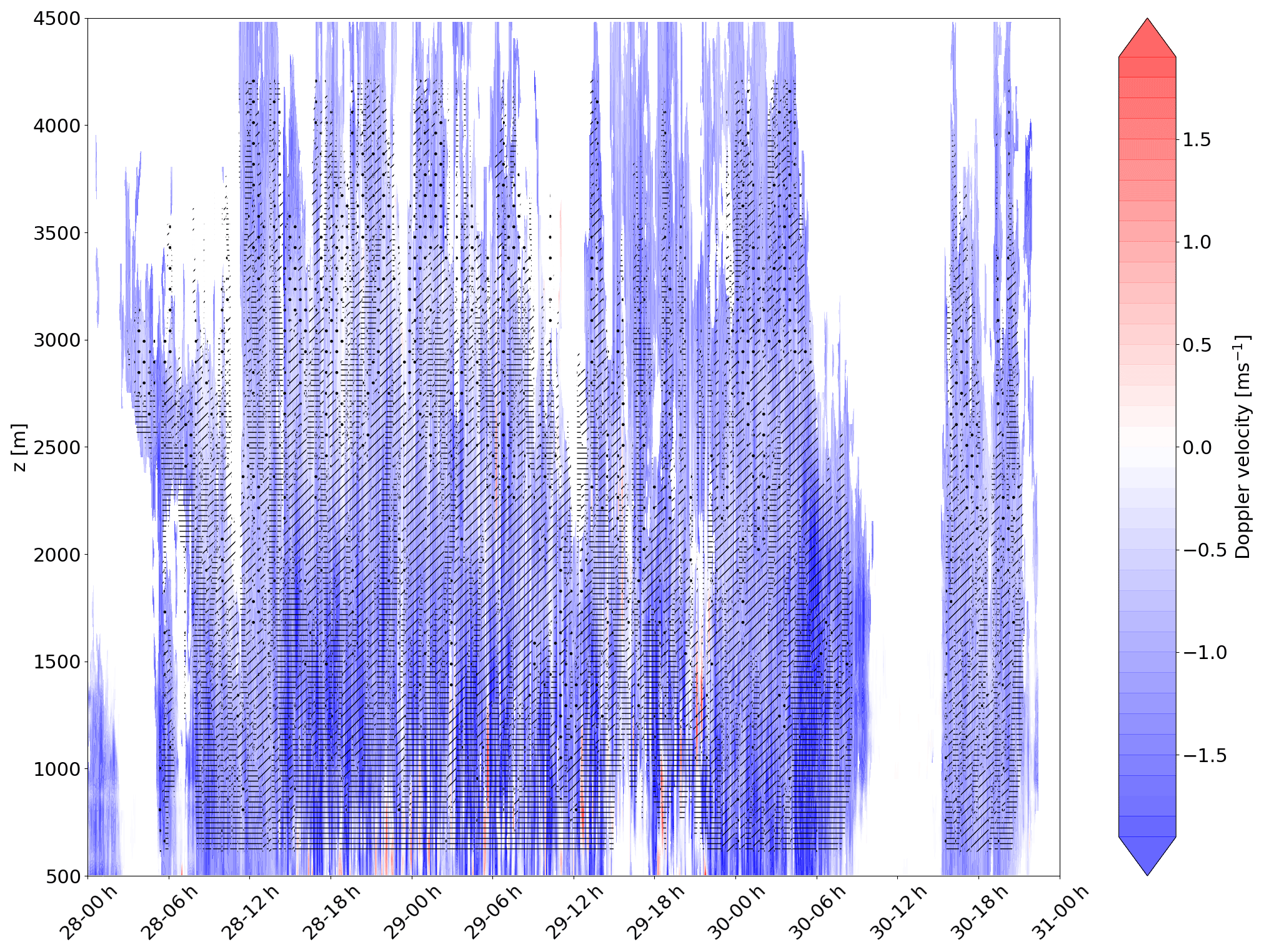
Figure A1Vertical Doppler velocity time–height plot during EV2 (WProf data). We superimpose the PIVS output, i.e., dots ∴ stand for CG, stand for AR and ≡ stand for SUB.
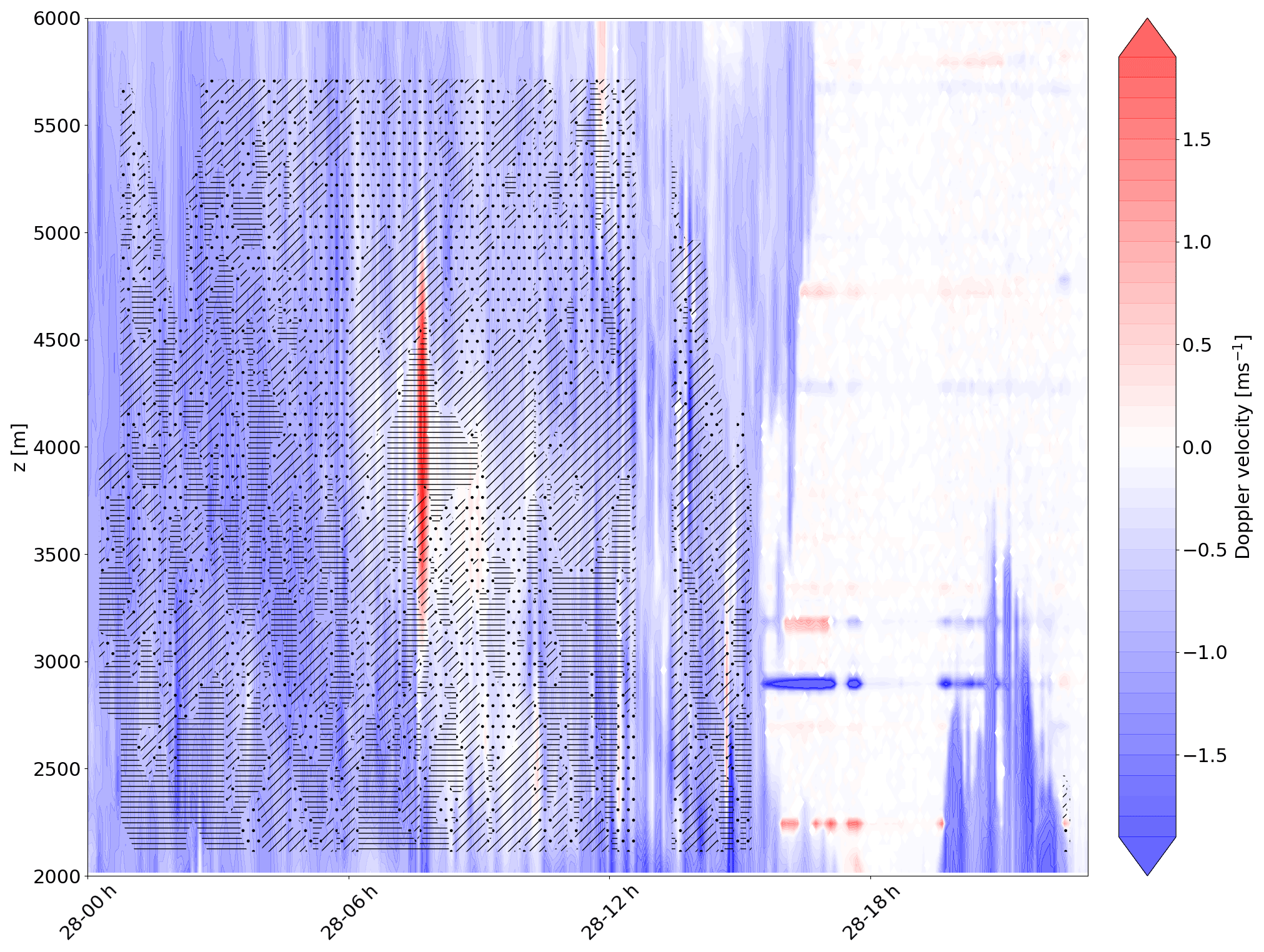
In strong turbulent updrafts, it can happen that the velocity of the particles becomes positive. In such conditions, as explained in Sect. 3.2, the criteria for identifying a microphysical process based on the sign of the vertical gradients of ZH and ZDR should be inverted.
In our data set, due to the instrumental configuration, we cannot retrieve the vertical Doppler velocity jointly with ZH and ZDR. During EV1, vertical velocity measurements are available strictly above the radar, in a region where we cannot estimate ZDR. During EV2, the cloud profiler WProf – which provides frequent Doppler velocity profiles – is located at MHS, 20 km away from MXPOL. Hence, we cannot precisely detect the regions where the vertical Doppler velocity is positive within RHIs scans.
By inspecting the time evolution of the Doppler velocities from the vertical profiles, we can pinpoint time periods during which we can expect the application of PIVSs not to be reliable. On the one hand, EV1 exhibits few updrafts visible in the vertical Doppler velocity time–height plots (see Fig. A2). These sparse updrafts are mainly located in the katabatic layer, which is more turbulent than the upper layers (e.g., Denby, 1999; Vignon et al., 2020) but remain limited in amplitude and temporal extent. On the other hand, during EV2, strong updrafts are observed between 07:00 and 09:00 UTC (see Fig. A1 and Gehring et al., 2020). These updrafts last longer than during EV1, and their vertical extent reaches almost 2000 m. The atmosphere above the Taebaek Mountains – and, thus, probably the one above MXPOL too – therefore experience a very unstable period, questioning the reliability of the PIVS method at this specific time.
Setting a radar profiler up within the RHI scan could help to accurately locate the turbulent and unstable regions and could provide interesting information about Doppler velocity characteristics for the three processes.
The APRES3 campaign data are freely distributed on the PANGAEA data repository (https://doi.org/10.1594/PANGAEA.883562; Berne et al., 2017). Further information on the ICE-POP data set and its distribution is given in Gehring et al. (2021, https://doi.org/10.5194/essd-13-417-2021).
The supplement related to this article is available online at: https://doi.org/10.5194/amt-14-4543-2021-supplement.
NP, JG, ÉV and AB designed and conducted the study. NP carried out the major part of the analysis. NP and JG processed the radar data. NP and EV derived the theoretical framework. EV ran the WRF simulations. NP prepared the paper, with contributions from all authors.
The authors declare that they have no conflict of interest.
We are grateful to Nikola Besic, for running the demixing algorithm over the two case studies. We are greatly appreciative of the participants of the World Weather Research Programme Research Development Project and Forecast Demonstration Project and the International Collaborative Experiments for Pyeongchang 2018 Olympic and Paralympic winter games (ICE-POP 2018) hosted by the Korea Meteorological Administration. We also acknowledge the support of the French National Research Agency (ANR) and the French Polar Institute (IPEV) for the APRES3 project (http://apres3.osug.fr, last access: 31 May 2021). We finally thank the two anonymous reviewers, who helped improve an earlier version of the paper.
Josué Gehring received financial support from the Swiss National Science Foundation (grant no. 175700/1). Étienne Vignon's contribution has been financed by the EPFL LOSUMEA project.
This paper was edited by Gianfranco Vulpiani and reviewed by two anonymous referees.
Andrić, J., Kumjian, M. R., Zrnić, D. S., Straka, J. M., and Melnikov, V. M.: Polarimetric signatures above the melting layer in winter storms: An observational and modeling study, J. Appl. Meteorol. Clim., 52, 682–700, 2013. a, b, c
Bader, M., Clough, S., and Cox, G.: Aircraft and dual polarization radar observations of hydrometeors in light stratiform precipitation, Q. J. Roy. Meteor. Soc., 113, 491–515, 1987. a
Berne, A., Grazioli, J., and Genthon, C. Precipitation observations at the Dumont d'Urville station, Adelie Land, East Antarctica, PANGAEA [data set], https://doi.org/10.1594/PANGAEA.883562, 2017. a
Besic, N., Figueras i Ventura, J., Grazioli, J., Gabella, M., Germann, U., and Berne, A.: Hydrometeor classification through statistical clustering of polarimetric radar measurements: a semi-supervised approach, Atmos. Meas. Tech., 9, 4425–4445, https://doi.org/10.5194/amt-9-4425-2016, 2016. a
Besic, N., Gehring, J., Praz, C., Figueras i Ventura, J., Grazioli, J., Gabella, M., Germann, U., and Berne, A.: Unraveling hydrometeor mixtures in polarimetric radar measurements, Atmos. Meas. Tech., 11, 4847–4866, https://doi.org/10.5194/amt-11-4847-2018, 2018. a, b, c
Browning, K., Hardman, M., Harrold, T., and Pardoe, C.: The structure of rainbands within a mid-latitude depression, Q. J. Roy. Meteor. Soc., 99, 215–231, 1973. a
Clough, S. and Franks, R.: The evaporation of frontal and other stratiform precipitation, Q. J. Roy. Meteor. Soc., 117, 1057–1080, 1991. a
Connolly, P. J., Emersic, C., and Field, P. R.: A laboratory investigation into the aggregation efficiency of small ice crystals, Atmos. Chem. Phys., 12, 2055–2076, https://doi.org/10.5194/acp-12-2055-2012, 2012. a, b, c
Denby, B.: Second-order modelling of turbulence in katabatic flows, Bound.-Lay. Meteorol., 92, 65–98, 1999. a
Durán-Alarcón, C., Boudevillain, B., Genthon, C., Grazioli, J., Souverijns, N., van Lipzig, N. P. M., Gorodetskaya, I. V., and Berne, A.: The vertical structure of precipitation at two stations in East Antarctica derived from micro rain radars, The Cryosphere, 13, 247–264, https://doi.org/10.5194/tc-13-247-2019, 2019. a, b
Garrett, T. J., Fallgatter, C., Shkurko, K., and Howlett, D.: Fall speed measurement and high-resolution multi-angle photography of hydrometeors in free fall, Atmos. Meas. Tech., 5, 2625–2633, https://doi.org/10.5194/amt-5-2625-2012, 2012. a
Gehring, J., Oertel, A., Vignon, É., Jullien, N., Besic, N., and Berne, A.: Microphysics and dynamics of snowfall associated with a warm conveyor belt over Korea, Atmos. Chem. Phys., 20, 7373–7392, https://doi.org/10.5194/acp-20-7373-2020, 2020. a, b, c, d, e, f, g, h, i, j, k
Gehring, J., Ferrone, A., Billault-Roux, A.-C., Besic, N., Ahn, K. D., Lee, G., and Berne, A.: Radar and ground-level measurements of precipitation collected by the École Polytechnique Fédérale de Lausanne during the International Collaborative Experiments for PyeongChang 2018 Olympic and Paralympic winter games, Earth Syst. Sci. Data, 13, 417–433, https://doi.org/10.5194/essd-13-417-2021, 2021. a, b
Genthon, C., Berne, A., Grazioli, J., Durán Alarcón, C., Praz, C., and Boudevillain, B.: Precipitation at Dumont d'Urville, Adélie Land, East Antarctica: the APRES3 field campaigns dataset, Earth Syst. Sci. Data, 10, 1605–1612, https://doi.org/10.5194/essd-10-1605-2018, 2018. a, b
Gorodetskaya, I. V., Kneifel, S., Maahn, M., Van Tricht, K., Thiery, W., Schween, J. H., Mangold, A., Crewell, S., and Van Lipzig, N. P. M.: Cloud and precipitation properties from ground-based remote-sensing instruments in East Antarctica, The Cryosphere, 9, 285–304, https://doi.org/10.5194/tc-9-285-2015, 2015. a
Grazioli, J., Lloyd, G., Panziera, L., Hoyle, C. R., Connolly, P. J., Henneberger, J., and Berne, A.: Polarimetric radar and in situ observations of riming and snowfall microphysics during CLACE 2014, Atmos. Chem. Phys., 15, 13787–13802, https://doi.org/10.5194/acp-15-13787-2015, 2015. a, b, c
Grazioli, J., Genthon, C., Boudevillain, B., Duran-Alarcon, C., Del Guasta, M., Madeleine, J.-B., and Berne, A.: Measurements of precipitation in Dumont d'Urville, Adélie Land, East Antarctica, The Cryosphere, 11, 1797–1811, https://doi.org/10.5194/tc-11-1797-2017, 2017a. a, b, c, d
Grazioli, J., Madeleine, J.-B., Gallée, H., Forbes, R., Genthon, C., Krinner, G., and Berne, A.: Katabatic winds diminish precipitation contribution to the Antarctic ice mass balance, P. Natl. Acad. Sci. USA, 114, 10858–10863, https://doi.org/10.1073/pnas.1707633114, 2017b. a, b
Green, J., Ludlam, F., and McIlveen, J.: Isentropic relative-flow analysis and the parcel theory, Q. J. Roy. Meteor. Soc., 92, 210–219, 1966. a
Griffin, E. M., Schuur, T. J., and Ryzhkov, A. V.: A Polarimetric Radar Analysis of Ice Microphysical Processes in Melting Layers of Winter Storms Using S-Band Quasi-Vertical Profiles, J. Appl. Meteorol. Clim., 59, 751–767, 2020. a
Harrold, T.: Mechanisms influencing the distribution of precipitation within baroclinic disturbances, Q. J. Roy. Meteor. Soc., 99, 232–251, 1973. a
Hersbach, H., Bell, B., Berrisford, P., Hirahara, S., Horányi, A., Muñoz-Sabater, J., Nicolas, J., Peubey, C., Radu, R., Schepers, D., Simmons, A., Soci, C., Abdalla, S., Abellan, X., Balsamo, G., Bechtold, P., Biavati, G., Bidlot, J., Bonavita, M., De Chiara, G., Dahlgren, P., Dee, D., Diamantakis, M., Dragani, R., Flemming, J., Forbes, R., Fuentes, M., Geer, A., Haimberger, L., Healy, S., Hogan, R. J., Hólm, E., Janisková, M., Keeley, S., Laloyaux, P., Lopez, P., Lupu, C., Radnoti, G., de Rosnay, P., Rozum, I., Vamborg, F., Villaume, S., and Thépaut, J.-N.: The ERA5 global reanalysis, Q. J. Roy. Meteor. Soc., 146, 1999–2049, 2020. a
Hobbs, P. V., Chang, S., and Locatelli, J. D.: The dimensions and aggregation of ice crystals in natural clouds, J. Geophys. Res., 79, 2199–2206, 1974. a, b, c, d
Jullien, N., Vignon, É., Sprenger, M., Aemisegger, F., and Berne, A.: Synoptic conditions and atmospheric moisture pathways associated with virga and precipitation over coastal Adélie Land in Antarctica, The Cryosphere, 14, 1685–1702, https://doi.org/10.5194/tc-14-1685-2020, 2020. a
Kalesse, H., Szyrmer, W., Kneifel, S., Kollias, P., and Luke, E.: Fingerprints of a riming event on cloud radar Doppler spectra: observations and modeling, Atmos. Chem. Phys., 16, 2997–3012, https://doi.org/10.5194/acp-16-2997-2016, 2016. a
Kennedy, P. C. and Rutledge, S. A.: S-band dual-polarization radar observations of winter storms, J. Appl. Meteorol. Clim., 50, 844–858, 2011. a
Küchler, N., Kneifel, S., Löhnert, U., Kollias, P., Czekala, H., and Rose, T.: A W-Band radar–radiometer system for accurate and continuous monitoring of clouds and precipitation, J. Atmos. Ocean. Tech., 34, 2375–2392, 2017. a
Kumjian, M. R.: The impact of precipitation physical processes on the polarimetric radar variables, PhD thesis, University of Oklahoma, available at: https://shareok.org/handle/11244/319188 (last access: 2 June 2021), 2012. a
Lebel, T. and Bastin, G.: Variogram identification by the mean-squared interpolation error method with application to hydrologic fields, J. Hydrol., 77, 31–56, 1985. a
Li, H., Moisseev, D., and von Lerber, A.: How does riming affect dual-polarization radar observations and snowflake shape?, J. Geophys. Res.-Atmos., 123, 6070–6081, 2018. a
Libbrecht, K. G.: The physics of snow crystals, Rep. Prog. Phys., 68, 855–895, 2005. a
Lubin, D., Zhang, D., Silber, I., Scott, R. C., Kalogeras, P., Battaglia, A., Bromwich, D. H., Cadeddu, M., Eloranta, E., Fridlind, A., Frossard, A., Hines, K. M., Kneifel, S., Leaitch, W. R., Lin, W., Nicolas, J., Powers, H., Quinn, P. K., Rowe, P., Russell, L. M., Sharma, S., Verlinde, J., and Vogelmann, A. M.: AWARE: The Atmospheric Radiation Measurement (ARM) West Antarctic Radiation Experiment, B. Am. Meteorol. Soc., 101, E1069–E1091, 2020. a
Milbrandt, J. and Yau, M.: A multimoment bulk microphysics parameterization. Part I: Analysis of the role of the spectral shape parameter, J. Atmos. Sci., 62, 3051–3064, 2005. a
Moisseev, D. N., Lautaportti, S., Tyynela, J., and Lim, S.: Dual-polarization radar signatures in snowstorms: Role of snowflake aggregation, J. Geophys. Res.-Atmos., 120, 12644–12655, 2015. a, b, c, d, e
Morrison, H., Curry, J. A., and Khvorostyanov, V. I: A New Double-Moment Microphysics Parameterization for Application in Cloud and Climate Models. Part I: Description, J. Atmos. Sci., 62, 1665–1677, https://doi.org/10.1175/JAS3446.1, 2005. a
Morrison, H., van Lier-Walqui, M., Fridlind, A. M., Grabowski, W. W., Harrington, J. Y., Hoose, C., Korolev, A., Kumjian, M. R., Milbrandt, J. A., Pawlowska, H., Posselt, D. J., Prat, O. P., Reimel, K. J., Shima, S.-I., van Diedenhoven, B., and Xue, L.: Confronting the challenge of modeling cloud and precipitation microphysics, J. Adv. Model. Earth Sy., 12, e2019MS001689, https://doi.org/10.1029/2019MS001689, 2020. a
Murphy, A. M., Ryzhkov, A., and Zhang, P.: Columnar vertical profile (CVP) methodology for validating polarimetric radar retrievals in ice using in situ aircraft measurements, J. Atmos. Ocean. Tech., 37, 1623–1642, 2020. a
Nakaya, U.: Snow crystals: natural and artificial, Harvard University Press, Harvard, Boston, MA, USA, https://doi.org/10.4159/harvard.9780674182769, 1954. a
Passarelli Jr., R. E.: An approximate analytical model of the vapor deposition and aggregtion growth of snowflakes, J. Atmos. Sci., 35, 118–124, 1978. a
Pfitzenmaier, L., Unal, C. M. H., Dufournet, Y., and Russchenberg, H. W. J.: Observing ice particle growth along fall streaks in mixed-phase clouds using spectral polarimetric radar data, Atmos. Chem. Phys., 18, 7843–7862, https://doi.org/10.5194/acp-18-7843-2018, 2018. a
Praz, C., Roulet, Y.-A., and Berne, A.: Solid hydrometeor classification and riming degree estimation from pictures collected with a Multi-Angle Snowflake Camera, Atmos. Meas. Tech., 10, 1335–1357, https://doi.org/10.5194/amt-10-1335-2017, 2017. a, b
Ryzhkov, A. and Zrnić, D. S.: Radar Polarimetry for Weather Observations, Springer, Cham, Switzerland, https://doi.org/10.1007/978-3-030-05093-1, 2019. a, b, c, d, e, f
Ryzhkov, A., Zhang, P., Reeves, H., Kumjian, M., Tschallener, T., Trömel, S., and Simmer, C.: Quasi-vertical profiles–A new way to look at polarimetric radar data, J. Atmos. Ocean. Tech., 33, 551–562, 2016. a
Scarchilli, C., Ciardini, V., Grigioni, P., Iaccarino, A., De Silvestri, L., Proposito, M., Dolci, S., Camporeale, G., Schioppo, R., Antonelli, A., Baldini, L., Roberto, N., Argentini, S., Bracci, A., and Frezzotti, M.: Characterization of snowfall estimated by in situ and ground-based remote-sensing observations at Terra Nova Bay, Victoria Land, Antarctica, J. Glaciol., 66, 1006–1023, https://doi.org/10.1017/jog.2020.70, 2020. a
Schaer, M., Praz, C., and Berne, A.: Identification of blowing snow particles in images from a Multi-Angle Snowflake Camera, The Cryosphere, 14, 367–384, https://doi.org/10.5194/tc-14-367-2020, 2020. a
Schneebeli, M., Dawes, N., Lehning, M., and Berne, A.: High-resolution vertical profiles of X-band polarimetric radar observables during snowfall in the Swiss Alps, J. Appl. Meteorol. Clim., 52, 378–394, 2013. a, b, c
Schrom, R. S. and Kumjian, M. R.: Connecting microphysical processes in Colorado winter storms with vertical profiles of radar observations, J. Appl. Meteorol. Clim., 55, 1771–1787, 2016. a
Scipión, D., Mott, R., Lehning, M., Schneebeli, M., and Berne, A.: Seasonal small-scale spatial variability in alpine snowfall and snow accumulation, Water Resour. Res., 49, 1446–1457, 2013. a
Shupe, M. D., Walden, V. P., Eloranta, E., Uttal, T., Campbell, J. R., Starkweather, S. M., and Shiobara, M.: Clouds at Arctic atmospheric observatories. Part I: Occurrence and macrophysical properties, J. Appl. Meteorol. Clim., 50, 626–644, 2011. a
Sinclair, V. A., Moisseev, D., and von Lerber, A.: How dual-polarization radar observations can be used to verify model representation of secondary ice, J. Geophys. Res.-Atmos., 121, 10954–10970, 2016. a
Skøien, J. O., Blöschl, G., and Western, A. W.: Characteristic space scales and timescales in hydrology, Water Resour. Res., 39, 1304, https://doi.org/10.1029/2002WR001736, 2003. a, b
Sotiropoulou, G., Vignon, É., Young, G., Morrison, H., O'Shea, S. J., Lachlan-Cope, T., Berne, A., and Nenes, A.: Secondary ice production in summer clouds over the Antarctic coast: an underappreciated process in atmospheric models, Atmos. Chem. Phys., 21, 755–771, https://doi.org/10.5194/acp-21-755-2021, 2021. a
Tiira, J. and Moisseev, D.: Unsupervised classification of vertical profiles of dual polarization radar variables, Atmos. Meas. Tech., 13, 1227–1241, https://doi.org/10.5194/amt-13-1227-2020, 2020. a, b
Vignon, E., Besic, N., Jullien, N., Gehring, J., and Berne, A.: Microphysics of Snowfall Over Coastal East Antarctica Simulated by Polar WRF and Observed by Radar, J. Geophys. Res.-Atmos., 124, 11452–11476, https://doi.org/10.1029/2019JD031028, 2019a. a, b, c, d, e
Vignon, É., Traullé, O., and Berne, A.: On the fine vertical structure of the low troposphere over the coastal margins of East Antarctica, Atmos. Chem. Phys., 19, 4659–4683, https://doi.org/10.5194/acp-19-4659-2019, 2019b. a, b
Vignon, É., Picard, G., Durán-Alarcón, C., Alexander, S. P., Gallée, H., and Berne, A.: Gravity wave excitation during the coastal transition of an extreme katabatic flow in Antarctica, J. Atmos. Sci., 77, 1295–1312, 2020. a
Wen, G., Oue, M., Protat, A., Verlinde, J., and Xiao, H.: Ice particle type identification for shallow Arctic mixed-phase clouds using X-band polarimetric radar, Atmos. Res., 182, 114–131, 2016. a
- Abstract
- Introduction
- When does microphysics drive the vertical variability?
- Development of the PIVS method
- Application of the methodology to two case studies
- Conclusions
- Appendix A: Numerical simulations with WRF
- Appendix B: Local unreliability of the method in case of strong turbulent updrafts
- Data availability
- Author contributions
- Competing interests
- Acknowledgements
- Financial support
- Review statement
- References
- Supplement