the Creative Commons Attribution 4.0 License.
the Creative Commons Attribution 4.0 License.
 | 21 Jan 2021
Ozone Monitoring Instrument (OMI) Aura nitrogen dioxide standard product version 4.0 with improved surface and cloud treatments
Lok N. Lamsal
Nickolay A. Krotkov
Alexander Vasilkov
Sergey Marchenko
Wenhan Qin
Eun-Su Yang
Zachary Fasnacht
Joanna Joiner
Sungyeon Choi
David Haffner
William H. Swartz
Bradford Fisher
Eric Bucsela
We present a new and improved version (V4.0) of the NASA standard nitrogen dioxide (NO2) product from the Ozone Monitoring Instrument (OMI) on the Aura satellite. This version incorporates the most salient improvements for OMI NO2 products suggested by expert users and enhances the NO2 data quality in several ways through improvements to the air mass factors (AMFs) used in the retrieval algorithm. The algorithm is based on the geometry-dependent surface Lambertian equivalent reflectivity (GLER) operational product that is available on an OMI pixel basis. GLER is calculated using the vector linearized discrete ordinate radiative transfer (VLIDORT) model, which uses as input high-resolution bidirectional reflectance distribution function (BRDF) information from NASA's Aqua Moderate Resolution Imaging Spectroradiometer (MODIS) instruments over land and the wind-dependent Cox–Munk wave-facet slope distribution over water, the latter with a contribution from the water-leaving radiance. The GLER combined with consistently retrieved oxygen dimer (O2–O2) absorption-based effective cloud fraction (ECF) and optical centroid pressure (OCP) provide improved information to the new NO2 AMF calculations. The new AMFs increase the retrieved tropospheric NO2 by up to 50 % in highly polluted areas; these differences arise from both cloud and surface BRDF effects as well as biases between the new MODIS-based and previously used OMI-based climatological surface reflectance data sets. We quantitatively evaluate the new NO2 product using independent observations from ground-based and airborne instruments. The new V4.0 data and relevant explanatory documentation are publicly available from the NASA Goddard Earth Sciences Data and Information Services Center (https://disc.gsfc.nasa.gov/datasets/OMNO2_V003/summary/, last access: 8 November 2020), and we encourage their use over previous versions of OMI NO2 products.
- Article
(28032 KB) - Full-text XML
- BibTeX
- EndNote


The Dutch–Finnish-built Ozone Monitoring Instrument (OMI) has been operating onboard the NASA EOS Aura spacecraft since July 2004 (Levelt et al., 2006, 2018). The primary objectives of OMI's mission are to continue the long-term record of total column ozone and to monitor other trace gases relevant to tropospheric pollution worldwide. Observations of sunlight backscattered from the Earth over a wide range of UV and visible wavelengths (∼ 260–500 nm) made by OMI allow for the retrieval of various atmospheric trace gases, including nitrogen dioxide (NO2). NO2 is a critically important short-lived air pollutant originating from both anthropogenic and natural sources. It is the principal precursor to tropospheric ozone and a key agent for the formation of several toxic airborne substances such as nitric acid (HNO3), nitrate aerosols, and peroxyacetyl nitrate. Satellite-based observations yield a global, self-consistent NO2 data record that can complement field measurements.
During more than 16 years of operation, OMI has provided a unique, practically uninterrupted daily NO2 data record that has been widely used for atmospheric research and applications, accentuating demands for accurate NO2 data products. The power of OMI to track NO2 pollution is demonstrated through observations of enhanced column amounts over polluted industrial areas (e.g., Boersma et al., 2011; Lamsal et al., 2013; Krotkov et al., 2016; Kim et al., 2016; Cai et al., 2018; Montgomery and Halloway, 2018), weekly patterns with significant reduction on weekends following energy usage (e.g., Ialongo et al., 2016), and seasonal patterns (e.g., van der A et al., 2008) that reflect changes in NOx emissions and photochemistry (e.g., Shah et al., 2020). Exploiting the close relationship between NOx emissions and tropospheric NO2 columns, OMI NO2 data have been used to detect and quantify the strength and trends of NOx emissions from power plants (Duncan et al., 2013; de Foy et al., 2015; Liu et al., 2019), ships (e.g., Vinken et al., 2014a), lightning (e.g., Pickering et al., 2016), soil (e.g., Vinken et al., 2014b), oil and gas production (e.g., Dix et al., 2020), forest fires (Schreier et al., 2014), and other area sources such as cities in the US (Lamsal et al., 2015; Lu et al., 2015; Kim et al., 2016), Europe (e.g., Zhou et al., 2012; Castellanos et al., 2012; Vinken et al., 2014a), Asia (Ghude et al., 2013; Goldberg et al., 2019a), and other world urban areas (Krotkov et al., 2016; Duncan et al., 2016; Montgomery and Halloway, 2018). OMI NO2 observations have frequently been used to evaluate chemical transport models (CTMs) (e.g., Herron-Thrope et al., 2010; Han et al., 2011; Hudman et al., 2012; Pope et al., 2015; Rasool et al., 2016), to study atmospheric NOx chemistry and lifetime (e.g., Lamsal et al., 2010; Beirle et al., 2011; Canty et al., 2015; Tang et al., 2015; Laughner and Cohen, 2019), and to infer ground-level NO2 concentrations (Lamsal et al., 2008; Gu et al., 2017), NO2 dry deposition (Nowlan et al., 2014; Geddes and Martin, 2017), and emissions of co-emitted gases including carbon dioxide (CO2) (Konovalov et al., 2016; Goldberg et al., 2019b; Liu et al., 2020).
Over the last decade, there have been considerable efforts to improve NO2 data quality from OMI and other satellite instruments (e.g., Boersma et al., 2018). Special emphasis has been placed on improving auxiliary information (e.g., a priori NO2 vertical profiles, surface reflectivity), particularly with respect to spatial and temporal resolution. For instance, the global OMI NO2 products are based on a priori NO2 profiles from relatively coarse-resolution (> 1.0∘ × 1.25∘) global CTM simulations (Boersma et al., 2011; Krotkov et al., 2017; Choi et al., 2020). Many regional studies suggest a general low bias in the global tropospheric NO2 column products, particularly over polluted areas, that can be partially mitigated by using a priori information from high-resolution CTM simulations (Russell et al., 2011; McLinden et al., 2014; Lin et al., 2014, 2015; Goldberg et al., 2017; Choi et al., 2020). Current global NO2 retrievals are based on a low-resolution (0.5∘ × 0.5∘) static climatology of the surface Lambert equivalent reflectivity (OMLER) product (Kleipool et al., 2008), which is likely biased high due to insufficient cloud and aerosol screening. This bias in surface reflectivity can lead to an underestimation of tropospheric NO2 retrievals (Zhou et al., 2010; Lin et al., 2014; Vasilkov et al., 2017). In addition, the OMLER data do not account for the significant day-to-day (orbital) variability in surface reflectance caused by changes in sun–satellite geometry, a phenomenon often expressed by the bidirectional reflectance distribution function (BRDF). Zhou et al. (2010) demonstrated the impact of both the spatial resolution and the BRDF effect on OMI tropospheric NO2 retrievals over Europe by using high-resolution surface BRDF and albedo products from the Moderate Resolution Imaging Spectroradiometer (MODIS). Taking advantage of the MODIS high-resolution data, albeit neglecting the BRDF and atmospheric effects, Russell et al. (2011) and McLinden et al. (2014) created improved NO2 products from the NASA standard product (Bucsela et al., 2013; Lamsal et al., 2014) over the continental US and Canada, respectively. While these and subsequent studies (e.g., Kuhlmann et al., 2015; Laughner et al., 2019) addressed the limitation of climatological LER data for NO2 retrievals, they did not account for the surface BRDF effect on the OMI cloud products (cloud pressure and fraction), which are also inputs to the NO2 algorithm. Applying the MODIS BRDF data consistently to both the NO2 and cloud retrievals demonstrably improves the quality of OMI NO2 retrievals over China (Lin et al., 2014, 2015; Liu et al., 2019). However, this approach is computationally expensive and is applicable to land surfaces only. Our previous work (Vasilkov et al., 2018) proposed an approach appropriate for satellite NO2 data processing on a global scale (a) by using MODIS BRDF information consistently in the cloud and NO2 retrievals (b) for both land and water and (c) in an efficient way. Here, we apply the approach globally for the first time in the standard NASA OMI NO2 algorithm.
In this paper we describe various updates made in the version 4.0 (V4.0) NASA OMI NO2 algorithm, discuss their impact on the retrievals of tropospheric and stratospheric NO2 column amounts, and provide an initial quantitative assessment of NO2 data quality. Section 2 describes the OMI NO2 algorithm and various auxiliary data used by the algorithm. We present validation results in Sect. 3. Section 4 summarizes the conclusions of this study.
OMI is an ultraviolet–visible (UV–Vis) spectrometer on the polar-orbiting NASA Aura satellite (Levelt et al., 2006, 2018). Aura, launched on 15 July 2004, follows a sun-synchronous orbit with an Equator crossing time near 13:45 local time. OMI employs two-dimensional charge-coupled device (CCD) detectors and operates in a push-broom mode, registering spectral data over a 2600 km cross-track spatial swath. The broad swath enables global daily coverage within 14–15 orbits. In the OMI visible channel used for NO2 retrievals, each swath, measured every 2 s, comprises 60 cross-track fields of view (FOVs) varying in size from ∼ 13 km × 24 km near nadir to ∼ 24 km × 160 km for the FOVs at the outermost edges of the swath. Each orbit consists of ∼ 1650 swaths from terminator to terminator. OMI's full daily coverage has been affected by data loss due to an anomaly presumably caused by material on the spacecraft outside the instrument that results in reduced coverage to about half of its original swath, as discussed in Sect. 2.4.
The OMI NO2 standard product (OMNO2) algorithm provides retrievals of NO2 column (total, tropospheric, and stratospheric) amounts by exploiting Level-1B calibrated radiance and irradiance data from the visible channel (350–500 nm with 0.63 nm spectral resolution). The algorithm employs a multi-step procedure that consists of (1) a spectral fitting algorithm to calculate NO2 slant column densities (SCDs) as discussed in Sect. 2.1, (2) determination of air mass factors (AMFs) to convert SCDs to vertical column densities (VCDs) as discussed in detail in Sect. 2.2, (3) a scheme to remove cross-track-dependent artifacts or stripes, and (4) a stratosphere–troposphere separation scheme to derive tropospheric and stratospheric NO2 VCDs. The AMF depends upon a number of parameters including optical geometry (solar and viewing azimuth and zenith angles), surface reflectivity, cloud pressure and fraction, and the shape of the NO2 a priori vertical profile.
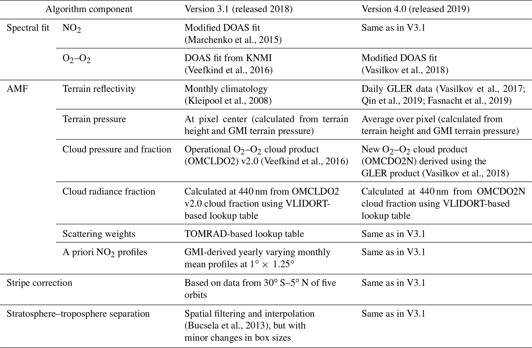
Since the first release of OMNO2 in 2006 (Bucsela et al., 2006; Celarier et al., 2008), there have been significant conceptual and technical improvements in the retrieval of NO2 from space-based measurements. Prior versions developed a new scheme for separating stratospheric and tropospheric components in version 2.1 (V2.1) (Bucsela et al., 2013; Lamsal et al., 2014) and a new algorithm for improved NO2 SCD retrievals in V3.0 (Marchenko et al., 2015; Krotkov et al., 2017), including improved cloud products (Veefkind et al., 2016) in V3.1 (Choi et al., 2020). The current version, V4.0, further improves on the retrievals in a number of significant ways for NO2 AMF and VCD calculations. Figure 1 shows a schematic diagram of the retrieval algorithm, and Table 1 summarizes the differences and similarities between previous (V3.1) and current (V4) versions. Some of the approaches in the V4 algorithm are similar to those used in V3.1, but there are several important changes as discussed in detail in Sect. 2.1 and 2.2.
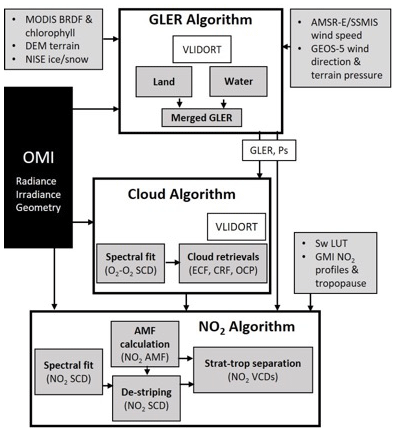
Figure 1Schematic diagram of the NASA OMI NO2 algorithm version 4.0, which is coupled with the cloud- and geometry-dependent surface Lambertian equivalent reflectivity (GLER) algorithms that ultimately produce stratospheric (strat) and tropospheric (trop) NO2 vertical column densities (VCDs). Acronyms used here are described in the relevant sections below. VLIDORT: vector linearized discrete ordinate radiative transfer; MODIS: Moderate Resolution Imaging Spectroradiometer; BRDF: bidirectional reflectance distribution function; DEM: digital elevation model; NISE: near-real-time ice and snow extent; AMSR-E: Advanced Microwave Scanning Radiometer for Earth Observing System (EOS); SSMIS: Special Sensor Microwave Imager–Sounder; GEOS-5: Goddard Earth Observing System version 5; Ps: surface (terrain) pressure over OMI pixel; ECF: effective cloud fraction; CRF: cloud radiance fraction; OCP: optical centroid pressure; Sw: scattering weight; LUT: lookup table; GMI: Global Modeling Initiative; AMF: air mass factor; SCD: slant column density.
Table 1Summary of algorithms and approaches used in the NASA NO2 algorithms versions 3.1 and 4.0.
2.1 NO2 and O2–O2 spectral fitting
2.1.1 NO2 spectral fitting algorithm
The spectral fitting algorithm for the operational standard OMI NO2 product is described in detail in Marchenko et al. (2015). Briefly, the algorithm retrieves NO2 slant column densities (SCDs) by using a differential optical absorption spectroscopy (DOAS) approach (e.g., Platt and Stutz, 2006). In the DOAS approach, laboratory-measured spectra of NO2 (Vandaele et al., 1998) and glyoxal (Volkamer et al., 2005), HITRAN08-based water vapor spectra (Rothman et al., 2009), and rotational Raman (RR; Ring effect) filling-in are sequentially fitted to the OMI-measured reflectance spectrum in the 402–465 nm wavelength range. The slant column represents the integrated abundance of NO2 along the average photon path from the sun through the atmosphere to the satellite. The Ring spectra are calculated as a linear combination of the atmospheric (Joiner et al., 1995) and liquid water (Vasilkov et al., 2002) RR spectra, convolved with the wavelength- and cross-track-dependent OMI transfer function (Dirksen et al., 2006). The algorithm employs a multi-step, iterative retrieval procedure for removal of the Ring and spectral under-sampling (Chance, et al., 2005) patterns as well as a low-order polynomial smoothing prior to estimation of SCDs for all interfering species. This is in contrast to the conventional DOAS approach that treats the Ring effect as a pseudo-absorber and fits all absorbers simultaneously with the polynomial functions. For accurate wavelength shifts (radiances vs. irradiances), the standard product algorithm splits the entire fitting window into seven carefully selected, partially overlapping micro-windows, iteratively evaluates the RR spectrum amplitudes, performs wavelength adjustments for each segment, and then iteratively retrieves the NO2, H2O, and glyoxal in the windows best suited for a particular trace gas species.
The OMI NO2 SCDs from the standard product were compared with improved SCD retrievals from the Quality Assurance for Essential Climate Variables (QA4ECV; http://www.qa4ecv.eu/, last access: 18 May 2020), BIRA-IASB's (Royal Belgian Institute for Space Aeronomy) QDOAS software (http://uv-vis.aeronomie.be/software/QDOAS/, last access: 18 May 2020), and the latest KNMI retrievals (van Geffen et al., 2015) and are shown to agree within 2 % (Zara et al., 2018). The typical NO2 SCD uncertainties amount to ∼ 0.8 × 10¹⁵ molec. cm−2, or 5 %–7 % in high-SCD areas and 15 %–20 % in low-SCD areas (Marchenko et al., 2015).
2.1.2 O2–O2 spectral fitting algorithm
The oxygen dimer (O2–O2) slant column fitting algorithm shares many features of the NO2 fitting algorithm and is described in detail in Vasilkov et al. (2018). It consists of a multi-step, iterative retrieval approach with three carefully selected micro-windows sampling the flanks and the core of the broad O2–O2 feature centered at 477 nm. The algorithm exploits OMI-measured reflectance spectra in the 451–496 nm range to determine the wavelength shifts and RR amplitudes. The Ring patterns are removed from the original OMI reflectances during the iterative adjustments for differences in the wavelength registration of radiances and irradiances. The O2–O2 slant columns are retrieved after removal of the NO2 and H2O absorptions estimated by the algorithm discussed in the previous section and of the ozone absorption using total ozone data from Veefkind et al. (2006). After removal of the interfering signals, the 477 nm O2–O2 absorption profile is carefully normalized to the adjacent O2–O2 absorption-free reflectance levels accounting for very different wavelength dependencies of surface reflectances over various geographical sites (e.g., the open-ocean and desert area), as described in Vasilkov et al. (2018). The normalized O2–O2 absorption profiles are then iteratively fitted with the temperature-dependent cross sections from Thalman and Volkamer (2013) over the 463–488 nm range to derive O2–O2 SCDs. These are used to estimate the cloud properties as discussed below in Sect. 2.2.2.
2.2 Improved air mass factor calculations
The AMF, which is defined as the ratio of SCD to VCD, is needed to calculate the retrieved NO2 VCD. Details of the AMF and its calculation are given in Palmer et al. (2001). The AMF for each FOV is calculated by combining altitude-dependent (z-dependent) scattering weights (w) computed with a radiative transfer model and a local a priori vertical NO2 profile shape (S), taken from a chemistry transport model:
For the tropospheric AMF, the integral extends from the surface to the tropopause, whereas the integral from the tropopause to the top of the atmosphere provides the stratospheric AMF. The scattering weight at a given altitude describes the sensitivity of the backscattered radiation to the abundance of the absorber at that altitude. For an optically thin absorber like NO2, scattering weights are a function of atmospheric scattering and are considered to be independent of the species' vertical distribution (Palmer et al., 2001). Factors affecting scattering weights include wavelength, optical geometry (solar and viewing azimuth and zenith angles), surface reflectivity, and cloud pressure and fraction. The wavelength dependence of scattering weights is accounted for by creating an average of scattering weights derived from the values at multiple wavelengths within the NO2 spectral fitting window. To compensate for the effect of the assumed constant NO2 temperature (220 K) in the NO2 SCD retrievals, the scattering weights are corrected for the atmospheric temperature effect using local climatological monthly temperature profiles as discussed in Bucsela et al. (2013). These profiles are based on the meteorological field from the Modern-Era Retrospective Analysis for Research and Applications (MERRA-2) (Gelaro et al., 2017).
The a priori NO2 profile shapes are computed from a monthly mean climatology of vertical NO2 profiles constructed from the Global Modeling Initiative (GMI) CTM simulation (Douglass et al., 2004; Strahan et al., 2007; Strode et al., 2015) driven by MERRA-2 meteorology. The spatial resolution of the model is 1.25∘ in longitude and 1.0∘ in latitude, and the atmosphere is divided into 72 pressure levels extending from the surface to 0.01 hPa. The model output is sampled between 13:00 and 14:00 local time, consistent with the OMI overpass time. The use of monthly NO2 profiles helps capture the seasonal variation in the NO2 vertical distribution (Lamsal et al., 2010). The simulation is based on yearly varying NOx emissions, as discussed in Strode et al. (2015); this is necessary to account for the effect of rapidly changing NOx emissions (e.g., Tong et al., 2015; Duncan et al., 2016; Miyazaki et al., 2017) on local NO2 profile shapes (Lamsal et al., 2015; Krotkov et al., 2017).
For each FOV, AMFs are computed for clear (AMFclr) and cloudy (AMFcld) conditions. The AMF of a partially cloudy scene is calculated by assuming the independent pixel approximation:
where fr is the cloud radiance fraction (CRF), defined as the fraction of the measured radiation that comes from clouds and scattering aerosols, and it is computed at 440 nm from the retrieved effective cloud fraction (ECF), fc, using Eq. (8) (see below). AMFclr is calculated for the ground reflectivity of Rs and at terrain pressure Ps, whereas AMFcld is calculated assuming a Lambertian surface of reflectivity 0.8 at the retrieved cloud pressure. Below we provide a detailed discussion of each of these input parameters that are incorporated in the OMNO2 V4.0 algorithm.
2.2.1 New surface reflectivity product for NO2 and cloud retrievals
Surface reflectivity is an important input parameter for UV–Vis satellite retrievals of trace gases and cloud information. The surface reflectance over both ocean and land depends upon viewing and illumination geometry and can be accurately described by the bidirectional reflectance distribution function (BRDF). This effect is, however, neglected by most currently available trace gas and cloud algorithms, which use a climatological Lambert equivalent reflectivity (LER) for the surface. To account for surface BRDF effects in the NO2 and cloud retrievals, here we use the geometry-dependent surface LER (GLER) product derived using the Moderate Resolution Imaging Spectroradiometer (MODIS) BRDF data and the vector linearized discrete ordinate radiative transfer (VLIDORT) calculation (Vasilkov et al., 2017; Qin et al., 2019; Fasnacht et al., 2019). The GLER allows for a computationally efficient approach that does not require major changes to the existing trace gas and cloud algorithms.
We derive GLER by inverting the top-of-atmosphere (TOA) radiance (I) of a Rayleigh atmosphere over a non-Lambertian surface for each specific FOV and sun–satellite geometry within the Lambertian framework, i.e.,
where I0 is the TOA radiance calculated for a black surface, T is the total (direct + diffuse) solar irradiance reaching the surface converted to the ideal Lambertian-reflected radiance (by dividing by π steradians) and then multiplied by the transmittance of the reflected radiation between the surface and TOA in the direction of a satellite instrument, and Sb is the diffuse flux reflectivity of the atmosphere for the case of its isotropic illumination from below (Dave, 1978). The values of I0, T, and Sb are pre-computed with VLIDORT and stored in a lookup table. The GLER values are calculated at wavelengths relevant for both NO2 (440 nm) and cloud (466 nm) retrievals.
Over land, the BRDF is calculated using the Ross-thick Li-sparse kernel model (Lucht et al., 2000) in VLIDORT (Spurr, 2006):
where the coefficients aiso, avol, and ageo come from the Moderate Resolution Imaging Spectroradiometer (MODIS) Collection 5 gap-filled seasonally snow-free BRDF product MCD43GF (Schaaf et al., 2002, 2011) for band 3 (459–479 nm) available at 30 arcsec spatial resolution and 8 d temporal resolution. The term aiso is the isotropic contribution describing the Lambertian part of light reflection from the surface; the volumetric kernel (kvol) describes light reflection from a dense leaf canopy, and the geometric kernel (kgeo) describes light reflection from a sparse ensemble of surface objects casting shadows on the background assumed to be Lambertian. The kernels are the only angle-dependent functions, the expressions of which are given in Lucht et al. (2000). The band 3 BRDF coefficients spatially averaged over an actual satellite FOV are used to calculate TOA radiance and GLER at 466 nm. To calculate GLER at 440 nm, we apply a scaling method using the ratio of OMI-derived Lambert equivalent reflectivity (LER) data at 440 and 466 nm:
The value of is taken from the gridded monthly LER ratio data at 1∘ × 1∘ or coarser resolution. The LER is determined from OMI TOA radiance measurements as discussed in Vasilkov et al. (2017, 2018). We use clear-sky (effective cloud fraction < 0.02) and aerosol-free (OMI UV aerosol index, < 0.5; Torres et al., 2007) OMI LER data to create the monthly gridded data. The cloud and aerosol screening is necessary because the spectral dependence of surface features differs from that of clouds and aerosols.
Over water, the surface reflectance is calculated at the two wavelengths, 440 and 466 nm, using VLIDORT. To calculate TOA radiance, we include light specularly reflected from a rough water surface and diffuse light backscattered by water bulk. We also account for contributions from oceanic foam that can be significant for high wind speeds. Reflection from the water surface is described by the Cox–Munk slope distribution function, which depends on both the wind speed and the wind direction (Cox and Munk, 1954). Polarization at the ocean surface is accounted for by using a full Fresnel reflection matrix as suggested by Mishchenko and Travis (1997).
We use wind speed data from a pair of satellite microwave imagers that include the Advanced Microwave Scanning Radiometer–Earth Observing System (AMSR-E) instrument onboard the NASA Aqua satellite (Meissner and Wentz, 2004) for 2004–2011 and the Special Microwave Imager–Sounder (SSMIS) onboard the Air Force Defense Meteorological Satellite Program (DMSP) Satellite F16 (Wentz et al., 2012) afterwards. Wind direction data are taken from the Global Modeling Assimilation Office (GMAO) Goddard Earth Observing System Model Forward Processing for Instrument Teams (GEOS-5 FP-IT) near-real-time assimilation.
Diffuse light from the ocean is described by a Case 1 water model with a single input parameter of chlorophyll concentration (Morel, 1988) taken from the monthly Aqua MODIS data. The common Case 1 water model developed for the visible channel (Morel, 1988) was extended to the UV using data from Vasilkov et al. (2002, 2005). To calculate water-leaving radiance, we require the downwelling irradiance at the surface (i.e., atmospheric transmittance). Since the transmittance and the water-leaving contribution are coupled, we develop a simple coupling scheme in VLIDORT to ensure that the value of water-leaving radiance used as an input at the ocean surface will correspond to the correct value of the downwelling flux reaching the surface interface (Fasnacht et al., 2019).
For OMI ground pixels covering land and water surfaces, the TOA radiance (I) is calculated as an average of radiance for land (IL) and water (Iw) weighted by the pixel land fraction (f):
The value of f is determined by converting various surface categories in the MODIS data (note that these are of much higher spatial resolution than the OMI data) into a binary land–water mask (e.g., treating all shorelines and ephemeral water as the land category and classifying all other water subcategories simply as water). The areal fraction of land (or water) for each OMI pixel is then computed as the statistics of the binary categories.
Figure 2 shows an example of changes in surface reflectivity used in the previous (V3.1) and the current (V4.0) version of the OMI NO2 algorithm. The GLER data computed for OMI observations as discussed above for 20 March 2005 differ considerably from the OMI-derived climatological monthly LER data (Kleipool et al., 2008) for March. As shown in Figs. 2 and 3a, the GLERs are generally lower than climatological LER data except at swath edges with large viewing angles and over areas affected by sun glint that correspond to higher values of GLER. Changes over the sun-glint areas are rather large, reaching up to 0.3. The climatological LER data derived by analyzing histograms of 5 years of OMI-based LER data likely overestimate the actual surface reflectivity due to residual cloud and aerosol contamination and underestimate over sun-glint areas as the procedure ignores sun-glint-affected observations. In contrast, the GLER data over land are based on atmospherically corrected radiances from high-resolution MODIS observations, minimizing the impact of both cloud and aerosols.
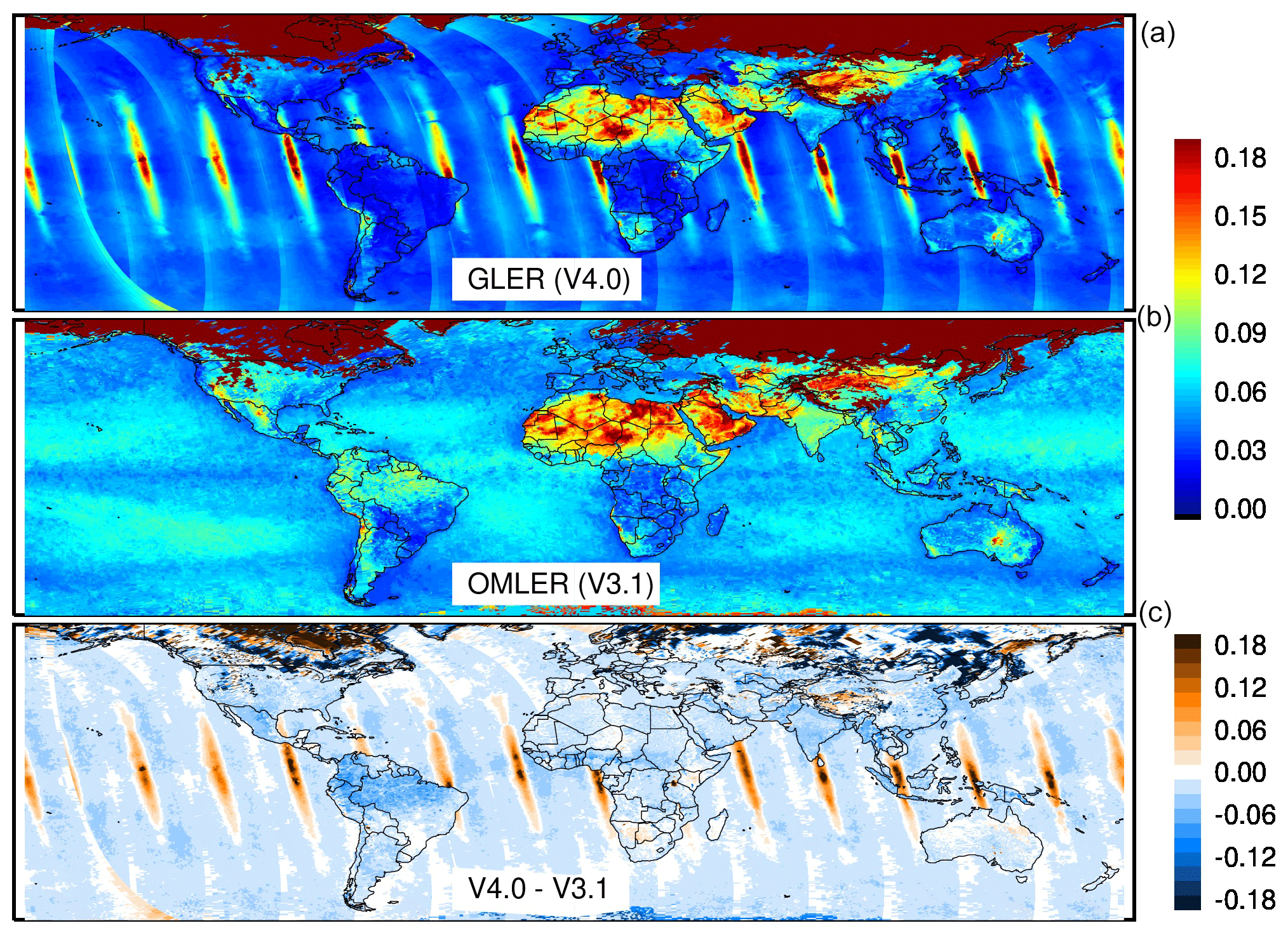
Figure 2Surface reflectivity at 440 nm (a) derived using MODIS BRDF data with OMI geometry (GLER) on 20 March 2005 compared with (b) OMI-based monthly LER climatology (OMLER) for the month of March (Kleipool et al., 2008). The bottom panel (c) shows the difference between MODIS-based and climatological surface reflectivity data.
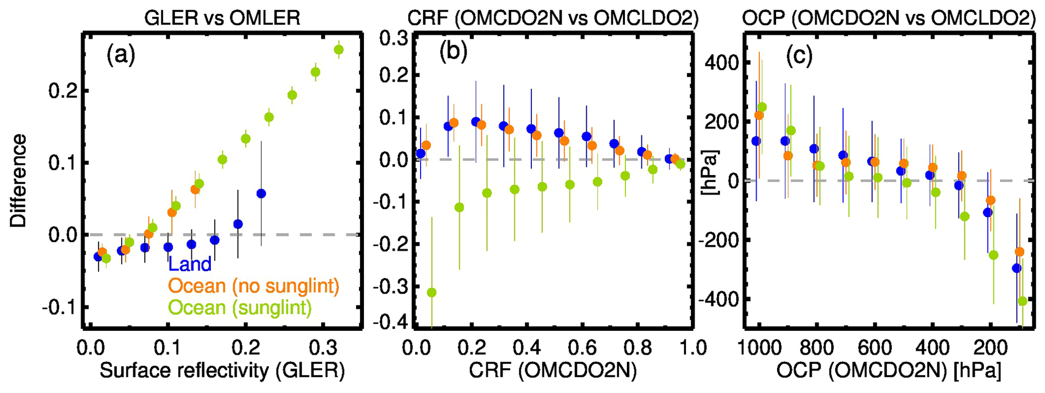
Figure 3Differences (V4.0–V3.1) in (a) surface reflectivity, (b) cloud radiance fraction, and (c) cloud optical centroid pressure for 20 March 2005, as used in the V3.1 and V4.0 algorithms and binned by the values of corresponding parameters from V4.0. Data are separated for land (blue) and ocean surfaces, as well as by sun-glint (green) and non-sun-glint (orange) geometry over ocean. The vertical bars represent the standard deviation for each bin of those parameters.
2.2.2 Improved cloud product retrieval
We develop a new algorithm that provides cloud parameters, namely cloud radiance fraction (CRF) and cloud optical centroid pressure (OCP), and use them in the OMNO2 algorithm. Similar to the standard OMCLDO2 algorithm (Veefkind et al., 2016), our cloud algorithm exploits the O2–O2 absorption to retrieve O2–O2 SCD as discussed in Sect. 2.1.2, but it derives the two cloud parameters using the GLER and other ancillary data that are used in the NO2 algorithm, maintaining inter-algorithm consistency. The OMCLDO2 algorithm retrieves these parameters using the climatological LER data from Kleipool et al. (2008). In the following, our new cloud product is referred to as OMCDO2N.
The derivation of CRF and OCP is based on a simple cloud model called the mixed Lambertian equivalent reflectivity (MLER) model (Joiner and Vasilkov, 2006; Veefkind et al., 2016). The MLER model treats cloud and ground as horizontally homogeneous, opaque Lambertian surfaces and mixes them using the independent pixel approximation (IPA). According to the IPA, the measured TOA radiance, Im, is a sum of the clear-sky (Ig) and overcast (Ic) subpixel TOA radiances that are weighted with an effective cloud fraction (ECF), fc (e.g., Stammes et al., 2008):
We choose the wavelength of 466 nm that is not substantially affected by rotational Raman scattering (RRS) or atmospheric absorption to derive fc. The parameters Ig and Ic are a function of the ground and cloud LERs, respectively, and are calculated using VLIDORT (Spurr, 2006) and obtained with an interpolated lookup table. We use GLER discussed above for ground reflectivity and a uniform cloud reflectivity of 0.8 (Koelemeijer et al., 2001; Stammes et al., 2008). The value of fc is calculated by inverting Eq. (7). Note that aerosols are implicitly accounted for in the determination of fc, as they are treated (like clouds) as particulate scatters. CRF (fr) defines the fraction of TOA radiance reflected by cloud:
We use pre-computed lookup tables of the TOA radiances generated using VLIDORT. Due to its wavelength dependence, we calculate CRF at 466 nm for OCP at 440 nm for NO2 retrievals.
The MLER model compensates for photon transport within a cloud by placing the Lambertian surface somewhere in the middle of the cloud instead of at the top (Vasilkov et al., 2008). The pressure of this surface corresponds to OCP, which can be modeled as a reflectance-averaged pressure level reached by backscattered photons (Joiner et al., 2012). We retrieve cloud OCP from the O2–O2 SCD discussed above (Sect. 2.1.2). The cloud OCP, Pc, is estimated by inversion using the MLER method to compute the appropriate O2–O2 AMFs:
where VCD (SCD ∕ AMF) is the vertical column density of O2–O2 over ground (VCDg) and cloud (VCDc). The clear-sky (AMFg) and overcast or cloudy (AMFc) subpixel AMFs are calculated at 477 nm with ground (GLER) and cloud (0.8) reflectivity, respectively. Lookup tables for the AMFs were generated using VLIDORT. Temperature profiles needed for estimation of VCD and AMF are taken from the GEOS-5 global data assimilation system (Rienecker et al., 2011).
In addition to OCP, we retrieve the so-called scene pressure. The scene pressure is derived from Eq. (9) assuming that fr=1 and cloud reflectivity equals the scene LER. The scene LER is determined from the measured TOA radiance using the equation (Eq. 3) that defines TOA radiance in the Rayleigh atmosphere over a Lambertian surface. In the absence of clouds, aerosols, and any major gas absorptions, the scene pressure should be equal to the surface pressure. The scene pressure is therefore an important diagnostic tool for evaluation of the performance of cloud pressure algorithms.
Figure 4 shows an example of cloud products retrieved with our algorithm compared with those retrieved from the standard OMCLDO2 algorithm (Veefkind et al., 2016). The retrieved OCP and CRF from the two algorithms exhibit broadly consistent spatial patterns in both cloud altitude and amount. The values of OCP generally range from 370 to 1001 hPa in OMCDO2N versus 150 to 1011 hPa in OMCLDO2N. For both products, CRF varies from 0 for clear-sky to 1 for overcast conditions. A systematic difference is evident, with generally higher values in OMCDO2N for OCP by 147 hPa and CRF by 0.01 compared to OMCLDO2. For OCP, there is a general pattern in difference, with OMCDO2N OCP higher for low-altitude clouds (> 700 hPa) and lower values for high-altitude clouds (< 300 hPa) (Fig. 3c). The largest OCP differences occur for cases in which cloud pressures in OMCLDO2 are clipped to 150 hPa. For CRF, larger differences occur for partially cloudy scenes, with higher CRF values in OMCDO2N by 0–0.1 for both land and water surfaces (Fig. 3b). Exceptions are over sun-glint areas where CRF in OMCDO2N is lower by 0–0.3 with a mean difference of 0.13.

Figure 4Cloud optical centroid pressure at 477 nm (a, c, e) and cloud radiance fraction at 440 nm (b, d, f) retrieved for 20 March 2005 with the OMNO2 V4.0 (a, b) and V3.1 (c, d) algorithms, respectively. Panels (e, f) show their differences. Gray represents the OMI pixels with retrieved cloud pressure equal to terrain pressure in V4.0 on the left and over snow and ice surface identified by the NISE flag on the right.
2.2.3 Treatment over snow and ice surfaces
Over ice and snow surfaces, identified by near-real-time ice and snow extent (NISE) flags (Nolin et al., 2005) in the OMI Level-1b data, the following treatments are made for surface reflectivity. In the case of permanent ice and snow surfaces, the MCD43GF product provides BRDF parameters, allowing us to calculate GLER. Over seasonal snow area usually with data gaps in MCD43GF, we calculate OMI-derived LER capped by a constant snow albedo of 0.6 following Boersma et al. (2011). In rare cases of pixels not flagged by NISE and gaps in MODIS data, we use OMI LER climatology (Kleipool et al., 2008) regardless of whether the surface is either snow- and ice-covered but missed by NISE or snow- and ice-free.
The OMI-derived scene reflectivity and scene pressure are used for NO2 and cloud retrievals over seasonally snow-covered areas. If the NISE flags are set as true, the following assumptions are made in our CRF, OCP, and NO2 retrievals. Over bright surfaces (scene reflectivity > 0.2), we consider the scenes to be snow- or cloud-covered and assign the scene pressure to OCP. In addition, if the difference between the surface pressure and scene pressure is smaller than 100 hPa, the scene is considered to be either cloud-free or covered by optically thin clouds following the cloud over snow classification by Vasilkov et al. (2010), and CRF for the pixel is set to zero. If the difference between the surface pressure and scene pressure exceeds 100 hPa, the scene is considered to be overcast by optically thick (shielding) clouds (Vasilkov et al., 2010), and CRF for the pixel is set to 1. To avoid a possible NISE misclassification (Cooper et al., 2018) for low-reflectivity scenes (scene reflectivity < 0.2), we consider such scenes to be snow- and ice-free and calculate CRF, OCP, and NO2 AMF using the standard procedure with GLER for those scenes.
2.2.4 Improved terrain height and pressure calculation
Terrain pressure is a critical parameter for the AMF in NO2 and cloud algorithms as well as for the total optical depth of the Rayleigh atmosphere in the GLER algorithm. Prior studies have shown that errors in terrain pressure can introduce over 20 % errors in retrieved NO2 VCD, especially in areas of complex terrain (Zhou et al., 2010; Russell et al., 2011).
Here, we use a 2 arcmin global relief model of global land–water surface data (ETOPOv2; National Geophysical Data Center, 2006) to derive terrain height for each individual OMI ground pixel. We derive the pixel-average terrain height by collocating and averaging the high-resolution data as discussed in Qin et al. (2019). The corresponding terrain pressure for each OMI pixel (Ps) is calculated from the terrain pressure–height relationship established based on MERRA-2 monthly terrain pressure (Ps_GMI) at a spatial resolution of 1∘ latitude × 1.25∘ longitude used in the GMI model discussed above:
where Δz () represents the difference between the average terrain height for an OMI pixel (z) and the terrain height at GMI resolution (zGMI). The parameter represents the scale height, where k is the Boltzmann constant, T is the temperature at the surface, M is the mean molecular weight of air, and g is the acceleration due to gravity.
2.3 Impact of the changes on AMF
Figure 5 shows an example of how changes in each individual input parameter affect tropospheric AMFs, which, in turn, translate inversely to tropospheric NO2 column retrievals. Replacing climatological LER from OMLER with daily GLER data affects scattering weight profiles in the lower troposphere, resulting in lower values of tropospheric AMF almost everywhere, except over sun-glint areas where the use of GLER enhances scattering weights and tropospheric AMF (Fig. 5a). The changes in tropospheric AMF with GLER usually range from −50 % to 25 %, occasionally reaching up to −100 %. The effect is small (−6 % to 1 %) for overcast scenes (CRF > 0.9), increases (−28 % to 17 %) over clear and partially cloudy scenes (CRF < 0.5) for unpolluted regions, and surges (−62 % to 3 %) over polluted areas ( molec. cm−2). Figure 6a shows GLER-driven changes in clear-sky (CRF < 0.5) tropospheric AMF for different surface and scene types, separated by tropospheric NO2 column amounts. For 80 % of cases over land, 97 % over water outside sun-glint areas, and 98 % over sun-glint areas, tropospheric NO2 columns are molec. cm−2, and the average GLER-driven differences are small at %, %, and 4.0±12.9 %, respectively. The differences increase gradually with column amount over NOx source regions (e.g., cities and highly polluted coastal areas), with binned (of size 1×10¹⁵ molec. cm−2) average differences ranging from % to %. Over snow and ice surfaces, changes are rather large, reaching up to a factor of 2. The impact of change in the surface reflection data on stratospheric AMFs is negligible (< 2 %).
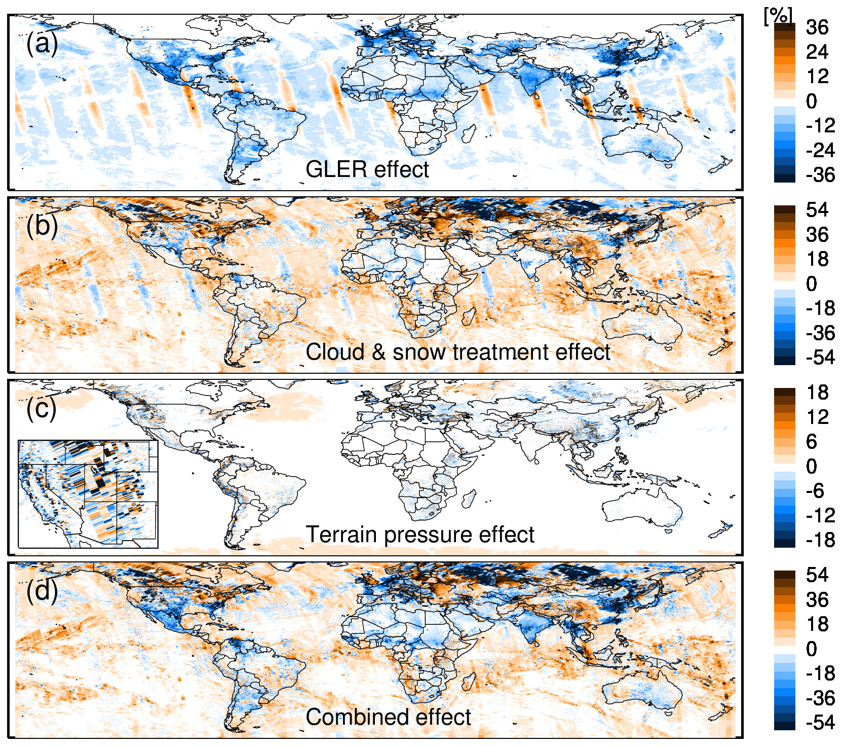
Figure 5Impact on tropospheric AMF (i.e., V4.0–V3.1) from changes in (a) surface reflectivity, (b) cloud and surface treatment, (c) terrain pressure, and (d) their combination on 20 March 2005. The panel (c) inset shows a zoomed view of the impact over complex terrain in the western US.
Figures 5b and 6b show how changes in the cloud parameters (CRF and OCP) affect tropospheric AMF. Replacing OMCLDO2-based cloud parameters with those from OMCDO2N changes scattering weight profiles in a complicated way. Higher values of OCP in OMCDO2N will include additional portions of scattering weights between the OMCDO2N- and OMCLDO2-based OCPs, especially in the lower troposphere, thereby reducing the tropospheric AMF. On the other hand, the higher CRF values lead to an increased contribution of the cloudy AMF in the calculation of tropospheric AMF, thereby increasing its value. Their combination causes a wide range of scenarios and large variation in the AMF effect. Overall, the change in cloud parameters causes enhancement of tropospheric AMFs for partially cloudy and overcast scenes and reduction for clear-sky scenes, especially over polluted areas. The AMF differences are generally large for low AMF values that are driven by enhanced differences in either OCP, CRF, or both as discussed in Vasilkov et al. (2017). The changes in tropospheric AMF with the OMCDO2N-based cloud parameters usually range from −17 % to 28 %, with larger variation over land (−34 % to 40 %) compared to water (−12 % to 25 %) and for low (< 1) AMF (−47 % to 41 %) compared to high (> 3) AMF (−4 % to 18 %). The largest changes in AMF (−96 % to 62 %) occur over snow and ice surfaces that result from the difference in the treatment of snow and ice for cloud and NO2 retrievals as discussed in Sect. 2.2.3. For clear-sky and partially cloudy scenes with CRF < 0.5, the effect of the changes in cloud parameters differs between land and water surfaces as well as sun-glint and non-sun-glint geometries and becomes more pronounced over polluted land and coastal areas (Fig. 6b). As in the case of surface reflectivity, the impact of the change in cloud parameters on stratospheric AMF is < 1 %.
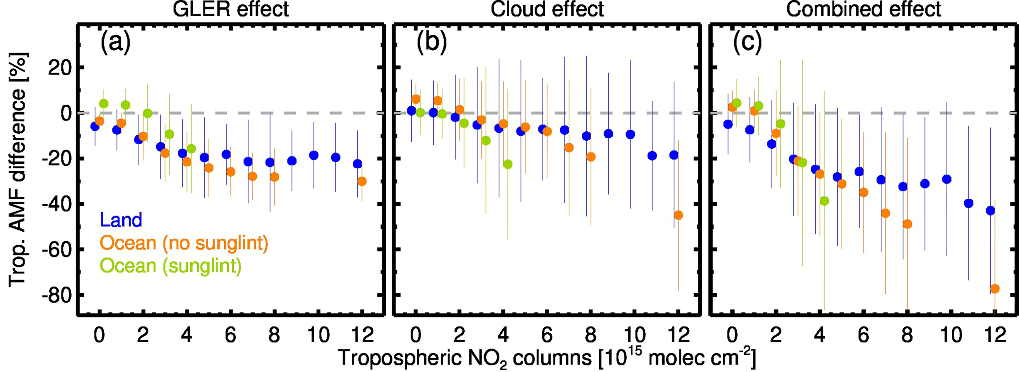
Figure 6The impact on tropospheric AMF (i.e., V4.0–V3.1) from changes in (a) surface reflectivity, (b) cloud, and (c) their combination for clear and partially cloudy scenes (CRF < 0.5) on 20 March 2005. Percent differences in tropospheric AMF are sorted by tropospheric NO2 columns, separating them by land (blue) and ocean, as well as by sun-glint (green) and non-sun-glint (orange) geometry over ocean. The vertical bars represent the standard deviations for the tropospheric NO2 column bins.
Figure 5c presents an example of changes in tropospheric AMF differences between the previous approach of using terrain pressure at OMI pixel centers and the pixel-average terrain pressure implemented in the current version (V4.0). In general, the AMF changes driven by the changes in terrain pressure are within ±1 % over ocean and ±3 % over land, although at times they can reach up to 30 %, especially for observations over complex terrain such as mountainous regions (Fig. 5c inset).
Figures 5d and 6c show the AMF differences arising from the combined effect of changes in all parameters discussed above. The effect arising from the replacement of the climatological OMLER with GLER is partially compensated for by the effect arising from the change in cloud parameters in places where the two parameters exhibit opposite trends. Exceptions are over polluted land and coastal areas; the GLER effect on AMF is augmented by the cloud effect. The average AMF changes arising from all parameters (2 %) are lower than the changes arising from either GLER (−2.3 %) or cloud parameters (4.1 %), although the combined effect leads to a wider range of variation in AMF changes (−100 % to 57 %) compared to the effect from individual parameters. The changes arising from all parameters are somewhat smaller (−21 % to 34 %) for overcast scenes (CRF > 0.9) compared to (−47 % to 29 %) clear and partially cloudy scenes (CRF < 0.5) and are substantial (−137 % to 30 %) over highly polluted areas ( molec. cm−2) and over snow and ice surfaces (−126 % to 99 %). Differences in the AMF effect are evident among land, water, and sun-glint areas (Fig. 6c). The impact of the changes is below 1 % for the stratospheric AMF.
2.4 Row anomaly and removal of stripes
The retrieved NO2 SCDs have persistent relative biases in the 60 cross-track FOVs and show a pattern of stripes running along each orbital track. This instrumental artifact is corrected using the “de-striping” procedure described in detail in Bucsela et al. (2013). Briefly, the de-striping algorithm estimates the mean cross-track biases using measurements obtained at latitudes between 30∘ S and 5∘ N and from orbits within two orbits of the target orbit. These correction values, one for each cross-track position, are then subtracted from the retrieved SCDs to derive the de-striped SCD field.
Starting 25 June 2007 and presumably even earlier, OMI experienced a more severe form of anomaly that affects the quality of radiance data in certain rows at all wavelengths (Dobber et al., 2008; Schenkeveld et al., 2017). This effect, called the “row anomaly” (RA), has developed and changed over time. Currently, the RA has affected approximately half of the OMI's FOVs, resulting in OMI's global coverage now being 2 d instead of 1 d before the onset of the RA.
The quality of radiance data for the RA-affected FOVs is sufficiently poor as to prevent reliable NO2 retrievals. Therefore, we abandon retrieval calculations for all measurements that are flagged by the RA-detection algorithm used in the Level-1 processing. We found that this RA-detection algorithm may not be sufficiently sensitive to the relatively small (but important for our purposes) RA changes. Figure 7 shows an example of anomalous rows not flagged by the RA-detection algorithm but observed in the NO2 retrievals. Shown are time series of average NO2 SCDs normalized by geometric AMFs over the Pacific Ocean for the RA-unaffected row of 20 (0-based) compared with three rows that show significant degradation in the quality of SCD retrievals. These particular rows are in immediate proximity to the main RA area, thus showing the gradual RA evolution: in the present epoch the RA slowly shifts towards the high-numbered rows – note the sequential timing of the big drops in the retrievals in rows 44–46. While the data from the three rows start deviating from row 20 beginning from summer 2016, the data quality degrades further for rows 44, 45, and 46 from September of 2017, 2018, and 2019, respectively, to the extent that they cannot be sufficiently corrected by the de-striping algorithm. In such cases, we implement additional RA flagging for those rows that start showing anomalous behavior and exclude those data from Level-2 and higher-level NO2 products.
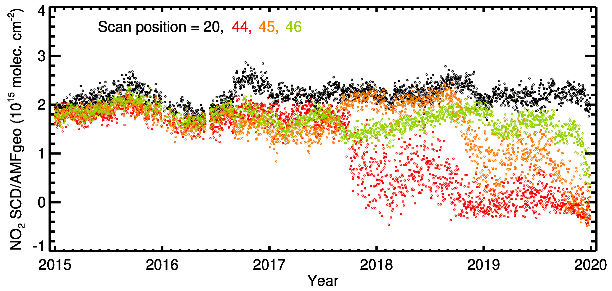
Figure 7The time series of OMI NO2 SCD normalized by the geometric AMF for clear-sky and partially cloudy conditions (CRF < 0.5) over the Pacific Ocean. The data are separated by cross-track scan position, comparing the presumably RA-free row 20 (black) with rows 44 (red), 45 (orange), and 46 (green). The row numbers are 0-based.
2.5 Calculation of stratospheric and tropospheric NO2 columns
We use an observation-based stratosphere–troposphere separation scheme to estimate the stratospheric NO2 field, as discussed in detail in Bucsela et al. (2013), and the algorithm remains unchanged in the current version. Briefly, the stratospheric field for an orbit is computed by creating a gridded global field of initial stratospheric NO2 VCD estimates (Vinit) with data assembled from within ±7 orbits of the target orbit:
Here, Sstrat and AMFstrat represent stratospheric SCD and AMF, respectively. A priori estimates of the tropospheric contribution () are subtracted from the measured de-striped SCDs (S), and grid cells wherein this contribution exceeds 0.3×10¹⁵ molec. cm−2 are masked. This masking ensures that the model contribution to the retrieval is minimal, especially in polluted areas. The residual field of the initial stratospheric VCDs measured outside the masked regions mainly over unpolluted or cloudy areas is smoothed by a boxcar average and a two-dimensional interpolation, yielding an estimate for stratospheric NO2 VCD (Vstrat) for an individual ground pixel.
The estimation of the stratospheric NO2 VCD allows for the computation of the tropospheric NO2 VCD (Vtrop) from the de-striped NO2 SCD (S) and the tropospheric AMF (AMFtrop):
where stratospheric NO2 SCD (Sstrat) is calculated from stratospheric AMF (AMFstrat) and Vstrat computed in the previous step.
With the updates in surface and cloud treatments as discussed in Sect. 2.2, the current version has made significant improvements, particularly in tropospheric AMFs and consequently in VCD estimates. Further improvement to the retrievals is possible by enhancing the quality of a priori NO2 profiles through improvements in model resolution, emissions, and chemistry, which remain unchanged in the current version. If improved a priori NO2 profiles become available, one can first use Eq. (1) to readily recalculate AMFtrop by combining them with scattering weights (w(z)) archived in the data files and then use Eq. (12) together with other supplied parameters to recalculate Vtrop. The same approach can be applied to remove the effect of a priori profiles used in retrievals altogether, while comparing NO2 columns from a model simulation with retrievals (Eskes and Boersma, 2003; Lamsal et al., 2014).
Figure 8 shows a comparison of tropospheric and stratospheric NO2 columns retrieved from the V3.1 and V4.0 algorithms for 20 March 2005. As expected, the updates implemented in V4.0 yield higher (∼ 10 %–40 %) tropospheric NO2 columns in polluted areas, with less-pronounced (±10 %) differences in background and low-column areas. These results are consistent with the observed differences in the tropospheric AMF as discussed above in Sect. 2.2.4 and with other previous regional studies over land surfaces (Zhou et al., 2010; McLinden et al., 2014; Lin et al., 2014, 2015; Laughner et al., 2019; Liu et al., 2019) that implemented one or more of the changes applied in V4.0. In contrast to changes in tropospheric NO2 retrievals, changes in stratospheric NO2 estimates range between molec. cm−2 and 3.2×10¹⁴ molec. cm−2 and are close to the range of expected uncertainties of stratospheric NO2 estimates (Bucsela et al., 2013). The relative differences in the stratospheric NO2 column between the two versions are close to 0 % on average, usually ranging between −2.5 % and 2.0 % and occasionally reaching up to ±13 %. This difference in stratospheric NO2 estimates is much larger than the difference in stratospheric AMFs and is caused by differences in tropospheric AMFs that influence NO2 observations over unpolluted and cloudy areas used by the stratosphere–troposphere separation scheme.
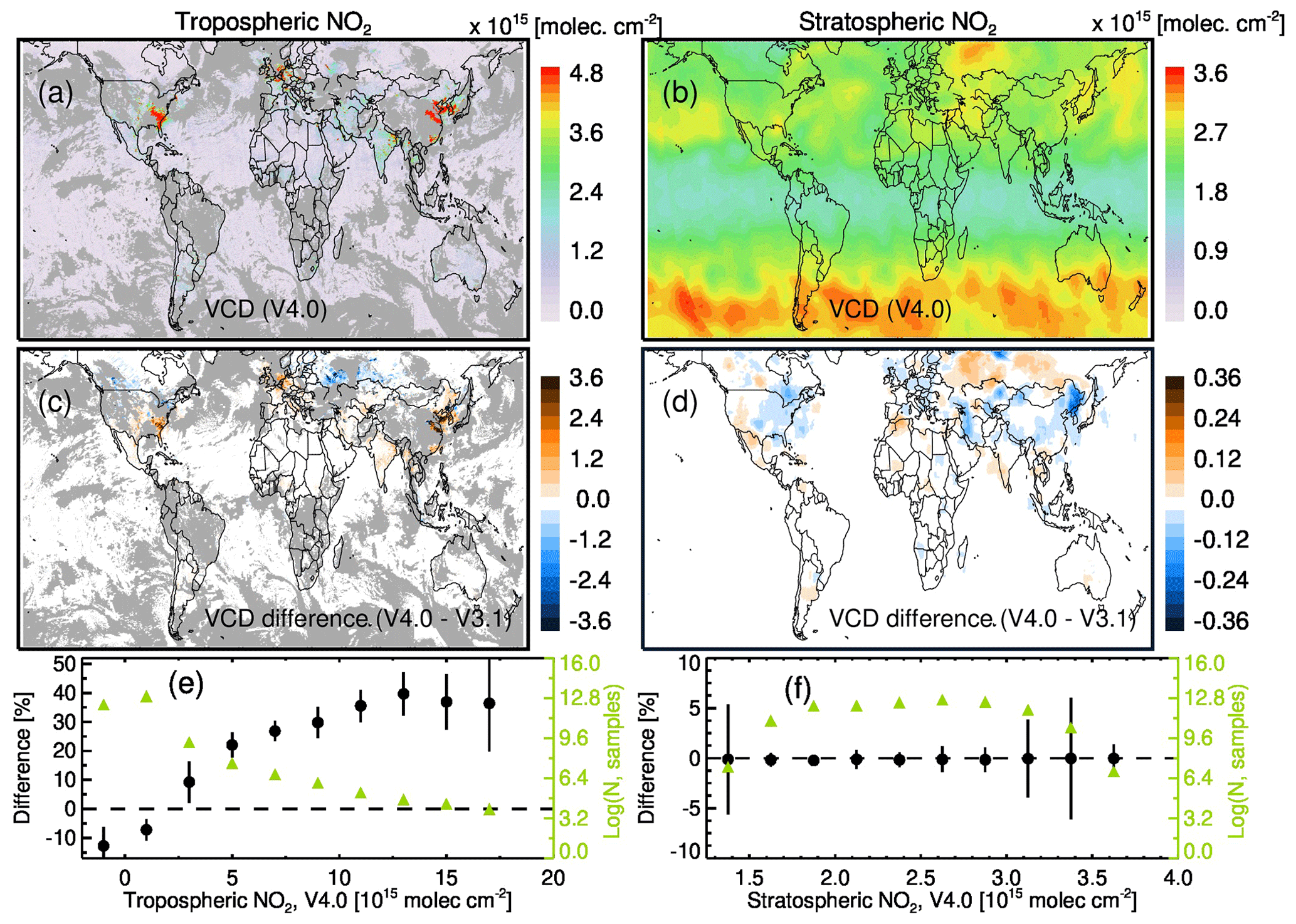
Figure 8Tropospheric (a) and stratospheric (b) NO2 VCD from V4.0 and their differences (c, d) with respect to V3.1 data (V4.0–V3.1) for 20 March 2005. Gray in the tropospheric NO2 maps represents cloudy areas (CRF > 0.5). Bottom panels show the average (black circles) and standard error (vertical bars) of the relative difference, 100 × (V4.0–V3.1) ∕ V3.1, for tropospheric (e) and stratospheric (f) NO2 VCDs plotted as a function of the respective NO2 column amounts. The green symbols represent the logarithm of the number of samples.
Figure 9 shows the seasonally averaged tropospheric NO2 columns over the selected domains of North America, Europe, southern Africa, and Asia for the months of June, July, and August in 2005. These domains contain highly polluted areas with significant NOx emissions where the impact of changes in surface reflectivity and cloud parameters on tropospheric NO2 retrievals becomes increasingly important. The use of more accurate pixel-specific information for surface and cloud parameters in V4.0 results in significantly enhanced tropospheric NO2 column retrievals almost everywhere. The effect, however, varies with the vertical distribution of NO2, with the largest effects in high-column areas.
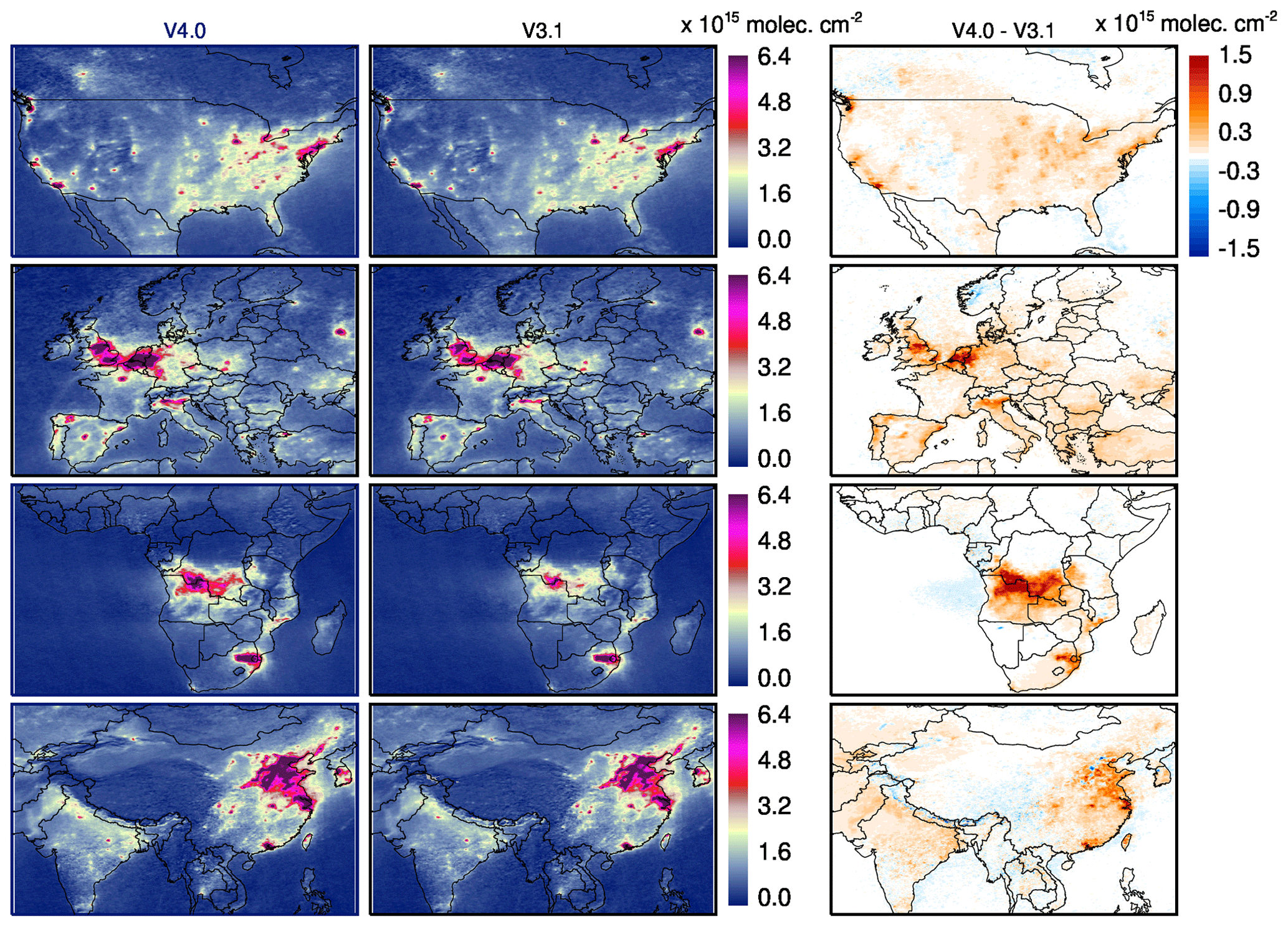
Figure 9The 3-month (June, July, August) average tropospheric NO2 columns for low cloud conditions (CRF < 0.5) in 2005 over North America (first row), Europe (second row), southern Africa (third row), and Asia (fourth row) from V4.0 (first column), V3.1 (second column), and their difference (V4.0–V3.1).
Figure 10 shows the seasonal average tropospheric NO2 columns for December through February. While seasonal differences in NO2 columns are evident owing to changes in NOx lifetime and boundary layer depth, the impact of algorithm changes in V4.0 remains similar. There are two notable exceptions specifically related to observations over snow and ice surfaces. First, there are significant data gaps in V3.1 but nearly none in V4.0. In V3.1, retrievals over snow and ice areas were considered to be highly uncertain and therefore discarded, following the recommendation of Boersma et al. (2011). As discussed above in Sect. 2.2.3, V4.0 incorporates changes in surface and cloud treatment in the NO2 algorithm that allows us to retain more observations that we determine to be our acceptable level of cloudiness. Next, these algorithm changes led to profound changes in the calculated tropospheric AMFs and resulting NO2 column amounts. The reduction in tropospheric NO2 retrievals in V4.0 over snow- and ice-covered surfaces arises from a combined effect of enhanced values of surface reflectivity, their impact on the CRF and OCP retrievals, and an inconsistent number of samples used in the calculation of the seasonal average. Nevertheless, due to inferiority in the quality of BRDF data and complexities in separating snow from clouds, caution is needed when interpreting wintertime data at high latitudes.

Figure 10Same as Fig. 9, but for December, January, and February. The gray areas represent a lack of good observations as determined by data quality flags.
Figure 11 shows some examples of how changes in the algorithm from V3.1 to V4.0 affect monthly domain average tropospheric NO2 columns over areas affected by various NOx sources. In contrast to minor changes over the pristine Pacific Ocean, month-to-month changes over source regions vary considerably. The differences in tropospheric NO2 columns between V4.0 and V3.1 range from −11 % to 15 % over Beijing, China, and from 0 % to 29 % over the Ruhr area in Germany, suggesting variations in relative differences among cities and industrial areas. The changes over a major biomass burning area in the Democratic Republic of Congo, Angola, and Zambia range 13 %–56 % during the biomass burning season of May through August but are < 5 % in other months. Differences between the two versions are small over areas influenced by lightning NOx emissions.
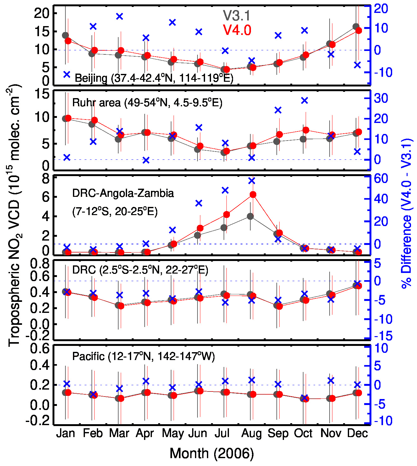
Figure 11Monthly average tropospheric NO2 columns in 2006 calculated from V3.1 (black) and V4.0 (red) data over selected 5∘ latitude × 5∘ longitude boxes from locations that are dominated by either anthropogenic (Beijing, China, and the Ruhr area, Germany), biomass burning (Democratic Republic of Congo – DRC, Angola, and Zambia), lightning (DRC), or no significant (Pacific) NOx sources. The vertical bars show the monthly standard deviation. The blue symbols that correspond to the right y axis show the monthly relative difference (in percent) between V4.0 and V3.1.
In Fig. 12, we examine the monthly variation of tropospheric NO2 columns from the two versions over five highly populated and polluted cities that vary in terrain types ranging from coastal (e.g., Shanghai, Tokyo) to mountainous (e.g., Mexico City). NO2 columns in V4.0 are generally higher than V3.1 by 0 %–30 %, but the difference can occasionally reach up to 50 % in some months. Changes of that order of magnitude in highly polluted areas have implications for the estimation of NOx emissions and trends using these data.

Figure 12Same as Fig. 11, but for a 1∘ latitude × 1∘ longitude box over five highly populated and polluted cities.
In this section, we compare OMI NO2 columns with total column retrievals from ground-based Pandora measurements and integrated tropospheric columns from aircraft spirals at several locations of the DISCOVER-AQ (Deriving Information on Surface Conditions from COlumn and VERtically Resolved Observations Relevant to Air Quality) field campaign held between 2011 and 2014.
3.1 Comparison between OMI and Pandora total column NO2
Here, we compare the total column NO2 retrievals from OMI and the ground-based Pandora spectrometer. Pandora is a compact sun-viewing remote sensing instrument that provides estimates of NO2 column amounts from the surface to the top of the atmosphere (Herman et al., 2009, 2018). The NO2 retrieval approach for Pandora is similar to that of OMI and consists of the DOAS spectral fitting procedure to derive NO2 SCD and its conversion to VCD using AMFs. However, the details differ due to the lack of top-of-atmosphere radiance measurements for the spectral fitting and simplicity in the AMF calculation for Pandora due to its direct-sun measurements.
To compare with the OMI observations, we use Pandora data for sites listed in the Pandonia Global Network (https://www.pandonia-global-network.org/, last access: 10 May 2020). Out of 22 sites, we select 18 sites that we determined to be suitable for comparison. Data from some of the sites (e.g., Rome, Italy) are consistently higher than OMI by over a factor of 2, suggesting that the sites may be in close proximity to local sources that cannot be resolved by OMI. Although some of the selected sites have sporadic and short-term measurements (e.g., Ulsan, South Korea), we consider them for improved sampling and coverage. The collocation criteria include spatial and temporal matching between OMI and Pandora observations by selecting the OMI pixels that encompass the Pandora site and using Pandora 80 s total NO2 column data averaged over ±10 min of OMI observations. We use high-quality data obtained under clear-sky conditions with the root mean square of spectral fitting residuals < 0.05 and NO2 retrieval uncertainty < 0.05 DU (∼ 1.3×10¹⁵ molec. cm−2) for Pandora and with CRF < 0.5 for OMI.
Figure 13 shows a comparison of OMI total NO2 columns (sum of tropospheric and stratospheric columns) to coincidently sampled Pandora direct-sun NO2 column retrievals at a clean site in Izaña on Tenerife, Spain, and a more polluted site in Greenbelt (Maryland, USA). The Izaña Atmospheric Observatory is located on the top of a mountain plateau, with an elevation of 2373 m above sea level. Since the site is free of local anthropogenic influences, Pandora observations likely provide stratospheric and free tropospheric NO2 amounts. In contrast, the Greenbelt site in a suburban Washington DC area has traffic and air quality typical of polluted US cities. As shown in Fig. 13a and b, OMI NO2 retrievals from the two versions are highly consistent (r>0.92), with somewhat higher values in V4.0 compared to V3.1 by 13 % on average in Greenbelt and just 1 % in Izaña. The variations of OMI NO2 from both versions are also broadly consistent with the Pandora measurements. The OMI and Pandora NO2 columns are fairly correlated (r=0.32, N=232) at Izaña and moderately correlated (r=0.51, N=123) at Greenbelt; often the differences between each individual OMI and Pandora observation are significant. Overall, the total column NO2 data from OMI are higher than Pandora, with an average difference of < 16 %. Occasional large discrepancies between OMI and Pandora reflect a combination of spatial heterogeneity, differences in spatial and temporal sampling, differences in the vertical sensitivity of satellite- and ground-based observations, and errors in OMI and Pandora retrievals.
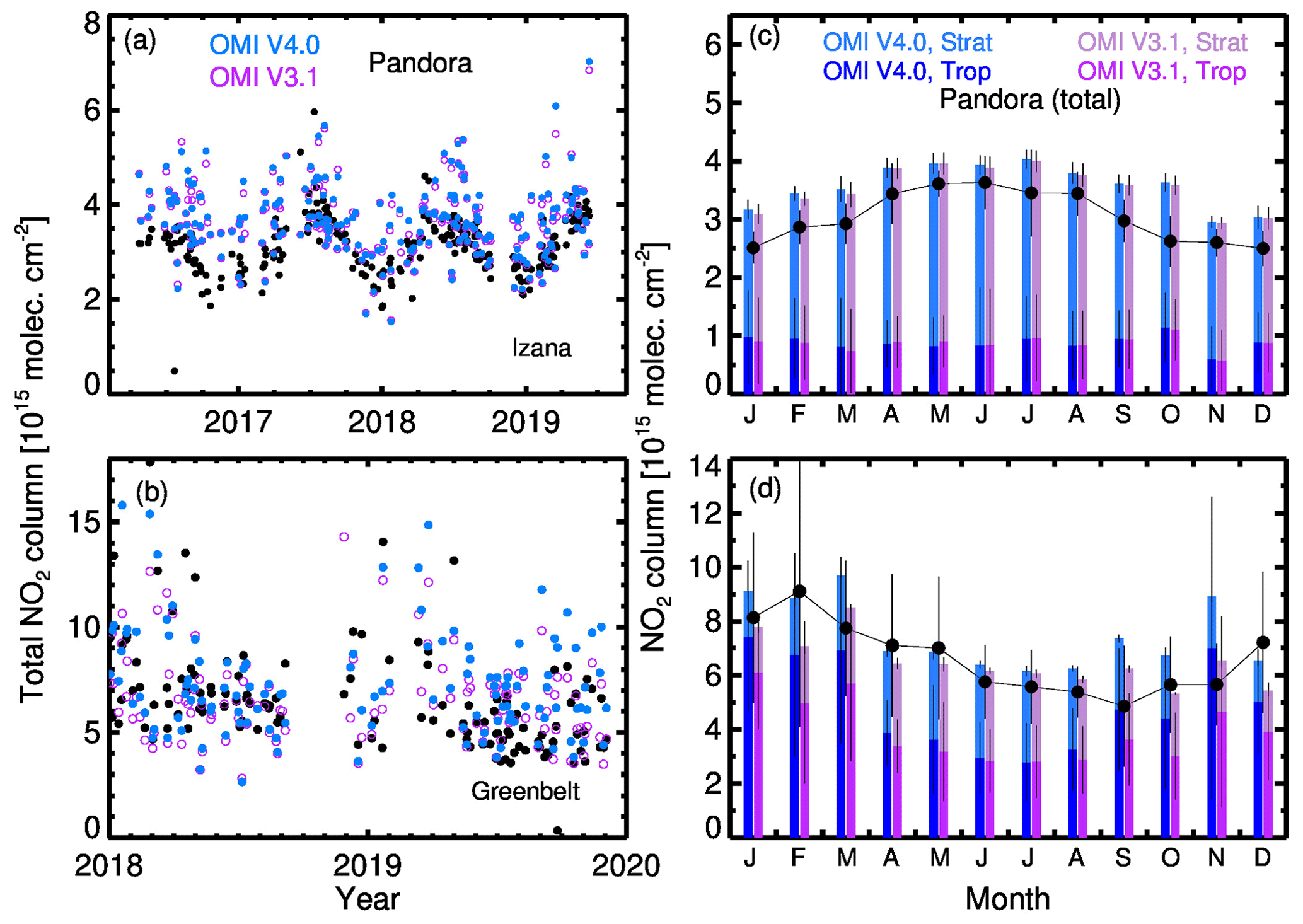
Figure 13The time series of NO2 total columns retrieved from Pandora (black circles) and OMI at (a) Izaña, Spain, and (b) Greenbelt, Maryland, USA, with the OMI retrievals represented by the filled blue (V4.0) and open purple (V3.1) circles. Right panels show the monthly variation of NO2 total columns at (c) Izaña for 2016–2019 and (d) Greenbelt for 2018–2019, as calculated from Pandora (black line with filled circles) and OMI measurements (bars). OMI NO2 total columns retrieved with V4.0 (blue) and V3.1 (purple) are separated into tropospheric and stratospheric components. The vertical lines represent the standard deviation from the average.
Figure 13c and d show the multiyear monthly mean variation of OMI and Pandora NO2 columns. The seasonal variation in Pandora and OMI NO2 columns is highly consistent and exhibits a summer maximum and a fall minimum at Izaña and a winter maximum and summer minimum in Greenbelt. The seasonal variation in the total column reflects that of the stratosphere for Izaña and of the troposphere in Greenbelt. For Izaña, the monthly mean differences between OMI and Pandora range from 8.2 % in June to 38 % in October for V4.0 and from 7.0 % in June to 37 % in October for V3.1. This discrepancy is likely due to the large aerial coverage of OMI pixels including nearby cities, unlike the point measurements made by Pandora at the mountaintop. The average tropospheric NO2 column observed by OMI is 8.9×10¹⁴ molec. cm−2, suggesting significant NO2 amounts in the troposphere with 20 %–32 % contributions to total column NO2 on a monthly scale. For Greenbelt, the monthly mean differences between OMI and Pandora are within ±12 % for the majority of the cases for both versions, with V4.0 improving agreement for February, April, May, and December and worsening somewhat in other months, especially in September and November when the two versions exhibit larger differences in tropospheric NO2 retrievals.
Figure 14 shows average total NO2 columns measured by Pandora and OMI at the 18 selected sites. Although there is a wide range of differences between individual sites, Pandora and OMI observations exhibit a good spatial correlation, with slightly improved correlation for V4.0 (r=0.65, N=1082) compared to V3.1 (r=0.62). The site-specific average values generally agree within ±35 % for columns < 1016 molec. cm−2. For more polluted sites, OMI retrievals tend to be lower than the Pandora data. Although the relationship between Pandora and OMI has not changed appreciably with the updates made in the OMI V4.0 product, the corrections are in the right direction for a majority of the sites. The observed differences should not be interpreted as biases in retrievals but rather as the combined effect of differences in spatial coverage, heterogeneity in the NO2 field, preferential placement of Pandora instruments, and potentially a lack of site-specific profile shapes assumed in OMI retrievals.
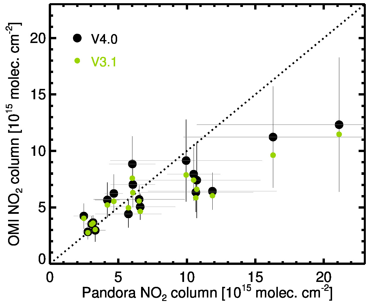
Figure 14The scatter plot of Pandora versus OMI V4.0 (black) and V3.1 (green) average total column NO2 for 18 Pandora sites. The vertical and horizontal lines represent the standard deviations for Pandora and OMI, respectively. The dotted line represents the 1:1 relationship.
3.2 Assessment using DISCOVER-AQ observations
We also use NO2 observations from the DISCOVER-AQ field program to assess OMI NO2 retrievals. The DISCOVER-AQ campaign was composed of four field deployments: the Baltimore–Washington area in Maryland (MD) in July 2011; the San Joaquin Valley in California (CA) in January–February 2013; Houston, Texas (TX), in September 2013; and Denver, Colorado (CO), in July–August 2014. An observing strategy of the campaign was to carry out systematic and concurrent in situ and remote sensing observations from a network of ground sites and research aircraft that spiraled over each site two to four times a day. The payload of the P-3B research aircraft included in situ measuring instruments to measure NO2 profiles in the 0.3–5 km altitude range. Each campaign hosted ground-based networks of surface monitors to provide in situ NO2 observations and Pandora spectrometers to measure NO2 column amounts.
We use Pandora NO2 column observations and in situ NO2 spiral data spatially and temporally matched to OMI on clear and partially cloudy (cloud radiance fraction < 0.5) days. Airborne measurements were carried out using the four-channel chemiluminescence instrument from the National Center for Atmospheric Research (Ridley and Grahek, 1990) and the thermal dissociation laser-induced fluorescence instrument from the University of Berkeley (Thornton et al., 2000). Despite differences in the measurement technique and sampling strategy, NO2 measurements from the two instruments are highly consistent and generally agree within 10 %, with the exception of ∼ 32 % difference for Houston (Choi et al., 2020). Here, we use the 1 s merged data from the chemiluminescence instrument only, taking advantage of its high-frequency measurements. The spiral data are extended to the ground by using coincident in situ surface NO2 measurements sampled over the duration of spiral (∼ 20 min). To account for NO2 amounts in the missing portion from the highest aircraft altitude to the tropopause, we use NO2 from the GMI simulation. Like the surface data, the Pandora total column NO2 data are averaged over the duration of each aircraft spiral. For OMI, we include data from all cross-track positions that are not subject to the row anomaly.
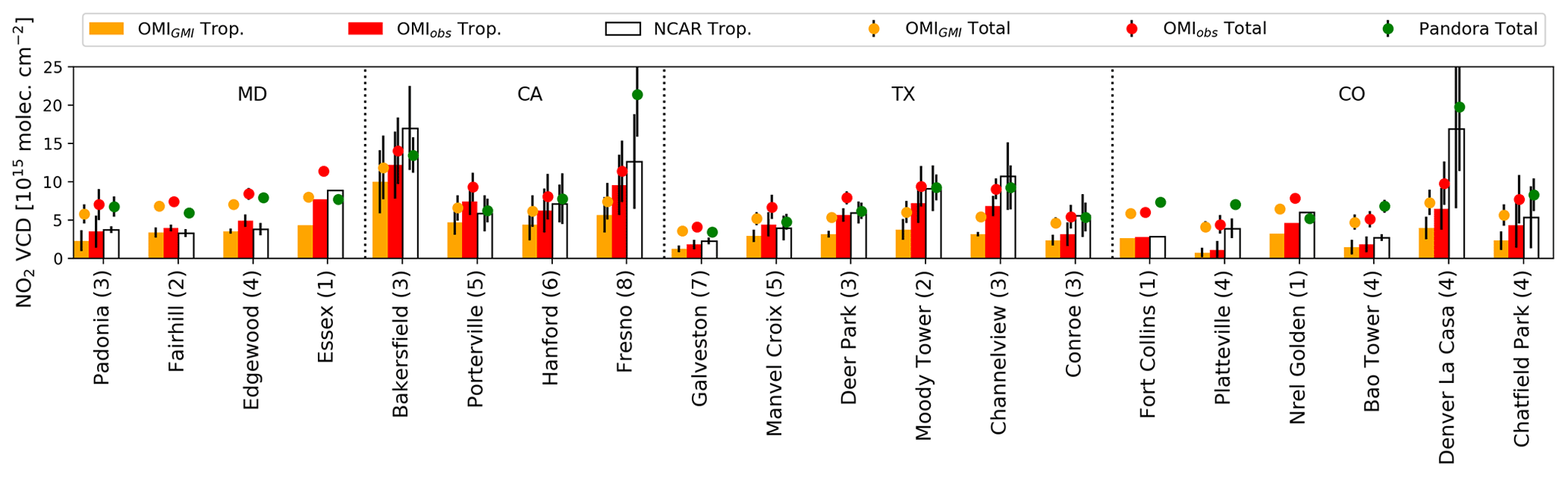
Figure 15Site average total (circles) and tropospheric (bars) NO2 column data from the P-3B spiral (white bars), Pandora (green circles), and OMI (orange and red). The OMI tropospheric columns are derived using GMI-simulated (OMIGMI, orange) and P-3B (OMIobs, red) NO2 profiles. The vertical bars for sites with over two observations represent the standard deviations.
Figure 15 and Table 2 show a summary of the comparison of OMI V4.0 and V3.1 NO2 columns to vertically integrated tropospheric columns from the P-3B aircraft at 20 spiral locations. Overall, tropospheric NO2 columns from OMI and aircraft spirals suggest poor agreement but a good correlation (r=0.74, N=100), with slightly improved agreement for V4.0 compared to V3.1. The agreement and correlations between OMI and P-3B observations vary by campaign locations (e.g., r=0.4 for MD to r=0.81 for CA for V4.0). The level of improvements from V3.1 to V4.0 also varies from 1.2 % in TX to 9.8 % in CA. OMI retrievals are usually lower than the aircraft data, with larger differences for sites with larger NO2 gradients and columns (e.g., Denver–LaCasa, CO; Fresno, CA). OMI is rarely higher than the aircraft data as this usually happens over relatively cleaner sites (e.g., Fairhill, MD). This alternating nature of the variation in results in polluted versus clean areas suggests that OMI's large footprint size and the narrow spiral radius (∼ 4 km) of the aircraft are likely the primary causes of the observed differences. This was demonstrated in Choi et al. (2020) by using high-resolution Community Multi-scale Air Quality Model (CMAQ) simulations. Additional contributions to the observed differences could come from OMI retrieval errors arising from the use of coarse-resolution GMI-based a priori NO2 profile shapes in the AMF calculation. Such profile-related retrieval errors can be partially accounted for by replacing GMI profiles with the aircraft-observed NO2 profiles (OMIobs). The use of observed profiles in the OMI retrievals from both versions leads to a slight change in correlation but a 20 %–35 % reduction in the mean difference between OMI and aircraft observations, highlighting the role of a priori profiles in NO2 retrievals as suggested by previous studies (Russell et al., 2011; Lamsal et al., 2014; Goldberg et al., 2017; Laughner et al., 2019; Choi et al., 2020). The campaign average difference between OMI and aircraft observations is −38.8 % in V3.1 and −23.1 % in V4.0, resulting in a net improvement of 15.7 % with V4.0. We note here that the aircraft-observed profiles can be very different from the actual profiles over OMI's FOVs (pixels) due to a difference in the sampling domains for the two measurements.
Table 2Comparison of OMI V3.1 and V4.0 NO2 retrievals based on a priori NO2 profiles from GMI (OMI) and P-3B aircraft observations (OMIobs) to P-3B observations during the DISCOVER-AQ field campaign. Shown here are the correlation coefficient (r) and mean difference, which is calculated as OMI minus validation data.
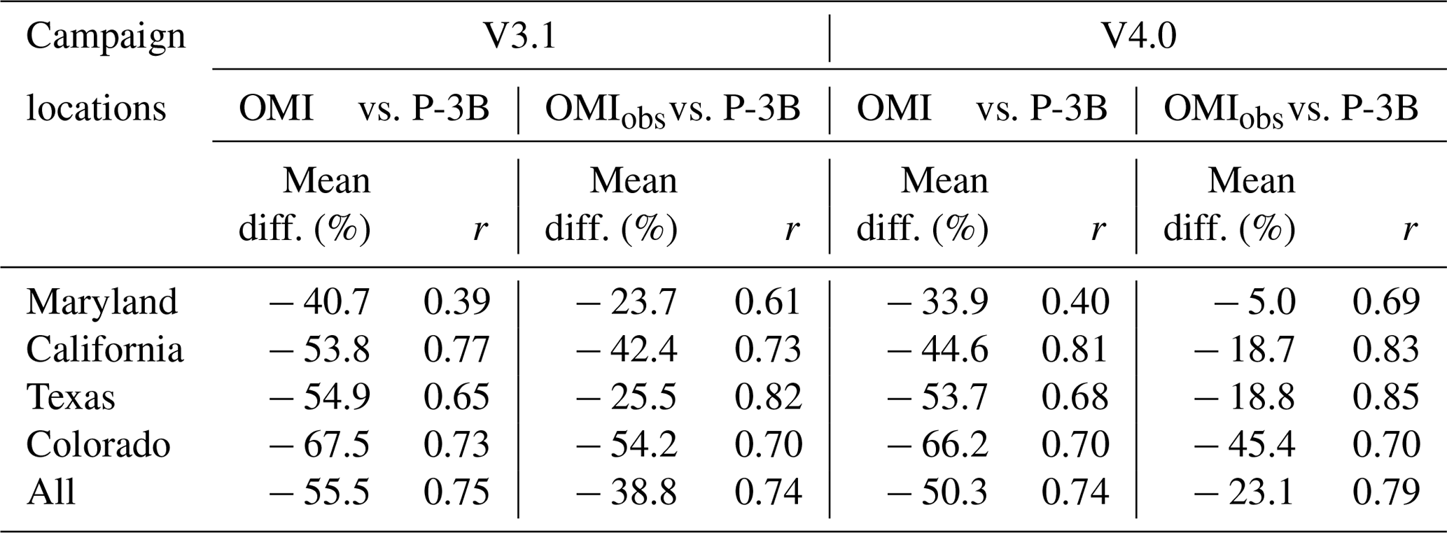
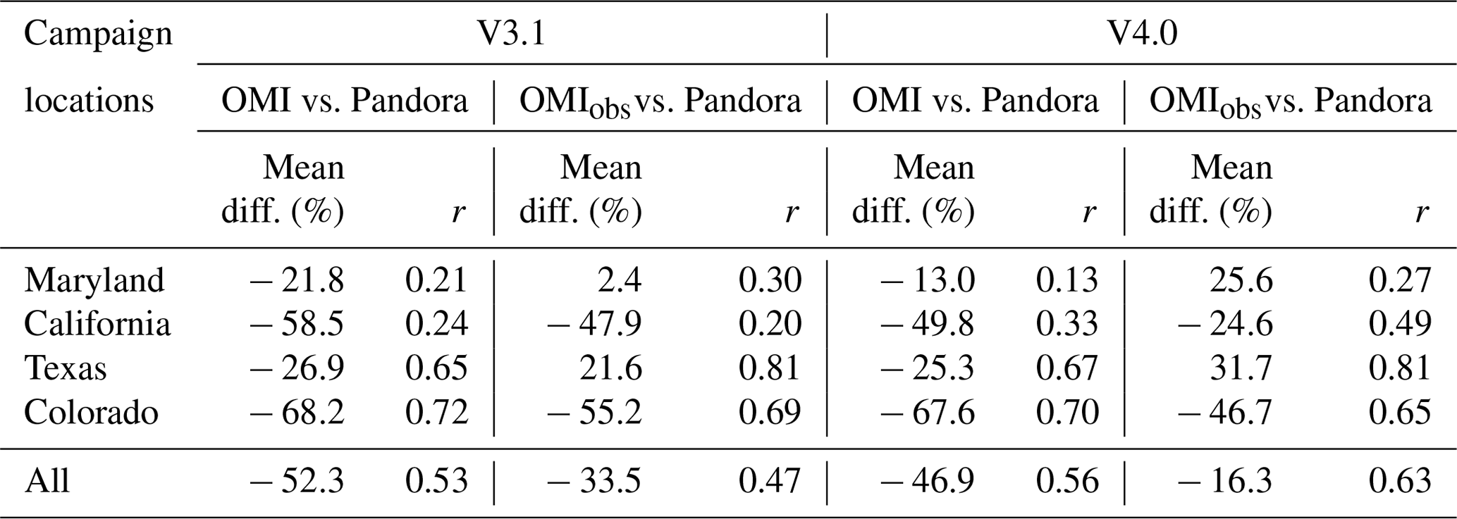
Figure 15 and Table 3 also show the comparison between the OMI and Pandora total column retrievals at the 20 DISCOVER-AQ sites. The correlations between collocated OMI V4.0 and Pandora observations for individual campaign locations vary from fair (r=0.13 for MD) to good (r=0.70 for CO), with a moderate correlation (r=0.56, N=83) for all observations from the four locations. The changes in correlation from V3.1 to V4.0 are generally small, with a minor improvement in CA and deterioration in MD. Compared to the aircraft observations, the OMI data generally show better agreement with the Pandora retrievals, with the smallest difference in MD and the largest difference in CO. Compared to V3.1, the agreement is improved for V4.0 by up to 9 %. The use of aircraft-observed NO2 profiles in AMF calculations leads to higher OMI column retrievals than those from Pandora for MD and TX and lower columns than Pandora for CA and CO. Overall, total column retrievals from OMI V3.1 and V4.0 are respectively 33.5 % and 16.3 % lower than Pandora; this change is consistent with the comparison between OMI and P-3B observations. The observed discrepancy between the OMI, aircraft spiral, and Pandora data points to general difficulties in comparing observations of different spatial resolutions for a short-lived trace gas like NO2 that has large spatial gradients, especially in the boundary layer.
Table 3Same as Table 2, but with Pandora NO2 column observations.
We have described a series of significant improvements made to the operational OMI NO2 standard product (OMNO2) algorithm. The new version, version 4.0 (V4.0), of the OMNO2 product, recently released to the public at the NASA Goddard Earth Sciences Data and Information Services Center (GES DISC), mainly relies on improved methods and high-resolution inputs for a more accurate determination of air mass factors (AMFs). Major improvements include the following: (1) a new O2–O2 cloud algorithm to estimate cloud radiance fraction (CRF) and cloud optical centroid pressure (OCP), both required for the AMF calculation; (2) new MODIS BRDF-derived geometry-dependent surface Lambertian equivalent reflectivity (GLER) input data used in both the NO2 and cloud retrievals; (3) improved terrain pressure calculated for OMI's footprint; and (4) improved surface and cloud treatments over snow and ice surfaces. Over open-water areas, inputs to the GLER calculations include chlorophyll concentrations from MODIS, wind speed data from the Advanced Microwave Scanning Radiometer–Earth Observing System (AMSR-E) and the Special Microwave Imager–Sounder (SSMIS) instruments, and wind direction data from the NASA GEOS-5 model. The following algorithmic steps remain unchanged: the scheme for separating stratospheric and tropospheric components, first implemented in version 2.1 (Bucsela et al., 2013; Lamsal et al., 2014); an optimized spectral fitting algorithm used for NO2 slant column density retrievals (Marchenko et al., 2015); and the use of annually varying monthly mean inputs derived from the Global Modeling Initiative (GMI) (e.g., NO2 vertical profile shapes), as implemented in version 3.0 (Krotkov et al., 2017).
The changes in inputs result in substantial changes in tropospheric AMFs (and thus VCDs) in V4.0 relative to the previous version (V3.1). The geometry-dependent GLER data computed for OMI observations used in V4.0 differ considerably from the OMI-derived climatological LER data (Kleipool et al., 2008) used in V3.1. The data from GLER (a unitless value with 0.0–1.0 range) are generally lower, by < 0.05, than the climatological LER data over land and ocean outside sun-glint areas; GLER is much higher over sun-glint areas and reaches more than 0.3 due to the geometry-dependent Fresnel reflection. The cloud parameters (OCP and CRF) retrieved from the new O2–O2 cloud algorithm described here and those from the operational cloud algorithm (Veefkind et al., 2016) used in V3.1 exhibit significant differences, with generally larger values for both parameters in V4.0 compared to V3.1 but noticeable exceptions over sun-glint areas where CRFs in V4.0 are lower than V3.1 by < 0.3. Over snow and ice surfaces, identified by near-real-time ice and snow extent (NISE) flags in the OMI L1b data, various adjustments are made in V4.0 for GLER, OCP, and CRF by using other diagnostic parameters (e.g., scene pressure) retrieved by the new cloud algorithm. The scattering weights and tropospheric AMFs for NO2 respond to the changes in these input parameters in a complicated way. Typically, tropospheric AMFs decrease with the use of GLER and increase with the use of the new cloud parameters, with exceptions over water surfaces affected by sun glint, for which we observe the opposite effect. Over highly polluted areas, the effect from GLER is augmented by the effect from the new cloud parameters, resulting in a considerable decrease in the tropospheric AMF. Changes in tropospheric AMFs resulting from updates in the treatment of snow- and ice-covered areas are also significant. Changes in the adopted terrain pressure (V4.0 vs. V3.1) can also have a sizable effect on tropospheric AMFs, particularly over areas with a complex terrain. In contrast, for stratospheric AMFs the combined impact of all of these algorithmic updates is negligible.
The changes in tropospheric AMFs translate directly into changes in tropospheric NO2 retrievals and indirectly into stratospheric NO2 estimates. Over background and low-column NO2 areas, tropospheric NO2 column estimates have not changed appreciably from V3.1 to V4.0. Over more polluted areas, the tropospheric NO2 retrievals have typically increased by 10 %–40 % from V3.1 to V4.0, mostly in direct proportion to the pollution level. Most of the increase in highly polluted areas is driven by the change in the surface reflectivity data used in the AMF calculation, with additional increases due to changes in the cloud parameters. Changes in the stratospheric NO2 estimates are usually within ±2.5 %, which is close to the range of estimated uncertainties of stratospheric NO2 estimates.
A global assessment of V4.0 tropospheric and stratospheric NO2 products was performed by a thorough evaluation of their consistency with the data from V3.1, which was carefully evaluated in our previous works (e.g., Krotkov et al., 2017; Choi et al., 2020). In addition, we use NO2 measurements made by independent ground- and aircraft-based instruments to evaluate the V4.0 product. The comparison of OMI total column NO2 data to collocated Pandora observations at its 18 global network and 20 DISCOVER-AQ locations suggests that OMI and Pandora are generally highly consistent, exhibit similar seasonal variation, and agree within their expected uncertainties of 2.7×10¹⁵ molec. cm−2 for Pandora (Herman et al., 2009) and ∼ 30 % for OMI under clear-sky conditions (Boersma et al., 2011; Bucsela et al., 2013). Individual data points differ considerably, and OMI tends to be lower than Pandora over highly polluted areas with spatially inhomogeneous NO2. The comparison of OMI tropospheric NO2 column retrievals to columns derived from the aircraft spirals and surface data during the DISCOVER-AQ campaign also suggests general agreement in spatial variation, but OMI values are about a factor of 2 lower in polluted environments. This difference is partly due to inaccurate a priori assumptions but primarily to OMI's relatively large pixels. The use of observed NO2 profiles as a priori information reduces the bias from ∼ 50 % to 23 % on average. A multi-axis differential optical absorption spectrometer (MAX-DOAS) (e.g., Chan et al., 2019) or high-spatial-resolution measurements from aircraft (e.g., Nowlan et al., 2016; Lamsal et al., 2017; Judd et al., 2019) would provide a more comprehensive validation by mapping the NO2 distributions over the complete areas of aircraft spirals and the satellite FOVs.
In this study, we focused on improving the surface and cloud parameters in the NASA standard NO2 product retrievals. To further improve the retrieval accuracy, it is important to incorporate improved retrieval methods and auxiliary information, such as high-resolution a priori NO2 profiles. For instance, current cloud algorithms based on the MLER model treat aerosols implicitly by providing effective (cloud + aerosol) CRF and effective cloud OCP, both necessary inputs for AMF calculations. Cloud effects on trace gas retrievals can be compromised by unknown aerosol effects, which lead to errors in AMF calculations. Therefore, the use of the GLER product in the NO2 algorithm will greatly benefit from an explicit accounting for aerosol effects, particularly over polluted regions. We have recently developed an explicit and consistent aerosol correction method that can be applied consistently in both cloud and NO2 retrievals (Vasilkov et al., 2020); it uses a model of aerosol optical properties from a global aerosol assimilation system paired with radiative transfer calculations. This approach allows us to account for aerosols within the OMI cloud and NO2 algorithms with relatively small changes and will be used in the next version of the NO2 algorithm.
The Level-2 swath-type column NO2 product (OMNO2; https://doi.org/10.5067/Aura/OMI/DATA2017; Krotkov et al., 2019a) is available from the NASA Goddard Earth Sciences Data and Information Services Center (GES DISC) website (https://doi.org/10.5067/Aura/OMI/DATA2018, Krotkov et al., 2019b). Other OMNO2-associated NO2 products, such as the Level-2 gridded column product, OMNO2G, and the Level-3 gridded column product, OMNO2d, both sampled at regular 0.25∘ latitude × 0.25∘ longitude grids, are distributed through the NASA GES DISC (https://doi.org/10.5067/Aura/OMI/DATA3007, Krotkov et al., 2019c) and GIOVANNI (https://giovanni.gsfc.nasa.gov/giovanni/, NASA, 2020a) websites. An additional high-spatial-resolution (0.1∘ × 0.1∘ latitude–longitude grid) OMNO2d product (OMNO2d_HR) is also made available through the NASA AVDC website (https://avdc.gsfc.nasa.gov/pub/data/satellite/Aura/OMI/V03/L3/OMNO2d_HR/, NASA, 2020b). The AVDC website also hosts overpass files for several hundred sites around the globe (https://avdc.gsfc.nasa.gov/pub/data/satellite/Aura/OMI/V03/L2OVP/OMNO2/, NASA, 2020c).
LNL, NAK, JJ, and AV designed the data analysis. WQ, ZF, NAK, DH, and AV developed and evaluated the GLER product. EY, SM, AV, NAK, JJ, and BF developed and evaluated the cloud product. LNL, NAK, SM, WHS, and EB have developed and evaluated the NASA NO2 standard product. LNL and SC conducted validation of the OMI NO2 products using Pandora and other independent observations. LNL, AV, SM, and ZF wrote the paper with comments from all coauthors.
The authors declare that they have no conflict of interest.
We acknowledge the NASA Earth Science Division for funding OMI NO2 product development and analysis. The Dutch–Finnish-built OMI is part of the NASA EOS Aura satellite payload. KNMI and the Netherlands Space Agency (NSO) manage the OMI project. We acknowledge the NASA Pandora, ESA Pandonia, and NASA DISCOVER-AQ projects for free access to the data. We thank the two anonymous reviewers for their helpful comments.
This research has been supported by the NASA Earth Science Division (grant no. 80NSSC18M0086 for partial support).
This paper was edited by Dominik Brunner and reviewed by two anonymous referees.
Beirle, S., Boersma, K. F., Platt, U., Lawrence, M. G., and Wagner, T.: Megacity emissions and lifetimes of nitrogen oxides probed from space, Science, 333, 1737–1739, https://doi.org/10.1126/science.1207824, 2011.
Boersma, K. F., Eskes, H. J., Dirksen, R. J., van der A, R. J., Veefkind, J. P., Stammes, P., Huijnen, V., Kleipool, Q. L., Sneep, M., Claas, J., Leitão, J., Richter, A., Zhou, Y., and Brunner, D.: An improved tropospheric NO2 column retrieval algorithm for the Ozone Monitoring Instrument, Atmos. Meas. Tech., 4, 1905–1928, https://doi.org/10.5194/amt-4-1905-2011, 2011.
Boersma, K. F., Eskes, H. J., Richter, A., De Smedt, I., Lorente, A., Beirle, S., van Geffen, J. H. G. M., Zara, M., Peters, E., Van Roozendael, M., Wagner, T., Maasakkers, J. D., van der A, R. J., Nightingale, J., De Rudder, A., Irie, H., Pinardi, G., Lambert, J.-C., and Compernolle, S. C.: Improving algorithms and uncertainty estimates for satellite NO2 retrievals: results from the quality assurance for the essential climate variables (QA4ECV) project, Atmos. Meas. Tech., 11, 6651–6678, https://doi.org/10.5194/amt-11-6651-2018, 2018.
Bucsela, E. J., Celarier, E. A., Wenig, M. O., Gleason, J. F., Veefkind, J. P., Boersma, K. F., and Brinksma, E. J.: Algorithm for NO2 vertical column retrieval from the Ozone Monitoring Instrument, IEEE Trans. Geosci. Remote Sens., 44, 1245–1258, 2006.
Bucsela, E. J., Krotkov, N. A., Celarier, E. A., Lamsal, L. N., Swartz, W. H., Bhartia, P. K., Boersma, K. F., Veefkind, J. P., Gleason, J. F., and Pickering, K. E.: A new stratospheric and tropospheric NO2 retrieval algorithm for nadir-viewing satellite instruments: applications to OMI, Atmos. Meas. Tech., 6, 2607–2626, https://doi.org/10.5194/amt-6-2607-2013, 2013.
Cai, K., Li, S., Zheng, F., Yu, C., Zhang, X., Liu, Y., and Li, Y.: Spatio-temporal Variations in NO2 and PM2.5 over the Central Plains Economic Region of China during 2005–2015 Based on Satellite Observations, Aer. Air Qual. Res., 5, 1221–1235, https://doi.org/10.4209/aaqr.2017.10.0394, 2018.
Canty, T. P., Hembeck, L., Vinciguerra, T. P., Anderson, D. C., Goldberg, D. L., Carpenter, S. F., Allen, D. J., Loughner, C. P., Salawitch, R. J., and Dickerson, R. R.: Ozone and NOx chemistry in the eastern US: evaluation of CMAQ/CB05 with satellite (OMI) data, Atmos. Chem. Phys., 15, 10965–10982, https://doi.org/10.5194/acp-15-10965-2015, 2015.
Castellanos, P., and Boersma, K. F.: Reductions in nitrogen oxides over Europe driven by environmental policy and economic recession, Sci. Rep., 2, 265, https://doi.org/10.1038/srep00265, 2012.
Celarier, E. A., Brinksma, E. J., Gleason, J. F., Veefkind, J. P., Cede, A., Herman, J. R., Ionov, D., Goutail, F., Pommereau, J.-P., Lambert, J.‐C., van Roozendael, M., Pinardi, G., Wittrock, F., Schönhardt, A., Richter, A., Ibrahim, O. W., Wagner, T., Bojkov, B., Mount, G., Spinei, E., Chen, C. M., Pongetti, T. J., Sander, S. P., Bucsela, E. J., Wenig, M. O., Swart, D. P. J., Volten, H., Kroon, M., and Levelt, P. F.: Validation of Ozone Monitoring Instrument nitrogen dioxide columns, J. Geophys. Res., 113, D15S15, https://doi.org/10.1029/2007JD008908, 2008.
Chance, K., Kurosu, T.P., and Sioris, K. E.: Undersampling correction for array detector-based satellite spectrometers, Appl. Opt., 44, 1296–1304, 2005.
Chan, K. L., Wang, Z., Ding, A., Heue, K.-P., Shen, Y., Wang, J., Zhang, F., Shi, Y., Hao, N., and Wenig, M.: MAX-DOAS measurements of tropospheric NO2 and HCHO in Nanjing and a comparison to ozone monitoring instrument observations, Atmos. Chem. Phys., 19, 10051–10071, https://doi.org/10.5194/acp-19-10051-2019, 2019.
Choi, S., Lamsal, L. N., Follette-Cook, M., Joiner, J., Krotkov, N. A., Swartz, W. H., Pickering, K. E., Loughner, C. P., Appel, W., Pfister, G., Saide, P. E., Cohen, R. C., Weinheimer, A. J., and Herman, J. R.: Assessment of NO2 observations during DISCOVER-AQ and KORUS-AQ field campaigns, Atmos. Meas. Tech., 13, 2523–2546, https://doi.org/10.5194/amt-13-2523-2020, 2020.
Cooper, M. J., Martin, R. V., Lyapustin, A. I., and McLinden, C. A.: Assessing snow extent data sets over North America to inform and improve trace gas retrievals from solar backscatter, Atmos. Meas. Tech., 11, 2983–2994, https://doi.org/10.5194/amt-11-2983-2018, 2018.
Cox, C. and Munk, W.: Statistics of the sea surface derived from sun glitter, J. Mar. Res., 13, 198–227, 1954.
Dave, J. V.: Effect of aerosol on the estimation of total ozone in an atmospheric column from the measurements of the ultraviolet radiance, J. Atmos. Sci., 35, 899–911, 1978.
de Foy, B., Lu, Z., Streets, D. G., Lamsal, L. N., and Duncan, B. N.: Estimates of power plant NOx emissions and lifetimes from OMI NO2 satellite retrievals, Atmos. Environ., 116, 1–11, https://doi.org/10.1016/j.atmosenv.2015.05.056, 2015.
Dirksen, R., Dobber, M., Voors, R., and Levelt, P.: Prelaunch characterization of the Ozone Monitoring Instrument transfer function in the spectral domain, Appl. Opt., 45, 3972–3981, 2006.
Dix, B., Bruin, J., Roosenbrand, E., Vlemmix, T., Francoeur, C., Gorchov-Negron, A., McDonald, B., Zhizhin, M., Elvidge, C., Veefkind, P., Levelt, P., and de Gouw, J.: Nitrogen Oxide Emissions from U.S. Oil and Gas Production: Recent Trends and Source Attribution, Geophys. Res. Lett., 1, e2019GL085866, https://doi.org/10.1029/2019gl085866, 2020.
Dobber, M., Kleipool, Q., Dirksen, R., Levelt, P., Jaross, G., Taylor, S., Kelly, T., Flynn, L., Leppelmeier, G., and Rozemeijer, N.: Validation of Ozone Monitoring Instrument level 1b data products, J. Geophys. Res., 113, D15S06, https://doi.org/10.1029/2007JD008665, 2008.
Douglass, A. R., Stolarski, R. S., Strahan, S. E., and Connell, P. S.: Radicals and reservoirs in the GMI chemistry and transport model: Comparison to measurements, J. Geophys. Res., 109, D16302, https://doi.org/10.1029/2004JD004632, 2004.
Duncan, B. N., Yoshida, Y., Foy, B., Lamsal, L. N., Streets, D. G., Lu, Z., Pickering, K. E., and Krotkov, N. A.: The observed response of Ozone Monitoring Instrument (OMI) NO2 columns to NOx emission controls on power plants in the United States: 2005–2011, Atmos. Environ., 102–111, https://doi.org/10.1016/j.atmosenv.2013.08.068, 2013.
Duncan, B. N., Lamsal, L. N., Thompson, A. M., Yoshida, Y., Lu, Z., Streets, D. G., Hurwitz, M. M., Pickering, K. E.: A space-based, high-resolution view of notable changes in urban NOx pollution around the world (2005–2014), J. Geophys. Res., 121, 976–996, https://doi.org/10.1002/2015JD024121, 2016.
Eskes, H. J. and Boersma, K. F.: Averaging kernels for DOAS total-column satellite retrievals, Atmos. Chem. Phys., 3, 1285–1291, https://doi.org/10.5194/acp-3-1285-2003, 2003.
Fasnacht, Z., Vasilkov, A., Haffner, D., Qin, W., Joiner, J., Krotkov, N., Sayer, A. M., and Spurr, R.: A geometry-dependent surface Lambertian-equivalent reflectivity product for UV–Vis retrievals – Part 2: Evaluation over open ocean, Atmos. Meas. Tech., 12, 6749–6769, https://doi.org/10.5194/amt-12-6749-2019, 2019.
Geddes, J. A. and Martin, R. V.: Global deposition of total reactive nitrogen oxides from 1996 to 2014 constrained with satellite observations of NO2 columns, Atmos. Chem. Phys., 17, 10071–10091, https://doi.org/10.5194/acp-17-10071-2017, 2017.
Gelaro, R., McCarty, W., Suárez, M. J., Todling, R., Molod, A., Takacs, L., Randles, C. A., Darmenov, A., Bosilovich, M. G., Reichle, R., Wargan, K., Coy, L., Cullather, R., Draper, C., Akella, S., Buchard, V., Conaty, A., da Silva, A. M., Gu, W., Kim, G., Koster, R., Lucchesi, R., Merkova, D., Nielsen, J. E., Partyka, G., Pawson, S., Putman, W., Rienecker, M., Schubert, S. D., Sienkiewicz, M., and Zhao, B.: The Modern-Era Retrospective Analysis for Research and Applications, Version 2 (MERRA-2), J. Climate, 30, 5419–5454, https://doi.org/10.1175/JCLI-D-16-0758.1, 2017.
Ghude, S. D., Kulkarni, S. H., Jena, C., Pfister, G. G., Beig, G., Fadnavis, S., and van der A, R. J.: Application of satellite observations for identifying regions of dominant sources of nitrogen oxides over the Indian Subcontinent, J. Geophys. Res., 2, 1075–1089, https://doi.org/10.1029/2012jd017811, 2013.
Goldberg, D. L., Lamsal, L. N., Loughner, C. P., Swartz, W. H., Lu, Z., and Streets, D. G.: A high-resolution and observationally constrained OMI NO2 satellite retrieval, Atmos. Chem. Phys., 17, 11403–11421, https://doi.org/10.5194/acp-17-11403-2017, 2017.
Goldberg, D. L., Saide, P. E., Lamsal, L. N., de Foy, B., Lu, Z., Woo, J.-H., Kim, Y., Kim, J., Gao, M., Carmichael, G., and Streets, D. G.: A top-down assessment using OMI NO2 suggests an underestimate in the NOx emissions inventory in Seoul, South Korea, during KORUS-AQ, Atmos. Chem. Phys., 19, 1801–1818, https://doi.org/10.5194/acp-19-1801-2019, 2019a.
Goldberg, D., Lu, Z., Oda, T., Lamsal, L. N, Liu, F., Griffin, D., McLinden, C., Krotkov, N. A., Duncan, B. N., and Streets, D.: Exploiting OMI NO2 satellite observations to infer fossil-fuel CO2 emissions from U.S. megacities, Sci. Total Environ., 695, 133805, https://doi.org/10.1016/j.scitotenv.2019.133805, 2019b.
Gu, J., Chen, L., Yu, C., Li, S., Tao, J., Fan, M., Xiong, X., Wang, Z., Shang, H., and Su, L.: Ground-Level NO2 Concentrations over China Inferred from the Satellite OMI and CMAQ Model Simulations, Remote Sens., 6, 519, https://doi.org/10.3390/rs9060519, 2017.
Han, K., Lee, C., Lee, J., Kim, J., and Song, C.: A comparison study between model-predicted and OMI-retrieved tropospheric NO2 columns over the Korean peninsula, Atmos. Environ., 17, 2962–2971, https://doi.org/10.1016/j.atmosenv.2010.10.016, 2011.
Herman, J., Cede, A., Spinei, E., Mount, G., Tzortziou, M., and Abuhassan, N.: NO2 column amounts from ground-based Pandora and MFDOAS spectrometers using the direct-sun DOAS technique: Intercomparisons and application to OMI validation, J. Geophys. Res.-Atmos., 114, D13307, https://doi.org/10.1029/2009JD011848, 2009.
Herman, J., Spinei, E., Fried, A., Kim, J., Kim, J., Kim, W., Cede, A., Abuhassan, N., and Segal-Rozenhaimer, M.: NO2 and HCHO measurements in Korea from 2012 to 2016 from Pandora spectrometer instruments compared with OMI retrievals and with aircraft measurements during the KORUS-AQ campaign, Atmos. Meas. Tech., 11, 4583–4603, https://doi.org/10.5194/amt-11-4583-2018, 2018.
Herron-Thorpe, F. L., Lamb, B. K., Mount, G. H., and Vaughan, J. K.: Evaluation of a regional air quality forecast model for tropospheric NO2 columns using the OMI/Aura satellite tropospheric NO2 product, Atmos. Chem. Phys., 10, 8839–8854, https://doi.org/10.5194/acp-10-8839-2010, 2010.
Hudman, R. C., Moore, N. E., Mebust, A. K., Martin, R. V., Russell, A. R., Valin, L. C., and Cohen, R. C.: Steps towards a mechanistic model of global soil nitric oxide emissions: implementation and space based-constraints, Atmos. Chem. Phys., 12, 7779–7795, https://doi.org/10.5194/acp-12-7779-2012, 2012.
Ialongo, I., Herman, J., Krotkov, N., Lamsal, L., Boersma, K. F., Hovila, J., and Tamminen, J.: Comparison of OMI NO2 observations and their seasonal and weekly cycles with ground-based measurements in Helsinki, Atmos. Meas. Tech., 9, 5203–5212, https://doi.org/10.5194/amt-9-5203-2016, 2016.
Joiner, J., Bhartia, P., Cebula, R., Hilsenrath, E., McPeters, R., and Park, H.: Rotational Raman scattering (Ring effect) in satellite backscatter ultraviolet measurements, Appl. Opt., 34, 4513–4525, 1995.
Joiner J. and Vasilkov, A. P.: First Results from the OMI Rotational-Raman Scattering Cloud Pressure Algorithm, IEEE Trans. Geophys. Remote Sens., 44, 1272–1282, 2006.
Joiner, J., Vasilkov, A. P., Gupta, P., Bhartia, P. K., Veefkind, P., Sneep, M., de Haan, J., Polonsky, I., and Spurr, R.: Fast simulators for satellite cloud optical centroid pressure retrievals; evaluation of OMI cloud retrievals, Atmos. Meas. Tech., 5, 529–545, https://doi.org/10.5194/amt-5-529-2012, 2012.
Judd, L. M., Al-Saadi, J. A., Janz, S. J., Kowalewski, M. G., Pierce, R. B., Szykman, J. J., Valin, L. C., Swap, R., Cede, A., Mueller, M., Tiefengraber, M., Abuhassan, N., and Williams, D.: Evaluating the impact of spatial resolution on tropospheric NO2 column comparisons within urban areas using high-resolution airborne data, Atmos. Meas. Tech., 12, 6091–6111, https://doi.org/10.5194/amt-12-6091-2019, 2019.
Kim, H. C., Lee, P., Judd, L., Pan, L., and Lefer, B.: OMI NO2 column densities over North American urban cities: the effect of satellite footprint resolution, Geosci. Model Dev., 9, 1111–1123, https://doi.org/10.5194/gmd-9-1111-2016, 2016.
Kleipool, Q. L., Dobber, M. R., de Haan, J. F., and Levelt, P. F.: Earth surface reflectance climatology from 3 years of OMI data, J. Geophys. Res., 113, D18308, https://doi.org/10.1029/2008JD010290, 2008.
Koelemeijer, R. B. A., Stammes, P., Hovenier, J. W., and de Haan, J. F.: A fast method for retrieval of cloud parameters using oxygen A-band measurements from the Global Ozone Monitoring Experiment, J. Geophys. Res., 106, 3475–3496, 2001.
Konovalov, I. B., Berezin, E. V., Ciais, P., Broquet, G., Zhuravlev, R. V., and Janssens-Maenhout, G.: Estimation of fossil-fuel CO2 emissions using satellite measurements of “proxy” species, Atmos. Chem. Phys., 16, 13509–13540, https://doi.org/10.5194/acp-16-13509-2016, 2016.
Krotkov, N. A., McLinden, C. A., Li, C., Lamsal, L. N., Celarier, E. A., Marchenko, S. V., Swartz, W. H., Bucsela, E. J., Joiner, J., Duncan, B. N., Boersma, K. F., Veefkind, J. P., Levelt, P. F., Fioletov, V. E., Dickerson, R. R., He, H., Lu, Z., and Streets, D. G.: Aura OMI observations of regional SO2 and NO2 pollution changes from 2005 to 2015, Atmos. Chem. Phys., 16, 4605–4629, https://doi.org/10.5194/acp-16-4605-2016, 2016.
Krotkov, N. A., Lamsal, L. N., Celarier, E. A., Swartz, W. H., Marchenko, S. V., Bucsela, E. J., Chan, K. L., Wenig, M., and Zara, M.: The version 3 OMI NO2 standard product, Atmos. Meas. Tech., 10, 3133–3149, https://doi.org/10.5194/amt-10-3133-2017, 2017.
Krotkov, N. A., Lamsal, L. N., Marchenko, S. V., Bucsela, E. J., Swartz, W. H., Joiner, J., and the OMI core team: OMI/Aura Nitrogen Dioxide (NO2) Total and Tropospheric Column 1-orbit L2 Swath 13×24 km V003, Greenbelt, MD, USA, Goddard Earth Sciences Data and Information Services Center (GES DISC), https://doi.org/10.5067/Aura/OMI/DATA2017, 2019a.
Krotkov, N. A., Lamsal, L. N., Marchenko, S. V., Celarier, E. A., Bucsela, E. J., Swartz, W. H., Joiner, J., and the OMI core team: OMI/Aura NO2 Total and Tropospheric Column Daily L2 Global Gridded 0.25 degree × 0.25 degree V3, NASA Goddard Space Flight Center, Goddard Earth Sciences Data and Information Services Center (GES DISC), https://doi.org/10.5067/Aura/OMI/DATA2018, 2019b.
Krotkov, N. A., Lamsal, L. N., Marchenko, S. V., Celarier, E. A., Bucsela, E. J., Swartz, W. H., Joiner J., and the OMI core team: OMI/Aura NO2 Cloud-Screened Total and Tropospheric Column L3 Global Gridded 0.25 degree × 0.25 degree V3, NASA Goddard Space Flight Center, Goddard Earth Sciences Data and Information Services Center (GES DISC), https://doi.org/10.5067/Aura/OMI/DATA3007, 2019c.
Kuhlmann, G., Lam, Y. F., Cheung, H. M., Hartl, A., Fung, J. C. H., Chan, P. W., and Wenig, M. O.: Development of a custom OMI NO2 data product for evaluating biases in a regional chemistry transport model, Atmos. Chem. Phys., 15, 5627–5644, https://doi.org/10.5194/acp-15-5627-2015, 2015.
Lamsal, L. N., Martin, R. V., van Donkelaar, A., Steinbacher, M., Celarier, E. A., Bucsela, E., Dunlea, E. J., and Pinto, J. P., Ground‐level nitrogen dioxide concentrations inferred from the satellite‐borne Ozone Monitoring Instrument, J. Geophys. Res., 113, D16308, https://doi.org/10.1029/2007JD009235, 2008.
Lamsal, L. N., Martin, R. V., van Donkelaar, A., Celarier, E. A., Bucsela, E. J., Boersma, K. F., Dirksen, R., Luo, C., and Wang, Y.: Indirect validation of tropospheric nitrogen dioxide retrieved from the OMI satellite instrument: Insight into the seasonal variation of nitrogen oxides at northern midlatitude, J. Geophys. Res., 115, D05302, https://doi.org/10.1029/2009JD013351, 2010.
Lamsal, L. N., Martin, R. V., Parrish, D. D., and Krotkov, N. A.: Scaling relationship for NO2 pollution and population size: A satellite perspective, Environ. Sci. Technol., 47, 7855–7861, 2013.
Lamsal, L. N., Krotkov, N. A., Celarier, E. A., Swartz, W. H., Pickering, K. E., Bucsela, E. J., Gleason, J. F., Martin, R. V., Philip, S., Irie, H., Cede, A., Herman, J., Weinheimer, A., Szykman, J. J., and Knepp, T. N.: Evaluation of OMI operational standard NO2 column retrievals using in situ and surface-based NO2 observations, Atmos. Chem. Phys., 14, 11587–11609, https://doi.org/10.5194/acp-14-11587-2014, 2014.
Lamsal, L. N., Duncan, B. N., Yoshida, Y., Krotkov, N. A., Pickering, K. E., Streets, D. G., and Lu, Z.: U.S. NO2 trends (2005–2013): EPA Air Quality System (AQS) data versus improved observations from the Ozone Monitoring Instrument (OMI), Atmos. Env., 110, 130–143, https://doi.org/10.1016/j.atmosenv.2015.03.055, 2015.
Lamsal, L. N., Janz, S. J., Krotkov, N. A., Pickering, K. E., Spurr, R. J. D., Kowalewski, M. G., Loughner, C. P., Crawford, J. H., Swartz, W. H., and Herman, J. R.: High‐resolution NO observations from the Airborne Compact Atmospheric Mapper: Retrieval and validation, J. Geophys. Res.-Atmos., 122, 1953–1970, https://doi.org/10.1002/2016JD025483, 2017.
Laughner, J. L., Zhu, Q., and Cohen, R. C.: Evaluation of version 3.0B of the BEHR OMI NO2 product, Atmos. Meas. Tech., 12, 129–146, https://doi.org/10.5194/amt-12-129-2019, 2019.
Laughner, J. J. and Cohen, R. C.: Direct observation of changing NOx lifetime in North American cities, Science, 366, 723–727, https://doi.org/10.1126/science.aax6832, 2019.
Levelt, P. F., van den Oord, G. H. J., Dobber, M. R., Dirksen, R. J., Malkki, A., Visser, H., de Vries, J., and Stammes, P.: The ozone monitoring instrument, IEEE Trans. Geosci. Remote Sens., 44, 1093–1101, https://doi.org/10.1109/TGRS.2006.872333, 2006.
Levelt, P. F., Joiner, J., Tamminen, J., Veefkind, J. P., Bhartia, P. K., Stein Zweers, D. C., Duncan, B. N., Streets, D. G., Eskes, H., van der A, R., McLinden, C., Fioletov, V., Carn, S., de Laat, J., DeLand, M., Marchenko, S., McPeters, R., Ziemke, J., Fu, D., Liu, X., Pickering, K., Apituley, A., González Abad, G., Arola, A., Boersma, F., Chan Miller, C., Chance, K., de Graaf, M., Hakkarainen, J., Hassinen, S., Ialongo, I., Kleipool, Q., Krotkov, N., Li, C., Lamsal, L., Newman, P., Nowlan, C., Suleiman, R., Tilstra, L. G., Torres, O., Wang, H., and Wargan, K.: The Ozone Monitoring Instrument: overview of 14 years in space, Atmos. Chem. Phys., 18, 5699–5745, https://doi.org/10.5194/acp-18-5699-2018, 2018.
Lin, J.-T., Martin, R. V., Boersma, K. F., Sneep, M., Stammes, P., Spurr, R., Wang, P., Van Roozendael, M., Clémer, K., and Irie, H.: Retrieving tropospheric nitrogen dioxide from the Ozone Monitoring Instrument: effects of aerosols, surface reflectance anisotropy, and vertical profile of nitrogen dioxide, Atmos. Chem. Phys., 14, 1441–1461, https://doi.org/10.5194/acp-14-1441-2014, 2014.
Lin, J.-T., Liu, M.-Y., Xin, J.-Y., Boersma, K. F., Spurr, R., Martin, R., and Zhang, Q.: Influence of aerosols and surface reflectance on satellite NO2 retrieval: seasonal and spatial characteristics and implications for NOx emission constraints, Atmos. Chem. Phys., 15, 11217–11241, https://doi.org/10.5194/acp-15-11217-2015, 2015.
Liu, F., Duncan, B. N., Krotkov, N. A., Lamsal, L. N., Beirle, S., Griffin, D., McLinden, C. A., Goldberg, D. L., and Lu, Z.: A methodology to constrain carbon dioxide emissions from coal-fired power plants using satellite observations of co-emitted nitrogen dioxide, Atmos. Chem. Phys., 20, 99–116, https://doi.org/10.5194/acp-20-99-2020, 2020.
Liu, M., Lin, J., Boersma, K. F., Pinardi, G., Wang, Y., Chimot, J., Wagner, T., Xie, P., Eskes, H., Van Roozendael, M., Hendrick, F., Wang, P., Wang, T., Yan, Y., Chen, L., and Ni, R.: Improved aerosol correction for OMI tropospheric NO2 retrieval over East Asia: constraint from CALIOP aerosol vertical profile, Atmos. Meas. Tech., 12, 1–21, https://doi.org/10.5194/amt-12-1-2019, 2019.
Lu, Z., Streets, D. G., de Foy, B., Lamsal, L. N., Duncan, B. N., and Xing, J.: Emissions of nitrogen oxides from US urban areas: estimation from Ozone Monitoring Instrument retrievals for 2005–2014, Atmos. Chem. Phys., 15, 10367–10383, https://doi.org/10.5194/acp-15-10367-2015, 2015.
Lucht, W., Schaaf, C. B., and Strahler, A. H.: An algorithm for the retrieval of albedo from space using semiempirical BRDF models, IEEE Trans. Geosci. Remote Sens., 38, 977–998, 2000.
Marchenko, S., Krotkov, N. A., Lamsal, L. N., Celarier, E. A., Swartz, W. H., and Bucsela, E. J.: Revising the slant column density retrieval of nitrogen dioxide observed by the Ozone Monitoring Instrument, J. Geophys. Res., 120, 5670–5692, 2015.
McLinden, C. A., Fioletov, V., Boersma, K. F., Kharol, S. K., Krotkov, N., Lamsal, L., Makar, P. A., Martin, R. V., Veefkind, J. P., and Yang, K.: Improved satellite retrievals of NO2 and SO2 over the Canadian oil sands and comparisons with surface measurements, Atmos. Chem. Phys., 14, 3637–3656, https://doi.org/10.5194/acp-14-3637-2014, 2014.
Meissner, T. and Wentz, F. J.: The Complex Dielectric Constant of Pure and Sea Water from Microwave Satellite Observations, IEEE Trans. Geo. Rem. Sens., 42, 1836–1849, https://doi.org/10.1109/TGRS.2004.831888, 2004.
Mishchenko, M. I. and Travis, L. D.: Satellite retrieval of aerosol properties over the ocean using polarization as well as intensity of reflected sunlight, J. Geophys. Res., 102, 16989–17013, https://doi.org/10.1029/96JD02425, 1997.
Miyazaki, K., Eskes, H., Sudo, K., Boersma, K. F., Bowman, K., and Kanaya, Y.: Decadal changes in global surface NOx emissions from multi-constituent satellite data assimilation, Atmos. Chem. Phys., 17, 807–837, https://doi.org/10.5194/acp-17-807-2017, 2017.
Montgomery, A. and Holloway, T.: Assessing the relationship between satellite-derived NO2 and economic growth over the 100 most populous global cities, J. Appl. Rem. Sens., 12, 042607, https://doi.org/10.1117/1.jrs.12.042607, 2018.
Morel, A.: Optical modeling of the upper ocean in relation to its biogeneous matter content (Case I waters), J. Geophys. Res., 93, 10749–10768, https://doi.org/10.1029/JC093iC09p10749, 1988.
NASA: Giovanni, available at: https://giovanni.gsfc.nasa.gov/giovanni/, last access: 19 May 2020a.
NASA: OMNO2d, AVDC website, available at: https://avdc.gsfc.nasa.gov/pub/data/satellite/Aura/OMI/V03/L3/OMNO2d_HR/, last access: 19 May 2020b.
NASA: Overpass files, AVDC website, available at: https://avdc.gsfc.nasa.gov/pub/data/satellite/Aura/OMI/V03/L2OVP/OMNO2/, last access: 19 May 2020c.
National Geophysical Data Center: 2-minute Gridded Global Relief Data (ETOPO2) v2, National Geophysical Data Center, NOAA, https://doi.org/10.7289/V5J1012Q 2006.
Nolin, A., Armstrong, R., and Maslanik, J.: Near real-time SSM/I EASE-grid daily global ice concentration and snow extent, Digit, Media, Natl. Snow Ice Data Center, Boulder, CO, USA, 2005.
Nowlan, C. R., Martin, R.V., Philip, S., Lamsal, L.N., Krotkov, N.A., Marais, E. A., Wang, S., and Zhang, Q.: Global dry deposition of nitrogen dioxide and sulfur fioxide inferred from space-based measurements, Global Biogeochem. Cy., 28, 1025–1043, https://doi.org/10.1002/2014GB004805, 2014.
Nowlan, C. R., Liu, X., Leitch, J. W., Chance, K., González Abad, G., Liu, C., Zoogman, P., Cole, J., Delker, T., Good, W., Murcray, F., Ruppert, L., Soo, D., Follette-Cook, M. B., Janz, S. J., Kowalewski, M. G., Loughner, C. P., Pickering, K. E., Herman, J. R., Beaver, M. R., Long, R. W., Szykman, J. J., Judd, L. M., Kelley, P., Luke, W. T., Ren, X., and Al-Saadi, J. A.: Nitrogen dioxide observations from the Geostationary Trace gas and Aerosol Sensor Optimization (GeoTASO) airborne instrument: Retrieval algorithm and measurements during DISCOVER-AQ Texas 2013, Atmos. Meas. Tech., 9, 2647–2668, https://doi.org/10.5194/amt-9-2647-2016, 2016.
Palmer, P. I., Jacob, D. J., Fiore, A. M., and Martin, R. V., Air mass factor formulation for spectroscopic measurements from satellites: Application to formaldehyde retrievals from the Global Ozone Monitoring Experiment, J. Geophys. Res., 106, 14539–514550, https://doi.org/10.1029/2000JD900772, 2001.
Pickering, K. E., Bucsela, E., Allen, D., Ring, A., Holzworth, R., and Krotkov, N. A.: Estimates of lightning NOx production based on OMI NO2 observations over the Gulf of Mexico, J. Geophys. Res., 121, 8668–8691, https://doi.org/10.1002/2015JD024179, 2016.
Platt, U. and Stutz, J.: Differential optical absorption spectroscopy (DOAS), principle and applications, Springer Verlag, Heidelberg, 2006.
Pope, R. J., Chipperfield, M. P., Savage, N. H., Ordóñez, C., Neal, L. S., Lee, L. A., Dhomse, S. S., Richards, N. A. D., and Keslake, T. D.: Evaluation of a regional air quality model using satellite column NO2: treatment of observation errors and model boundary conditions and emissions, Atmos. Chem. Phys., 15, 5611–5626, https://doi.org/10.5194/acp-15-5611-2015, 2015.
Qin, W., Fasnacht, Z., Haffner, D., Vasilkov, A., Joiner, J., Krotkov, N., Fisher, B., and Spurr, R.: A geometry-dependent surface Lambertian-equivalent reflectivity product for UV–Vis retrievals – Part 1: Evaluation over land surfaces using measurements from OMI at 466 nm, Atmos. Meas. Tech., 12, 3997–4017, https://doi.org/10.5194/amt-12-3997-2019, 2019.
Rasool, Q. Z., Zhang, R., Lash, B., Cohan, D. S., Cooter, E. J., Bash, J. O., and Lamsal, L. N.: Enhanced representation of soil NO emissions in the Community Multiscale Air Quality (CMAQ) model version 5.0.2, Geosci. Model Dev., 9, 3177–3197, https://doi.org/10.5194/gmd-9-3177-2016, 2016.
Ridley, B. A. and Grahek, F. E.: A small, low flow, high sensitivity reaction vessel for NO chemiluminescence detectors, J. Atmos. Ocean. Technol., 7, 307–311, https://doi.org/10.1175/1520-0426(1990)007<0307:ASLFHS>2.0.CO;2, 1990.
Rienecker, M. M., Suarez, M. J., Gelaro, R., Todling, R., Bacmeister, J., Liu, E., Bosilovich, M. G., Schubert, S. D., Takacs, L., Kim, G.-K., Bloom, S., Chen, J., Collins, D., Conaty, A., da Silva, A., Gu, W., Joiner, J., Koster, R. D., Lucchesi, R., Molod, A., Owens, T., Pawson, S., Pegion, P., Redder, C. R., Reichle, R., Robertson, F. R., Ruddick, A. G., Sienkiewicz, M., and Woollen, J.: MERRA: NASA's Modern-Era Retrospective Analysis for Research and Applications, J. Climate, 24, 3624–3648, https://doi.org/10.1175/JCLI-D-11-00015.1, 2011.
Rothman, L. S., Gordon., I. E., Barbe, A., Chris Benner, D., Bernath, P. F., Birk, M., Boudon, V., Brown, L. R., Campargue, A., Champion, J.-P., Chance, K., Coudert, L. H., Dana, V., Devi, V. M., Fally, S., Flaud, J.-M., Gamache, R.R., Goldman, A., Jacquemart, D., Kleiner, I., Lacome, N., Lafferty, W.J., Mandin, J.-Y., Massie, S. T., Mikhailenko, S. N., Miller, E. E., Moazzen-Ahmad, N., Naumenko, O. V., Nikitin, A. V., Orphal, J., Perevalov, V. I., Perrin, A., Predoi-Cross, A., Rinsland, C. P., Rotger, M., Šimečková, M., Smith, M. A. H., Sung, K., Tashkun, S. A., Tennyson, J., Toth, R. A., Vandaele, A. C., and Vander Auwera, J.: The HITRAN 2008 molecular spectroscopic database, J. Quant. Spectrosc. Radiat. Trans., 114, 533–572, 2009.
Russell, A. R., Perring, A. E., Valin, L. C., Bucsela, E. J., Browne, E. C., Wooldridge, P. J., and Cohen, R. C.: A high spatial resolution retrieval of NO2 column densities from OMI: method and evaluation, Atmos. Chem. Phys., 11, 8543–8554, https://doi.org/10.5194/acp-11-8543-2011, 2011.
Schaaf, C. B., Gao, F., Strahler, A. H., Lucht, W., Li, X., Tsang, T., Strugnell, N. C., Zhang, X., Jin, Y., Muller, J.-P., Lewis, P., Barnsley, M., Hobson, P., Disney, M., Roberts, G., Dunderdale, M., Doll, C., d'Entremont, R., Hu, B., Liang, S., and Privette, J. L.: First operational BRDF, albedo and nadir reflectance products from MODIS, Remote Sens. Environ., 83, 135–148, 2002.
Schaaf, C. L. B., Liu, J., Gao, F., and Strahler, A. H.: MODIS albedo and reflectance anisotropy products from Aqua and Terra, in: Land Remote Sensing and Global Environmental Change: NASA's Earth Observing System and the Science of ASTER and MODIS, Remote Sensing and Digital Image Processing Series, edited by: Ramachandran, B., Justice, C., and Abrams, M., Vol. 11, Springer-Verlag, New York, 873 pp., 2011.
Schenkeveld, V. M. E., Jaross, G., Marchenko, S., Haffner, D., Kleipool, Q. L., Rozemeijer, N. C., Veefkind, J. P., and Levelt, P. F.: In-flight performance of the Ozone Monitoring Instrument, Atmos. Meas. Tech., 10, 1957–1986, https://doi.org/10.5194/amt-10-1957-2017, 2017.
Schreier, S. F., Richter, A., Kaiser, J. W., and Burrows, J. P.: The empirical relationship between satellite-derived tropospheric NO2 and fire radiative power and possible implications for fire emission rates of NOx, Atmos. Chem. Phys., 14, 2447–2466, https://doi.org/10.5194/acp-14-2447-2014, 2014.
Shah, V., Jacob, D. J., Li, K., Silvern, R. F., Zhai, S., Liu, M., Lin, J., and Zhang, Q.: Effect of changing NOx lifetime on the seasonality and long-term trends of satellite-observed tropospheric NO2 columns over China, Atmos. Chem. Phys., 20, 1483–1495, https://doi.org/10.5194/acp-20-1483-2020, 2020.
Spurr, R. J. D.: VLIDORT: a linearized pseudo-spherical vector discrete ordinate radiative transfer code for forward model and retrieval studies in multilayer multiple scattering media, J. Quant. Spectrosc. Rad. Trans., 102, 316–421, https://doi.org/10.1016/j.jqsrt.2006.05.005, 2006.
Stammes, P., Sneep, M., de Haan, J. F., Veefkind, J. P., Wang, P., and Levelt, P. F.: Effective cloud fractions from the Ozone Monitoring Instrument: Theoretical framework and validation, J. Geophys. Res., 113, D16S38, https://doi.org/10.1029/2007JD008820, 2008.
Strahan, S. E., Duncan, B. N., and Hoor, P.: Observationally derived transport diagnostics for the lowermost stratosphere and their application to the GMI chemistry and transport model, Atmos. Chem. Phys., 7, 2435–2445, https://doi.org/10.5194/acp-7-2435-2007, 2007.
Strode, S. A., Rodriguez, J. M., Logan, J. A., Cooper, O. R., Witte, J. C., Lamsal, L. N., Damon, M., Van Aartsen, B., Steenrod, S. D., and Strahan, S. E.: Trends and variability in surface ozone over the United States, J. Geophys. Res., 120, 9020–9042, https://doi.org/10.1002/2014JD022784, 2015.
Tang, W., Cohan, D. S., Pour-Biazar, A., Lamsal, L. N., White, A. T., Xiao, X., Zhou, W., Henderson, B. H., and Lash, B. F.: Influence of satellite-derived photolysis rates and NOx emissions on Texas ozone modeling, Atmos. Chem. Phys., 15, 1601–1619, https://doi.org/10.5194/acp-15-1601-2015, 2015.
Thalman, R. and Volkamer, R.: Temperature dependent absorption cross-sections of O2-O2 collision pairs between 340 and 630 nm and at atmospherically relevant pressure, Phys. Chem. Chem. Phys., 15, 15371–15381, https://doi.org/10.1039/C3CP50968K, 2013.
Thornton, J. A., Wooldridge, P. J., and Cohen, R. C.: Atmospheric NO2: in situ laser-induced fluorescence detection at parts per trillion mixing ratios, Anal. Chem., 72, 528–539, https://doi.org/10.1021/ac9908905, 2000.
Tong, D., Lamsal, L.N., Pan, L., Kim, H., Lee, P., Chai, T., and Pickering, K. E.: Long-term NOx trends over large cities in the United States during the Great Recession: Intercomparison of satellite retrievals, ground observations, and emission inventories, Atmos. Environ., 107, 70–84, https://doi.org/10.1016/j.atmosenv.2015.01.035, 2015.
Torres, O., Tanskanen, A., Veihelman, B., Ahn, C., Braak, R., Bhartia, P. K., Veefkind, V., and Levelt, P.: Aerosols and Surface UV Products from OMI Observations: An Overview, J. Geophys. Res., 112, D24S47, https://doi.org/10.1029/2007JD008809, 2007.
Vandaele, A. C., Hermans, C., Simon, P. C., Carleer, M., Colin, R., Fally, S., Mérienne, M. F., Jenouvrier, A., and Coquart, B.: Measurements of the NO2 absorption cross-section from 42,000 cm−1 to 10,000 cm−1 (238-1000 nm) at 220 K and 294 K, J. Quant. Spectrosc. Ra. Trans., 59, 171– 184, 1998.
van der A, R. J., Eskes, H. J., Boersma, K. F., van Noije, T. P. C., Van Roozendael, M., De Smedt, I., Peters, D. H. M. U., and Meijer, E. W.: Identification of NO2 sources and their trends from space using seasonal variability analyses, J. Geophys. Res., 113, D04302, https://doi.org/10.1029/2007JD009021, 2008.
van Geffen, J. H. G. M., Boersma, K. F., Van Roozendael, M., Hendrick, F., Mahieu, E., De Smedt, I., Sneep, M., and Veefkind, J. P.: Improved spectral fitting of nitrogen dioxide from OMI in the 405–465 nm window, Atmos. Meas. Tech., 8, 1685–1699, https://doi.org/10.5194/amt-8-1685-2015, 2015.
Vasilkov, A., Joiner, J., Gleason, J., and Bhartia, P. K.: Ocean Raman scattering in satellite backscatter UV measurements, Geophys. Res. Lett., 29, 1837, https://doi.org/10.1029/2002GL014955, 2002.
Vasilkov, A. P., Herman, J. R., Ahmad, Z., Karu, M., and Mitchell, B. G.: Assessment of the ultraviolet radiation field in ocean waters from space-based measurements and full radiative-transfer calculations, Appl. Opt., 44, 2863–2869, https://doi.org/10.1364/AO.44.002863, 2005.
Vasilkov, A.P., Joiner, J., Spurr, R., Bhartia, P.K., Levelt, P., and Stephens, G.: Evaluation of the OMI cloud pressures derived from rotational Raman scattering by comparisons with other satellite data and radiative transfer simulations, J. Geophys. Res., 113, D15, https://doi.org/10.1029/2007JD008689, 2008.
Vasilkov, A. P., Joiner, J., Haffner, D., Bhartia, P. K., and Spurr, R. J. D.: What do satellite backscatter ultraviolet and visible spectrometers see over snow and ice? A study of clouds and ozone using the A-train, Atmos. Meas. Tech., 3, 619–629, https://doi.org/10.5194/amt-3-619-2010, 2010.
Vasilkov, A., Qin, W., Krotkov, N., Lamsal, L., Spurr, R., Haffner, D., Joiner, J., Yang, E.-S., and Marchenko, S.: Accounting for the effects of surface BRDF on satellite cloud and trace-gas retrievals: a new approach based on geometry-dependent Lambertian equivalent reflectivity applied to OMI algorithms, Atmos. Meas. Tech., 10, 333–349, https://doi.org/10.5194/amt-10-333-2017, 2017.
Vasilkov, A., Yang, E.-S., Marchenko, S., Qin, W., Lamsal, L., Joiner, J., Krotkov, N., Haffner, D., Bhartia, P. K., and Spurr, R.: A cloud algorithm based on the O2-O2 477 nm absorption band featuring an advanced spectral fitting method and the use of surface geometry-dependent Lambertian-equivalent reflectivity, Atmos. Meas. Tech., 11, 4093–4107, https://doi.org/10.5194/amt-11-4093-2018, 2018.
Vasilkov, A., Krotkov, N., Yang, E.-S., Lamsal, L., Joiner, J., Castellanos, P., Fasnacht, Z., and Spurr, R.: Explicit and consistent aerosol correction for visible wavelength satellite cloud and nitrogen dioxide retrievals based on optical properties from a global aerosol analysis, Atmos. Meas. Tech. Discuss. [preprint], https://doi.org/10.5194/amt-2019-458, in review, 2020.
Veefkind J. P., de Haan, J. F., Brinksma, E. J., Kroon, M., and Levelt, P. F.: Total ozone from the Ozone Monitoring Instrument (OMI) using the DOAS technique, IEEE Trans. Geophys. Remote Sens., 44, 1239–1244, 2006.
Veefkind, J. P., de Haan, J. F., Sneep, M., and Levelt, P. F.: Improvements to the OMI O2–O2 operational cloud algorithm and comparisons with ground-based radar–lidar observations, Atmos. Meas. Tech., 9, 6035–6049, https://doi.org/10.5194/amt-9-6035-2016, 2016.
Vinken, G. C. M., Boersma, K. F., van Donkelaar, A., and Zhang, L.: Constraints on ship NOx emissions in Europe using GEOS-Chem and OMI satellite NO2 observations, Atmos. Chem. Phys., 14, 1353–1369, https://doi.org/10.5194/acp-14-1353-2014, 2014a.
Vinken, G. C. M., Boersma, K. F., Maasakkers, J. D., Adon, M., and Martin, R. V.: Worldwide biogenic soil NOx emissions inferred from OMI NO2 observations, Atmos. Chem. Phys., 14, 10363–10381, https://doi.org/10.5194/acp-14-10363-2014, 2014b.
Volkamer, R., Spietz, P., Burrows, J. P., and Platt, U., High-resolution absorption cross-section of Glyoxal in the UV/VIS and IR spectral ranges, J. Photochem. Photobiol., 172, 35–46, https://doi.org/10.1016/j.jphotochem.2004.11.011, 2005.
Wentz, F., Hilburn, K., and Smith, K.: RSS SSMIS ocean product grids daily from DMSP F16 NETCDF. Dataset available online from the NASA Global Hydrology Resource Center DAAC, Huntsville, Alabama, USA, https://doi.org/10.5067/MEASURES/DMSP-F16/SSMIS/DATA301, 2012.
Zara, M., Boersma, K. F., De Smedt, I., Richter, A., Peters, E., van Geffen, J. H. G. M., Beirle, S., Wagner, T., Van Roozendael, M., Marchenko, S., Lamsal, L. N., and Eskes, H. J.: Improved slant column density retrieval of nitrogen dioxide and formaldehyde for OMI and GOME-2A from QA4ECV: intercomparison, uncertainty characterisation, and trends, Atmos. Meas. Tech., 11, 4033–4058, https://doi.org/10.5194/amt-11-4033-2018, 2018.
Zhou, Y., Brunner, D., Spurr, R. J. D., Boersma, K. F., Sneep, M., Popp, C., and Buchmann, B.: Accounting for surface reflectance anisotropy in satellite retrievals of tropospheric NO2, Atmos. Meas. Tech., 3, 1185–1203, https://doi.org/10.5194/amt-3-1185-2010, 2010.
Zhou, Y., Brunner, D., Hueglin, C., Henne, S., and Staehelin, J.: Changes in OMI tropospheric NO2 columns over Europe from 2004 to 2009 and the influence of meteorological variability, Atmos. Environ., 482–495, https://doi.org/10.1016/j.atmosenv.2011.09.024, 2012.