An indirect-calibration method for non-target quantification of trace gases applied to a time series of fourth-generation synthetic halocarbons at the Taunus Observatory (Germany)

Production and use of many synthetic halogenated trace gases are regulated internationally due to their contribution to stratospheric ozone depletion or climate change. In many applications they have been replaced by shorter-lived compounds, which have become measurable in the atmosphere as emissions increased. Non-target monitoring of trace gases rather than targeted measurements of well-known substances is needed to keep up with such changes in the atmospheric composition. We regularly deploy gas chromatography (GC) coupled to time-of-flight mass spectrometry (TOF-MS) for analysis of flask air samples and in situ measurements at the Taunus Observatory, a site in central Germany. TOF-MS acquires data over a continuous mass range that enables a retrospective analysis of the dataset, which can be considered a type of digital air archive. This archive can be used if new substances come into use and their mass spectrometric fingerprint is identified. However, quantifying new replacement halocarbons can be challenging, as mole fractions are generally low, requiring high measurement precision and low detection limits. In addition, calibration can be demanding, as calibration gases may not contain sufficiently high amounts of newly measured substances or the amounts in the calibration gas may have not been quantified. This paper presents an indirect data evaluation approach for TOF-MS data, where the calibration is linked to another compound which could be quantified in the calibration gas. We also present an approach to evaluate the quality of the indirect calibration method, select periods of stable instrument performance and determine well suited reference compounds. The method is applied to three short-lived synthetic halocarbons: HFO-1234yf, HFO-1234ze(E), and HCFO-1233zd(E). They represent replacements for longer-lived hydrofluorocarbons (HFCs) and exhibit increasing mole fractions in the atmosphere.

The indirectly calibrated results are compared to directly calibrated measurements using data from TOF-MS canister sample analysis and TOF-MS in situ measurements, which are available for some periods of our dataset. The application of the indirect calibration method on several test cases can result in uncertainties of around 6 % to 11 %. For hydro(chloro-)fluoroolefines (denoted H(C)FOs), uncertainties up to 23 % are achieved. The indirectly calculated mole fractions of the investigated H(C)FOs at Taunus Observatory range between measured mole fractions at urban Dübendorf and Jungfraujoch stations in Switzerland.

1 Introduction

Halocarbon measurements of atmospheric air are commonly performed with coupled gas chromatography and mass spectrometry (GC–MS). Often, quadrupole mass spectrometers are used, as they are reliable instruments with good long-term stability and linearity over a large measurement range. In Europe, the focus of regular halocarbon measurements has been mainly on clean air sites, which are part of or affiliated with the Advanced Global Atmospheric Gases Experiment (AGAGE) (Prinn et al., 2018), at Jungfraujoch (3589 m a.s.l., Switzerland), Monte Cimone (2165 m a.s.l., Italy), Zeppelin Observatory (490 m a.s.l., Norway), and Mace Head (25 m a.s.l., Ireland). Combining observations from these sites with atmospheric transport models, it is possible to infer emission sources using inverse Bayesian models, as shown in several previous studies (e.g. Keller et al., 2012; Maione et al., 2014; O'Doherty et al., 2014; Brunner et al., 2017. Central Europe, from where large emissions are estimated, is not well covered by these sites (Henne et al., 2010). Therefore, sample collection using flasks was established in 2013 at Taunus Observatory (TOB) in Germany (Hoker et al., 2015; Schuck et al., 2018). Data from Taunus Observatory are expected to improve the sensitivity of model-based emission estimates. In May 2018, the measurements were extended by the installation of 2-hourly in situ measurements. Both measurements series employ time-of-flight (TOF) mass spectrometry (Hoker et al., 2015; Obersteiner et al., 2016b). The TOF-MS used for the weekly whole-air flask samplings scans the mass range from 45 to 500 u, whereas the TOF-MS used for the in situ measurements scans a mass range from 19 to 300 u. In addition to TOF-MS, which is acquiring a continuous mass spectrum over the complete chromatogram, flask air samples are quantified using quadrupole mass spectrometry, where predefined masses are scanned at selected time intervals. Thus, known species can be evaluated, but also non-target analysis of species not in the focus at the time of measurement becomes possible. TOF data therefore represent a digital air archive of atmospheric trace gas measurements.

Retrospective data analysis can be challenging, in particular if substances were not contained in calibration standards used at the time of a measurement. Here, we present an indirect calibration approach for retrospective non-target analysis of halocarbons. To verify the applicability of the indirect calibration method, it is applied to several substances analysed both in situ and in whole-air flask samples. As examples of tracers for which a retrospective analysis is highly valuable, we present measurements of three short-lived hydro(chloro-)fluoroolefines (H(C)FOs): HFO-1234yf (2,3,3,3-tetrafluoroprop-1-ene, CFC₃CF=CH₂, HFC-1234yf, CAS 754-12-1), HFO-1234ze(E) (E-1,3,3,3-tetrafluoro-1-ene, trans-CF₃CH=CHF, HFC-1234ze(E), CAS 29118-24-9), and HCFO-1233zd(E) (E-1-chloro-3,3,3-trifluoroprop-1-ene, trans-CF₃CH=CHCl, HCFC-1233zd(E), CAS 102687-65-0). In the following we will use the H(C)FO nomenclature for the hydro(chloro-)fluoroolefines, as the hydrofluorocarbon (HFC) nomenclature is not made for compounds with a double bond. These H(C)FOs are examples of the so-called fourth generation of synthetic halocarbons. Due to their carbon double bond, hydrofluoroolefines (HFOs) and hydrochlorofluoroolefines (HCFOs) are very short-lived with global average lifetimes from 10 to 46 d (Burkholder et al., 2018). This results in a very low global warming potential (GWP). In addition, the HCFO only carry very little chlorine into the stratosphere, resulting in very low ozone depletion potential (ODP). Both saturated HFCs and unsaturated HFOs have an ODP of zero (Patten and Wuebbles, 2010; Orkin et al., 2014). However, some HFOs, e.g. HFO-1234yf and also some HFCs and HCFCs, can form the very persistent trifluoroacetic acid (TFA), as the main breakdown product in the atmosphere (Burkholder et al., 2015). TFA can accumulate in water and soil and can become moderately toxic to organisms (Ellis et al., 2001; Russell et al., 2012; Solomon et al., 2016). In recent studies it seems the TFA amount formed from the mentioned substances in the troposphere may be too low to cause negative effects on human health (Solomon et al., 2016). But there is a necessity to investigate these sources of TFA in more detail, as it is done in Solomon et al. (2016) or Freeling et al. (2020). Our data and approach can be a helpful additional tool for those investigations and the exploration of seasonality or temporal and spatial trends.

The three H(C)FOs were observed in the atmosphere for the first time around 2010–2014 at Jungfraujoch and Dübendorf in Switzerland (Vollmer et al., 2015a). The percentage of detectable mole fractions, the yearly mole fraction and maximum mole fractions of pollution events increased at both sites after 2010, with the high-mountain site Jungfraujoch generally experiencing lower mole fractions. Vollmer et al. (2015a) identified the Benelux region and the western parts of Germany as source regions; therefore, measurable mole fractions are expected to occur at TOB, and measurements at the site are expected to have the potential to improve estimates of European emissions of H(C)FOs.

In this paper we present a method which allows for the quantification of absolute mole fractions of compounds which were not detectable in the calibration gas used at the time of the measurements. The available measurements from TOB are described in Sect. 2. In Sect. 3 we present and evaluate a new method which allows for an indirect calibration of such compounds for a retrospective quantification. This methods is then applied to H(C)FOs in Sect. 4.

2 Measurements

2.1 Site characterisation

TOB is located at 50.22^∘ N, 8.44^∘ E and at an altitude 825 m a.s.l. on the mountaintop of the Kleiner Feldberg, which is the second highest mountain in the Hessian Taunus mountain range. It is located approximately 20 km north-west of Frankfurt am Main and it is situated near the Rhein–Main area. The surrounding area is characterised by a dense population and several industrial areas, including chemical industries to the south and south-west. To the north and west, the site is surrounded mainly by forest and agricultural areas. The site is often exposed to European background air approaching at higher altitudes mainly from northern directions but also to local and regional pollution events (Schuck et al., 2018). Trace gas mole fractions therefore exhibit a high variability with somewhat higher baseline mole fractions compared to clean air sites.

2.2 Weekly whole-air sampling

Whole-air canister sampling was started at TOB in October 2013. Details of the sample collection and the analytical procedure were described in detail by Schuck et al. (2018) and Hoker et al. (2015) and are only briefly summarised here. Air is collected pairwise approximately weekly using stainless-steel flasks. Samples are analysed in the laboratory at Goethe University Frankfurt using a GC (Agilent 7890A) coupled to a quadrupole MS (Agilent 5975C) and a TOF-MS (Markes Bench TOF-dx E-24). For quality assurance, each sample is measured twice, and each pair of measurements is bracketed by a measurement of a calibration standard. Due to the low mole fractions of the investigated substances (range of picomole per mole; pmol mol⁻¹, or hereafter, parts per trillion; ppt), a cryofocussing sample loop unit is used to enrich the trace gases (Obersteiner et al., 2016b). The sample loop, a $\mathrm{1}/\mathrm{16}$ in. stainless-steel tube of 10 cm length, is filled with an adsorbent material (HayeSep D, Vici Valco Inc., mesh size $\mathrm{60}/\mathrm{80}$) and is mounted in an aluminium block, cooled by a Stirling cooler (Global Cooling, M150) to −80 ^∘C. During enrichment, sample flow is controlled by a mass flow controller (Bronkhorst) and sample volume is monitored by a pressure measurement inside a 4 L reference volume. After enrichment of 1 L of sample air at a flow rate of 150 mL min⁻¹, the sample loop is heated to approximately 200 ^∘C for 4 min, and the enriched species are desorbed and transferred to the GC column using purified helium (quality 6.0, purification system: Vici Valco HP2). Samples are dried prior to enrichment using a magnesium perchlorate (Mg(ClO₄)₂) trap kept at 80 ^∘C. Behind the GC column, the flow is split into the two mass spectrometers with the TOF-MS receiving approximately 40 % of the flow. In the following, only data from the TOF-MS are used. From October 2013 to October 2018, the calibration gas used was a whole-air standard filled in 2007 at Jungfraujoch and in the following named GUF-10. In November 2018 it was changed for a newer standard filled at Taunus Observatory in April 2018, named GUF-16. Mole fractions of both working standards were calibrated against an AGAGE gas standard and therefore are reported on scales from Scripps Institution of Oceanography (SIO), Swiss Federal Institute of Metrology (METAS), and Swiss Federal Laboratories for Materials Science and Technology (EMPA) (Table 1).

2.3 Continuous in situ measurements

Continuous in situ measurements, with ambient air sampling every 2 h, were started at TOB in May 2018. The air intake is a $\mathrm{3}/\mathrm{8}$ in. stainless-steel inlet line, located 12 m above the ground, mounted outside a laboratory container with a goose-neck inlet. It uses a downstream diaphragm pump to continuously pull air from the inlet into the laboratory, where the measurement system is located. This air intake line is heated to 70 ^∘C to avoid condensation and freezing. This is done by heating cables installed at the inlet line and extra insulation surrounding the whole line. To prevent the intrusion of particles, a mud dauber (Swagelok SS-MD-4), also used as insect screen, is installed at the open end of the inlet line. In the laboratory, the inlet line is connected to one of five sample inlets, mounted at a heated box (80 ^∘C), connected via $\mathrm{1}/\mathrm{8}$ in. quick connectors (Swagelok). Inside the heated box, sample inlets are connected to a 10-position selector (model EUTA-2SD10MWE, Vici Valco Inc., USA) with $\mathrm{1}/\mathrm{8}$ in. stainless-steel tubing. A Mg(ClO₄)₂ dryer (similar to the Goethe University laboratory setup; Sect. 2.2) and a four-port two-position valve (model D4UWE, Vici Valco Inc., USA) are mounted inside the heated box and are connected via $\mathrm{1}/\mathrm{8}$ in. stainless-steel tubing. Directly before each measurement, the dryer and tubing of the system are purged and conditioned for 1 min at a flow of 100 mL min⁻¹ using the subsequent sample (air, calibration gas, etc.), bypassing the sample loop. Details are described by Obersteiner et al. (2016a) and are only briefly reviewed here. Halogenated trace gases are analysed using a GC (Agilent 7890B), a TOF-MS (model EI-003, Tofwerk AG, Switzerland), and a preceding enrichment unit, which is similar to the enrichment unit used in the laboratory, using −80 ^∘C for adsorption temperature, as well. For each measurement, approximately 500 mL of air are enriched in the sample loop at a sample flow of 80 mL min⁻¹. To determine the exact volume of enriched air, a mass flow controller (MFC; EL-FLOW F-201CM, Bronkhorst) and a pressure sensor (Baratron 626, 0–1000 mbar, accuracy including non-linearity 0.25 % of reading, MKS Instruments, Germany) are used. The sample loop is flash heated to about 220 ^∘C for 120 s during sample desorption. Purified helium is used as carrier gas (quality 6.0, purification system: Vici Valco HP2).

Measurements of ambient air are bracketed by calibration gas measurements, giving a fully calibrated air sample every 2 h. Following every 13th air measurement, a target standard gas is measured. The target gas is a cylinder of known concentration, which is measured regularly on the system to monitor the stability, especially possible drifts in the calibration gas. From May 2018 to March 2019, the calibration gas used was a whole-air standard filled in February 2015 at TOB (GUF-14). In March 2019 it was changed for a newer standard also filled at TOB in April 2018 (GUF-17). Mole fractions of both working standards were calibrated as described above.

2.4 Data evaluation

For both measurement setups, the integration of the chromatographic peaks is performed in a similar way as described in Schuck et al. (2018). For the quantification of individual substances, we used single ions. These ions were chosen in previous analyses, in order to avoid overlap with ion fragments from possibly co-eluting substances and at the same time provide high signal-to-noise ratios. The signal areas (A) of each substance are divided by the enriched sample volume (V) to yield a response (R). A relative response (rR) of each analysed substance is calculated by dividing the response of a substance in an air sample measurement (R_air) by the linearly interpolated response of the bracketing calibration gas measurements (R_cal):

$$\begin{array}{}\text{(1)}& \mathrm{rR}={\displaystyle \frac{R_{\text{air}}}{R_{\text{cal}}}}={\displaystyle \frac{A_{\text{air}}/V_{\text{air}}}{A_{\text{cal}}/V_{\text{cal}}}}.\end{array}$$

Hereafter, rR is used to determine the mole fractions of the analysed substances if these are known in the calibration gas. In the case of a linear detector response, the mole fraction in an air sample, χ_air, is determined by multiplying the relative response with the mole fraction of the calibration gas, χ_cal:

$$\begin{array}{}\text{(2)}& {\mathit{\chi }}_{\text{air}}={\mathit{\chi }}_{\text{cal}}\cdot \mathrm{rR}.\end{array}$$

For the measurements of the weekly whole-air sampling programme, an automated procedure is used to filter the data based on the double analysis of samples and parallel sampling into two canisters to ensure a high-quality dataset, as described in Schuck et al. (2018). For the in situ measurements, only one measurement and one preceding and subsequent calibration gas measurement are available. The standard gas measurements are used to determine the measurement precision by comparing each standard with the bracketing standard measurements. An average weekly precision value for each substance is derived from this. If a calibration gas measurement differs more than the average weekly 1σ precision range from the previous or subsequent calibration gas measurements, the air measurements between those differing calibration measurements will be neglected.

3 Indirect calibration

3.1 Method concept

The need for an indirect calibration approach for short-lived H(C)FOs arises from the fact that these compounds were already measurable with the TOF-MS before calibration standards were used that contained measurable amounts of these substances. When these compounds became detectable in ambient air, the peak areas could not be converted to mole fractions using Eq. (2), because neither numeric values for A_cal nor rR were available. Therefore, a mathematical relationship between a compound which is measurable in the standard and the target compounds (i.e. the H(C)FOs) is needed. Ideally, the sensitivity of the analytical system for the two different species behaves similarly, resulting in the ratio of signal per amount of analyte for the two compounds being constant in time. In such a case, the ratio of responses R of two given species should be close to constant. In the case of equal amounts of sample (V_cal=V_air), the ratio can also be computed from the ratio of the signal areas (A). If the responses and areas are further normalised to the mole fractions of the two species, this ratio should be constant over time for any chosen pair of compounds for any sample. We refer to this ratio as the relative response factor (rRF):

$$\begin{array}{}\text{(3)}& \mathrm{rRF}={\displaystyle \frac{R_{\mathrm{2}}/{\mathit{\chi }}_{\mathrm{2}}}{R_{\mathrm{1}}/{\mathit{\chi }}_{\mathrm{1}}}}={\displaystyle \frac{A_{\mathrm{2}}/{\mathit{\chi }}_{\mathrm{2}}}{A_{\mathrm{1}}/{\mathit{\chi }}_{\mathrm{1}}}}.\end{array}$$

This relation applies to both ambient air measurements and calibration gas measurements. Equation (3) can be rearranged to yield:

$$\begin{array}{}\text{(4)}& {\mathit{\chi }}_{\mathrm{2}}={\displaystyle \frac{A_{\mathrm{2}}}{A_{\mathrm{1}}}}\cdot {\displaystyle \frac{{\mathit{\chi }}_{\mathrm{1}}}{\mathrm{rRF}}}.\end{array}$$

Combining Eq. (4) with Eqs. (2) and (1) for ambient air measurements, the mole fraction of species 2 can then be derived by

$$\begin{array}{}\text{(5)}& {\mathit{\chi }}_{\text{air,2}}={\displaystyle \frac{A_{\text{air,2}}}{A_{\text{air,1}}}}\cdot {\displaystyle \frac{A_{\text{air,1}}}{A_{\text{cal,1}}}}\cdot {\displaystyle \frac{{\mathit{\chi }}_{\text{cal,1}}}{\mathrm{rRF}}}={\displaystyle \frac{A_{\text{air,2}}}{A_{\text{cal,1}}}}\cdot {\displaystyle \frac{{\mathit{\chi }}_{\text{cal,1}}}{\mathrm{rRF}}}.\end{array}$$

Using Eq. (5), only measurements of ambient air are evaluated for species 2; therefore, that compound does not have to be present in the calibration gas in detectable amounts. The rRF can be evaluated independently, but it must be stable over time. For a full retrospective analysis of archived data, the assumption of temporal stability or rRF needs to be validated first. This can be achieved by evaluating the ratios of peak areas for species present in a sample with constant mole fractions, which is measured repeatedly in time. Thus it can be evaluated based on the peak areas in the calibration gas used for the measurement. If the rRF between different species is stable over time for a given measurement system, it is possible to apply the indirect calibration method. Using Eq. (3), the rRF for the species of interest which is not present in the standard, relative to a compound which is detectable in the standard, can then be derived from measurements of another sample which has detectable amounts and known mole fractions of both species.

3.2 Method evaluation

3.2.1 Relative response factor

The methodology outlined in Sect. 3.1 is based on the assumption of a constant rRF in Eq. (4). In reality, the absolute sensitivity of a mass spectrometer is known to vary over time, in particular after tuning the mass spectrometer or after modifications of the analytical system such as replacement of filaments, columns or sample loops. It is therefore an open question whether changes in the relative sensitivity, rRF, should also be expected or not. Thus, to evaluate the approach described above, the temporal stability of the rRF needs to be investigated and only periods with stable rRF are included in further analysis. In the following we will refer to the compound which is detectable in the standard as the main reference substance. We further define an evaluation substance, which is also present in the standard and which is used to identify periods of stable rRF. In order to investigate how large temporal changes of the rRF are and to determine periods of low variability of the rRF, we have investigated the temporal change of rRF for the combination of selected compounds listed in Table 1, which we call a training set here. Substances in Table 1 were chosen such that they have similar retention times and peak areas as the short-lived H(C)FOs of interest. In addition, we have excluded species which are known to elute close to water vapour and thus could be affected by the humidity of the sample and the effectiveness of the sample drier, which is expected to lead to enhanced variability in sensitivity. This was, for example, the case for HCFC-141b (1,1-dichloro-1-fluoroethane, CH₃CCl₂F, CAS 1717-00-6) and CFC-113 (1,1,2-trichloro-1,2,2-trifluoroethane, CCl₂FCClF₂, CAS 76-13-1) in the case of the laboratory system. In these cases, water influences the signal intensity of the two compounds in the analysis in the laboratory system. Comparing them to their own intensities, as it is used in the direct calibrated analysis, they still show the mentioned precision. Due to the indirect calibration method, this change in signal intensity leads to an incomparability with other compounds not influenced by water vapour.

Table 1 System precision (1σ) of the investigated substances treated as a training set of the TOF-MS used for the weekly whole-air sampling (prc (TOF_Lab)) and of the TOF-MS used for the in situ measurements (prc (TOF_in situ)) and their calibration scales.

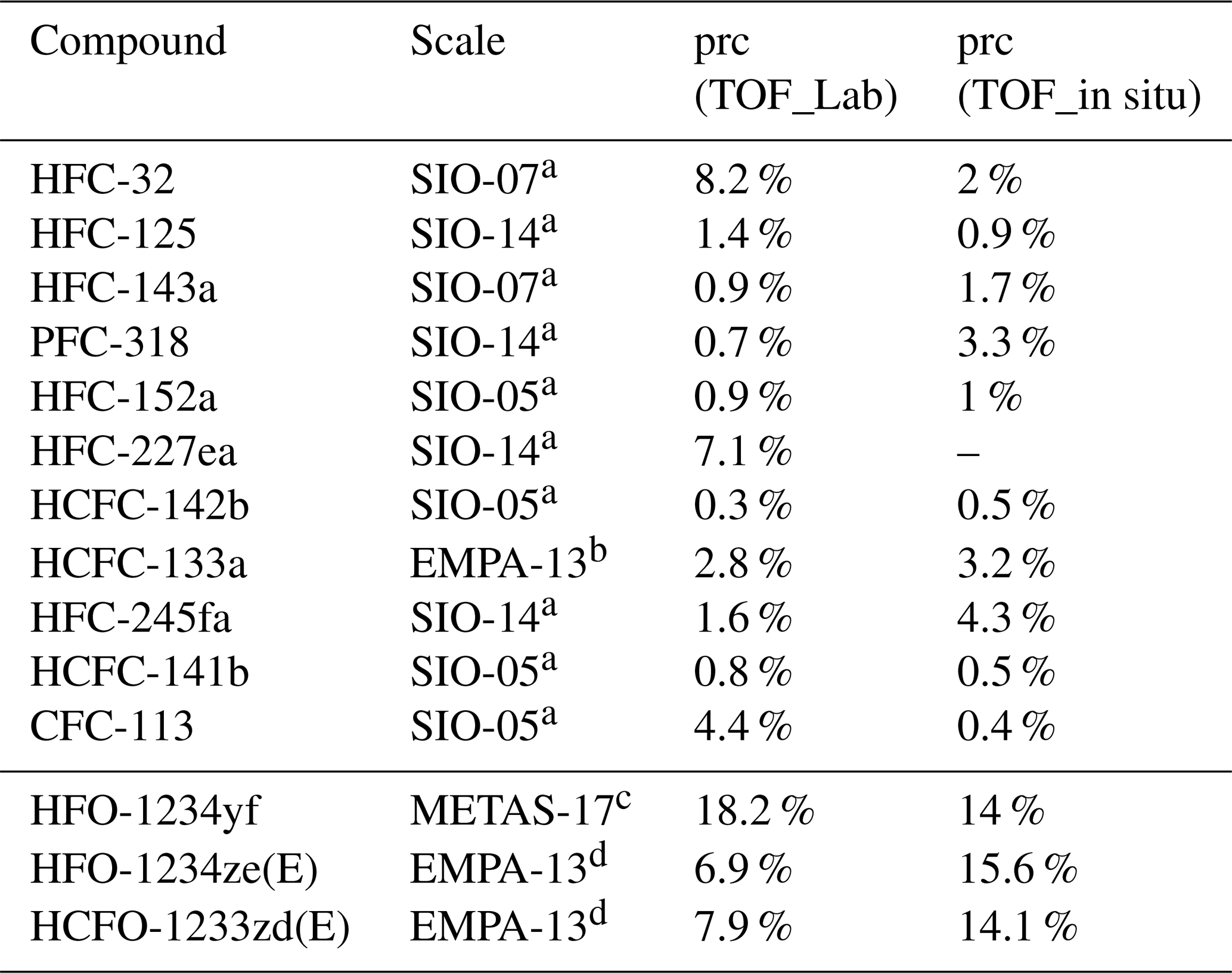
^a Prinn et al. (2000), Prinn et al. (2018). ^b Guillevic et al. (2018). ^c Vollmer et al. (2015b). ^d Vollmer et al. (2015a).

Figure 1 shows a schematic example for the identification of periods of stable rRF, where a random dataset was created. Panel (a) shows the rRF_evalu for two arbitrary substances, a so-called main reference and an evaluation substance, which are both detectable in the used calibration standard. To identify periods of stable rRF_evalu, for each individual measurement the number of measurements with an rRF_evalu that differs by not more than 10 % is counted. Therefore, every single data point was compared to all other data points iteratively. The data point with the highest number of matching data points is used as a reference and all measurements that fall outside the 10 % interval are excluded (shown as grey data points in panel b). If more than one measurement has the same number of matching data points, the case with the lowest standard deviation is selected. In our application, we have arbitrarily chosen a maximum deviation of 10 % as a selection criterion, as it allowed us to retain a sufficient number of measurements while still eliminating data which would have particularly large uncertainty. Depending on the stability of the instrument and the desired results, different criteria could be chosen. Allowing for larger deviations would result in retaining more data with larger uncertainties, while applying a more stringent criterion would result in a dataset with less data yet likely also lower uncertainties. In panels (c) and (d) the evaluation substance is replaced by a third substance, hereafter named test substance, and the rRF_test is plotted. In panel (d) the data point selection determined above is applied to the rRF between test and main substance. For comparison, panel (c) shows the selection that would be obtained if the above procedure was directly applied to the main-test pair of substances. For three outliers with a high peak area ratio and several outliers with low ratios, a mismatch is evident. To choose the best combination of one main reference and one evaluation substance, all possible combinations from the selected substances in Table 1 are investigated and tested for how well they represent known test substances.

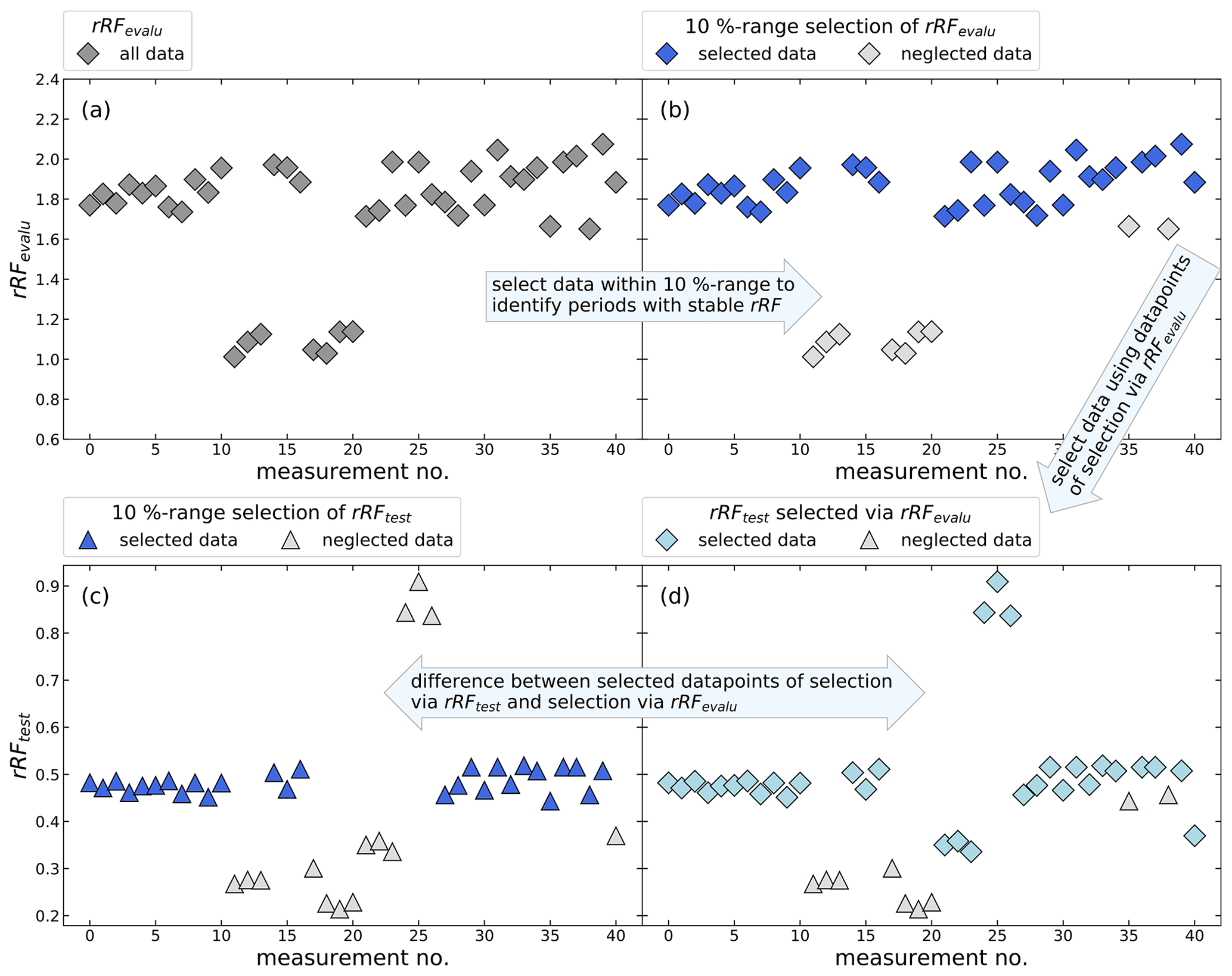
Figure 1 Schematic example using a random dataset of the identification of periods with constant rRF for an undetectable substance in the calibration standard. Panels (a) and (b) show the calculated rRF_evalu of a known main reference and a known evaluation substance. Panel (b) shows which measurements will be selected, excluding measurements where the rRF differs more than 10 %. The resulting selection of measurements should represent the periods of stable rRF_test in panel (c) and (d), where the rRF is determined using the main reference substance and an arbitrary test substance. The aim is to find a main reference and an evaluation substance, which have many measurements with a constant rRF and which will represent the selection of test substances as well as possible.

3.2.2 Evaluation based on weekly sample measurements

To evaluate the stability of the rRF of the laboratory GC–MS setup used to analyse the weekly canister samples, we determined for each pair of substances from the compound selection listed in Table 1 the coefficient of determination (r²) and the mean absolute percentage error (MAPE), defined as

$$\begin{array}{}\text{(6)}& {\displaystyle \frac{\mathrm{1}}{n}}\cdot \sum _{t=\mathrm{1}}^n{\displaystyle \frac{O\left(t\right)-F\left(t\right)}{O\left(t\right)}}\cdot \mathrm{100},\end{array}$$

where n is the number of observations, F(t) is the predicted data as orthogonal distance regression fit forced through the origin and O(t) is the data of the observed peak areas. The r² and the MAPE are both calculated for all calibration gas measurements during the measurement routines of the air samples. Figure 2 shows illustrative correlations of peak areas for HFC-143a (a), HFC-125 (b), and HFC-227ea (c), versus HFC-152a, PFC-318, and HCFC-133a. Except HFC-227ea (column c), the presented substances and their comparisons of peak areas show a good correlation with r²>0.95 % and a MAPE <20 %. Even if the observed substances show a wide range of peak areas, it has to be mentioned that they mostly correlate well, while the observed time period covers nearly 5 years, where system sensitivities have been changed over time. To test which pairs of substances produce the highest correlations, all possible pairs of substances were tested. The obtained values for r² and the MAPE are shown in Fig. 3. Except for HFC-227ea, which shows a mean r² of 0.31 and a mean MAPE of 27 %, the means of r² vary between 0.8 and 0.9 and an average MAPE is below 25 % in all cases.

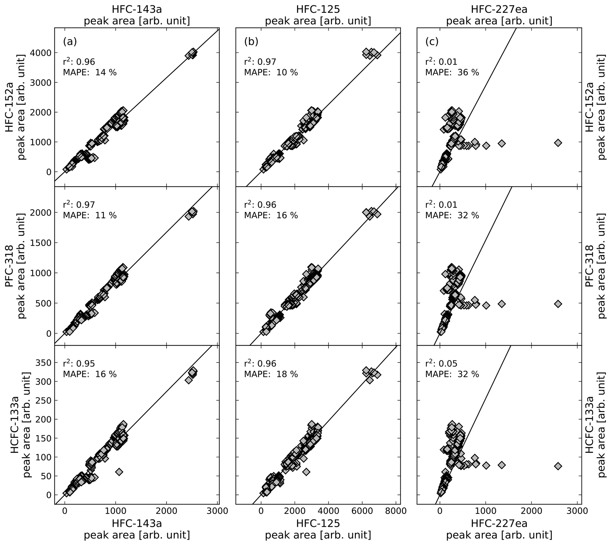
Figure 2 Correlation of peak areas of illustrative substances from calibration gas measurements of phase where calibration cylinder GUF-10 was used, their coefficient of determination (r²) and the mean absolute percentage error (MAPE). Shown are the substances HFC-143a in column (a), HFC-125 in column (b), and HFC-227ea in column (c) and their comparison to HFC-152a (first row), PFC-318 (second row), and HCFC-133a (third row).

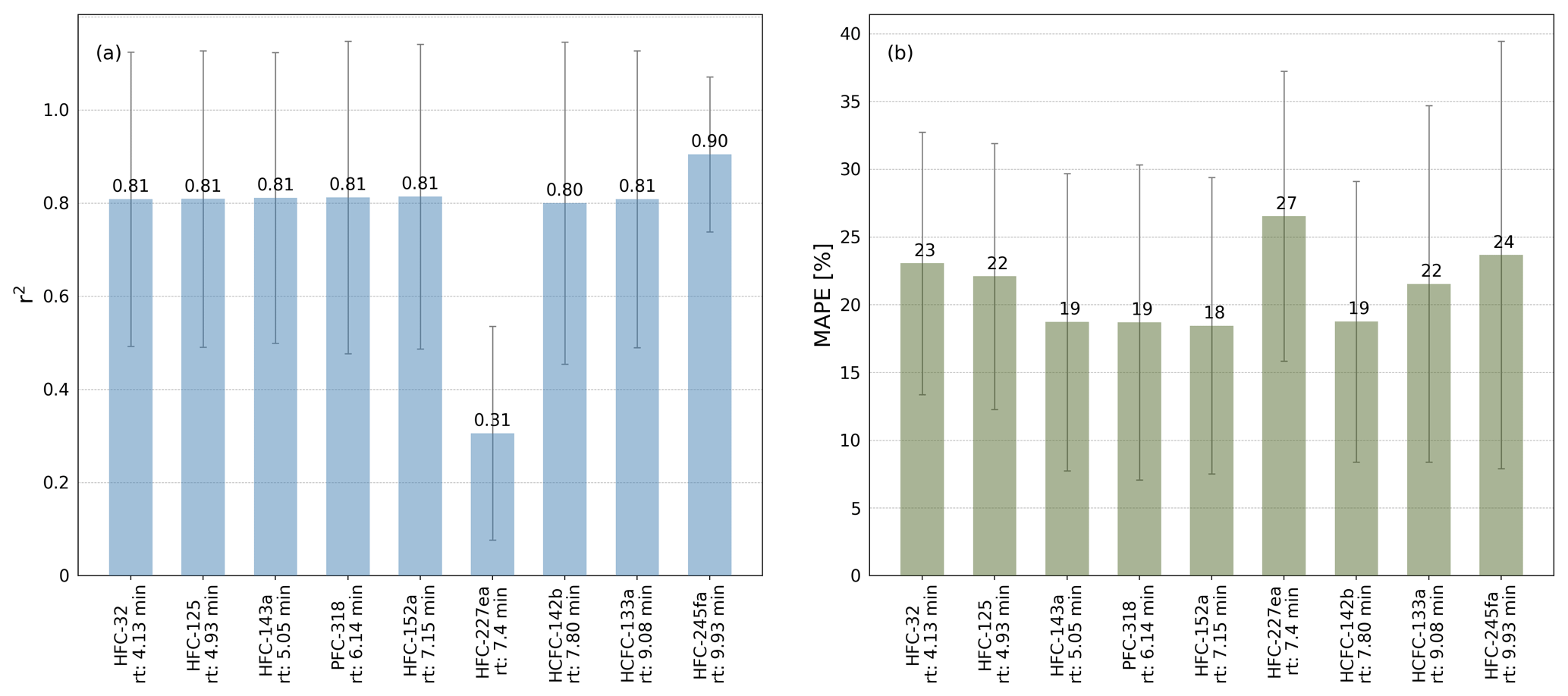
Figure 3 Means of the coefficient of determination (r²) in panel (a) and means of mean absolute percentage error (MAPE) in panel (b) of the comparisons of the peak areas of HFC-32, HFC-125, HFC-143a, PFC-318, HFC-152a, HFC-227ea, HCFC-142b, HCFC-133a, and HFC-245fa to all other substances based on measurements of calibration standards using the laboratory TOF-MS setup in the phase where calibration cylinder GUF-10 was used. Error bars indicate the standard deviations (1σ).

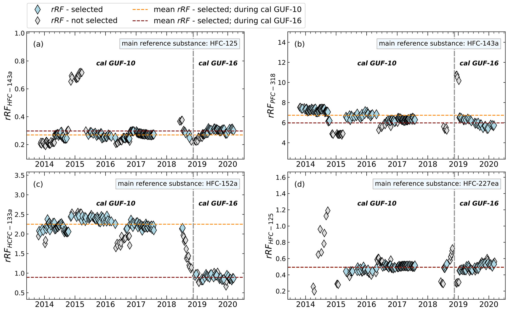
Figure 4 Differences of calculated and filtered rRF of whole-air flask sample measurements during the use of the GUF-10 and GUF-16 calibration standards. As exemplary compounds, different main reference and evaluation substances (rRF_evalu) are shown. The vertical grey dashed line indicates the change of the used calibration gases.

As the rRF is referenced relative to the mole fraction of the measured gas, this value should be independent of the mole fractions and thus should also remain constant after a change of standard, depending on the linearity and any zero off set. Such a change of working standard occurred during the measurement time series discussed here in late 2019. Figure 4 shows this change of standard as a dashed vertical line. While for most combinations the rRF does not show a systematic change, the rRF of HCFC-133a relative to HFC-152a shows a significant shift. However, this shift in rRF started before the change of standard and is thus obviously not related to an inconsistent calibration in the two standard gases used. The reason for this shift is not known, but this is illustrative of the limitations of the indirect calibration method. Under such extreme cases, strong shifts would be observed in the atmospheric measurements and such shifts should thus be treated with care. For other main reference substances, like HFC-125 and HFC-227ea the average relative deviation of rRF is below 8 %, when HFC-152a is excluded as an evaluation substance. It has to be taken into account that in some cases, such outliers may occur applying our rRF filter, which may not be caught by the preprocessed data analysis and its filtering method. Additionally, the number of measurements after selecting the periods of constant rRF should remain as high as possible; for example, using HFC-227ea and HFC-245fa as evaluation substances in combination with HFC-143a as main reference substance or using HFC-245fa as a main reference, more than half of the calibration measurements are excluded, as shown in Fig. 5d and h. As this leads to a significant decrease in the number of air measurements for which an indirect calibration value can be derived, these substances are also less suitable as reference substances.

Figure 5 Illustration of constant rRF data selection, using the standard calibration measurements during the weekly flask sampling measurements, using two different main reference substances (HFC-143a a–d, HFC-245fa e–h) and an evaluation substance (HFC-125). Panels (a) and (e) show results of the application of the 10 % filter. Red data points are excluded as outliers. Panels (b) and (f) illustrate which data of main reference and test substances (here PFC-318) would be chosen applying the resulting selection of panels (a) and (e). Panels (c) and (g) show the result of data selection based on the main reference and the test substance directly. The dashed lines indicate the means of the rRF of the selected data. In panels (d) and (h), vertical bars show percentages of data selected for the respective main reference substance, and coloured symbols show the differences of the relative standard deviations of the rRF of main reference and test substance selected via main reference (HFC-143a in panel d and HFC-245fa in panel h) and all evaluation substances (x axis) between the originally selected rRF via main reference and test substance.

The next step is the identification of periods with a constant rRF. Figure 5 shows the resulting selection of suitable measurement periods for HFC-143a (left column) and HFC-245fa (right column) as main reference substances with HFC-125 as evaluation substance and PFC-318 as test substance. Figure 5a and e show the calculated rRF from October 2013 to October 2018. Figure 5b and f show the resulting data selection for PFC-318 (left, with HFC-143a as main reference, right, with HFC-245fa as main reference). Shown is the rRF of main reference and test substance. Data points which are excluded based on the evaluation substance are represented by red symbols. For comparison, Fig. 5c and g show the selection of data points if the above variability filter would be applied directly to the combination of main reference and test substance. To quantify the precision loss between direct calibration and calibration via an evaluation substance, we compared the relative standard deviations of the resulting dataset as follows: (i) the rRF_test dataset, applying the 10 % filter criterion directly (Fig. 5c and g), and (ii) the rRF_test dataset, using the data points which are selected via the residual rRF_evalu data points applying the 10 % filter criterion (Fig. 5b and f). This is shown for all substance combinations in Fig. 5d and h (coloured points). A small range of standard deviations for a substance indicates more stable data selection and roughly correlates with a high percentage of selected data points as for example for HFC-143a. Figure 5d and h also show the percentage of selected data points for the evaluation substances (blue vertical bars). As pointed out before, HFC-143a showed a high correlation coefficient r² and a low MAPE in comparison to other substances, making it a promising candidate for the main reference substance. Using HFC-143a as main reference substance, on average 49.8 % of data points are used. In the case of HFC-245fa, this decreases to only 34.6 % of data points on average.

In summary, for a good indirect calibration, the main reference and an evaluation substance should show a stable rRF for a large number of measurements and also rRF should be stable with a change of calibration gas. Finally, the rRF of data points selected via main reference and evaluation substance should not vary too much from the rRF of data points selected via main reference and test substance. Based on these criteria, we chose HFC-143a as main reference substance and HFC-125 as evaluation substance. Signal areas of HFC-143a have a high mean r² above 0.8 for all tested substances and one of the smallest mean values of a MAPE with 19 %. After the application of the ± 10 % data selection criterion with HFC-125 as evaluation substance, HFC-143a has more than 50 % of the selected data for six out of the eight tested evaluation substances. Its retention time of 7.15 min is close to that of the three target species HFO-1234yf (6.0 min), HFO-1234ze(E) (6.8 min), and HCFO-1233zd(E) (9.6 min). Using HFC-125 as evaluation substance with HFC-143a, the difference between the standard deviations of the mean rRF selected via the test substances and selected via itself ranges between 1 % and 10 %. HFC-125 also has a large mean r² in comparison to other substances in the calibration gas measurements and the fifth lowest mean MAPE (22 %) (cf. Fig. 3).

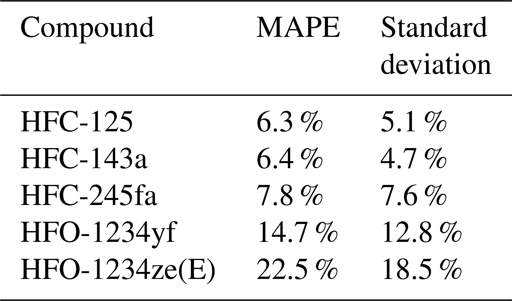
The next step of the method evaluation is the application to several test substances for which results of the indirect calibration can be compared to directly calibrated measurement results. As test cases to apply the indirect calibration method, we chose HFC-32, HFC-227ea, and HFC-245fa. Results are presented in Fig. 6. Shown are time series of directly and indirectly determined mole fractions (left plots) and their correlations (right plots). In this test case, mole fractions of HFC-227ea show the best correlation with r² > 0.9 and a MAPE of 11 % (Fig. 6c and d), whereas for the mole fractions of HFC-32 and HFC-245fa poorer results with r²=0.79 and r²=0.63, respectively, are obtained. The MAPE values, where F(t) is now defined as the indirect calculated mole fractions, and O(t) defined as direct calculated mole fractions (cf. Eq. 6), are given in Table 2. Table 2 shows also the standard deviation of the relative deviations between indirect and calculated mole fractions, to show the spread of the differences between direct and indirect calculated mole fractions. The rRF of HFC-245fa as evaluation substance and HFC-143a as main reference substance has also less than 50 % of selected data within the 10 % filter (cf. Fig. 5), which means that the calculation is applied to a large portion of data for which the criterion of a constant rRF was not met. This underlines how crucial the assumption of constant instrumental sensitivity is for the indirect calibration method.

Table 2 The mean percentage error (MAPE) of directly and indirectly calculated mole fractions and standard deviations of the relative deviations of each data point (direct vs. indirect) for the whole-air flask sample GC–MS measurements for the period from October 2013 to December 2018 (cf. Fig. 6). As main reference, HFC-143a is used; as evaluation reference, HFC-125 is used.

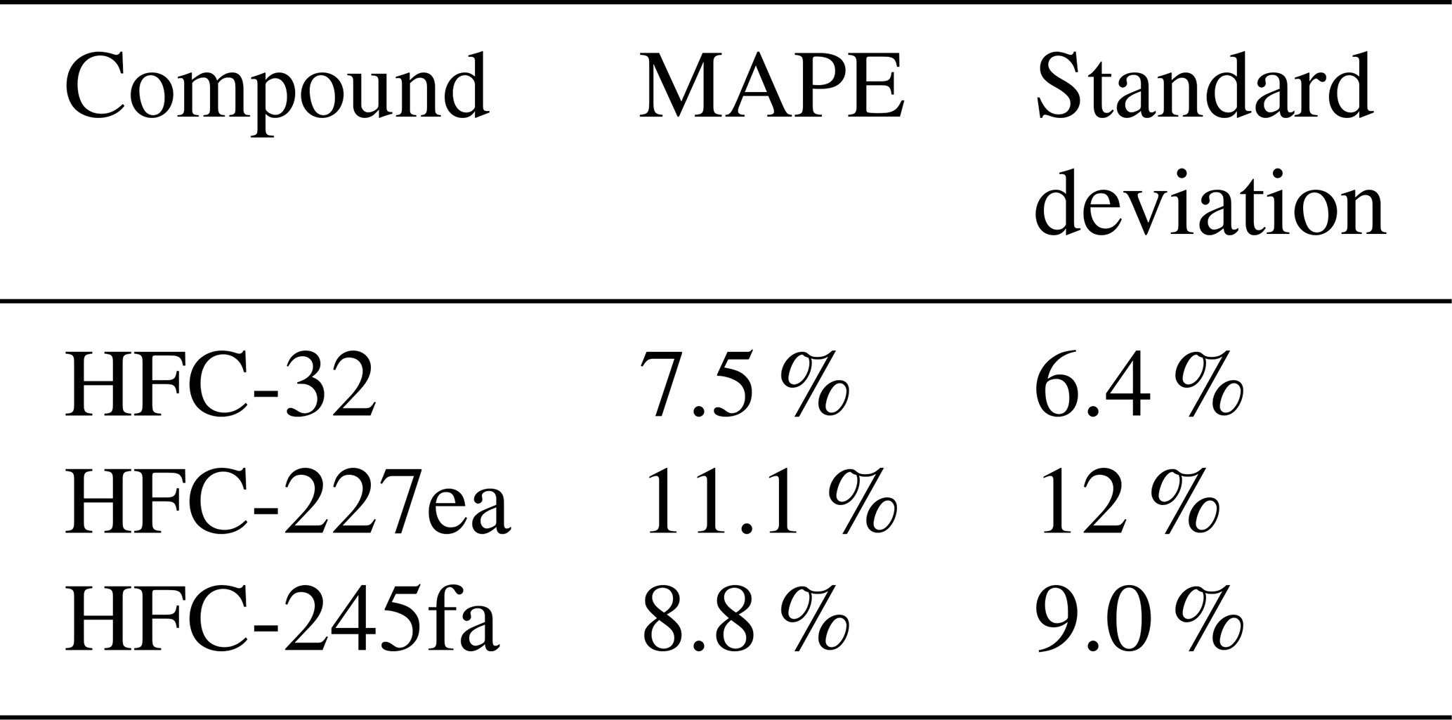
Figure 6 Time series (a, c, e) and correlations (b, d, f) of the mole fractions of HFC-32, HCFC-227ea, and HFC-245fa calculated directly (yellow symbols) and indirectly (blue symbols) for the weekly flask sample measurements. HFC-143a was used as main reference substance and HFC-125 as evaluation substance to select data with constant rRF. Error bars, which indicate the measurement precisions, are included but are often smaller than symbol size.

3.2.3 Evaluation based on in situ measurements

For the application on the continuous in situ measurements, the preselection of main reference and evaluation substances yields different results. This implies a strong system dependency of the method and a need to evaluate appropriate substances for indirect calibration per system. In our case we can observe such a different behaviour in substance selection for HFC-152a. While it is not applicable for the indirect calibration method (cf. Fig. 4), using the in situ measurement setup it is our best selection within the training dataset. Figure 7 shows the results of the data selection procedure for the in situ GC–MS at Taunus Observatory, using HFC-152a (left) and HFC-245fa (right) as main reference substances for the period May 2018 through March 2019. Shown are daily mean values for simplicity, but 2-hourly data were used for all calculations. Histograms in Fig. 7d and h show that a large percentage of data meet the filter criterion and a larger fraction of data is selected from the in situ measurements than from during the weekly flask sample measurements. This could be due to the shorter time period covered by the in situ data and also due to the continuous measurements in contrast to flask measurements in the laboratory, where the instrument is in standby for longer time periods. HFC-152a as main reference has a high overlap within the 10 % range with the other substances, with a mean of 78.9 % data selected. For HFC-245fa, this is only 70.1 %.

Figure 7 Same as Fig. 5 but for the continuous in situ measurements at Taunus Observatory using main reference substances HFC-152a (a–d) and HFC-245fa (e–h) and PFC-318 as evaluation substance.

Figure 8 shows the comparison of directly and indirectly calculated relative responses and mole fractions for HFC-125, HFC-143a, and HFC-245fa. Again, daily mean values are shown for simplicity, while all calculations were performed for the air measurements every second hour. For the continuous measurements, HFC-152a is used as a main reference and PFC-318 as a evaluation substance. As was the case for the flask sample measurements, some features of the time series are caught well. Especially shorter-term variations are well captured, while long-term trends between the directly and indirectly calculated mole fractions sometimes show systematic differences between the directly and indirectly determined methods. This is caused by long-term drifts in the rRF and shows clearly that the indirect calibration measurement should only be applied when investigating very large long-term trends when no directly calibrated measurements are available. The average relative differences are given in Table 3.

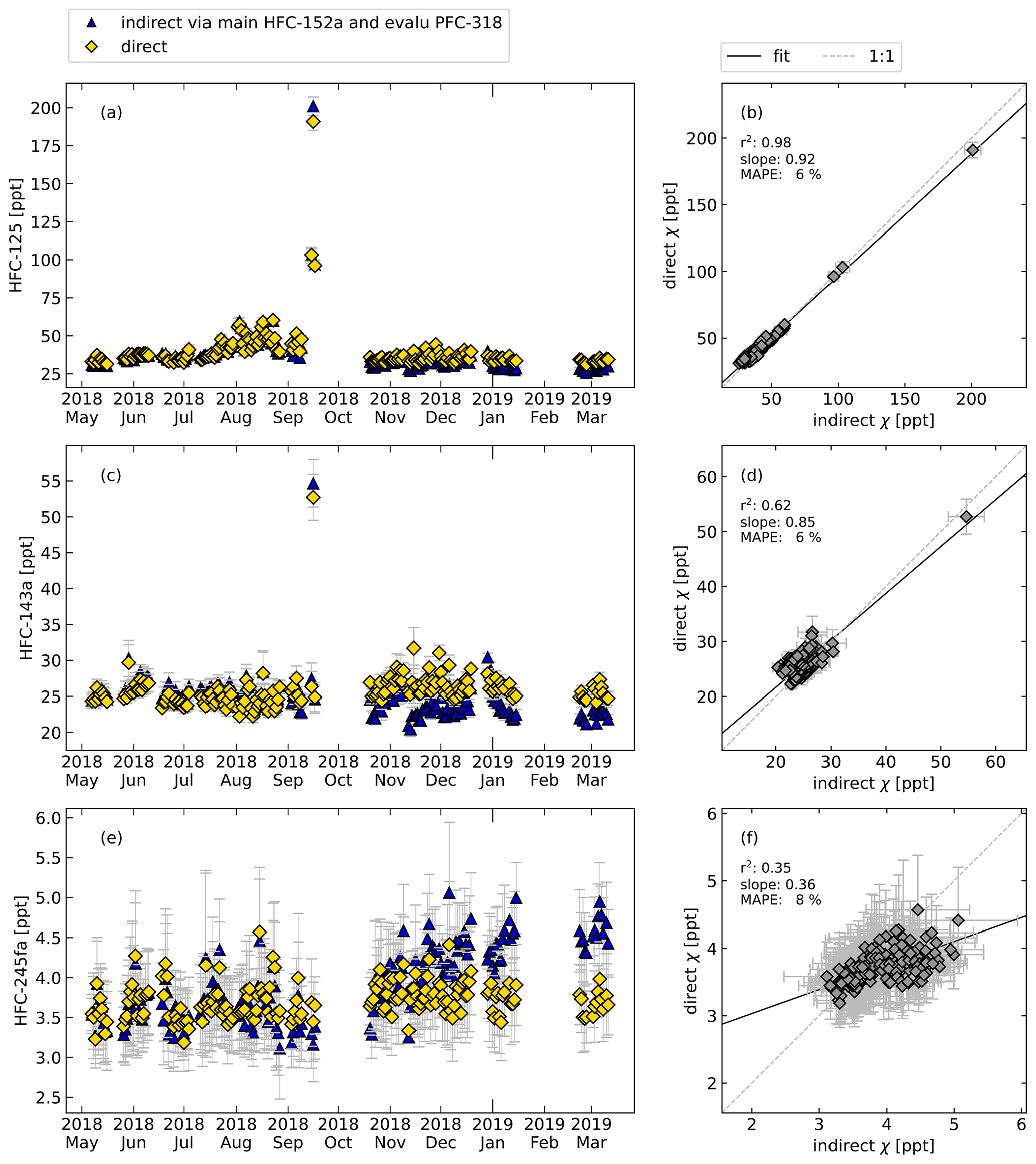
Figure 8 Same as Fig. 6 but for the continuous in situ measurements at Taunus Observatory using GC–MS and for the following compounds: HFC-125, HFC-143a, and HFC-245fa, calculated directly (yellow symbols) and indirectly (blue symbols). Here, HFC-152a was used as main reference substance and PFC-318 as evaluation substance to select data with constant rRF. For reasons of simplified illustration, daily means are shown. The error bars indicate the standard deviations of the measurements of 1 d and thus reflect the daily atmospheric variability and do not include systematic errors due to the indirect calibration method.

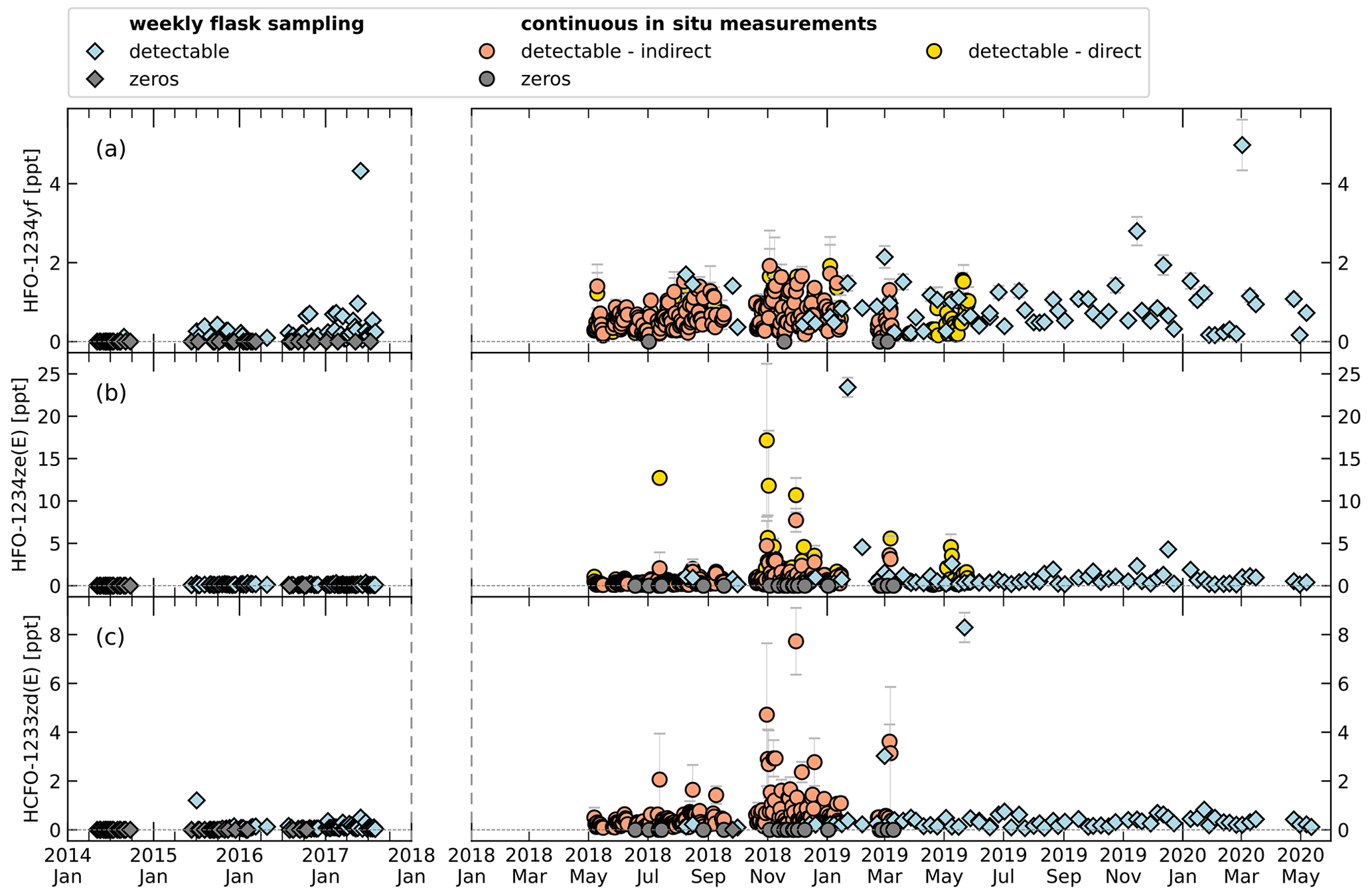
Figure 9 Time series of mole fractions of HFO-1234yf (a), HFO-1234ze(E) (b), and HCFO-1233zd(E) (c) at TOB. Symbol shape indicates flask sampling (diamonds) and in situ measurement (circles). Grey symbols represent mole fractions below detection limit (cf. Tables 2 and 3). Data of weekly flask sampling are indirectly calibrated mole fractions before January 2018 and directly calibrated values after. For the in situ measurements, indirectly and directly calibrated mole fractions are indicated by colour (orange and yellow). Note the change in x-axis scaling after January 2018 because of increased data frequency. Data of in situ measurements show daily means. Error bars for weekly flask sampling show the 1σ standard deviation of the measurements for one sampling. Error bars for the in situ measurements show the standard deviation of the average of measurements over 1 d.

Figure 10 Same as Fig. 9 but zoomed in to visualise small mole fractions better.

4 Application of indirect calibration method to short-lived synthetic halocarbons

As the indirect calibration method has shown satisfactory results for the test substances, we apply it to the short-lived compounds HFO-1234yf, HFO-1234ze(E), and HCFO-1233ze(E). For these compounds, the direct calibration is limited to parts of the time series which were calibrated with gases containing these substances at sufficiently high mole fractions.

Figure 9 shows a time series of measurements with the two GC-TOF-MS systems from January 2014 to May 2020 for the weekly whole-air sampling measurements and from May 2018 to May 2019 for the continuous in situ measurements. To visualize small mole fractions, Fig. 10 shows the same data zoomed in. A comparison of direct and indirect calibrated data can only be performed for the continuous in situ measurements, where the calibration gas used until March 2019 contained detectable amounts of HFO-1234yf (0.149 ppt) and HFO-1234ze(E) (0.199 ppt). The average relative differences of that comparison are given in Table 3. For HFO-1234yf, the mole fractions differ by around 24.3 %; for HFO-1234ze(E), the relative average difference is 19.5 %.

Table 3 The mean percentage error (MAPE) of directly and indirectly calculated mole fractions and the standard deviations of the relative deviations of each data point (direct vs. indirect) for the in situ GC–MS measurements for the period from May 2018 to March 2019 (cf. Fig. 8). As main reference, HFC-152a is used; as evaluation reference, PFC-318 is used.

Data from the weekly flask sampling (cf. Table 4) show increasing detection frequency for the investigated H(C)FOs since 2014, as seen in Vollmer et al. (2015a). In 2014 only HFO-1234yf was detected. Until 2018 the detection frequency of HFO-1234yf and HCFO-1233zd(E) increased continuously up to 100 %, whereas in 2019 they were detected in 96 % and 98 % of measurements. From 2015 to 2019, HFO-1234ze(E) mostly shows a detectability of 100 %, except for 2016 (92 %) and 2019 (98 %). From 2014 to 2019, weekly mole fractions range between 0–5 ppt (0–2 ppt calculated indirectly) for HFO-1234yf. Its annual mean mole fractions increased from 0.03 ppt in 2014 (calculated indirectly) to 0.81 ppt in 2019 (calculated directly). The high mean mole fraction for the indirectly calculated data of HFO-1234yf in 2018 (1.23 ppt) could be due to only four samples being available between August and October, where weekly mole fractions seem to be higher due to an annual cycle. For HFO-1234yf(E) weekly mole fractions from 2015 to 2019 mostly range between 0–2 ppt, except for a few outliers. Annual mean mole fractions of HFO-1234ze(E) increased from 0.12 ppt in 2015, calculated indirectly, to 1.27 ppt in 2019, calculated directly. Also, HCFO-1233zd(E) shows increasing annual mean mole fractions, from 0.1 ppt in 2015, calculated indirectly, to 0.51 ppt in 2019, calculated directly. The annual mean mole fractions of all three H(C)FOs at TOB are in between typical mole fractions observed at the urban Dübendorf site and the clean air site at Jungfraujoch in Switzerland (Vollmer et al., 2015a, and update by Vollmer et al., 2015a, unpublished, Martin Vollmer, private communication, 2019).

Data from the in situ measurements (cf. Table 5) show a variation of detectable amounts between 96 % and 98 % for HFO-1234yf and between 91 % and 93 % for HFO-1234ze(E). The means of HFO-1234yf data calculated indirectly do not differ more than 15 % from the direct calculated data (for 2019 direct and indirect). Whereas HFO-1234ze(E) shows a large deviation with maximal 44 % for the data in 2018. These larger deviations could be caused by the small peak of HFO-1234ze(E) in the calibration gas used from May 2018 to March 2019. The mean values of both substances, independently if calculated directly or indirectly, do not show an increase or decrease over the short time period of less than 1 year which is covered by the in situ data. The indirect mean values in 2018 for both substances compared to the indirect calculated substances using the whole-air flask sampling data are lower (mean HFO-1234yf mole fraction is 0.57 ppt lower, HFO-1234ze(E) shows a 0.11 ppt lower mean mole fraction). But as mentioned previously, this could be caused by an unequal time distribution of the data. Also, this could cause the other deviations between the in situ and whole-air flask measurements. Such deviations are to be expected due to possible long-term drifts in rRF, again emphasising the point that the indirect calibration method is better suited to investigate short-term variability in ambient air measurements than for the detection of long-term trends. However, typical mole fractions are also in between typical mole fractions observed at the urban Dübendorf site and the clean air site at Jungfraujoch, both in Switzerland (Vollmer et al., 2015a, and update by Vollmer et al., 2015a, unpublished, Martin Vollmer, private communication, 2019).

Table 4 Mean and median observed mole fractions (in ppt), number of observations, and the percentage of detectable peaks per year of HFO-1234yf, HFO-1234ze(E), and HCFO-1233ze(E) in the whole-air flask samples. Data between 2014 and 2018 are calculated indirectly and are in italic, whereas data from October 2018 onwards are calculated directly. The indirectly estimated mole fractions are calculated using the indirect calibration approach, with HFC-143a as main reference substance and HFC-125 as evaluation substance. Mean and median values include measurements with undetectable mole fractions, as is performed in Vollmer et al. (2015a). Instead of assigning those a value of zero, values equal to half of the detection limits were assigned to them. The limits of detection (LODs), which are calculated as the 1.5-fold noise of each chromatogram, are 0.04 ppt (HFO-1234yf), 0.06 ppt (HFO-1234ze(E)), and 0.05 ppt (HCFO-1233zd(E)).

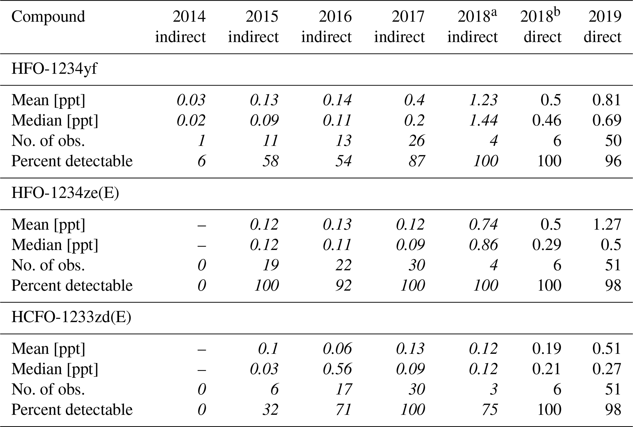
^a Data of 2018 are calculated indirectly until 23 October. ^b Data of 2018 are calculated directly since 24 October, using the calibration standard GUF-16.

Table 5 Same as Table 4 but for the continuous in situ measurements at TOB from May 2018 to May 2019 for HFO-1234yf and HFO-1234ze(E). The indirect mole fraction estimations from May 2018 to March 2019 are based on HFC-152a as main reference substance and PFC-318 as evaluation substance. The limits of detection (LODs), which are calculated as the 1.5-fold noise of each chromatogram, are 0.02 ppt for HFO-1234yf and 0.01 ppt for HFO-1234ze(E) for the in situ measurements.

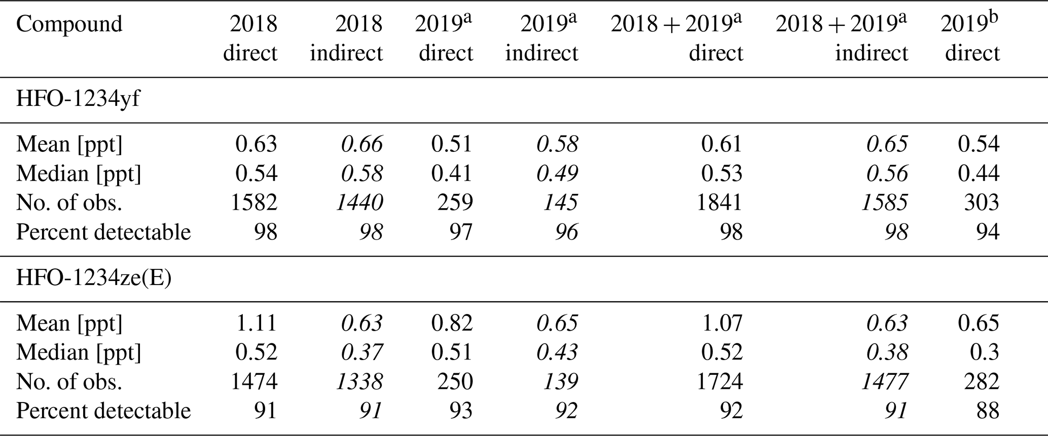
^a Data of 2019 are calculated directly and indirectly until March 2019. ^b Data of 2019 are calculated directly only since March 2019, using the calibration standard GUF-17.

5 Summary and conclusions

Non-target analysis using full-scanning MS offers the opportunity to detect and quantify species in the atmosphere retrospectively. However, as GC is a relative measurement technique, knowledge of the mole fraction of the retrospectively analysed species in the calibration gas is required. Often the species of interest is either not detectable in the calibration gas or the mole fraction in the calibration gas is not known. For such cases, we have developed an indirect calibration approach which relies on the assumption that the relative sensitivity of the analytical system to two species changes in a similar way so that their ratio would be constant in time, even if the absolute sensitivity of the system changes. In this case, quantification may be performed using the measurement of a reference species and the ratio of the relative sensitivities of target and reference compound, provided that the absolute value of the relative response of the species is derived retrospectively. In order to evaluate the stability of the relative responses of two such species, we tested the approach using species with concentrations that are known in the calibration gas. We suggest that it is useful to use an evaluation substance to select periods when relative responses of the measurement system are rather stable. Further, it is likely that using reference species with similar retention times as the target species provides more stable results, which should be investigated with a larger number of training substances. The training dataset used in this work could not confirm that. By analysing correlations and variabilities of the relative responses, we identify the combination of a main reference and an evaluation substance which yield the minimum number of rejected data points of different target gases. Furthermore, we have chosen to include only time periods where the relative response of the reference substance and the evaluation substance are stable within 10 % in the analysis. A good combination of reference and evaluation substance should thus yield small deviations between direct and indirect calibration for a wide range of compounds while also retaining a maximal fraction of measurements based on the filter criterion of maximum deviation in relative response factor, if possible.

This procedure with the 10 % criterion is applied to two different datasets for testing. The first dataset is a measurement time series of flask samples collected at the Taunus Observatory on the Kleiner Feldberg near Frankfurt in Germany. This dataset has been evaluated for the time period from October 2013 to December 2018. The second dataset is from in situ measurements at the Taunus Observatory using an automated GC system with TOF-MS detection. This dataset has been evaluated for the time period from May 2018 to March 2019. Comparing the data points of each measurement, calculated directly and indirectly, we found the following averaged relative differences of mole fractions for the investigated substances: for the long-term flask data, we find relative differences between directly and indirectly calibrated mole fractions of different gases ranging between 8 % and 11 %. For the in situ data, differences between directly calibrated and indirectly calibrated mole fractions ranged between about 6 % and 23 %.

Based on these differences between directly calibrated and indirectly calibrated values of up to 23 %, we conclude that the indirect calibration method is not suited for detection of small trends of long-lived gases in the atmosphere, which are often of the order of less than 1 % yr⁻¹. However, for species with large trends where no direct measurements are available, this method can provide the correct order of magnitude of atmospheric mole fractions in the past. A further interesting application is the measurement of short-lived gases, which are expected to show high variability in the atmosphere. For such gases, both correct orders of magnitude and also the frequency at which they are observable can be derived. In order to confirm the validity of the indirect calibration approach, it will be useful to maintain aliquots of calibration gases so that these can be calibrated retrospectively, allowing us to confirm the stability of relative response factors for species which are detectable and stable in the calibration gas over a longer time period.

Examples for species where the indirect calibration is useful are the unsaturated HFOs and HCFOs, which have recently been introduced as replacement compounds for long-lived hydrofluorocarbons. These gases are short lived with local lifetimes of less than a month and are increasingly used in, for example, mobile air conditioning. The three H(C)FOs, HFO-1234yf, HFO-1234ze(E), and HCFO-1233zd(E), have been detectable at an increasing frequency in our ambient air chromatograms. We have thus applied the indirect calibration method to both the flask measurements and the in situ measurements of H(C)FOs. For the flask measurements, we show that the frequency at which measurable peaks are observed at Taunus Observatory increases with time. All H(C)FOs are present in nearly all flask samples collected at the Taunus Observatory since early 2018, while samples from the year 2014 only showed very occasional measurable concentrations of HFO-1234yf. Consequently, typical mole fractions increased from below 0.1 ppt in 2014 (indirectly calibrated) to median values between 0.25 ppt for HCFO-1233zd(E) and 0.7 ppt for HFO-1234yf in 2019, based on a direct calibration. While the direct calibration is also preferable, the indirect calibration offers additional useful information in this case. This observed increase in the mole fractions and the frequency of observations is in line with the observations by Vollmer et al. (2015a) and an update by Vollmer et al. (2015a) (unpublished, Martin Vollmer, private communication, 2019) at the remote station of Jungfraujoch. As expected, the mole fractions observed at Taunus Observatory are in between those reported for the remote station of Jungfraujoch and the urban station of Dübendorf in Switzerland (Vollmer et al., 2015a, and update by Vollmer et al., 2015a, unpublished, Martin Vollmer, private communication, 2019).