A systematic assessment of water vapor products in the Arctic: from instantaneous measurements to monthly means

Water vapor is an important component in the water and energy cycle of the Arctic. Especially in light of Arctic amplification, changes in water vapor are of high interest but are difficult to observe due to the data sparsity of the region. The ACLOUD/PASCAL campaigns performed in May/June 2017 in the Arctic North Atlantic sector offers the opportunity to investigate the quality of various satellite and reanalysis products. Compared to reference measurements at R/V Polarstern frozen into the ice (around 82^∘ N, 10^∘ E) and at Ny-Ålesund, the integrated water vapor (IWV) from Infrared Atmospheric Sounding Interferometer (IASI) L2PPFv6 shows the best performance among all satellite products. Using all radiosonde stations within the region indicates some differences that might relate to different radiosonde types used. Atmospheric river events can cause rapid IWV changes by more than a factor of 2 in the Arctic. Despite the relatively dense sampling by polar-orbiting satellites, daily means can deviate by up to 50 % due to strong spatio-temporal IWV variability. For monthly mean values, this weather-induced variability cancels out, but systematic differences dominate, which particularly appear over different surface types, e.g., ocean and sea ice. In the data-sparse central Arctic north of 84^∘ N, strong differences of 30 % in IWV monthly means between satellite products occur in the month of June, which likely result from the difficulties in considering the complex and changing surface characteristics of the melting ice within the retrieval algorithms. There is hope that the detailed surface characterization performed as part of the recently finished Multidisciplinary drifting Observatory for the Study of Arctic Climate (MOSAiC) will foster the improvement of future retrieval algorithms.

1 Introduction

Water vapor plays an important role in the hydrological cycle of the Arctic as a source for cloud and fog formation and by its effects on the energy budget via condensation–evaporation and radiative transfer (Vihma et al., 2016). For the Arctic climate, water vapor is of particular interest as it could contribute to Arctic amplification by enhancing downwelling longwave radiation (Ghatak and Miller, 2013) and providing the moisture source for precipitation. Investigating relative contributions of the different feedback processes is still under debate and the focus of current research (e.g., Wendisch et al., 2017; Serreze and Barry, 2011).

Despite its importance, the Arctic suffers from a lack of reliable water vapor measurements due to the limited number of surface stations. Thus, studies aiming at the detection of changes in the water vapor distribution mainly make use of reanalyses and radiosondes (e.g., Serreze et al., 2012; Dufour et al., 2016; Rinke et al., 2019). The latter are limited to land areas and concentrated in North America and Europe. Furthermore, measurements at low temperature are especially challenging, and the corrections of sensor time lag and radiation dry bias are best addressed by using Global Climate Observing System (GCOS) Reference Upper-Air Network (GRUAN) processing (Dirksen et al., 2014). While polar-orbiting satellite observations have – by definition – good spatio-temporal coverage in the Arctic, different factors make measurements of water vapor rather challenging there. Techniques relying on solar radiation, e.g., the near-infrared product of the Moderate Resolution Imaging Spectroradiometer (MODIS), are not available during polar night and need reflective surfaces such as sun glint over oceans. The occurrence of clouds hinders water vapor measurements both for solar and thermal infrared (IR) techniques. However, even under clear sky conditions the retrieval is difficult due to the low water vapor amounts and complex, mixed ice, snow and water surface conditions, especially in the marginal sea ice zone which is also affecting passive microwave (MW) measurements.

With their capability to gain information on water vapor under cloudy conditions, low-frequency microwave imager measurements now available for more than 40 years have been fundamental to establishing long-term climatologies of the vertically integrated water vapor (IWV) over the ice-free oceans (Mears et al., 2018; Schröder et al., 2016). To overcome the issue of the highly variable surface emissivity in the polar regions, IWV retrieval from higher microwave frequencies, e.g the Microwave Humidity Sounder (MHS) at millimeter wavelengths, routinely measured by microwave sounders has been proposed (Perro et al., 2016; Scarlat et al., 2018; Triana-Gómez et al., 2020). With the launch of infrared spectrometers including several thousands of channels, i.e., the Atmospheric Infrared Sounder (AIRS) and the Infrared Atmospheric Sounding Interferometer (IASI), enhanced profiling capabilities for water vapor have been added, and approaches for the combination with microwave measurements are used to mitigate cloud effects. Especially AIRS has been used to study Arctic water vapor, including humidity inversions (Devasthale et al., 2016).

In order to quantify the state of the art in water vapor products being constructed for climate applications, the Global Energy and Water Exchanges (GEWEX) Water Vapor Assessment (G-VAP) was initiated in 2011. In the framework of G-VAP, an archive of long-term data records of water-vapor-related essential climate variables (including IWV) was compiled from satellites and reanalyses (Schröder et al., 2018). When looking at IWV variability around the globe, Schröder et al. (2016) found the highest relative standard deviation (SD) between long-term data sets in the polar regions. Thus, it is no surprise that strong discrepancies in the pattern and magnitude of water vapor trends in the Arctic still exist (Rinke et al., 2019).

This study contributes to the second phase of G-VAP by thoroughly investigating the quality of satellite and reanalysis IWV products in the Arctic by making use of the ACLOUD/PASCAL campaigns (Wendisch et al., 2019) performed in the surroundings of Svalbard, including over sea ice in May/June 2017. This period is well suited as it marks the transition period between cold air masses with low IWV to the summer state by warm and moist intrusions from mid-latitudes. The occurrence of three atmospheric rivers (ARs) during ACLOUD/PASCAL affecting Svalbard provides an interesting opportunity to investigate the impacts of high spatio-temporal water vapor variability. ACLOUD/PASCAL also provided enhanced radiosonde measurements from Ny-Ålesund, Svalbard and a connection to a sea ice camp at the research icebreaker Polarstern at about 82^∘ N for evaluation of satellite and reanalysis products.

In the past, few water vapor intercomparison studies have been performed and mainly addressed a limited set of sites and products (Alraddawi et al., 2018; Pałm et al., 2010; Perro et al., 2016; Weaver et al., 2017). Here we aim to address IWV performance for five frequently used global reanalyses including ERA5, the latest climate reanalysis produced by the European Centre for Medium-Range Weather Forecasts (ECMWF), and five satellite products (Sect. 2). In this exercise, we assess water vapor uncertainty from instantaneous (Level 2) to monthly (Level 3) products for the Arctic North Atlantic sector which have different spatio-temporal characteristics (Sect. 3). First, we use reference IWV data from radio soundings and continuous ground-based measurements by the global navigation satellite system (GNSS) and microwave radiometers (MWR) to evaluate the quality of water vapor products on an instantaneous and local scale (Sect. 4.1). Secondly, we move to the spatial distribution and analyze how realistic the spatio-temporal distribution is described by the different data sets on a daily basis (Sect. 4.2). Finally, we aim to connect to climate applications by investigating how uncertainties stemming from the individual measurements, instrument limitations and sampling patterns transfer to the monthly scale (Sect. 4.3). The assessment is concluded with a discussion and outlook of future work (Sect. 5).

2 Data

The ACLOUD and PASCAL campaigns (Wendisch et al., 2019) concentrated their observational efforts on Svalbard and the Fram Strait in May and June 2017. Most important for our study are the measurements on board the R/V Polarstern frozen into the ice (around 82^∘ N, 10^∘ E) and the Alfred Wegener Institute for Polar and Marine Research and the French Polar Institute Paul Emile Victor (AWIPEV) research station at Ny-Ålesund (78.92^∘ N, 11.92^∘ E; 2 $\mathrm{m}\mathrm{a}.\mathrm{s}.\mathrm{l}.$). At both locations, frequent radiosondes were launched, and continuous IWV observations by MWR were performed. In addition, sensor synergy provides detailed cloud characteristics (Nomokonova et al., 2019a) showing 75 % (83 %) monthly mean cloud fraction in May (June) for Ny-Ålesund and 88 % during the ice camp. Low-level clouds were the dominant cloud type.

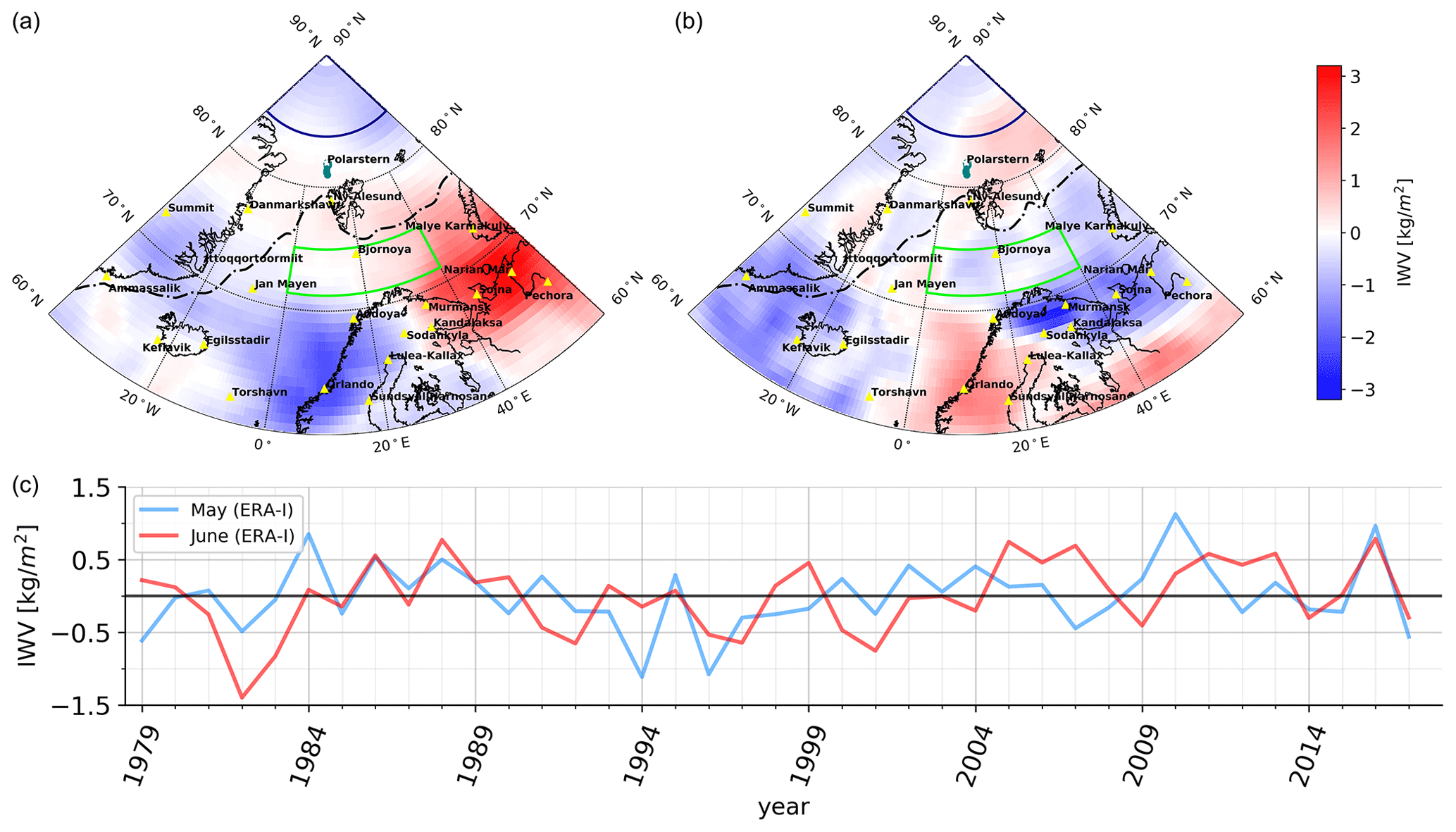
Figure 1 Study area and location of reference stations together with map of IWV anomaly with respect to ERA-Interim long-term climatology (1979–2016) for May (a) and June (b) 2017. Yellow triangles show radiosonde stations. Average sea ice margin is given as dashed black line. Two areas studied in detail are indicated in dark blue (central Arctic) and dark green (open ocean); (c) time series of IWV anomaly averaged over study area (60–90^∘ N, 40^∘ W–60^∘ E) for May and June from 1979 to 2017.

Aumann et al. (2003)Scarlat et al. (2017)Noël et al. (2008)August et al. (2012)Boukabara et al. (2011)Gao and Kaufman (2003)Saha et al. (2014)Hersbach et al. (2020)Dee et al. (2011)Kobayashi et al. (2015)Gelaro et al. (2017)

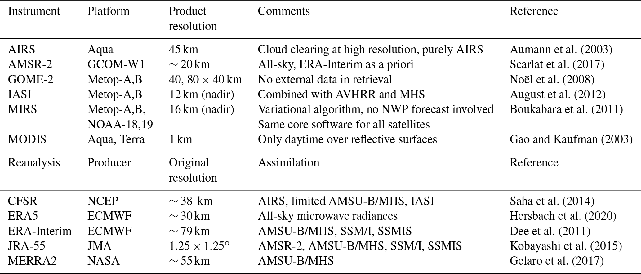
Table 1 Overview of water vapor products used in this study and their nominal resolution. Note that for cross-track imagers (e.g., IASI, MHS) the spatial resolution is highest for nadir and decreases with scan angle.

To broaden the scope of our study, we enlarge our study area to the North Atlantic sector (40^∘ W to 60^∘ E) of the Arctic, defined as north of 60^∘ N (Fig. 1). This area is particularly challenging for satellite retrievals as it includes land, ocean and sea ice surfaces. Therefore, also assimilation of satellite radiances is limited, and as few stations launch radiosondes on a regular basis (Fig. 1), reanalyses are strongly dependent on the underlying model (Lindsay et al., 2014). Compared to the long-term climatology from ERA-Interim (Dee et al., 2011), both May and June 2017 were slightly drier when averaging over the full region, though some areas with moister conditions are evident, e.g., northern Russia in May. For the reference sites at R/V Polarstern and Ny-Ålesund, conditions were close to the long-term mean. The 17 radiosonde stations available in the area include both below- and above-normal conditions. The long-term record (Fig. 1) also indicates the strong inter-annual IWV variability even when averaged over such a large area, making the detection of trends challenging. While in the last 4 years anomalies for May and June were in phase, this has not always been the case in the past. For the spatial comparison of the different satellite and reanalysis products (Table 1), we only show the results for June 2017, while the ones for May 2017 are provided in the Appendix​​​​​​​.

For most of the products IWV is not a directly measured quantity but derived by integrating the vertical humidity profile. In this exercise differences between products can occur due to differences in the vertical sampling and the definition of the lower–upper boundary. The first point is of special relevance for radiosonde measurements and model profiles when strong vertical moisture gradients occur, e.g., during moisture inversions, which are frequent in the Arctic (Naakka et al., 2018). This effect can lead to differences between high-resolution radio soundings and those only using main pressure levels of several kilograms per square meter for individual profiles. The second effect mainly concerns the lower boundary as a height difference between two products can cause systematic biases and is most important in orographically structured terrain where the effective footprint of models and satellite products causes different average elevations. As a rule of thumb a height difference of 100 m in the presence of 5 g m⁻³ absolute humidity (typical maximum for the Arctic) causes an IWV difference of 0.5 kg m⁻². Similarly, synoptic pressure deviations can be problematic (Divakarla et al., 2006) when vertical profiles are provided on fixed pressure grids.

2.1 Satellite products

In total, six satellite products available from polar-orbiting satellites operating in different parts of the electromagnetic spectrum are evaluated. Purely microwave information is used by the Advanced Microwave Scanning Radiometer 2 (AMSR2) and the Microwave Integrated Retrieval System (MIRS). The infrared spectrometer IASI L2 PPFv6 product also incorporates information by microwave sounders. For AIRS, a combined MW–IR product is also available. However, here we use the AIRS-only product (AIRS L2 v6 IR-Only) as this can illustrate the effect of degraded or missing collocated microwave measurements. The Global Ozone Monitoring Experiment 2 (GOME-2) makes use of spectral solar reflectance measurements. For these five satellite products orbital data are aggregated to daily and monthly means. MODIS, which uses near-infrared reflectances, provides valid retrievals with much lower sampling than the others, and therefore only its monthly mean IWV product is shown for completeness. An overview of the products is given in Table 1.

2.1.1 AIRS

Launched in May 2002 on board the Aqua satellite, AIRS (Aumann et al., 2003) measures radiation emitted from the atmosphere and Earth's surface in 2378 wavelength channels between 3.74 and 15.4 µm. The cross-track scanning instrument has a spatial resolution of 13.5 km in nadir, decreasing to 31.5 km on the edges of the 1650 km broad swath. In this paper, the AIRS Version 6 Level 2 standard product (AIRS L2 v6 IR-Only) for orbital data with a 45 × 45 km horizontal resolution is used.

The AIRS water vapor profile product is based on a physical retrieval algorithm using AIRS IR radiances only and no MW information. One of the first steps is to apply a cloud clearing to the measured AIRS radiances. The retrievals of geophysical parameters are performed sequentially using the clear column radiances and an initial state being derived from a neural network approach (Susskind et al., 2014). Each geophysical parameter retrieval uses its own set of AIRS channels: for the water vapor profile retrieval, 41 channels in the spectral ranges from 1310 to 1605 and 2608 to 2656 cm⁻¹ are taken into account. IWV is directly provided in the operational product (totH2OStd) and has been calculated by integrating over the retrieved specific humidity reported at 14 atmospheric layers between 1100 and 50 mbar.

An empirical error estimate is operationally provided (totH2OStdErr) and is calculated from a number of predictors (for details see Susskind et al., 2014). It depends strongly on the underlying surface and the presence of hydrometeors. Over the cloud-free ocean, uncertainty values are around 2 kg m⁻² or even lower, while they can reach more than 5 kg m⁻² in precipitating regions. Only measurements with the quality flag (totH2OStd_QC) Q=0 (“highest quality”) and Q=1 (“good quality”) are used in the following. Note that when comparing IASI L2 PPFv6 and a similar IR–MW combined AIRS product to GNSS measurements, Roman et al. (2016) found a very similar performance in the Arctic.

2.1.2 AMSR

The Advanced Microwave Scanning Radiometer 2 (AMSR2) is the successor of the AMSR and AMSR-E instruments and has been in operation since May 2012 on the GCOM-W1 satellite from the Japan Aerospace Exploration Agency (JAXA). The low-frequency imager has a conical scan geometry with an incidence angle of 55^∘. The instrument measures microwave emissions from the Earth's surface and atmosphere in 14 channels at 7 different frequencies (6.9, 7.3, 10.65, 18.7, 23.8, 36.5 and 89 GHz) in vertical and horizontal polarizations (JAXA, 2016). The AMSR2 Level L1R data set (JAXA, 2013) used contains spatially consistent microwave brightness temperature observations resampled to the respective footprint sizes of the 6.9, 10.65, 23.8 and 36.5 GHz channels using the Backus–Gilbert method (Backus and Gilbert, 1968).

Integrated water vapor is acquired by an optimal estimation method (OEM) (Scarlat et al., 2017). It retrieves ensembles of surface and atmospheric parameters in the Arctic, and it can use input from all AMSR2 channels. For this study a special configuration of the OEM was implemented which uses all channels between 18.7 and 89 GHz, resampled to the footprint of the 23.8 GHz channels. This input combination was chosen because it provides a better resolution $/$ sensitivity ratio than using the full AMSR2 channel suite. The method inverts the Wentz radiative transfer forward model (Wentz and Meissner, 2000) to find a set of geophysical parameters that best fit the measured satellite top-of-atmosphere (TOA) brightness temperatures. Seven geophysical parameters, i.e., integrated water vapor, liquid water path, wind speed, sea surface temperature, ice surface temperature, total ice concentration and multiyear ice fraction, are retrieved simultaneously by the OEM. The retrieval results are of the same spatial resolution as the lowest-frequency channel involved, i.e., 20 km.

Surface emissivity is needed to initialize the forward model and implement the atmospheric correction. For the open ocean, the surface emissivity is simulated by the forward model using physical temperature, salinity and surface roughness. For sea ice, the surface emissivity is a linear combination of ice type areal fraction and channel-specific empirical monthly emissivities from Mathew et al. (2009). For water vapor, the 23.8 GHz water vapor absorption channels and the 89 GHz show the highest sensitivities and information content. Uncertainties for IWV are at a 2 to 3 kg m⁻² level depending on the ice concentration (Scarlat et al., 2017, 2020). Hereafter this product is called AMSR.

2.1.3 GOME-2

The Global Ozone Monitoring Experiment 2 (GOME-2) is a grating spectrometer covering the spectral range between about 240 and 780 nm (Munro et al., 2016). It is part of the payload of the series of Meteorological Operational (Metop) satellites, with Metop-A (launched October 2006) and Metop-B (launched September 2012) in orbit during the time period of ACLOUD/PASCAL. The spatial resolution of the used GOME-2 measurements is 40 × 40 km for Metop-A and 80 × 40 km for Metop-B with a swath width of 960 and 1920 km, respectively.

The GOME-2 total column water vapor (TCVW, here called IWV) data have been derived with the air-mass-corrected differential optical absorption spectroscopy (AMC-DOAS) algorithm (Noël et al., 2008, and references therein). The AMC-DOAS product is defined as the total column water vapor with respect to mean sea level, so it will be typically too high for high surface elevation (which is the case for Greenland). The AMC-DOAS method is applied to sun-normalized earthshine radiance spectra in the range between 688 and 700 nm, where both water vapor and molecular oxygen (O₂) absorb. Only data for solar zenith angles less than 88^∘ are used, which is no problem in this season, i.e., polar day. Like in standard DOAS methods, the total amount of H₂O is in principle derived from the depths of the observed differential absorption features. In addition, AMC-DOAS also (i) accounts for non-linearity (saturation effects) resulting from the strong and highly variable spectral structures of water vapor which are not resolved by GOME-2 and (ii) performs a correction for the observed light path (air mass correction) of the retrieved water vapor total columns using O₂ spectral structures. The air mass correction factor is also used as an a posteriori quality check, i.e.,  retrieved data which require too large of a correction are filtered out. This also removes most of the cloudy scenes, but an influence of remnant clouds shielding part of the water vapor columns may still be present. This may result in AMC-DOAS water vapor columns which are sometimes slightly too low.

The AMC-DOAS method products do not rely on external data (e.g., actual meteorological fields or cloud information from other sensors or products) and therefore provide a completely independent data set. However, not making use of, for example, available a priori information also limits the accuracy of the products. In this study, we use GOME-2 AMC-DOAS water vapor data V0.5.5 with the recommended filters (maximum solar zenith angle of 88^∘, minimum air mass correction factor of 0.8) applied. The precision of the AMC-DOAS GOME-2 products (estimated from the fit residuals) is usually better than 0.5 kg m⁻² at high latitudes; however, systematic errors (especially due to non-filtered-out clouds and currently unconsidered surface elevation) may in general reach up to 5 kg m⁻², but these are considered to be somewhat smaller for the conditions of the present study (low IWV, mostly ocean).

2.1.4 IASI L2 PPFv6

The Infrared Atmospheric Sounding Interferometer (IASI) (Blumstein et al., 2004) is a hyperspectral sounder operating in the thermal infrared. It measures between 645 and 2700 cm⁻¹, with a spectral resolution of 0.5 cm⁻¹. The observations are acquired in a step-and-stare mode across the satellite track. The swath is approximately 2200 km wide. Each field of regard is composed of 2 × 2 instantaneous fields of view (IFOVs) within a 50 km × 50 km box. The IFOV footprints are circular, with a diameter of 12 km at nadir. They grow elliptical and grow up to 40 km in the major axis at the swath edge. Like GOME-2, the IASI flies on board the Metop satellites in a sun-synchronous orbit on the 09:30 UTC descending node. At mid and lower latitudes, the IASI revisits the same location twice per day. More frequent overpasses at high latitudes are made possible because of the polar orbit.

The IASI flies with two microwave companions, the Advanced Microwave Sounding Unit (AMSU) and the Microwave Humidity Sounder (MHS) (Klaes et al., 2007). The MHS is a cross-track sounder incorporating higher microwave channels, i.e., 89, 157, 190.3, 183.3 ± 3.0 and 183.3 ± 1.0 GHz. Temperature and humidity profiles belong to the suite of geophysical parameters retrieved and disseminated in near-real time by the EUropean organization for the exploitation of METeorological SATellites (EUMETSAT) central facility (August et al., 2012). The retrieval is independent from numerical weather forecasts and solely relies on the observations. It is performed in two steps, first with a statistical retrieval, trained with a machine learning approach and real observations, followed by an optimal estimation retrieval scheme in cloud-free pixels. The statistical retrieval is operative in nearly all-sky, while the optimal estimation is only invoked in cloud-free pixels to refine temperature and humidity profiles further. The cloud mask is inferred from the IASI observations, supported by the collocated scene analysis with the companion imager instrument, the Advanced Very High Resolution Radiometer (AVHRR). Since version 6 of the IASI L2 processor operated at EUMETSAT, the first-step all-sky retrieval exploits the observations from the IASI, AMSU and MHS in synergy. The total column water vapor is integrated from the retrieved profiles and has been subject to dedicated validation against ground-based GNSS IWV measurements (Roman et al., 2016). The utilization of microwave measurements in addition to the IASI enables accurate retrievals in most cloudy conditions, where clouds otherwise prevent accurate sounding down to the surface with infrared-only retrievals.

2.1.5 MIRS

The Microwave Integrated Retrieval System (MIRS) IWV product from the National Oceanic and Atmospheric Administration (NOAA) is derived for different microwave satellite instruments during all weather conditions and over all surfaces in near real time. A fast 1D-Var algorithm is used for the retrieval in which the first guess is a multi-linear regression algorithm, developed by collocating satellite measurements with numerical weather prediction (NWP) analyses (Boukabara et al., 2011). The MIRS IWV product has a resolution of 16 km at nadir and a swath width of about 2000 km.

MIRS provides retrievals from several different satellites. Here, only retrievals from the sounding instruments (AMSU, MHS) on board Metop-A, Metop-B, NOAA-18 and NOAA-19 are used. We chose to omit the Global Precipitation Measurement Microwave Imager as it does not cover the central Arctic and would only provide information below 65^∘ N. Furthermore, during the end of June 2017, retrievals from the F17 and F18 satellites showed a sudden drop in performance and were excluded from the analysis as well. By analyzing microwave-imager-based wind products over the ocean, Robertson et al. (2020) also observed quality issues related to recent observations by SSMIS and concluded that the calibration of recent SSMIS observations needs to be carefully assessed. We only use MIRS retrievals with a quality flag of 1 (mirs_good). The data are checked to avoid duplicates which exist due to the overlap of orbits in the individual files. We calculate the daily means from the orbital data.

2.1.6 MODIS

The Moderate Resolution Imaging Spectroradiometer (MODIS) provides daytime IWV based on near-infrared (NIR) measurements (Gao and Kaufman, 2003). The IWV is retrieved by using the ratio of NIR water-vapor-absorbing channels and atmospheric window channels. From this water vapor transmittance the IWV is derived with an accuracy of 5 %–10 %, making use of theoretical radiative transfer calculations and a look-up-table procedure. IWV collection 6 products are available for the MODIS instruments on board the afternoon and morning polar-orbiting satellites Aqua and Terra separately. Combined, they provide a near-global coverage twice a day. We make use of the Level 3 monthly mean products, MYD08_M3 (Aqua) and MOD08_M3 (Terra). The spatial resolution of MODIS NIR IWV products is 1 km at nadir for the orbital files and 1^∘ for the monthly means.

Level 2 orbital data (MYD05_L2 (Aqua) and MOD05_L2 (Terra)) are exemplarily shown for 1 d, highlighting the low data availability of MODIS IWV in many parts of the Arctic regime. This is due to the inability of MODIS to penetrate clouds, which have a high occurrence over the Arctic and subarctic ocean (Mioche et al., 2015), and the need for highly reflective surfaces. In case of a cloudy regime, only the IWV above the cloudy layer(s) can be retrieved. Therefore, daily means of IWV by MODIS are not used, and only the monthly means are shown in our investigations.

2.2 Reanalyses

The same four modern global atmospheric reanalyses as in Rinke et al. (2019) are used in this study, i.e., the National Centers for Environmental Prediction (NCEP) Climate Forecast System Reanalysis (CFSR; Saha et al., 2014); the European Centre for Medium-Range Weather Forecasts (ECMWF) interim reanalysis (ERA-Interim, hereafter ERAI; Dee et al., 2011); the Japanese Meteorological Agency (JMA) 55-year Reanalysis (JRA-55; Kobayashi et al., 2015); and the NASA Global Modeling and Assimilation Office (GMAO) Modern-Era Retrospective Analysis for Research and Applications, version 2 (MERRA2; Gelaro et al., 2017). Due to the lack of any reference data and in order to compare with Rinke et al. (2009), the median of the four reanalyses is taken as reference.

Furthermore, we explore the performance of the next-generation ECMWF reanalysis, ERA5 (Hersbach et al., 2020), which has a higher spatial resolution than all other global reanalyses except CFSR (Table 1). For our studied period of 2017, the CFSv2 operational analysis is used, which has a similarly high resolution (∼ 27 km) as ERA5 (∼ 30 km). Furthermore, CFSv2 involves a coupling of atmosphere and ocean and an interactive sea ice model.

2.3 Reference IWV measurements

In order to evaluate the quality of the spatial products, we make use of radiosondes and ground-based remote sensing by GNSS and by MWR at selected stations (Fig. 1). Radiosondes were taken from the Integrated Global Radiosonde Archive (IGRA) (Durre et al., 2006), with the exception of the soundings from R/V Polarstern, available in Schmithüsen (2017). For Ny-Ålesund, the accuracy of the lower vertically resolved IGRA profiles was checked by comparing all 143 ascents with the high-resolution data (Maturilli, 2017a, b), yielding an excellent agreement with a root mean square deviation (RMSD) of 0.1 kg m⁻². During the ACLOUD/PASCAL campaigns, RS92 (RS41) radiosondes were launched at R/V Polarstern (Ny-Ålesund) every 6 h (00:00, 06:00, 12:00, 18:00 UTC synoptic times). By default, the data were transmitted to WMO's Global Telecommunication System (GTS) and were thus available for assimilation in NWP products and atmospheric reanalyses.

At Ny-Ålesund (Svalbard), the delay of the GNSS signal between the satellite and the ground stations is used to derive IWV. Due to the use of rather low microwave frequencies, all-weather measurements can be conducted. The data were processed by the GeoForschungsZentrum Potsdam using the European Plate Observing System (EPOS) software with a temporal resolution of 15 min and an accuracy of 1–2 kg m⁻² (Ge et al., 2006; Gendt et al., 2004).

Continuous time series with sub-minute temporal resolution are available from MWR, i.e., the Humidity And Temperature Profiler (HATPRO; Rose et al., 2005) operated on board the R/V Polarstern (Griesche et al., 2020) and at Ny-Ålesund (Nomokonova et al., 2019b). Herein, IWV is retrieved from measurements along the 22.235 GHz water vapor absorption line by a linear regression algorithm following Löhnert and Crewell (2003). A decade-long training data set of GRUAN sondes from Ny-Ålesund has been used in the regression algorithm for the AWIPEV and Polarstern measurements. HATPRO provides IWV during all weather conditions except for cases when the radome of the instrument is wet, e.g., due to precipitation. The accuracy is estimated to be about 0.5 kg m⁻².

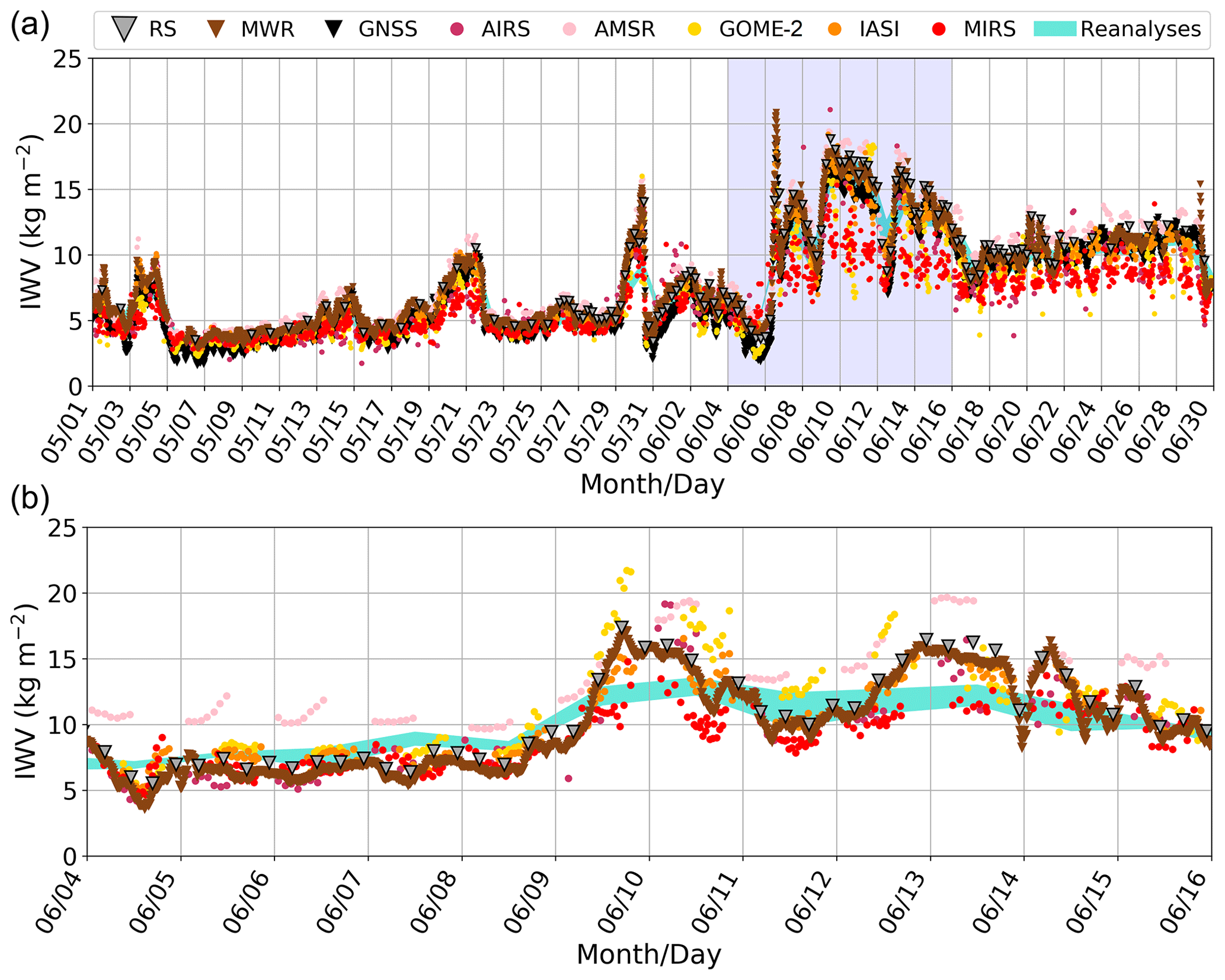
Figure 2 Time series of reference data (GNSS, MWR, radiosonde (RS)), reanalyses and satellites (see legend for explanation of symbols) at the two ACLOUD central sites Ny-Ålesund (a) and the R/V Polarstern ice camp (b). The time period of the ice camp is indicated in blue in the time series for Ny-Ålesund. Note that GNSS is not available for Polarstern. The cyan shaded area indicates the minimum and maximum values of the reanalyses.

Continuous measurements by the MWR and GNSS are able to capture the temporal variability rather well and complement the radiosondes (Fig. 2). Compared to the radiosondes, MWR (GNSS) IWV has a bias of −0.3 (−1.2) kg m⁻² and an RMSD of 0.5 (1.3) kg m⁻² at Ny-Ålesund. Consequently, GNSS is by lower than the MWR by 0.6 kg m⁻², which is also well visible in the time series of 1 individual day (Fig. 4). It is worth noting that these skill scores derived for the ACLOUD period are well in line with those calculated over the period from 2015 to 2018 (not shown), indicating that the biases are rather stable. The SDs between the three different instrument types are lower than 0.8 kg m⁻² and thus make them well suited for the following evaluation of the spatial products.

3 Matching satellite and reanalysis data with reference IWV measurements

All satellites considered have sun-synchronous orbits with orbit durations of about 100 min. For 2017, GOME-2, IASI and MIRS observations are available from the Metop-A and Metop-B satellites, while the AMSR and AIRS are only on board one satellite, reducing their number of samples. Figure 3 illustrates the excellent sampling of the polar orbiters at high latitudes and the complementarity of the morning (Metop) and afternoon (NOAA) orbit, providing nearly continuous sampling over two-thirds of the day. Nevertheless sampling strongly depends on the longitude, and it becomes clear that good matching with the synoptic launch times of radiosondes is often not possible, especially for the eastern regions and the launch time at 00:00 UTC.

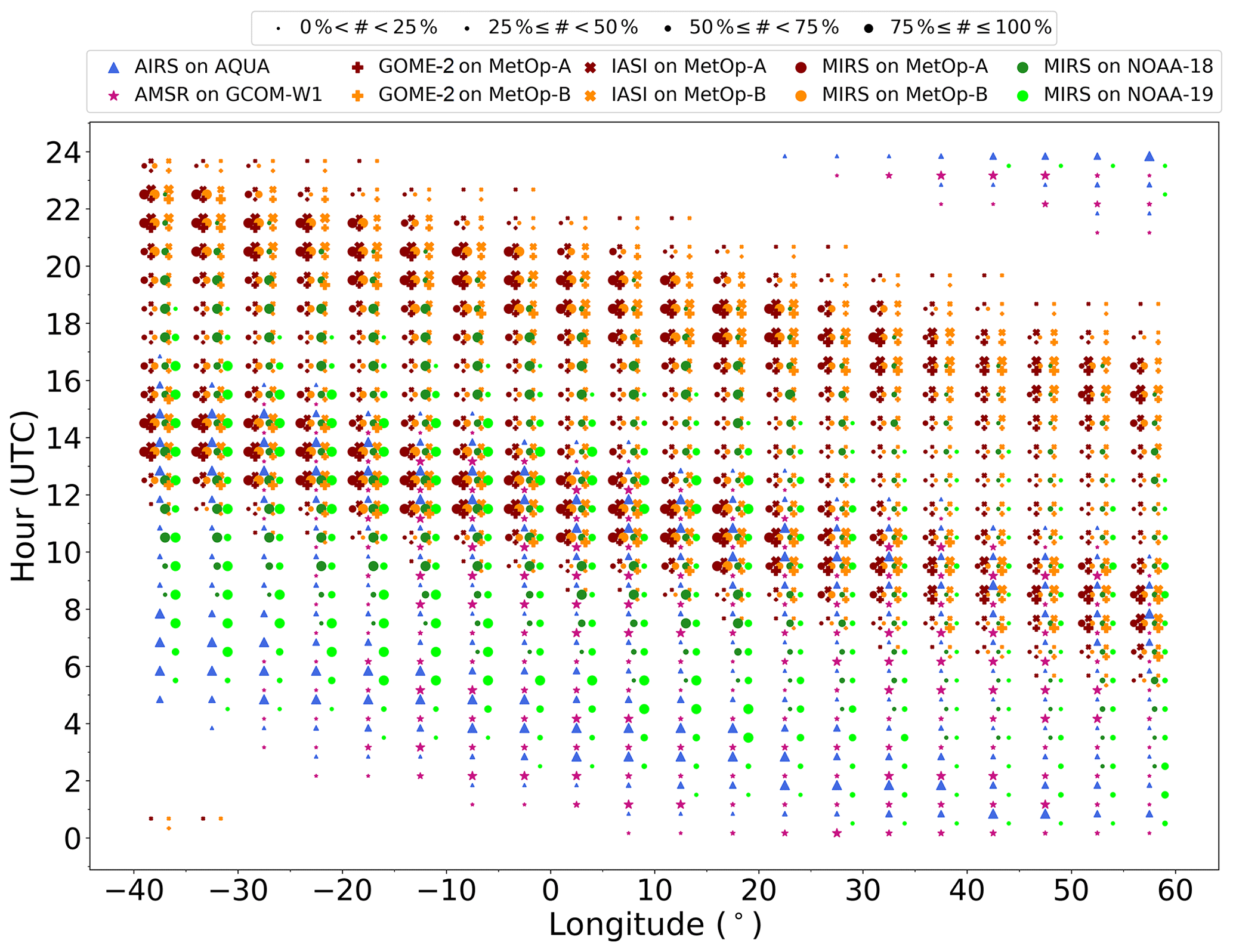
Figure 3 Overview of satellite data sampling for a latitude band (70–80^∘ N) as a function of time of day and longitude (5^∘ resolution). For each bin (1 h, 5^∘) the total number of measurements over the 2-month period (May–June 2017) is indicated per instrument by the size of the corresponding symbol in quantiles. The maximum number of samples per bin is about 2000 for AIRS on Aqua, 8000 for each IASI platform and about 10 000 for the MIRS products on each satellite.

The satellite IWV products were all provided as orbital data on a pixel basis. For the intercomparison with reference data, all pixels with valid IWV retrievals in a radius of 50 km around the individual stations (Fig. 1) were extracted. As an example, Fig. 2 shows the good temporal sampling of satellite and reference (MWR, GNSS, radiosonde) measurements over the full 2-month period for Ny-Ålesund and the 2-week time period for the ice embarkment of the R/V Polarstern close to 81^∘ N. During the shorter period it can be seen that the overpasses by Metop-A and Metop-B, which host GOME-2, the IASI and the MHS, cover the time period between roughly 08:00 and 18:00 UTC rather well for these two reference sites (cf. also Fig. 3), while the AMSR measures in the first half of the day (Fig. 2). The MIRS product covers the widest range as in addition to the Metop satellites also NOAA-18 and NOAA-19 are used.

In order to compare the satellite measurements with reference data, different criteria are used: (i) the highly temporally resolved ground-based MWR data are averaged to 15 min means to match the GNSS measurements. Their temporally closest measurement to the radiosonde synoptic time is used for comparisons. (ii) A time window of ±30 min with respect to the radiosonde time is used to identify corresponding satellite measurements. Note that a larger window length of ±1 h does not drastically enhance the number of matched samples for the radiosondes due to the fixed launch times at most stations. (iii) All IWV satellite measurements with a center pixel location within a 50 km circle around the location of the reference site are used to calculate mean IWV and its SD. The same exercise has been performed for a larger search radius of 100 km to check the sensitivity. (iv) To eliminate outliers, only IWV values between 0 and 30 kg m⁻² are used, which is sensible as IWV varies between 3 and 22 kg m⁻² for the Ny-Ålesund and R/V Polarstern sites (Fig. 2). While we are aware that most satellite retrievals work best over ocean surfaces (well-characterized microwave emissivity) and are affected by differences in orography, we consciously use all conditions for our assessment as we aim at a climatologically sound data set. In order to estimate the influence of orography and surface emissivity, all measurements were classified according to their position over water or land. This is for example of interest for Ny-Ålesund, with a station elevation of 11 m, which is located in a fjord surrounded by mountains up to 550 m height.

For maps of daily and monthly IWV, the reanalysis products were interpolated to the ERA-Interim grid with 0.75^∘ × 0.75^∘ resolution. All orbital satellite data for a day are assigned to the same 0.75^∘ × 0.75^∘ latitude–longitude grid spanning the study area. The daily means are calculated as the arithmetic mean per grid cell, using only measurements which fulfill the quality criteria (Sect. 2.1). Due to the different satellite orbits, sampling differs for the different products (see above). Note that due to the meridian convergence, this means that at 70^∘ N, the resolution along the latitude circle is only 24 km, while it is 83 km in the meridional direction.

4 Results

4.1 Direct comparisons of satellite/reanalysis with reference data

The ACLOUD/PASCAL campaign offers a wide range of IWV conditions to investigate the performance of IWV products. The time series at Ny-Ålesund (Fig. 2) first shows an unusual dry (and cold) phase, followed by an unusual wet (and warm) period (30 May–12 June) connected with high IWV variability, as already described by Knudsen et al. (2018). Afterwards normal conditions prevailed. Further it reveals several IWV peaks (Fig. 2), of which three were identified as ARs following the definition by Gorodetskaya et al. (2014, 2020). ARs are narrow corridors of anomalously high IWV (and integrated vapor transport) typically associated with the pre-cold frontal zone of some (but not all) extra-tropical cyclones. The ARs reaching polar regions stretch from lower latitudes and can gain the majority of their moisture in subtropical latitudes (Terpstra et al., 2021). ARs have also been associated with several cyclones, helping the moisture supply within the same AR structure (Sodemann and Stohl, 2013). In the polar regions ARs are often associated with moisture inversions showing maxima in specific humidity between 800 and 900 hPa (Gorodetskaya et al., 2020). Here we choose the AR event from 6 June 2017 at 12:00 UTC to illustrate the capabilities of the different products (Fig. 4). Note that this is only one out of three AR events that occurred during ACLOUD/PASCAL documented in detail by Viceto et al., (submitted). By definition reanalyses provide information across the full region, revealing the maximum IWV of about 25 kg m⁻² west of Novaya Zemlya, from where an elongated band of IWV stretches westward, passing Svalbard and dissolving north of Iceland with extended cloudiness and convective precipitation. As the data are shown here in their original resolution, differences between reanalyses with respect to gradients, coastal features and maximum IWV are evident, showing the better representation of small-scale features in the high-resolution ERA5 reanalysis.

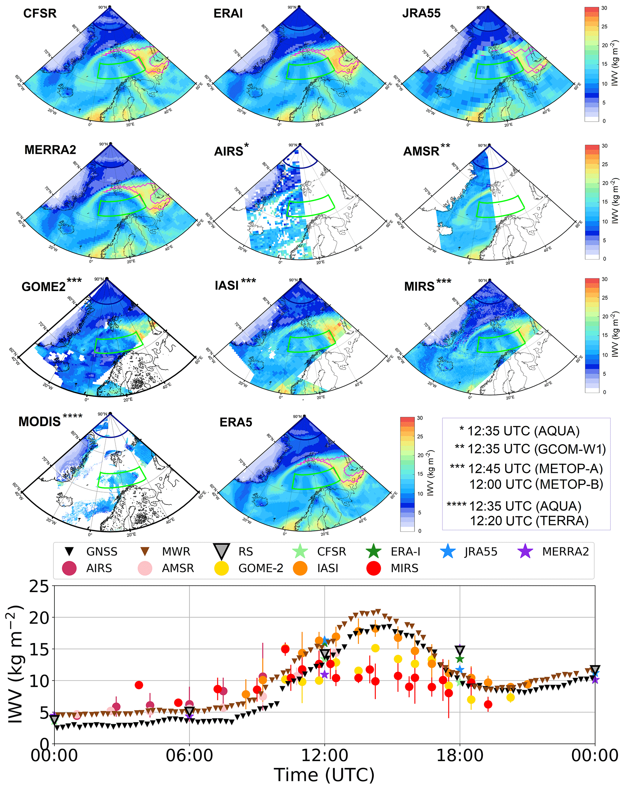
Figure 4 Illustration of the AR event on 6 June 2017 as provided by four different reanalyses at 12:00 UTC and instantaneous satellite measurements (closest orbit in time). The magenta line depicts the region where IWV is higher than an IWV threshold based on the saturated IWV and an AR coefficient (Gorodetskaya et al., 2014) using ERA-Interim reanalysis. For the remaining reanalysis data sets, the line was interpolated from ERA-Interim. The central Arctic (dark blue) and open-ocean (green) regions are marked. Bottom: time series at Ny-Ålesund for 6 June 00:00 UTC to 7 June 00:00 UTC from reference data, reanalyses and satellite measurements within 50 km of the site.

The temporally closest Metop satellite overpass providing GOME, IASI and MIRS products is on the descending branch of the orbit, while Aqua (AIRS) and GCOM-W1 (AMSR) are on an ascending one (Fig. 4). The individual orbits of the satellite products demonstrate the different swath widths as well as the limitations of the products. The AIRS L2 v6 IR-Only product shows the largest spatial gaps due to the limitation of infrared measurements in the presence of clouds and precipitation. AMSR low-frequency microwave information is also available in cloudy regions, but due to the complex emissivity over land only measurements over the ocean and sea ice are provided. GOME-2 provides retrievals over all surfaces, but cloud disturbances lead to data gaps close to Svalbard and north of Iceland. For the latter region, MIRS, which retrieves several parameters simultaneously, indicates precipitation. Note that due to the dominance of the precipitation signal, the information on water vapor can be obscured for heavy rain events. IASI L2 PPFv6 and MIRS, which mitigate cloud influence by the use of microwave radiances in their retrieval schemes, have nearly complete coverage. As already mentioned, MODIS only provides rather limited information as it can derive IWV only under cloud-free conditions over strongly reflective surfaces.

The daily time series of the MWR at Ny-Ålesund (Fig. 4, bottom) shows that IWV rapidly increases by about 15 kg m⁻² within only 5 h, reaching its peak value of 22 kg m⁻² around 14:00 UTC before declining again with similar speed but arriving at a higher level (10 kg m⁻²). The ground-based MWR agrees well with the radiosondes launched during that day, with the exception of 18:00 UTC, which could be caused by the drift of the radiosonde across the strong IWV gradient. GNSS and MWR have a slight mismatch in the diurnal cycle that might be due to the slant path between GNSS satellites and the ground receiver or problems in the derivation of the mean weighted temperature used in the GNSS retrieval (Morland et al., 2009). Generally, it becomes clear that dense temporal and spatial sampling with high resolution is necessary to characterize such an event.

The time series during the AR event (Fig. 4, bottom) reveals differences of up to 6 kg m⁻² at 12:00 UTC between MERRA2 and JRA-55, which is likely due to mismatches in the movement of the AR. Looking at the satellite products shows an even larger spread among the measurements: the AMSR, which has eight overpasses over Ny-Ålesund between 01:00 and 13:00 UTC, agrees very well with the ground-based MWR before the arrival of the AR. During this time also little variability between pixels within the 50 km radius is observed, which increases strongly with the arrival of the AR. IASI L2 PPFv6 provides the best agreement for this case, while GOME-2 and MIRS strongly underestimate the AR maximum. In fact, MIRS seems to have difficulties in retrieving higher IWV values at all, as also indicated in the moist June period (Fig. 2). Consistently with the orbit characteristics of the satellites (Fig. 3), towards the end of the day no satellite matches can be found for Ny-Ålesund.

To quantitatively assess the accuracy of the IWV products, in a first step pairs between radiosonde measurements and corresponding products which fulfill the matching criteria (Sect. 3) are compiled (Fig. 5), and skill scores, i.e., bias, correlation coefficient (r), RMSD and SD (i.e., the bias-corrected RMSD), are computed. For R/V Polarstern (Fig. 5, left column) only few matched samples (between 17 and 32) are available due to the limited deployment time. IASI L2 PPFv6 retrievals can clearly be identified, showing the best performance with the lowest bias (−0.2 kg m⁻²), highest correlation (0.98) and lowest SD (0.9 kg m⁻²). Each individual radiosonde match is an average of about 10 individual pixels, and their low variation indicates relatively homogeneous conditions around the site. This is also seen by the AMSR, which has as well a rather low SD (0.9 kg m⁻²) but is affected by a strong bias (3.2 kg m⁻²).

Figure 5 Scatterplots for radiosondes launched at the Polarstern (left column) and Ny-Ålesund (middle column) and for all other radiosonde stations (right column) with corresponding (±30 min and 50 km radius) satellite measurements (from top to bottom row: AIRS L2 v6 IR-Only, AMSR, GOME-2, IASI L2 PPFv6, MIRS) above all surfaces. All satellite pixels falling into this criterion have been averaged, and their SD is indicated by the width of the line. The number of averaged pixels is indicated by color for the first two columns only.

At Ny-Ålesund (Fig. 5, middle column), where more than twice as many matches are available, the AMSR shows the highest correlation (0.99) and lowest SD (0.7 kg m⁻²) followed by IASI L2 PPFv6 (r=0.97, SD = 1.1 kg m⁻²). Interestingly, the bias of the AMSR is strongly reduced (0.88 kg m⁻²) compared to the ice floe region at R/V Polarstern, indicating an emissivity issue for sea ice. IASI L2 PPFv6 shows a negative bias of −0.7 kg m⁻², which can be explained by the orography around the launch site, as expressed by the reduction in the bias to −0.1 kg m⁻² when only pixels above water are considered. Note that no distinct changes in the other scores occur. The AIRS L2 v6 IR-Only product shows a weaker performance for both sites, with SD being about 0.5 kg m⁻² higher than for IASI L2 PPFv6. This indicates the benefit of the different IASI retrieval strategy, e.g., individual pixels, inclusion of microwave information.

The performance of GOME-2 substantially degrades for IWV values above 10 kg m⁻², leading to much higher SDs at R/V Polarstern (1.6 kg m⁻²) and Ny-Ålesund (1.8 kg m⁻²) than shown by AIRS L2 v6 IR-Only, AMSR and IASI L2 PPFv6. Considering only water surfaces even slightly worsens the scores (not shown). GOME-2 and MIRS show a similar correlation (0.90) for both sites. MIRS, which has the highest number of matches per individual radiosonde, reveals a strong underestimation for IWV values higher than about 10 kg m⁻² for both R/V Polarstern as well as for Ny-Ålesund, where nearly 100 radiosondes are compared. This results in a slope in the regression of 1.44 (1.64) for R/V Polarstern (Ny-Ålesund), which leads to a much narrower retrieved IWV frequency distribution than measured by radiosondes, thus underestimating IWV variability. For MIRS, the scores improve when only water surfaces and a larger search radius (100 km) are used; i.e., correlation increases from 0.90 to 0.95, and SD reduces from 2.3 to 1.6 kg m⁻² (not shown).

When considering all other radiosonde stations together (Fig. 5, right column; Table A1; for locations of stations see Fig. 1), one has to take caution because the different orbit characteristics together with the fixed launch times produce different sets of matched stations for the different products (Fig. 3). Because MIRS makes use of four different satellites, most samples (914) are found. However, MIRS is clearly the product revealing the strongest scatter. This is not necessarily due to the quality of the satellite product but might arise from the consideration of different samples. NOAA-19 has several matches with Russian RS stations, while these are rare for Metop satellites. For Russian RS stations, a slope parameter lower than 1 indicates an overestimation of MIRS, which could be due to problems with surface emissivity, but an underestimation of IWV by the RS can also not be excluded. On the other hand, RS stations in Greenland and northern Scandinavia mainly show slopes larger than 1, indicating an underestimation of MIRS. The use of different radiosonde sensors in different countries or regions is known to result in an uneven distribution of temperature and humidity biases across geopolitical borders (Soden and Lanzante, 1996; Ho et al., 2017; Ingleby, 2017). With a correlation of 0.96, SD of 1.29 kg m⁻² and RMSD of 2.21 kg m⁻², IASI L2 PPFv6 again shows the best performance of all satellite products. While the scatter is much lower than in the case of MIRS, the same trend with respect to over- or underestimation for different stations can be seen. Detailed statistics for all individual radiosonde stations separately are given in the Appendix (Table A1). Note that a direct comparison between the radiosonde measurements and reanalyses has not been pursued as the radiosondes are assimilated into reanalyses.

4.2 Assessment of daily mean data

With the uncertainty in the individual satellite measurements addressed by the direct intercomparison, we now aim to investigate the suitability of the satellite products for climate studies. To better understand how uncertainties are transferred, we first compile daily mean values from orbital data, which are then aggregated to monthly means (cf. Sect. 4.3). Assessing the quality of these products with reference measurements is only possible at sites with continuous ground-based measurements, reducing the data set notably. Therefore, in order to better identify the differences between the products, we look at anomalies with respect to the median of the four classical reanalyses (CFSR, ERA-Interim, JRA55, MERRA2). In case of random noise, a distinct reduction in uncertainty due to averaging should occur, while systematic errors should become more pronounced. In addition, the irregular sampling of satellite data can introduce errors, which will depend on the prevailing weather conditions.

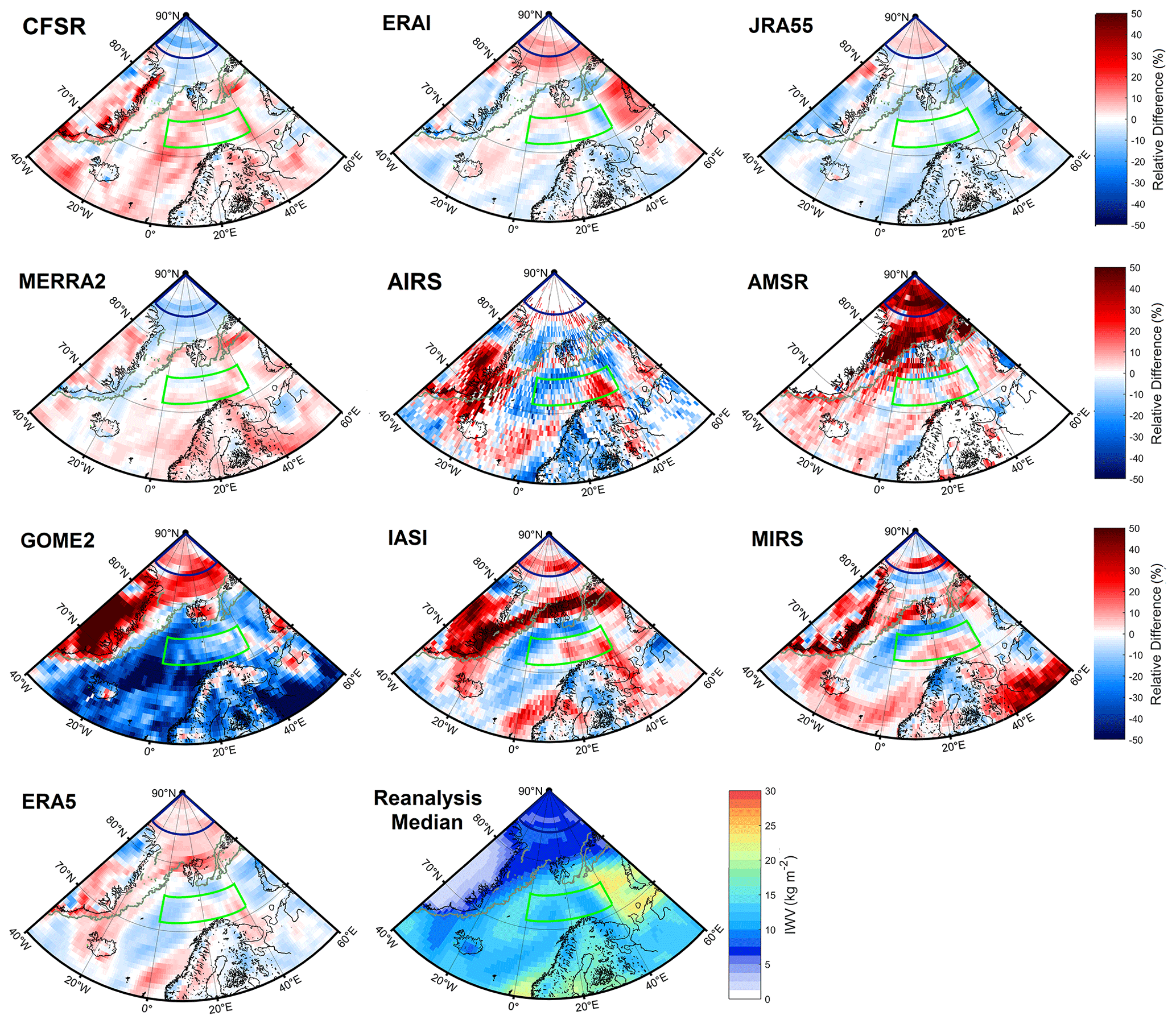
Figure 6 Relative difference in the daily means of the reanalyses and satellite products to the reanalysis median (CFSR, ERA-Interim, JRA-55, MERRA2; lower right plot) for 6 June 2017. The green line indicates the sea ice edge from AMSR sea ice data. The central Arctic (dark blue) and open-ocean (green) regions are marked.

The AR event of 6 June 2017 with high IWV contrasts is used to study the differences between IWV products now on a daily mean basis. Compared to the snapshot at 12:00 UTC (Fig. 4), the AR is smoothed in the reanalysis median over the full day but is still visible (Fig. 6). Differences between reanalyses are around 10 %, with higher deviation along coastlines and strong orography that can easily be explained by differences in their original resolution. In that sense, it is not a surprise that CFSR with its higher resolution shows even higher deviation in some of these areas, e.g., coast of Greenland, as the orography is smoothed less, giving lower IWV at grid points with higher altitude. Over the open ocean, the spatial structure of the differences between the classical reanalyses does not seem to be strongly related to the AR shape, with the exception of the dry line close to 40^∘ E in ERAI, which might hint at differences in the data assimilation of the different reanalyses. Instead already on the daily scale some systematic differences occur over sea ice and the ocean that will be discussed later on. Interestingly, the new high-resolution reanalysis ERA5 (not part of the reanalysis median) substantially differs from the heritage product ERAI, though some similarities such as the positive (moist) difference over sea ice appear.

In general, the deviations of the satellite products from the reanalysis median for 6 June 2017 are about a factor of 2 higher than those of the reanalyses. Different to the reanalyses, the satellite products all have a different sampling density per grid cell due to the different orbit characteristics (Fig. 3). Due to their orbit for these polar-orbiting satellites, the best sampling globally occurs in a band centered around 73^∘ N latitude. AIRS L2 v6 IR-Only and GOME-2 have the lowest number of samples, while IASI L2 PPFv6 and MIRS have around 50 individual measurements per grid cell. In fact IASI L2 PPFv6 and MIRS show very similar geographical structures in their differences, which is no surprise as the IASI L2 PPFv6 product incorporates the microwave measurements on the Metop satellites. The strong bands of positive and negative deviations along the northward extent of the AR, reaching up to 50 % (Fig. 6), can be attributed to sampling differences due to the fast movement of the AR. As the reanalysis median is only computed from the 6-hourly IWV values, the satellites are likely able to better capture this development. This is supported by the similar structures evident in the ERA5 daily mean product (weighting all 1h time steps). The resemblance between ERA5 and the two satellite products (IASI L2 PPFv6 and MIRS) seems to be limited to open-ocean surfaces, where ERA5 assimilates their data. Before we move on to a discussion on systematic effects, we want to investigate the “weather-related” averaging effects in more detail.

During the strong AR event (Fig. 4), clearly high deviations of several kilograms per square meter between different products are possible if the daily mean is calculated from few samples – but how frequently does this occur? To investigate the limitations due to infrequent temporal sampling we use the continuous MWR IWV at Ny-Ålesund, which is available in sub-minute resolution. The basic idea is to mimic the sampling characteristics of other observation systems such as radiosonde stations or sporadic satellite overpasses. During ACLOUD/PASCAL daily mean values calculated from the four time steps such as from 6-hourly radiosonde launches would give a negligible deviation on average with an SD of 0.3 kg m⁻², but individual deviations of 1 kg m⁻² or more occur. When looking at a multiyear data set (2015–2018; not shown), no bias but an SD of 0.5 kg m⁻² is present. Most of the Arctic radiosonde stations launch sondes twice or sometimes only once per day. In this case, the deviations from the true daily mean are even worse. Generally, the SD depends on IWV itself, with a relative SD of 5 % and samples every 6 h, and degrades to 10 % if two samples (00:00 and 12:00 UTC) are used. Taking only the 12:00 UTC measurement as representative of 1 d only slightly worsens the situation, with a relative SD of 12 %.

In the comparison of the daily mean differences, several geographic features appear that point to systematic effects (Fig. 6). Consistent with the previously discussed time series for R/V Polarstern (Fig. 2), the AMSR shows a positive bias over the sea ice of more than 30 %. Over sea ice, also GOME-2 shows a positive bias, pointing at an issue with surface reflectivity for GOME-2 and surface emissivity for the AMSR. The positive bias of GOME-2 over Greenland is partly due to the definition of the product that provides the column above mean sea level. Due to the high elevation of the Greenland ice sheet, the lowest absolute IWV occurs here (see reanalysis median). Therefore small absolute IWV differences lead to high relative differences (also seen by AIRS L2 v6 IR-Only and IASI L2 PPFv6). MIRS shows a high positive overestimation over the Russian land area, consistent with the radiosonde intercomparison.

To better understand systematic features, we study two regions with relatively homogeneous surface conditions over the course of the ACLOUD/PASCAL campaign (cf. Fig. 1). The first region is the high Arctic north of 84^∘ N (in the following called “central Arctic”), where no surface reference measurements exist, and biases between reanalyses are evident: while ERAI and ERA5 show positive deviations over the full sea-ice-covered area, CFSR and MERRA2 show negative deviations as already noted by Rinke et al. (2019). The second area concerns the ice-free North Atlantic towards the Barents Sea (72–75.75^∘ N, 0–40^∘ E; in the following called “open ocean”).

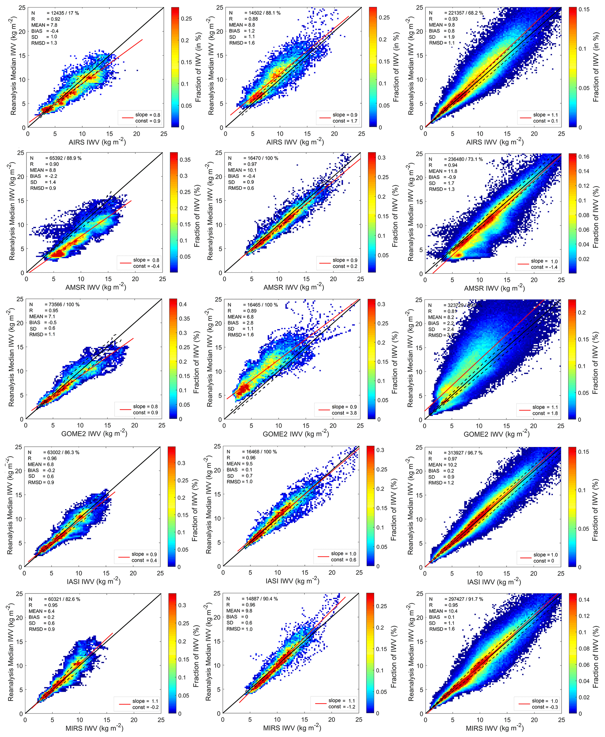
Figure 7 Joint distribution of daily means from the satellite (x axis; AIRS L2 v6 IR-Only, AMSR, GOME-2, IASI L2 PPFv6, MIRS) and reanalysis median (y axis: CFSR, ERA-Interim, JRA-55, MERRA2) for the 0.75^∘ × 0.75^∘ grid points in the central Arctic (left), open ocean (middle) and the full region (right). The time period is May to June 2017. The color indicates the relative fraction of the IWV.

Table 2 Skill scores for the intercomparison of daily IWV mean to reanalysis median in May and June 2017 for all valid data pairs in terms of bias, SD and RMSD (all in kg m⁻²) and correlation coefficient (r). Results have been calculated for the central Arctic, open ocean and the complete study taking into account the area of the different grid cells. N denotes the number of samples.

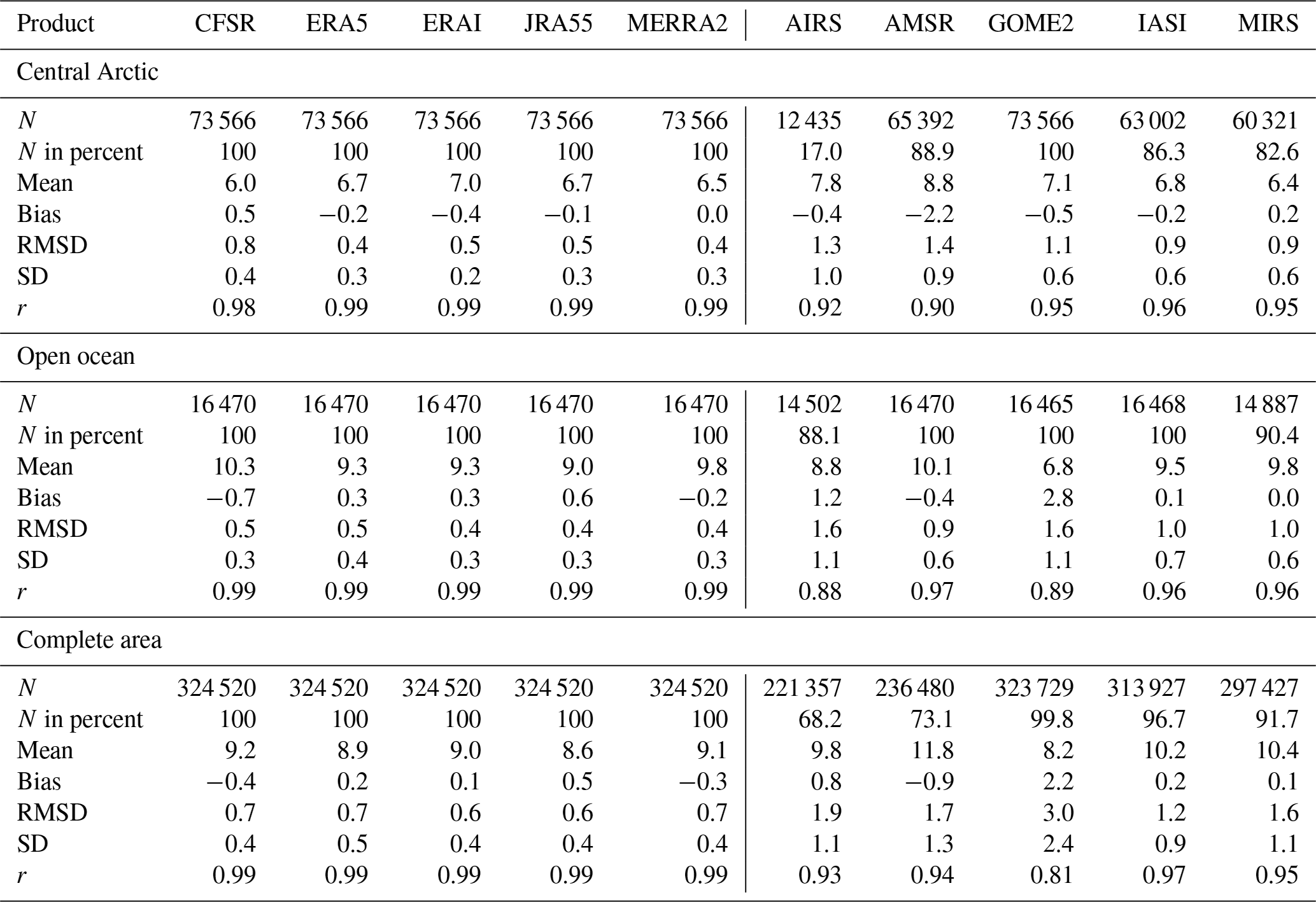
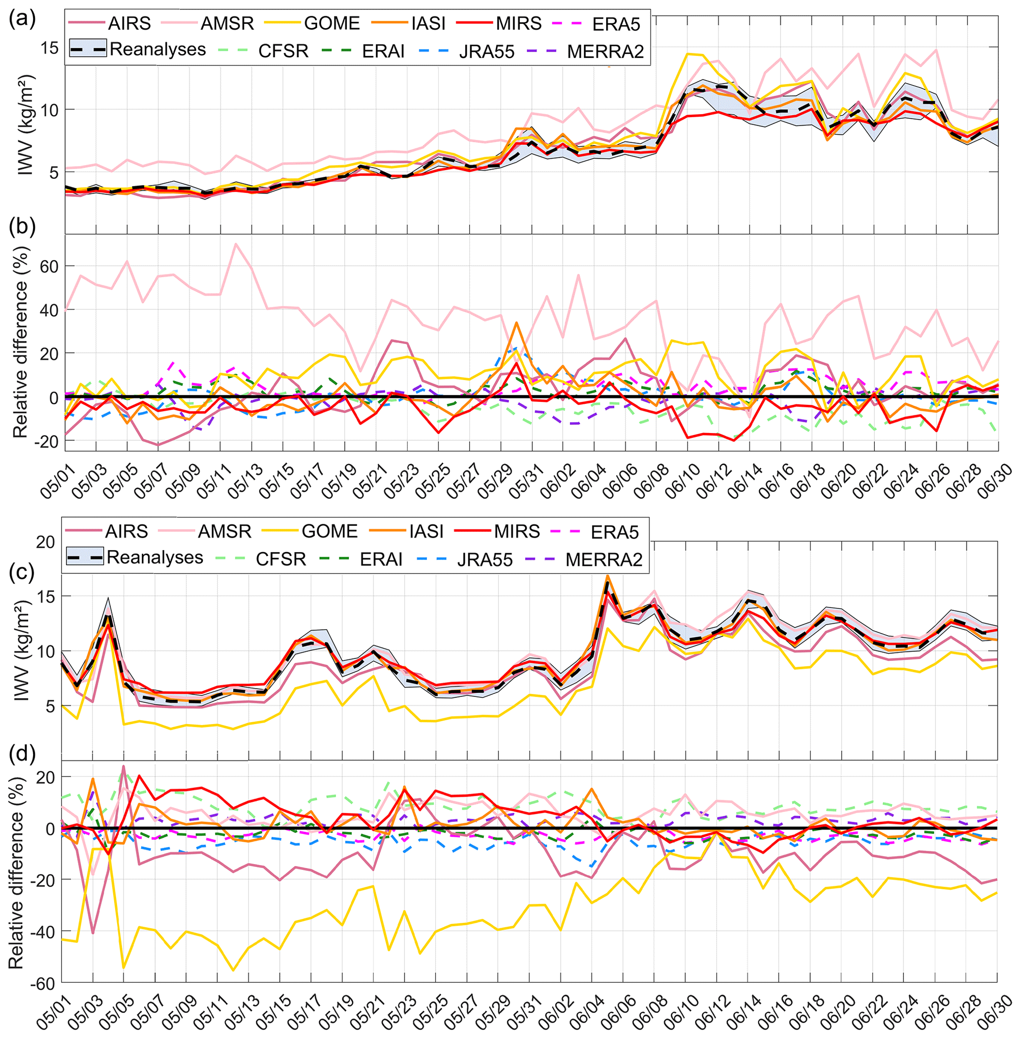
Figure 8 Daily time series of area-averaged IWV for the central Arctic (a, b) and open-ocean (c, d) areas for different products as indicated in the legends. The relative difference is given with respect to the reanalysis median (CFSR, ERAI, JRA55, MERRA2; dashed black line). The shaded area indicates the minimum and maximum values of the reanalyses.

Over the open-ocean area, low-frequency microwave observations should have the best performance due to the low and well-characterized surface emissivity. Therefore it is no surprise that the AMSR shows the lowest SD (0.9 kg m⁻²; Fig. 7, Table 2) compared to the reanalysis median, which might also be due to its assimilation into the reanalyses. The same holds for MIRS and IASI L2 PPFv6 (with SD = 0.6 kg m⁻² and SD = 0.7 kg m⁻², respectively), which incorporate higher microwave frequencies. With frequent low-level cloudiness over the North Atlantic, it is no surprise that the pure thermal IR (AIRS L2 v6 IR-Only; bias = 1.2 kg m⁻², SD = 1.1 kg m⁻²) and solar spectral range (GOME-2; bias = 2.8 kg m⁻², SD = 1.1 kg m⁻²) have difficulties also reflected in the much poorer correlation. The different behavior between the different satellite products is further illustrated by looking at the temporal development over the 2 months (Fig. 8). The AMSR, IASI L2 PPFv6 and MIRS show overall similar performances as the reanalyses, reproducing IWV day-to-day variability well, with daily means between 5 and 15 kg m⁻². In this homogeneous region, reanalyses are highly consistent, with SDs of 0.3 to 0.4 kg m⁻² (Fig. A1). However, the reanalysis bias (Table 2) varies between −0.7 kg m⁻² (CFSR) and +0.6 kg m⁻² (JRA55), which might be related to differences in data assimilation or model physics. In fact, the reanalyses differ in their differences more than the three satellite products, which vary between −0.4 kg m⁻² (AMSR) and +0.1 kg m⁻² (IASI L2 PPFv6). Therefore one might conclude that in open-ocean areas these satellite products can be used to further improve reanalyses.

For the sea ice region, one can nicely see how the rather constant dry conditions in the central Arctic prevailing in the first half of May are changed by moisture transport from the south (Fig. 8). This transport mostly takes place by individual events such as the AR event discussed before that results roughly in a tripling of IWV in the ACLOUD/PASCAL period. The sporadic nature in the transport seems to cause a larger spread between reanalyses and also satellite products (cf. period from 10 June onward). Similar to the open ocean, relative differences between reanalyses are up to ±10 %. Out of the satellite products, only IASI L2 PPFv6 shows similar performance as reanalysis. While GOME-2 showed strong IWV underestimation over the dark open ocean, its performance over the bright sea ice is much more satisfactory, especially at the lower-IWV end. This also becomes visible when time series of area-averaged daily IWV are considered (Fig. 8). As indicated before, the AMSR shows a clear overestimation over the sea ice in the central Arctic and similarly high scattering as AIRS L2 v6 IR-Only. This might also be due to the high sensitivity with respect to the surface emissivity, e.g., leads and polynyas, from which the higher-frequency products (IASI L2 PPFv6, MIRS) are less effected. AIRS L2 v6 IR-Only has only 17 % data coverage as it only flies on one satellite and employs a rigid cloud filtering (Fig. 4)​​​​​​​ so that it is difficult to draw solid conclusions.

For generalizing the results over the full time period (May and June 2017) and full region, all daily mean values are compared with their counterpart from the reanalysis median (Fig. 7, Table 2). While the reanalysis data over the full regions are highly correlated (>0.99; cf. Fig. A1), the correlations reduce for the satellite products. IASI L2 PPFv6 is closest to the reanalyses, with a small bias (0.2 kg m⁻²) and the lowest SD (0.9 kg m⁻²) together with a high coverage of the domain (96.7 %). Interestingly, AIRS L2 v6 IR-Only, which is a pure IR product, performs worse than IASI L2 PPFv6 (bias = 0.8 kg m⁻², SD = 1.9 kg m⁻²) and also shows more data gaps due to a lower spatial coverage and likely also due to cloud filtering. The question is whether these differences are caused solely by the incorporation of microwave measurements into the IASI L2 PPFv6 product or if the incorporation of NWP background data leads to the good agreement with reanalyses.

4.3 Assessment of monthly mean data

For climatological analyses, monthly mean values are typically the shortest timescale considered. Therefore, we further analyze the different monthly means for May (Fig. A2) and June (Fig. 9) 2017 – again in terms of their deviation from the reanalysis median (anomalies). These 2 months are rather interesting as the monthly mean IWV increases roughly by a factor of 2 from May to June, indicating the transition into the Arctic summer. Nevertheless, for all products the anomalies (with respect to the reanalysis median) are rather similar in their geographical patterns for both months. In particular, contrasts between the open ocean, sea ice and Greenland are evident. The AMSR and GOME-2 clearly overestimate IWV over sea ice by more than 20 %. While the AMSR still has slight moist anomalies over the ocean, GOME-2 underestimates here by more than 20 %. A similar pattern (overestimation above sea ice, underestimation over the ocean), albeit with lower magnitude (about 10 %), can be seen for AIRS L2 v6 IR-Only and IASI L2 PPFv6 as well as for the reanalyses ERAI and ERA5. On the other hand, CFSR and to a lesser degree MERRA2 underestimate IWV over sea ice and overestimate over the ocean as well as over Scandinavia and Siberia.

Figure 9 Relative difference between the reanalysis median (bottom right; CFSR, ERA-Interim, JRA-55, MERRA2) and the individual products over the study area for June 2017. The monthly mean sea ice edge for 15 % sea ice concentration derived by the AMSR is shown as a black dash-dotted line. The central Arctic (dark blue) and open-ocean (green) regions are marked.

MIRS shows no major anomaly over ocean areas and just a slight negative difference over sea ice in June. However, in May the sea ice edge close to Svalbard becomes rather prominent, separating the negative (sea ice) and positive (ocean) bias. Particularly striking in MIRS is a strong moist anomaly in the southeastern corner of the study area, where no other products show any spatial anomalies. The positive difference is even stronger in May (>30 %), extending well into Scandinavia. The reason might be that snow melting changes the emissivity in these regions in that season. For completeness, we also consider the MODIS monthly product as this has been used for IWV studies in the Arctic (Alraddawi et al., 2017). MODIS underestimates IWV nearly everywhere except certain oceanic regions. As MODIS can only retrieve over bright surfaces (only sun glint over the ocean), the sampling is rather poor, and small-scale variations occur, which are not evident in the other products.

Table 3 Monthly mean IWV (in kg m⁻²) for May and June 2017 derived for the areal averages of the central Arctic and open ocean. The mean has only been calculated from those grid points which have valid entries for all products. N denotes the percentage of valid grid points in terms of their number and taking the area fraction into account. For Ny-Ålesund (NYA) the closest grid point is shown.

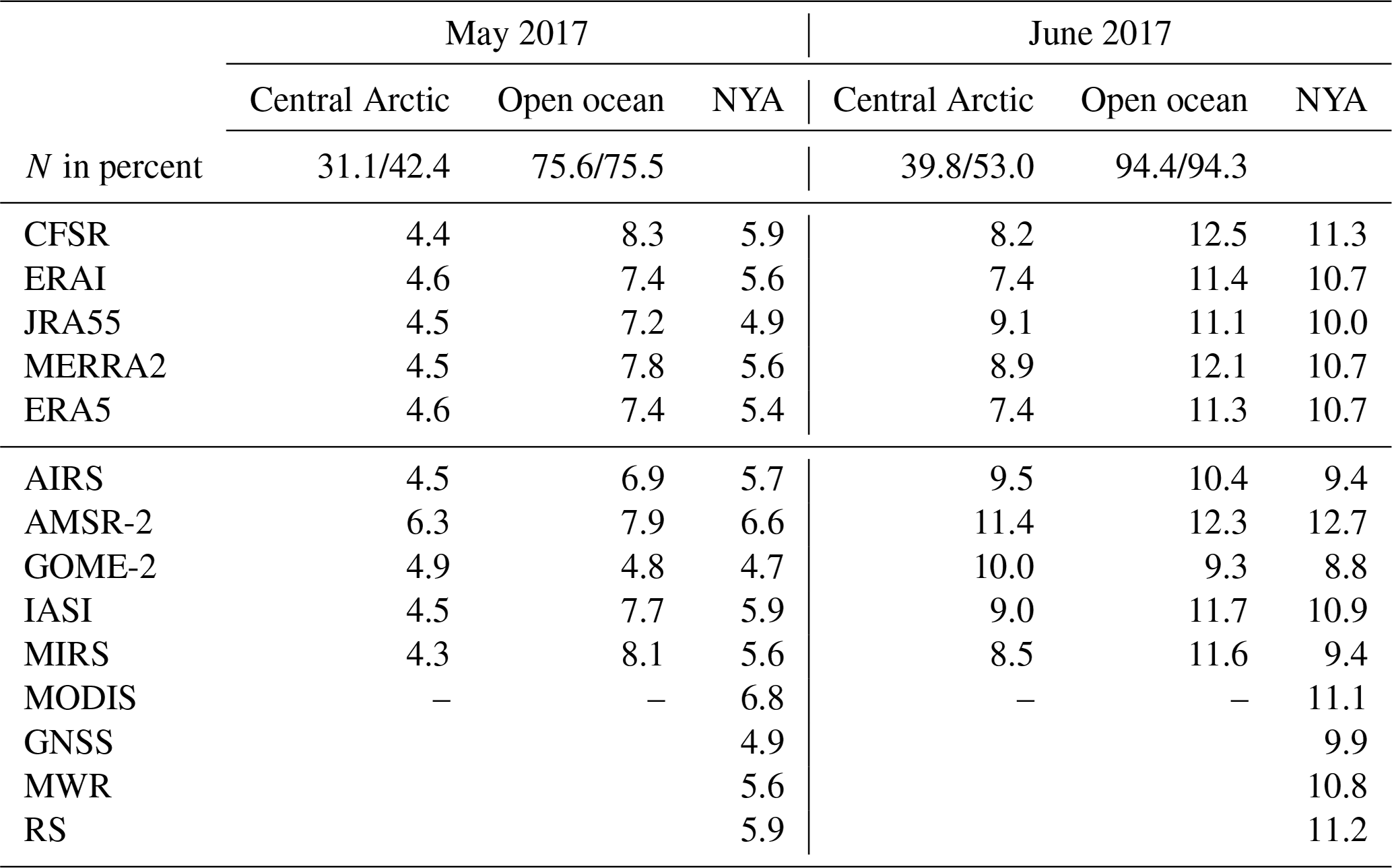
The smooth spatial structures in all products (except MODIS) clearly indicate that weather-related patterns are averaged out on the monthly scale. Biases associated with certain surface types and regions are the dominating uncertainty factors within the different products. To better assess this issue, we compare the mean values of all products for the two selected areas, i.e., the central Arctic and open ocean (cf. Fig. 1), as well as for the closest grid point to Ny-Ålesund (Table 3). During May, when sea ice still persists, reanalyses agree rather well for the central Arctic, with mean values between 4.4 (CFSR) and 4.6 kg m⁻² (ERAI, ERA5). With the exception of the AMSR, satellite products give rather close results, with mean values between 4.3 (MIRS) and 4.9 kg m⁻² (GOME-2). The situation changes for June, when reanalyses have a maximum difference of 1.7 kg m⁻² and satellite products of 2.9 kg m⁻². The reason for this strong difference of about 20 % compared to only 4 % in May is likely to arise from the melting and transformation of the sea ice, affecting air–sea fluxes, and the difficulty to capture the moist intrusions into the Arctic in space and time. For satellite retrievals, the transformation of the sea ice has even stronger consequences as surface reflectivity and emissivity drastically change, leading to differences of about 30 %.

For the open-ocean domain, differences in the IWV monthly means of the reanalyses are around 10 % (slightly higher in May) (Table 3). As already identified by Fig. 8, the AMSR, IASI L2 PPFv6 and MIRS are rather similar as microwave retrievals work best over the open ocean. AIRS L2 v6 IR-Only is not too far off, but the strong underestimation by GOME-2 needs to be better understood and reduced.

Ny-Ålesund with its suite of ground-based instrumentation is well suited to look deeper into the differences in mean IWV. When looking at the ground-based reference data, also differences in their monthly estimates appear. As discussed before, radiosondes have more limitations due to their poorer temporal sampling. Based on the good agreement between MWR and radiosonde data, we consider it for reference here. GNSS underestimates mean IWV by roughly 10 %, but this is still in the range of the reanalyses and satellite products. ERAI and MERRA2 are both very close to the MWR (differences of <0.1 kg m⁻²) in both May and June. From the satellite products, AIRS L2 v6 IR-Only and MIRS agree perfectly with the MWR in May, while IASI L2 PPFv6 is closest in June. This illustrates the difficulty of drawing a solid conclusion on product quality, and certainly longer data records need to be considered.

To put the identified differences into perspective, we analyze how they translate to differences in longwave downward radiation (LWD). Following the approach by Ghatak and Miller (2013), a functional relationship between monthly mean IWV measured by the MWR and LWD as measured by the Baseline Surface Radiation Network station (Maturilli et al., 2015) was derived for Ny-Ålesund (not shown). While there is some scatter mainly arising from different cloudiness in individual months, a clear relation with a nearly linear shape for low IWV saturating for higher IWV values around 15 kg m⁻² is present. According to this relation, the difference in IWV satellite products for Ny-Ålesund of about 1.9 kg m⁻² evident in May relates to a difference of about 20 W m⁻² in LWD, while the stronger IWV difference in June of 2.9 kg m⁻² implies an LWD difference of about 25 W m⁻². This demonstrates the importance of improving the accuracy of estimates at the lower-IWV end.

5 Conclusions and outlook

The role of water vapor in Arctic amplification is still poorly understood partly due to the lack of a solid observational database. Radiosondes launched at only few stations are still considered to be the best climatological record to assess trends, although depending on the used radiosonde type at each station, issues about their uncertainty exist. From their limited data record as well as from global reanalyses, only few regions and seasons with robust IWV trends can be derived (Rinke et al., 2019). With the emergence of new satellite series providing already decade-long data as well as highly resolved reanalysis (ERA5), there is hope for a better assessment of Arctic IWV changes. The ACLOUD/PASCAL period in May/June 2017 performed in the Arctic North Atlantic is exploited to investigate the performance of satellite products as well as reanalyses from instant measurements up to monthly means.

Polar-orbiting satellites provide good sampling at high latitudes such that measurements are typically available every hour, with maximum gaps of 5 h (Fig. 3). Nevertheless, when trying to evaluate satellite products with radiosondes only available at synoptic times, sampling is relatively coarse such that a certain satellite only matches with a limited number of stations. Comparing the performance of different satellite instruments is thus difficult as each instrument “sees” a different set of stations. This gets even more complicated as the quality of radiosondes is likely not comparative across the regions (Ingleby, 2017). For example, there is an indication that stations in the eastern part of the region underestimate IWV, while stations further to the west overestimate. Therefore, in addition to the standard radiosondes, we make use of the high-quality ACLOUD/PASCAL radiosondes launched from the Polarstern frozen into the ice and enhanced launch activity at Ny-Ålesund. For the latter, comparisons over the ocean reveal the best performance by the AMSR (RMSD = 0.6 kg m⁻²), which is not surprising as low-frequency microwave measurements are rather directly related to IWV over the ocean even in cloudy conditions. However, over ice the AMSR shows a pronounced bias. Here, IASI L2 PPFv6 shows the highest skill (RMSD = 0.9 kg m⁻²), which also is true when all radiosonde stations are considered together (RMSD = 1.3 kg m⁻²). The fact that the IASI L2 PPFv6 performance is much better than the one by AIRS L2 v6 IR-Only is attributed on one hand to the utilization of collocated high-frequency microwave observations from the MHS, which enables useful sounding in most cloudy conditions, and on the other hand to differences in the retrieval strategy. MIRS, which depends mainly on MHS measurements, has good coverage as four different satellites are used, but an underestimation of high IWV values is evident at the Polarstern, Ny-Ålesund and radiosonde stations in the northwestern part of the region, while an overestimation for certain Russian stations occurs. Spatial analysis reveals that the overestimation by MIRS (compared to the reanalysis median) extends over a wider region and even far into Scandinavia in May. Therefore this feature could also be related to an insufficient description of the surface, which is undergoing melting of snow at that time of the year.

Water vapor in the Arctic is especially difficult to assess as it is prone to high space and time variability. In case of AR events, changes of more than 100 % can occur within a few hours (Fig. 4). As the reanalyses are mainly anchored by radiosondes in the Arctic, the forecast model becomes important in representing the spatio-temporal development of IWV. This leads to differences of around 10 % in daily mean values (Fig. 6) compared to the reanalyses mean, an effect which is even stronger for the different satellite products due to the less frequent orbits. Nevertheless, we can show that the density of satellite overpasses is high enough for all products – with the exception of MODIS – to smooth out weather-related features within monthly mean IWV.

Overall, in agreement with the radiosonde comparison, the performance by IASI L2 PPFv6 (as judged in comparison to the reanalysis median) is best on the daily as well as on the monthly scale. While a similar AIRS product including other Aqua sensors has been shown to be of similar quality as IASI L2 PPFv6 in the past (Roman et al., 2016), after the failure of Aqua's microwave sensors AIRS L2 v6 IR-Only, using infrared-only measurements displays less accurate IWV than the IASI L2 PPFv6 product. Over the open ocean, the low-frequency microwave product by the AMSR has even slightly less scatter than IASI L2 PPFv6 but shows a slight bias. The bias is much stronger over sea ice in the central Arctic. However, efforts to improve the retrieval with respect to surface emissivity are ongoing. The AMSR is much less affected by clouds than IASI L2 PPFv6 and MIRS, which use the same high-frequency microwave instruments. The better performance by IASI L2 PPFv6 can be explained by the synergistic exploitation of IR and MW. With most clouds being low-level, the hyperspectral IR provides important information on mid-tropospheric moisture, which contributes significantly to IWV in the Arctic, showing frequent humidity inversions. GOME-2 performs well in May over sea ice, but strong overestimation (over Greenland) and underestimation (over the ocean) is apparent.

The reanalysis median was composed of the classical global reanalyses CFSR, ERAI, JRA55 and MERRA2. It is interesting to see that the high-resolution reanalysis ERA5 is not more similar to ERAI than any other reanalyses on the daily scale. However, identifying the reasons behind the differences is not straightforward as changes in the underlying model and in data assimilation can play a role. On the monthly scale, ERAI and ERA5 are rather similar, with positive anomalies over the central Arctic and negative anomalies for the rest of the region, hinting at similar treatment of surface fluxes. In the central Arctic, strong differences of 30 % in IWV monthly means between satellite products occur in the month of June, which likely result from the difficulties of considering the complex and changing surface characteristics of the melting ice within the retrieval algorithms. There is hope that the detailed surface characterization performed as part of the recently finished Multidisciplinary drifting Observatory for the Study of Arctic Climate (MOSAiC) expedition will foster the improvement of future retrieval algorithms.

Appendix A

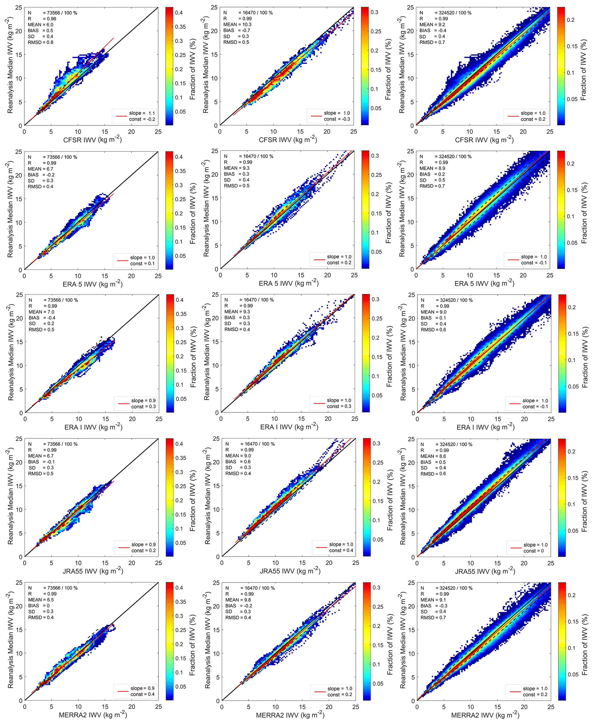
Figure A1 Joint distribution of daily means from the reanalyses (x axis: CFSR, ERA5, ERA-Interim, JRA-55, MERRA2) and reanalysis median (y axis: CFSR, ERA-Interim, JRA-55, MERRA2) for the central Arctic (left), open ocean (middle) and the full region (right). The time period is May to June 2017. The color indicates the relative fraction of the IWV.

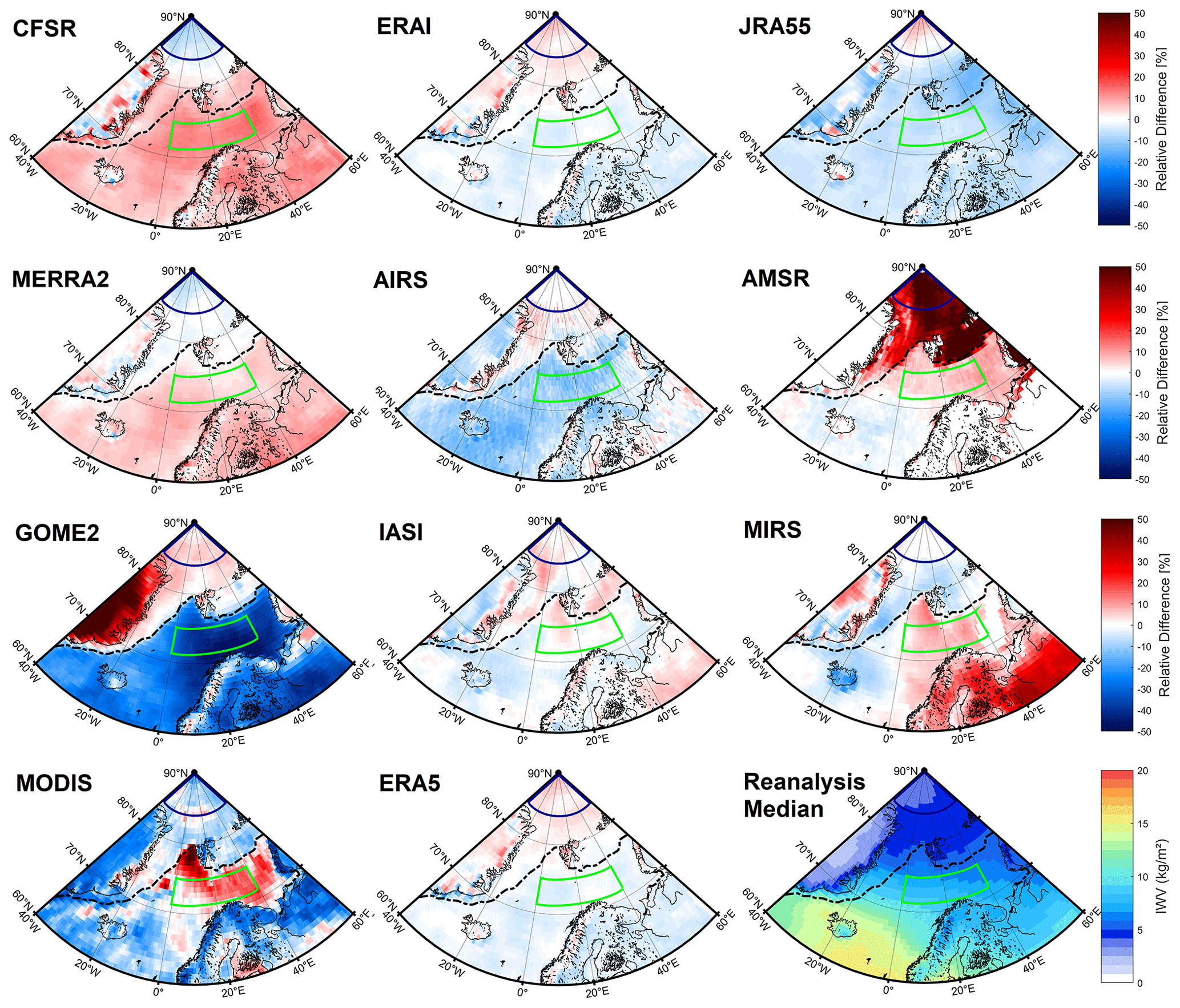
Figure A2 Relative difference between the reanalysis median (bottom right; CFSR, ERA-Interim, JRA-55, MERRA2) and the individual products over the study area for May 2017. The monthly mean sea ice edge for 15 % sea ice concentration derived by the AMSR is shown as a black dash-dotted line.

Table A1 Skill scores for the intercomparison of individual radiosonde stations to satellite IWV in May and June 2017 for all valid data pairs in terms of bias, SD and RMSD (all in kg m⁻²) and correlation coefficient (r). N denotes the number of samples.