Meteor radar observations of polar mesospheric summer echoes over Svalbard

A 31 MHz meteor radar located in Svalbard was used to observe polar mesospheric echoes (PMSEs) during summer 2020. Data from 19 July were selected for detailed analysis, with a focus on extracting additional information to characterize the atmosphere in the PMSE region. The use of an all-sky meteor radar adds an additional use to data collected for meteor observations and enables the detection of PMSE layers across a wide field of view. Comparison with data from a 53.5 MHz narrow-beam mesosphere–stratosphere–troposphere (MST) radar shows good agreement in the morphology of the layer as detected between the two systems. Doppler spectra of PMSE layers reveal fine structure, including regions of enhanced return that move across the radar's field of view. Examination of the relationship between range and Doppler shift of off-zenith portions of the layer enables the estimation of wind speeds with high temporal resolution during PMSE conditions. Trials demonstrate good agreement between wind speeds obtained from PMSE Doppler spectra and those calculated from specular meteor trail radial velocities. Combined with the antenna polar diagram of the radar, this same relationship was used to infer the aspect sensitivity of observed PMSE backscatter, yielding a mean backscatter angular width of $\mathrm{6.8}\pm \mathrm{3.3}{}^{\circ }$. A comparison of underdense meteor radar echo decay times during and outside of PMSE conditions did not demonstrate a strong correlation between the presence of PMSEs and shortened underdense meteor radar echo durations.

1 Introduction

Temperatures in the summer polar mesosphere can fall below the local sublimation point of water vapor, allowing ice crystals to form, particularly when other types of aerosols contribute as condensation nuclei. Larger ice crystals have long been observed as noctilucent clouds (NLCs) at high latitudes (Leslie, 1885). Radar can detect these layers as what Hoppe et al. (1988) coined polar mesospheric summer echoes (PMSEs) (see, e.g., Cho and Röttger, 1997; Rapp and Lübken, 2004). Polar mesospheric clouds (PMCs) in general are of particular interest to atmospheric studies, as they can be a proxy for changes in climate and the impact of solar activity on the middle atmosphere (Thomas, 1996; DeLand et al., 2006). Kirkwood et al. (2002) found that temperature perturbations from 5 d planetary waves may contribute to low temperatures necessary to facilitate PMSEs.

Since the initial detection of PMSEs with VHF (very-high-frequency) radar reported by Czechowsky et al. (1979) at 53.5 MHz and Ecklund and Balsley (1981) at 50 MHz, there have been numerous radar studies of PMSEs (see, e.g., Hocking, 2011). Hoppe et al. (1988) found PMSEs detectable by a 224 MHz incoherent scatter radar, indicating that the Bragg scatter condition is satisfied over a wide range of physical scales. Klekociuk et al. (2008) conducted common-volume measurements in Antarctica of PMCs using lidar and PMSEs using a 55 MHz mesosphere–stratosphere–troposphere (MST) radar, finding 70 % overlap between the different sensors' detections of the two phenomena. Kaifler et al. (2011) presented a similar study in the Northern Hemisphere, including a decade of lidar and MST radar observations of NLCs and PMSEs. Morris et al. (2004, 2006) observed PMSEs using an MST radar in Antarctica, confirming that Southern Hemisphere PMSEs have similar morphology to those seen in the Northern Hemisphere.

There has also been interest in observing PMSEs using meteor radars. These systems are usually comprised of six antennas in total, with a much smaller array footprint than the more sensitive narrow-beam MST radars. Typically used for the determination of winds and temperatures in the 80–100 km region, there is also the possibility of using them for the study of PMSEs. Swarnalingam et al. (2009) used all-sky meteor radars in and around the arctic circle to estimate the effective radar cross section of PMSE scatter. Most recently, Hall et al. (2020) provided an initial report of simultaneous detections of PMSEs by the same narrow-beam MST radar and all-sky meteor radar used in this study.

2 Radars

Data from two radars near Longyearbyen in the Svalbard archipelago (UTC+1) are used in this study to compare observations of PMSE return. An all-sky meteor radar is the primary instrument for exploring new methodologies, and a narrow-beam MST system is used for complementary higher resolution measurements across a restricted field of view and as direct comparison between narrow-beam and all-sky observations.

2.1 NSMR

The Nippon/Norwegian Svalbard Meteor Radar (NSMR) at 78.169^∘ N, 15.994^∘ E is a 31 MHz all-sky interferometric meteor radar transmitting with a peak power of 8 kW. NSMR transmits 3.6 km long 4-bit complementary coded pulses at a pulse repetition frequency (PRF) of 430 Hz and samples at a 1.8 km range resolution. Originally installed in 2001, it was upgraded in December 2019 to use the ATRAD Enhanced Meteor Radar (EMDR) transmitter and digital transceiver (see, e.g., Rao et al., 2014).

NSMR uses a single circularly polarized three-element crossed Yagi transmit antenna and five receive antennas of the same design. Each antenna has a wide central vertical beam with a full-width at half maximum of 81.4–83.6^∘, depending on azimuth, as shown in Fig. 1. The five receive antennas are arranged in a standard Jones cross (Jones et al., 1998), which is comprised of two perpendicular baselines of three antennas spaced at 2 and 2.5 wavelengths from a shared central antenna. The angle of arrival of incident scatter from meteor trails is determined by comparing the phase differences between different antenna pairs (Holdsworth, 2005).

Primary uses of all-sky meteor radar include using meteor detection radial velocities to infer wind speed and direction in the 80–100 km meteor region, as well as using the echo duration of underdense meteors to estimate the local ambipolar diffusion coefficient and, hence, temperature (Hocking, 1999; Cervera and Reid, 2000). More recently, meteor radar has also been used to infer atmospheric density in the mesosphere–lower thermosphere (Younger et al., 2015; Yi et al., 2018)

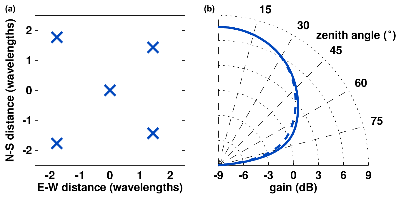
Figure 1 (a) Overhead view of the NSMR receive array, with elements (blue line segments) to scale. (b) Gain pattern as a function of zenith angle for an individual NSMR antenna azimuthally aligned/perpendicular to elements (solid blue line) and 45^∘ between elements (dashed blue line).

Analysis of return from PMSEs was conducted using complex time-series records assembled from in-phase and quadrature components measured for the received signal on each antenna. Reception channels for each antenna were added incoherently to maintain the wide central beam pattern of the individual antennas. While coherent addition of antennas would enhance sensitivity around zenith, the complexity of the sidelobe structure (see, e.g., Fig. 1 of Chau and Clahsen, 2019) makes this unsuitable for the analysis of PMSE Doppler described in Sect. 3.2.

Meteor detection data were characterized using ATRAD analysis software, as described by Holdsworth et al. (2004). Meteor characteristics recorded include range, direction (angle of arrival), radial velocity, echo power, signal-to-noise ratio (SNR), and echo duration.

2.2 SSR

The Svalbard SOUSY Radar (SSR) is a narrow-beam MST radar located at 78.170^∘ N, 15.990^∘ that transmits at 53.5 MHz with a peak power of 8 kW. SSR transmits a 16-bit complementary code at a PRF of 1400 Hz and samples at a 0.5 km range resolution. Based on the mobile SOUSY design (Czechowsky et al., 1984), it has undergone a number of upgrades and changes to configuration (Zecha et al., 2001; Hall et al., 2009), most recently being the installation of a new transmitter and digital transceiver of the same design as NSMR in April 2019. SSR currently uses 356 linearly polarized four-element Yagi antennas to transmit a single 5^∘ full-width at half maximum vertical beam.

Typically, observation time is split between mesospheric and tropospheric observations in 1 min intervals. As with NSMR, complex time-series data were searched for possible PMSE return. It should be noted that results from SSR data are only shown in Fig. 3, with all other results being from NSMR unless otherwise specified.

3 PMSE detection

Following the initial investigation by Hall et al. (2020), NSMR and SSR data for 18–20 July 2020 were analyzed to study PMSE detections in more detail. Weak PMSEs were intermittently detected on 18 July between 06:00–11:00 (all times UTC) and between 07:30–11:30 on 20 July. In addition to the low PMSE signal strength and intermittent occurrence, both these detection periods also displayed significant interference. PMSEs were clearly detected on 19 July, including over 2 h with large signal strength. Data from 19 July are used for illustrative purposes throughout this paper.

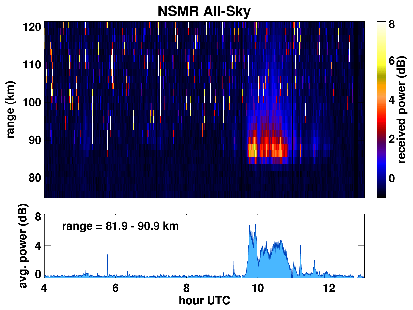
Figure 2 NSMR all-sky received power (incoherently averaged across all five antennas) for 19 July 2020: 30 s averages in 1.8 km range bins. Plot intensity has been capped at 8 dB to enhance the visibility of weak features. The bright vertical segments above 85 km are meteor echoes.

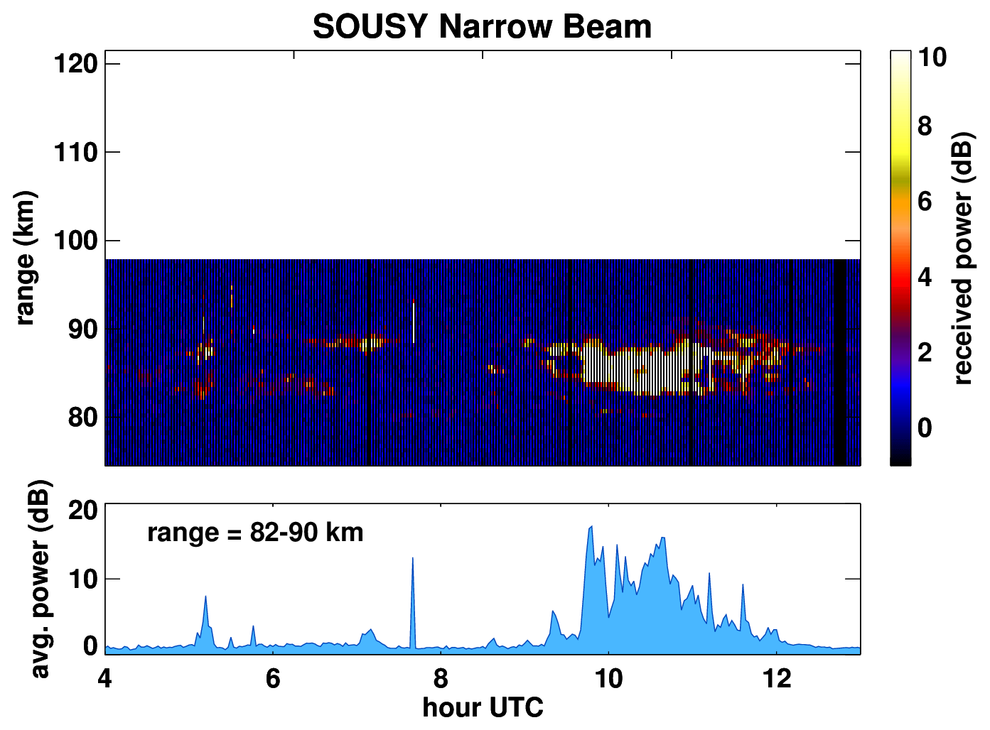
Figure 3 SSR narrow vertical beam received power for 19 July 2020: 1 min averages in 0.5 km range bins. Plot intensity has been capped at 10 dB to enhance the visibility of weak features. Vertical striping is due to interleaving mesospheric observations with other experiments at 1 min intervals.

Detection of PMSEs by NSMR peaked in the 85.5–87.3 km range bin, across different times and with different strengths, as can be seen in Fig. 2. At 05:00–05:30, a small PMSE-like feature was detected. The 1 min Doppler profiles (described in Sect. 3.2) for 06:47–07:38 showed sporadic detections of a very weak PMSE-like feature around 90 km that is not apparent in the range–time intensity plot. A period of strong PMSE detection started at 09:01 and continued until 12:20, with several sub-peaks. The intensity of the main PMSE detection gradually declined from about 11:00, with a low-intensity period seen until around 12:20. PMSE detections by NSMR exhibited vertical smearing on the range–time intensity plot above the primary detection range, which is due to off-zenith detection of the approximately constant height PMSE layer at greater ranges. Strong ionospheric return was also detected by NSMR from 14:10 to 22:45 (not shown).

3.1 Comparison of all-sky and narrow-beam observations

The observations of PMSEs by SSR's narrow vertical beam seen in Fig. 3 strongly correlate with the observations by NSMR. SSR detected the 05:00–05:30 PMSE-like feature more strongly than NSMR and displayed split-layer behavior that was not seen in NSMR data. SSR's detection of the 06:47–07:38 layer was also much stronger than what was seen by NSMR, with two layers clearly visible on the range–time intensity plot. The main PMSE detection by SSR shares a similar time evolution to that seen by NSMR, with transient layer splitting detected between 83–88 km. SSR observations do however exhibit a more gradual decrease from 11:00–12:00, as opposed to the decrease to a low SNR plateau seen by NSMR.

SSR has the advantage of having a 0.5 km range resolution, as opposed to 1.8 km for NSMR. Combined with the focusing of power into a narrower beam, this allows finer details in the PMSE layer to be seen, including split layers and dynamic upper and lower edges. One key difference to NSMR observations is the lack of vertical smearing above the layer, which supports the interpretation that the vertical smearing in NSMR's range–time intensity plot is due to off-zenith detection of a thin layer.

The split layers seen by SSR are consistent, with higher resolution measurements produced by the mobile SOUSY narrow-beam VHF radar (Czechowsky et al., 1989) and the EISCAT VHF incoherent scatter radar (Röttger et al., 1988). The observations of Cho and Röttger (1997) in particular also show periods of split-layer PMSEs, in addition to periods of continuous return across the entire PMSE region. The presence of split PMSE/PMC layers may be further evidence of complex mesopause structures, with multiple distinct local temperature minima (She and Von Zahn, 1998; Thulasiraman and Nee, 2002) allowing for the formation of PMCs at multiple heights.

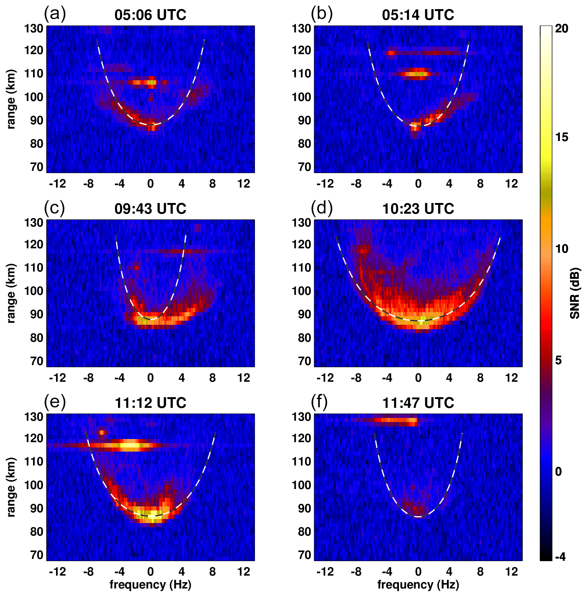
Figure 4 NSMR range–Doppler profiles for 19 July 2020 (0.018 Hz frequency resolution), constructed from 1 min observation periods. (a) Transient PMSE detection. (b) Asymmetric transient PMSEs. (c) Asymmetric onset of strong PMSE return. (d) Strong PMSE return exhibiting fine structure. (e) End of strong PMSE period displaying asymmetric intensity distribution. (f) End of PMSE detection period primarily around zero Doppler. Dashed lines show the expected range–Doppler profile of a thin layer, based on speed calculated from meteor trail detection radial velocities.

3.2 Meteor radar PMSE Doppler profiles

The observation of PMSE layers by a wide field-of-view radar has the advantage that different portions of the horizontal extent of the layer may be detected at differing ranges and Doppler shifts. The curvature of the range–Doppler profile of PMSE detection is related to the speed of the background wind with which the layer is moving. For each Doppler frequency component, the minimum detected range corresponds to return from along the zenith-wind vector plane. Figure 4 shows several examples of Doppler profiles associated with PMSE layers, generated from 1 min long time series. PMSEs are mostly presented in the Doppler profiles as arcs curving upward from the zero-Doppler detection of the layer, the point which corresponds to return from around zenith. The range of PMSE return on the range–Doppler profile at 0 Hz is the height of the layer. Some contamination from meteor echoes is visible in the form of horizontal segments of return in the range–Doppler profile.

The first two profiles from 05:06 and 05:14 are from the weak transient PMSE layer detected by NSMR and SSR. These two profiles differ from the profiles seen for the main detection period in that they exhibit a pronounced asymmetry and an almost linear range–Doppler relation. This may indicate that the scattering geometry for the early transient PMSE detection may differ from that of the main PMSE detection.

The 09:43 profile displays an asymmetric Doppler profile at the onset of strong PMSE return. This is indicative of an anisotropic wind field, as the layer is seen as a region of slow winds (more vertical, negative portion of the profile) which is being replaced as wind speed increases above the radar. At 10:23 there is strong detection during the main PMSE layer period, with fine structure apparent, including layer splitting visible near the edges and multiple small, persistent features. The profile for 11:12 shows the main layer detection as it decreases in amplitude. The mostly negative Doppler asymmetric profile is consistent with the scattering layer leaving the radar's field of view. At 11:47, the PMSE SNR is decreasing towards the end of the detection period, and a significant SNR is limited to around zero Doppler.

3.3 Estimating wind speed from range–Doppler profiles

If it is assumed that PMSEs occur in a thin layer of approximately constant height, then range–Doppler profiles can be used to estimate the wind speed in the PMSE region.

The range R to a point at zenith angle θ and height h above the approximately spherical surface of Earth is given by

$$\begin{array}{}\text{(1)}& {\displaystyle }{\displaystyle }R={\displaystyle \frac{R_{\oplus }+h}{\sin \mathit{\theta }}}\sin \left[\mathit{\theta }-{\sin }^{-\mathrm{1}}\left(R_{\oplus }\sin {\displaystyle \frac{\sin \mathit{\theta }}{R_{\oplus }+h}}\right)\right],\end{array}$$

where R_⊕ is Earth's local radius. Here, the oblateness of Earth is neglected, which is justified on the grounds that PMSEs are detected primarily at zenith angles within $\pm \mathrm{30}{}^{\circ }$ at around 86.4 km (based on zenith angles calculated from Eq. 3 and the extent of observed PMSE Doppler). This means that the horizontal extent of PMSEs detected by meteor radar is not more than 100 km, so there will not be variation in R_⊕ sufficient to significantly affect Eq. (1).

The basic radar Doppler equation for a radar transmitting at frequency f₀ and wind speed V with radial component v_r

$$\begin{array}{}\text{(2)}& {\displaystyle }{\displaystyle }\mathrm{\Delta }f={\displaystyle \frac{\mathrm{2}{f}_{\mathrm{0}}{v}_{\mathrm{r}}}{c-v_{\mathrm{r}}}}\approx {\displaystyle \frac{\mathrm{2}{f}_{\mathrm{0}}{v}_{\mathrm{r}}}{c}}\end{array}$$

can be rearranged, assuming a horizontal wind, to infer the zenith angle of a component of the spectrum with Doppler shift Δf, as

$$\begin{array}{}\text{(3)}& {\displaystyle }{\displaystyle }\mathit{\theta }={\sin }^{-\mathrm{1}}\left({\displaystyle \frac{c\mathrm{\Delta }f}{\mathrm{2}{f}_{\mathrm{0}}V}}\right),\end{array}$$

where c is the speed of light.

Considering the return from the zenith-wind vector plane, it will form a distinct bottom edge to the range–Doppler profile of PMSE return. Therefore, the angular dependence of Eq. (3) can be used to describe the relationship between zenith angle and Doppler shift in the zenith-wind vector plane. Inserting then Eq. (3) into Eq. (1), we have a function $R(\mathrm{\Delta }f,h,V)$, that specifies the curve of the range–Doppler profile of a scattering layer moving horizontally at height h with speed V, resulting in Doppler shifts of Δf.

For NSMR range–Doppler profiles, a least-squares fit was applied to determine the wind speed parameter of $R(\mathrm{\Delta }f,h,V)$ for observation periods where the peak PMSE layer SNR was at least 6 dB. Overall, PMSE-based estimates of wind speed, assuming V is purely horizontal, were mostly in keeping with estimates obtained from the more conventional meteor trail radial velocity technique. This comparison is discussed in further detail in Sect. 4.2.

3.4 PMSE Doppler profile sub-structures

Beyond the range–Doppler relationship due to background winds, the spectra in Fig. 4 also display smaller scale return features that are indicative of scattering from sub-structures within the PMSE layer. The bottom of detected PMSE range–Doppler profiles is generally smooth and in good agreement with the calculated range–Doppler curve for a fixed height, which is indicative of a relatively flat bottom surface of the PMSE layer. The upper bound of PMSE return however exhibits significant variation, including differences in thickness and localized regions of enhanced return. In some cases, it can also be seen that the background wind moves regions of enhanced scatter through the field of view of the radar.

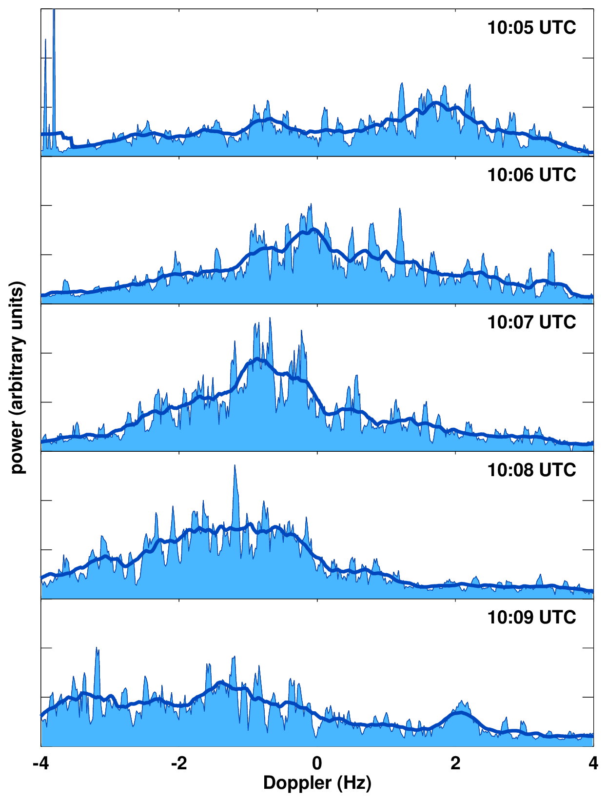
Figure 5 Movement of a perturbation in profiles of the power at the strongest detection range in each frequency bin (0.018 Hz resolution) of PMSE detection for NSMR on 19 July 2020. Solid line is spectral power smoothed with a 0.5 Hz window.

Figure 5 shows the power at the strongest detection range in each frequency bin for 1 min PMSE range–Doppler spectra. In this series of plots, it can be seen that a region of enhanced signal return moves from positive to negative Doppler, changing the shape of spectral power distribution over time. Furthermore, a cursory examination reveals that the speed at which the enhanced return travels from positive to negative Doppler is consistent with the background wind derived from meteor detections and fits to the range–Doppler profile. This demonstrates that the PMSE layer is not homogeneous but contains moving regions of enhanced reflectivity that alter the shape of the spectral power distribution over time.

4 Comparison with meteor detections

The use of a meteor radar to observe PMSEs also presents the opportunity to use conventional meteor radar detections to provide additional information about the state of the atmosphere during and around PMSE detection periods. Meteor radar detections are commonly used to estimate winds in the 80–100 km height range. PMSE-derived wind speeds provide an opportunity to verify the accuracy of meteor-derived wind estimates. Furthermore, PMSEs have been implicated in the anomalously short decay times of underdense meteor echoes below 90 km. The direct detection of PMSEs by meteor radar simplifies the process of assessing the effect of PMSEs on meteor echo decay times, which also relates to the broader study of middle atmosphere plasma chemistry (see, e.g., Rapp and Lübken, 2001; Murray and Plane, 2003, 2005; Friedrich et al., 2011).

4.1 Meteor winds

Winds were estimated in a conventional manner using meteor detection radial velocities to produce wind profiles with 30 min and 2 km vertical resolutions. Meteor-based winds were calculated (assuming the vertical wind w=0) using a least-squares fit to the relation

$$\begin{array}{}\text{(4)}& {\displaystyle }{\displaystyle }{v}_{\mathrm{r}}=ul+vm,\end{array}$$

where v_r is the radial velocity of the meteor trail, u and v are the zonal and meridional components, and l and m are the direction cosines (see, e.g., Holdsworth et al., 2004). Prior to wind estimation, the observed zenith angles θ of meteor detections were converted to local zenith θ_loc angles using the relation

$$\begin{array}{}\text{(5)}& {\displaystyle }{\displaystyle }{\mathit{\theta }}_{\text{loc}}={\sin }^{-\mathrm{1}}\left({\displaystyle \frac{\mathit{\theta }}{R_{\oplus }+h}}\right).\end{array}$$

R_⊕ was calculated at NSMR's latitude using the WGS84 ellipsoid (Decker, 1986).

Outlier rejection was implemented by checking the predicted v_r for each meteor and rejecting any detections differing by more than 30 m s⁻¹. Wind components were then recalculated with the remaining meteors, and the process was repeated until all predicted v_r values were within tolerance. If fewer than six meteors were present in the height/time bin or were left after outlier rejection, it was considered an empty bin.

Seen in Fig. 6, the meteor wind profiles show that the main PMSE detection from 09:01–12:20 coincides with the semi-diurnal tide maximizing the eastward wind just above the layer height and the northward meridional wind maximizing around the layer height.

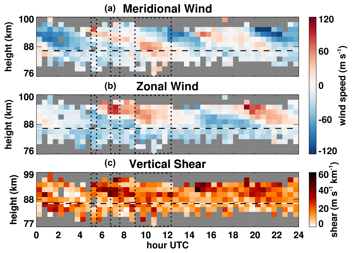
Figure 6 30 min averages of meridional (a) and zonal (b) components of wind and vertical wind shear magnitude (c) calculated from NSMR meteor detection radial velocities in 2 km height bins. The dashed line shows the approximate height (range bin of maximum intensity) of PMSE detection by NSMR. Dotted boxes indicate PMSE detection periods. Gray squares denote insufficient data.

Vertical wind shear was also calculated as the magnitude of the vector difference between winds in adjacent height bins. The main PMSE detection period at 09:01–12:20 occurred during moderate vertical shear (as compared to observed values over the 24 h period), but an examination of the relationship between shear conditions and the occurrence of earlier transient PMSE layers was inconclusive.

4.2 Comparison of meteor and PMSE Doppler winds

In order to compare the observed Doppler profiles of PMSE detections with local wind conditions, winds were estimated using meteor detections for each range–Doppler profile. The wind in the layer region was estimated for each PMSE profile using meteors detected within ±15 min of the profile time and within ±1 km height of the layer's zero-Doppler maximum intensity range.

Seen as dashed lines in Fig. 4, the range–Doppler curves calculated from meteor wind estimates closely match the peak power of the range–Doppler profiles of PMSE return, as seen by the overlap between the dashed lines and PMSE intensity. This is consistent with the interpretation that observed scatter from PMSEs seen by NSMR is from a thin layer as seen across a wide field-of-view. The asymmetric range–Doppler profile for 09:43 shows good agreement for the negative Doppler portion of the spectrum but not the positive Doppler, which is again consistent with a changing wind field in the radar's field of view.

When wind speed estimates from PMSE Doppler and meteor trail radial velocities are directly compared, as shown in Fig. 7, it is seen that the range–Doppler estimates of horizontal wind at the height of maximum PMSE return power are mostly in good agreement with the estimates obtained from meteor trail radial velocities during the main PMSE detection period.

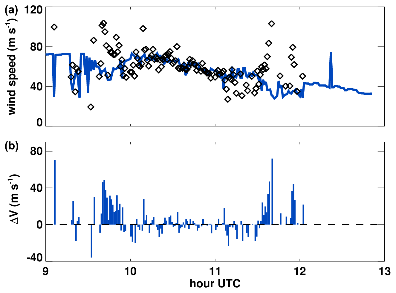
Figure 7 (a) Horizontal wind estimates made using 1 min PMSE range–Doppler fitting (diamonds) and a moving 30 min window of meteor trail detections (solid line). (b) Deviation between meteor and PMSE range–Doppler wind estimates.

Meteor and range–Doppler estimates of horizontal wind speed do not, however, agree at the beginning and end of the primary PMSE detection period for differing reasons at each time. At the beginning of the PMSE detection period, the wind field exhibits significant anisotropy, as evidenced by the asymmetry of the range–Doppler profile at 09:43 in Fig. 4. During this time, horizontal wind speed is increasing with the semi-diurnal tide, resulting in a divergent wind field, with incoming high speed (positive Doppler) winds impinging on a region of slower winds leaving the radar's field of view (negative Doppler). It should however be noted that at NSMR's latitude of 78.169^∘ N, the semidiurnal tide's zonal wavelength is approximately 4095 km. Compared with the horizontal extent of detected PMSEs of about 100 km, this indicates that the observed Doppler asymmetry is not strictly tidal in nature but more likely due to local transient features of the wind field.

A similar reversed situation, albeit with a smaller effect, is seen in the 11:12 example, where the high speed region of the wind field is departing with the incident positive Doppler component displaying a noticeably smaller Doppler. It is also possible that the negative excursion around 09:25 in the meteor wind estimate is due to the same causal factor as the similar negative excursion in the range–Doppler wind speed estimate approximately 10 min later. In this case, it is useful to point out that meteor detections occur across a substantially larger field of view than PMSEs, encompassing a radius of approximately 300 km, as opposed to an approximately 50 km maximum radius for the detected horizontal extent of PMSEs.

As wind speed estimates based on meteor trail radial velocities are dependent on the distribution of meteors within the radar's field of view, there can be times when meteor detections are concentrated more in some parts of the field of view than others. In an anisotropic wind field, this may lead to excess weight being placed on regions of the sky where meteors happen to be detected for a particular observation period. When comparing wind estimates made from the range–Doppler profiles of a thin PMSE scattering layer in a smaller region of the sky with wind estimates made from meteor detections scattered across a larger area, it may be that wind speed estimate perturbations seen by the different methods may be the result of sampling different regions of a divergent wind field.

The disagreement between meteor and range Doppler wind speed estimates at the end of the primary PMSE detection period is due to a different mechanism. From about 11:40–12:00, the significant PMSE SNR in the range–Doppler profile is limited to a narrow spectral region around the zero-Doppler component. Under this condition, the applied fit does not produce an accurate range–Doppler curve. The result is an erroneously flat fit, which corresponds to an overestimate of wind speed. It should be noted that the narrow, flat return at zero Doppler is also indicative of a more aspect sensitive scatter mechanism, wherein detected backscatter is only visible near zenith.

4.3 Meteor echo decay times

The durations of radar echoes from weakly ionized meteor trails, which constitute the overwhelming majority of meteor trail detections, provide information about the state of the background atmosphere in which they occur. The density of plasma in a meteor trail is usually characterized by the “linear electron density”, which is a measure of the radially integrated number of free electrons in a 1 m long segment of meteor trail (along the direction of meteoroid travel).

Underdense meteor trails, with linear electron densities along the trail axis of less than 2.4×10¹⁴ electrons m⁻¹ (McKinley, 1961), produce radar echoes that decay at an exponential rate governed by the local ambipolar diffusion coefficient D (Lovell et al., 1947). The time, τ, for an underdense meteor trail's radar echo to decay to a factor of e⁻¹ of the initial maximum is given by

$$\begin{array}{}\text{(6)}& {\displaystyle }{\displaystyle }\mathit{\tau }={\displaystyle \frac{{\mathit{\lambda }}^{\mathrm{2}}}{\mathrm{16}{\mathit{\pi }}^{\mathrm{2}}D}},\end{array}$$

where λ is the frequency of the radar. This relation is the basis of methods to estimate temperature in the meteor ablation region, either by using the slope of log τ as a function of height (Hocking, 1999) or by supplying pressures to the relation

$$\begin{array}{}\text{(7)}& {\displaystyle }{\displaystyle }D=\mathrm{6.39}\times {\mathrm{10}}^{-\mathrm{2}}{K}_{\mathrm{0}}{\displaystyle \frac{T^{\mathrm{2}}}{p}}=\mathrm{2.23}\times {\mathrm{10}}^{-\mathrm{4}}{K}_{\mathrm{0}}{\displaystyle \frac{T}{\mathit{\rho }}},\end{array}$$

where K₀ is the zero field mobility of the diffusing ions (Mason and McDaniel, 1988), and T, p, and ρ are the atmospheric temperature, pressure, and density, respectively (Cervera and Reid, 2000).

It should be noted that this relation only holds for the case where only ambipolar diffusion is responsible for the evolution of meteor trail plasma. It has been observed that meteors detected at lower altitudes, especially below 85 km, have significantly shorter decay times than is predicted by diffusion alone (Kim et al., 2010). Lee et al. (2013) and Younger et al. (2014) showed that this is most likely due to the neutralization of meteoric plasma initiated by the attachment of free electrons to neutral O₂ and N₂ in a three-body process. It is possible that the ice crystals thought to be responsible for PMSEs also affect the observed decay time of meteor trail echoes, as electrons can attach to ice crystals, leading to additional crystal growth and meteoric plasma neutralization. If this mechanism plays a significant role in meteor trail evolution, then meteor trail decay times should differ in the presence of PMSEs.

Figure 8 Shown are 30 min averages of echo decay times of underdense meteors detected by NSMR in 2 km bins. The dashed line in panel (a) shows the height of the range bin that PMSE return is maximum. Panel (b) shows the 30 min averaged decay time of meteors around the PMSE height. Shaded boxes denote the 95 % confidence interval.

The meteor trail echo decay times seen in Fig. 8 show some correlation between anomalous decay times and PMSE occurrence as minor negative excursions to decay time. The lack of a more dramatic correlation could be due to the dominance of neutral three-body attachment removing free electrons from the trails, as compared to the removal rate due to aerosol attachment to PMC ice crystals. The small negative excursions in decay time coincident with PMSEs around 05:30–06:30 and 09:30–13:00 may be consistent with the findings of Laskar et al. (2019), who estimated an approximately 10 % decrease in meteor decay times in the presence of PMC, although more work is needed to determine if the variation observed by NSMR is due to PMC effects or geophysical variability.

It should be noted that the use of NLC occurrence by Laskar et al. (2019) differs from our use of PMSEs in that PMC/NLC ice crystals are thought to be larger and concentrated at the lower edge of the PMSE region. An examination of NSMR data showed that meteor decay times in lower height bins displayed more temporal stability than meteor detections in the 86–88 km height bin, which suggests that distortion of meteor decay times is not significant at the lower edge of the detected PMSE region. Furthermore, previous work has indicated that the presence of PMCs may actually slow the neutralization of meteor trails by the depletion of mesospheric atomic oxygen (Murray and Plane, 2003). Whatever the precise details of the interaction between PMC particles and meteoric plasma, the presence of detected PMSEs cannot conclusively be proven or ruled out as the primary causal factor in reducing meteor radar echo decay times in this case. An examination of NSMR data across all seasons including a cross-comparison with PMSE detection and non-detection periods is required to definitively answer the question with appropriate statistical rigor.

5 Aspect sensitivity

The detection of Doppler components of the PMSE layer away from zenith presents an opportunity to estimate the angular dependence of observed backscatter from PMSEs. There are however some limitations that the large beamwidth of NSMR imposes on attempts to infer the aspect sensitivity of observed PMSEs. The narrow-beam expression for the aspect sensitivity parameter θ_s as in Hocking et al. (1986) is not applicable in this case, as using Eq. (3) with range–Doppler profiles allows us to directly sample received power within the beam at different zenith angles, rather than tilting the beam. Similarly, the sparse, widely spaced interferometer array makes the use of the Capon method (Sommer et al., 2014) impractical due to the complex beam pattern of the cumulative array. Furthermore, the wide central beam angle of the individual antennas is too large in comparison to the diffraction pattern of individual scatterers to apply spatial correlation analysis (SCA) as in Sommer et al. (2016).

The significant Doppler information available does, however, present an opportunity to gain at least a qualitative description of the aspect sensitivity of PMSEs. As described in Sect. 3.3, the zenith angle of return from a thin layer in the zenith-wind vector plane can be converted to Doppler frequency and vice versa. The return from PMSEs shown in the range–Doppler profiles of Fig. 4 is presented as an arc with a partially filled interior. While return from regions away from the zenith-wind vector plane fills in the interior of the arc, the lower edge of the PMSE return arc corresponds to scatter from within the zenith-wind vector plane.

Hence, the peak powers observed in each frequency bin, which occur at heights that follow an arc closely parallel to the lower range boundary of PMSE return, provide an opportunity to translate observed Doppler shift into an estimate of zenith angle along the wind vector. The peak power at each zenith angle can then be used to infer the angular dependence of PMSE backscatter strength.

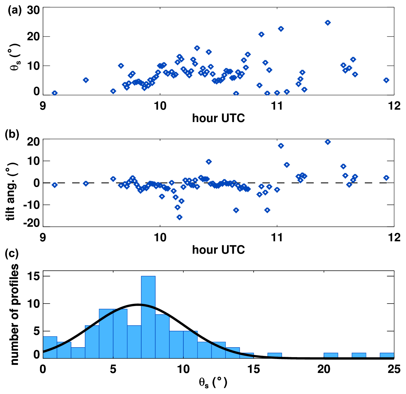
Figure 9 Aspect sensitivity of PMSEs in the zenith-wind vector plane as observed by NSMR. (a) Aspect sensitivity θ_s of PMSE return obtained from Gaussian curve fitted to PMSE Doppler power as a function of Doppler estimated zenith angle. (b) Center of Gaussian curve fitted to PMSE return peak power as a function of Doppler estimated zenith angle. (c) Histogram of PMSE backscatter θ_s estimates. Gaussian fit to the distribution of estimates shown as a solid line.

To do this for each profile, the PMSE range–Doppler estimate of wind speed was applied to Eq. (3) to produce an estimate of zenith angle. The peak power in each zenith angle (frequency) bin was estimated from the amplitude of a Gaussian curve fitted to power in the bin as a function of range. A Gaussian distribution was then fit to the peak powers of PMSE Doppler as a function of estimated zenith angle, corrected for antenna gain. The width of the fitted Gaussian curve is the PMSE aspect sensitivity parameter, θ_s, and the center of the fitted curve is the offset from zenith or tilt angle.

In order to minimize contamination from meteor echoes, zenith-peak power profiles were limited to those with maximum average power less than 600 (arbitrary hardware units). Profiles were also required to have successful Gaussian range and power fits, with peak Doppler SNR between 3 and 30 dB in at least 40 % of zenith angle (frequency) bins. Finally, only Doppler bins in the frequency range of −2.5 to 2.5 Hz were used to exclude the majority of meteor detections that occur with higher Doppler values closer to the horizon.

Applying this process, θ_s was successfully estimated for 76 of the 1 min observation periods between 09:00–13:00. The fitting process additionally provided the offset from zenith, which gives some indication of the preferential scattering or tilt angle of the observed PMSEs. Seen in Fig. 9, ${\mathit{\theta }}_{\mathrm{s}}=\mathrm{6.8}\pm \mathrm{3.3}{}^{\circ }$. The estimated aspect sensitivity showed considerable variation throughout the primary PMSE detection period. The offset of the zenith angle was close to zero with predominantly negative excursions, indicating that the observed PMSEs scattered preferentially in the negative Doppler direction.

The mean and range of estimated aspect sensitivity values seen in Fig. 9 are consistent with other studies (see, e.g., Reid, 1990). For comparison, Czechowsky et al. (1988), exploiting the sidelobes of a radar with similar configuration to SSR at Andenes, found values of 2–10^∘, with typical values in the range of 5–6^∘. Swarnalingam et al. (2011) found a median value of 8–11^∘ using a 51.5 MHz MST radar, with significant dependence on the height of the scattering layer. Larger values were estimated at higher altitudes, which is indicative of increasing isotropy with height. Smirnova et al. (2012), using a 52 MHz MST radar, found two populations of scatterers with aspect sensitivities of 2.9–3.7 and 9–11^∘, also showing an increase with altitude. Both these studies yielded similar results to the earlier work by Huaman and Balsley (1998) that gave mean values of 10^∘ at 80 km and 14^∘ at 90 km but with substantial differences between radars at Andenes (5–6^∘) and Poker Flat (12–13^∘).

This study did not show a clear correlation between layer height and aspect sensitivity. However, it should be noted that the method used is only applicable to the height of maximum scattering intensity, so it does not capture the full behavior of aspect sensitivity in different parts of the PMSE layer.

6 Conclusions

This study demonstrates that all-sky radars provide a useful complement to the more common narrow-beam studies of PMSEs. The key advantage of all-sky systems is that they are able to capture Doppler contributions from PMSEs continuously across a wide range of zenith angles. This reveals fine structure in PMSE layers and provides an immediate opportunity to infer the motion of the scatterers. The use of a 31 MHz radar is also noteworthy, given that most previous radar observations of PMSEs have been conducted with MST radars with transmission frequencies above 50 MHz. This indicates that the $\mathit{\lambda }/\mathrm{2}$ scattering condition is also fulfilled at larger spatial scales than for the more common 50 MHz and above observations. Thus, it has also been shown that the longer wavelength, which is optimized for meteor trail detection, is not a significant impediment to the detection of PMSE layers.

In particular, the range–Doppler profile of thin layer return obtained by wide field-of-view radars can be used to infer wind speed in the layer and the aspect sensitivity of the layer's scattering mechanism. A comparison of wind speeds obtained through this method and more conventional meteor-echo-based wind estimates shows good agreement for fully developed PMSEs, an assessment that is also supported by the apparent motion of density perturbations within the distribution of received power from the layer. Aspect sensitivity estimated using range–Doppler profiles is consistent with previous estimates made using 51–52 MHz narrow-beam MST radars.

While this study was necessarily limited in its scope, the methods presented should in future be applied to longer data sets. Ideally, this will take the form of a campaign over summer at a polar location where frequent PMSEs are observed. Additional data, such as lidar temperatures, could also facilitate a more thorough interpretation of the results of the methods described.