the Creative Commons Attribution 4.0 License.
the Creative Commons Attribution 4.0 License.
 | 28 Jul 2021
Increasing the spatial resolution of cloud property retrievals from Meteosat SEVIRI by use of its high-resolution visible channel: implementation and examples
Carola Barrientos-Velasco
Sebastian Bley
Anja Hünerbein
Stephan Lenk
Andreas Macke
Jan Fokke Meirink
Marion Schroedter-Homscheidt
Fabian Senf
Ping Wang
Frank Werner
Jonas Witthuhn
The modification of an existing cloud property retrieval scheme for the Spinning Enhanced Visible and Infrared Imager (SEVIRI) instrument on board the geostationary Meteosat satellites is described to utilize its high-resolution visible (HRV) channel for increasing the spatial resolution of its physical outputs. This results in products with a nadir spatial resolution of 1×1 km2 compared to the standard 3×3 km2 resolution offered by the narrowband channels. This improvement thus greatly reduces the resolution gap between current geostationary and polar-orbiting meteorological satellite imagers. In the first processing step, cloudiness is determined from the HRV observations by a threshold-based cloud masking algorithm. Subsequently, a linear model that links the 0.6 µm, 0.8 µm, and HRV reflectances provides a physical constraint to incorporate the spatial high-frequency component of the HRV observations into the retrieval of cloud optical depth. The implementation of the method is described, including the ancillary datasets used. It is demonstrated that the omission of high-frequency variations in the cloud-absorbing 1.6 µm channel results in comparatively large uncertainties in the retrieved cloud effective radius, likely due to the mismatch in channel resolutions. A newly developed downscaling scheme for the 1.6 µm reflectance is therefore applied to mitigate the effects of this scale mismatch. Benefits of the increased spatial resolution of the resulting SEVIRI products are demonstrated for three example applications: (i) for a convective cloud field, it is shown that significantly better agreement between the distributions of cloud optical depth retrieved from SEVIRI and from collocated MODIS observations is achieved. (ii) The temporal evolution of cloud properties for a growing convective storm at standard and HRV spatial resolutions are compared, illustrating an improved contrast in growth signatures resulting from the use of the HRV channel. (iii) An example of surface solar irradiance, determined from the retrieved cloud properties, is shown, for which the HRV channel helps to better capture the large spatiotemporal variability induced by convective clouds. These results suggest that incorporating the HRV channel into the retrieval has potential for improving Meteosat-based cloud products for several application domains.
- Article
(5943 KB) - Full-text XML
- Companion paper
- BibTeX
- EndNote


Clouds play an important role in Earth's energy budget and hydrological cycle (e.g., Wild and Liepert, 2010). Despite their importance, the representation of clouds in current climate and weather forecast models remains limited due to a fundamental lack of understanding of the relevant cloud processes and the interaction of clouds with other components of the climate system (Bony et al., 2015). These shortcomings are widely recognized to be a dominant source of uncertainty in our understanding of the climate system and its response to anthropogenic forcings (Boucher et al., 2013).
Due to their excellent spatial and temporal coverage, as well as the multi-decadal length of observational data records, multi-spectral meteorological satellite imagers offer a unique source of information for studying the role of clouds in the climate system. The underlying methods for inferring cloud properties from these instruments are, however, usually nonlinear and sensitive to assumptions and uncertainties in the applied forward models, which reflects the underconstrained nature of the underlying inversion problem (Stephens and Kummerow, 2007). This introduces sensitivities of the resulting products to sensor characteristics, such as spectral response and spatial resolution, as well as relatively minor differences in the implementation of retrieval algorithms (Roebeling et al., 2015). As a result, inhomogeneities and inconsistencies can be found in cloud data records from different satellite platforms or data providers (e.g., Karlsson and Devasthale, 2018).
Currently, the Moderate Resolution Imaging Spectroradiometer (MODIS) flown on the polar-orbiting satellites Terra and Aqua is one of the most widely used satellite instruments for studying the role of clouds in the climate1. A subset of the MODIS cloud products is based on solar reflectances and the bi-spectral method described by Nakajima and King (1990) (e.g., estimates of cloud optical depth, effective radius, and water path) at a spatial resolution of km2 (Platnick et al., 2003, 2017).
Despite their wide use, it is well-recognized that sub-pixel variability and 3D radiative effects can cause retrieval failures (Cho et al., 2015) or introduce substantial biases and uncertainties in these products, which depend on various factors such as solar and viewing geometry (see e.g., Cahalan et al., 1994; Marshak et al., 2006; Zhang et al., 2012; Horváth et al., 2014). While the cloud droplet number concentration is of high scientific interest due to its relevance for elucidating the climate impact of aerosol–cloud interactions, its estimation from bi-spectral solar reflectances by means of cloud optical depth and effective radius (see e.g., Quaas et al., 2006) is particularly sensitive to such uncertainties (Grosvenor et al., 2018).
In contrast to polar-orbiting satellites, observations from a geostationary orbit allow for fully resolving the diurnal cycle (e.g., Seethala et al., 2018) and studying the temporal evolution of shallow and deep convective clouds (e.g., Bley et al., 2016; Senf et al., 2015). They are also widely used to derive surface solar irradiance (SSI) as needed by the solar energy community (e.g., Tarpley, 1979; Möser and Raschke, 1984; Cano et al., 1986; Rigollier et al., 2004; Greuell et al., 2013; Qu et al., 2017).
While the recently launched geostationary Himawari and GOES-R series satellites carry instruments with a similar spectral response and spatial resolution as MODIS for their solar channels (Miller et al., 2016; Schmit et al., 2017), such observations are not yet available over Europe, where the third generation of Meteosat with similar spatial resolution capabilities is scheduled for launch in 2022. The current operational second-generation Meteosat satellites are equipped with the Spinning Enhanced Visible and Infrared Imager (SEVIRI) instrument, with a presently comparatively coarse nadir spatial resolution of 3×3 km2 for its narrowband spectral channels (Schmetz et al., 2002). Considering the start of SEVIRI's operational service in 2004 and thus the length of its observational record, as well as its relatively advanced sensor characteristics, SEVIRI data remain of high interest for both scientific investigations in atmospheric and climate sciences and for usage by solar energy industries.
In addition to its 11 narrowband channels, the SEVIRI instrument features a high-resolution visible (HRV) channel with a nadir resolution of 1×1 km2. The HRV channel is widely used to derive SSI with cloud-index-based methods (e.g., Rigollier et al., 2004, as used in Helioclim-3, see http://www.soda-pro.com/de/help/helioclim/helioclim-3-overview, last access: 3 August 2020; Hammer et al., 2003, as used in EnMetSol, see https://uol.de/en/energiemeteorology/services/enmetsol, last access: 3 August 2020; or Pfeifroth et al., 2019). Despite some previous studies (e.g., Klüser et al., 2008; Carbajal Henken et al., 2011), a systematic and quantitative use of the HRV channel for producing cloud property datasets based on physical retrievals has not been pursued. The present article aims to fill this gap by extending and combining the methods introduced in Deneke and Roebeling (2010) and Bley and Deneke (2013), as well as introducing techniques for utilizing the HRV channel together with SEVIRI's other channels for quantitative cloud retrievals. This effort builds on the well-established cloud physical property (CPP) retrieval described by Roebeling et al. (2006), which is also utilized at the heart of the CLAAS-1 and CLAAS-2 climate data records (Stengel et al., 2014; Benas et al., 2017) provided by the Climate Monitoring Satellite Application Facility (CM SAF; Schulz et al., 2009).
By applying the Surface Irradiance for Cloudy Conditions from SEVIRI (SICCS) algorithm (Deneke et al., 2008; Greuell et al., 2013) to the improved cloud properties at HRV resolution, corresponding solar irradiances at the surface and the top of the atmosphere (TOA) can also be retrieved with this scheme. The simultaneous and consistent retrieval of cloud properties and irradiances can help to answer the question of whether higher spatial resolution of satellite observations can improve the agreement with ground-based cloud and irradiance measurements. It may also help to quantify which accuracy can be achieved for different types of clouds and which physical mechanisms are responsible for deviations.
The present paper is a companion paper to Werner and Deneke (2020), which focuses on the methodological choices and details of the downscaling algorithm for the SEVIRI reflectances and presents an evaluation of the accuracy of the retrieved cloud products using MODIS observations as a reference. In contrast, the present paper gives an overview of the complete retrieval setup, including its ancillary inputs, and describes three applications which might potentially benefit from the enhanced resolution.
The paper is structured as follows: in Sect. 2, the relevant instrumental characteristics of Meteosat SEVIRI used as a basis of this paper are introduced. Sect. 3 summarizes the various steps in the overall processing scheme. Special attention is given to describing the modifications required to utilize the HRV channel. Sect. 4 presents some example applications and illustrates the benefits resulting from the increased spatial resolution. Sect. 5 closes by drawing conclusions and presenting an outlook to future work.
Meteosat Second Generation is the current series of European geostationary weather satellites operated by the European Organisation for the Exploitation of Meteorological Satellites (EUMETSAT). Four MSG satellites have been launched since 2003 and carry SEVIRI as a main payload (Schmetz et al., 2002). While the primary objective of MSG is to acquire full-disk imagery for meteorological applications at 0∘ longitude with a 15 min repeat cycle, the backup satellites have provided the so-called Rapid Scan Service (RSS) since 2008, which covers Europe with an enhanced 5 min repeat cycle at a nominal sub-satellite longitude of 9.5∘E.
The SEVIRI instrument has three solar and eight infrared narrowband spectral channels with a nadir sampling resolution of 3×3 km2. In addition, the high-resolution visible (HRV) channel offers an increased spatial resolution of 1×1 km2 at nadir, but at the cost of a relatively broad spectral response resembling that of the first generation of Meteosat satellites (Cros et al., 2006). A further limitation is the fact that HRV images are only available for half of the nominal field of view of the narrowband channels due to its high data volume.
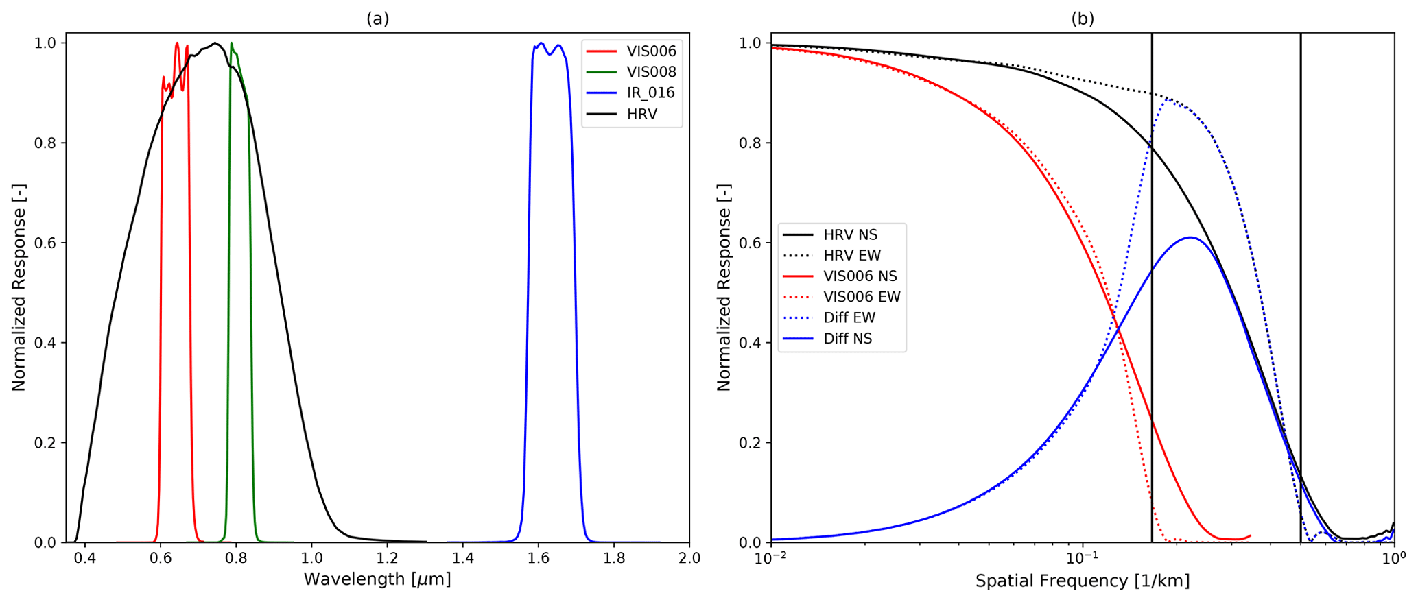
Figure 1Normalized spectral response of the solar channels of the Meteosat SEVIRI instrument (a). The red, green, blue, and black lines correspond to the 0.6 µm (VIS006), 0.8 µm (VIS008), 1.6 µm (IR_016), and HRV channels, respectively. (b) The modulation transfer function of the HRV (black) and the 0.6 µm (red) channels in the north–south (NS, solid) and east–west (EW, dotted) directions. The vertical black lines show the Nyquist frequency limit of the respective channels depending on their sampling resolution. The differences (Diff) of the two modulation transfer functions in both directions are shown in blue (adapted from Deneke and Roebeling, 2010).
Figure 1 shows the spectral response of the solar channels in panel (a), while the modulation transfer function (MTF) in the north–south and east–west direction (as provided by EUMETSAT, 2012) is displayed in panel (b). The vertical black lines correspond to the Nyquist frequencies for the sampling resolution of the respective channels. The MTF describes the attenuation of the amplitude of a sine-like pattern as a function of frequency and is linked to the spatial response through the Fourier transform (see Deneke and Roebeling, 2010, for details). The difference in the MTFs of the HRV and the 0.6 µm channel is also plotted in the figure. It is used in our method to extract the high-spatial-frequency component contained in the HRV channel observations, which is not resolved by the lower-resolution channels, as is described in detail in Sect. 3.5 of the paper. The combination of this high-frequency component with the narrowband channels relies on a sufficiently accurate channel co-registration. For the solar channels, the co-registration accuracy is specified to be better than 0.6 km by EUMETSAT (Schmetz et al., 2002). The results of Deneke and Roebeling (2010) suggest that the true accuracy is in fact significantly better, with a systematic and random magnitude of about 0.1 and 0.3 km, respectively, and effects of misalignment are neglected here. It should also be noted that the optical resolution of the SEVIRI channels is lower than their sampling resolution by a factor of about 1.6, which can be seen by the significant attenuation of the frequency response well below the Nyquist limit. This causes oversampling and implies a significant increase in the effective area sampled by each pixel compared to the area calculated from the sampling resolution (Schmetz et al., 2002).
Moreover, for higher-latitude regions the spatial resolution is also reduced due to the oblique viewing angle of Meteosat, resulting in an increase in the pixel extent by roughly a factor of 2 in the north–south direction for observations over Germany.
EUMETSAT provides an operational calibration of SEVIRI images obtained by a vicarious calibration technique (Govaerts et al., 2004). Comparing collocated near-nadir reflectances from the SEVIRI and MODIS instruments and accounting for differences in spectral response between the instruments, Meirink et al. (2013) confirm the temporal stability of this calibration but find relatively large systematic differences of up to 8 %. Channel-specific correction factors to account for these differences have been derived and are applied by the CM SAF for generating SEVIRI-based climate datasets (e.g., Benas et al., 2017) based on the expectation of the authors that the MODIS calibration is more reliable. Here, the decision has been made to also adopt the same correction factors for the retrievals within the scope of the present study.
The primary objective of the Meteosat satellites is to support short-range weather forecasting in general and forecasting of rapidly developing high-impact weather events in particular. In addition, its observations are currently used in a wide range of applications in meteorology, hydrology, and climatology. Among these, the monitoring and nowcasting of surface solar irradiance for estimating photovoltaic or solar thermal power yield is a growing field of relevance for the transition to renewable energy.
This section presents a description of the improved processing scheme, which has been established for retrieving cloud products and solar irradiance at the TOA and surface from Meteosat SEVIRI at HRV resolution.
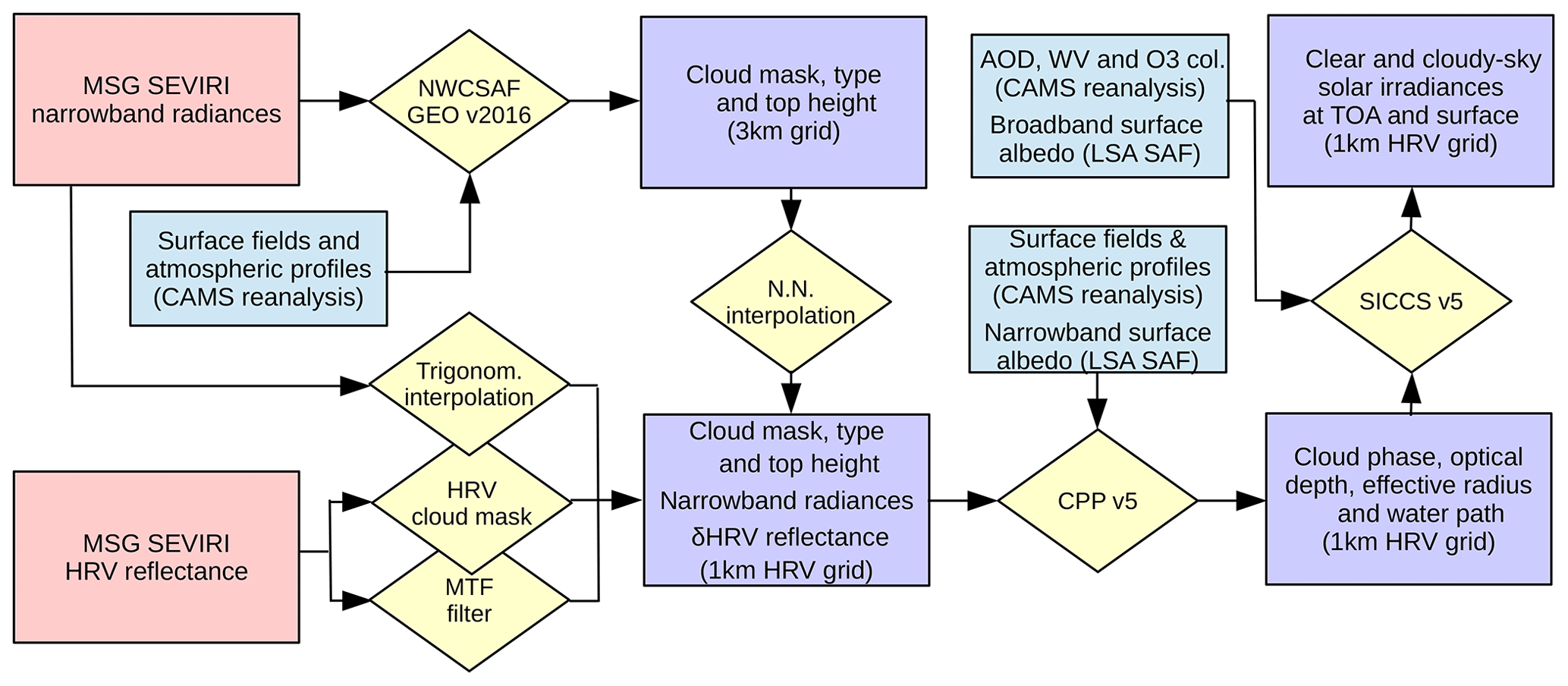
Figure 2Illustration of the workflow of the improved cloud property retrieval scheme based on observations from the Meteosat SEVIRI instrument at its HRV channel resolution. See Sect. 3 for acronym definitions and further explanation.
An overview of the overall workflow is given in Fig. 2. This scheme builds upon software packages developed within the framework of the Satellite Application Facility on Support to Nowcasting and Very Short Range Forecasting (NWC SAF; Fernandez et al., 1999) and on Climate Monitoring (CM SAF; Schulz et al., 2009). While the former software is utilized in unmodified form, the latter CPP code (Roebeling et al., 2006) has been adapted to work on input data interpolated to the grid of the HRV channel and to exploit the additional information content on high-frequency spatial variability captured by the HRV channel, which is not resolved by the lower-resolution narrowband channels. For this purpose, the HRV channel reflectances are filtered by a high-pass filter, thereby removing the variability already resolved by the lower-resolution narrowband channels, and are then used as additional inputs. Also, the normal CPP input fields consisting of SEVIRI level 1.5 radiances and the NWC SAF cloud mask, type, and height products, as well as the ancillary data, are interpolated to the spatial grid of the HRV channel. Consistent with Deneke and Roebeling (2010), trigonometric interpolation is used for the radiances, while nearest-neighbor (NN) interpolation is used for the cloud products and bilinear interpolation for the ancillary datasets. In addition, a high-resolution cloud masking algorithm is applied to the HRV channel reflectances, which has been introduced previously by Bley and Deneke (2013), and is used to improve the standard-resolution NWC SAF cloud mask in particular with respect to the occurrence of small convective clouds, as is described in Sect. 3.5. In the final step of the processing chain, these cloud products are used in combination with ancillary data on surface albedo, water vapor, and ozone column values by the Surface Insolation under Clear and Cloudy skies derived from SEVIRI imagery scheme (SICCS; Deneke et al., 2008; Greuell et al., 2013) to obtain estimates of the clear-sky and cloudy-sky solar irradiances at the TOA and the bottom of the atmosphere.
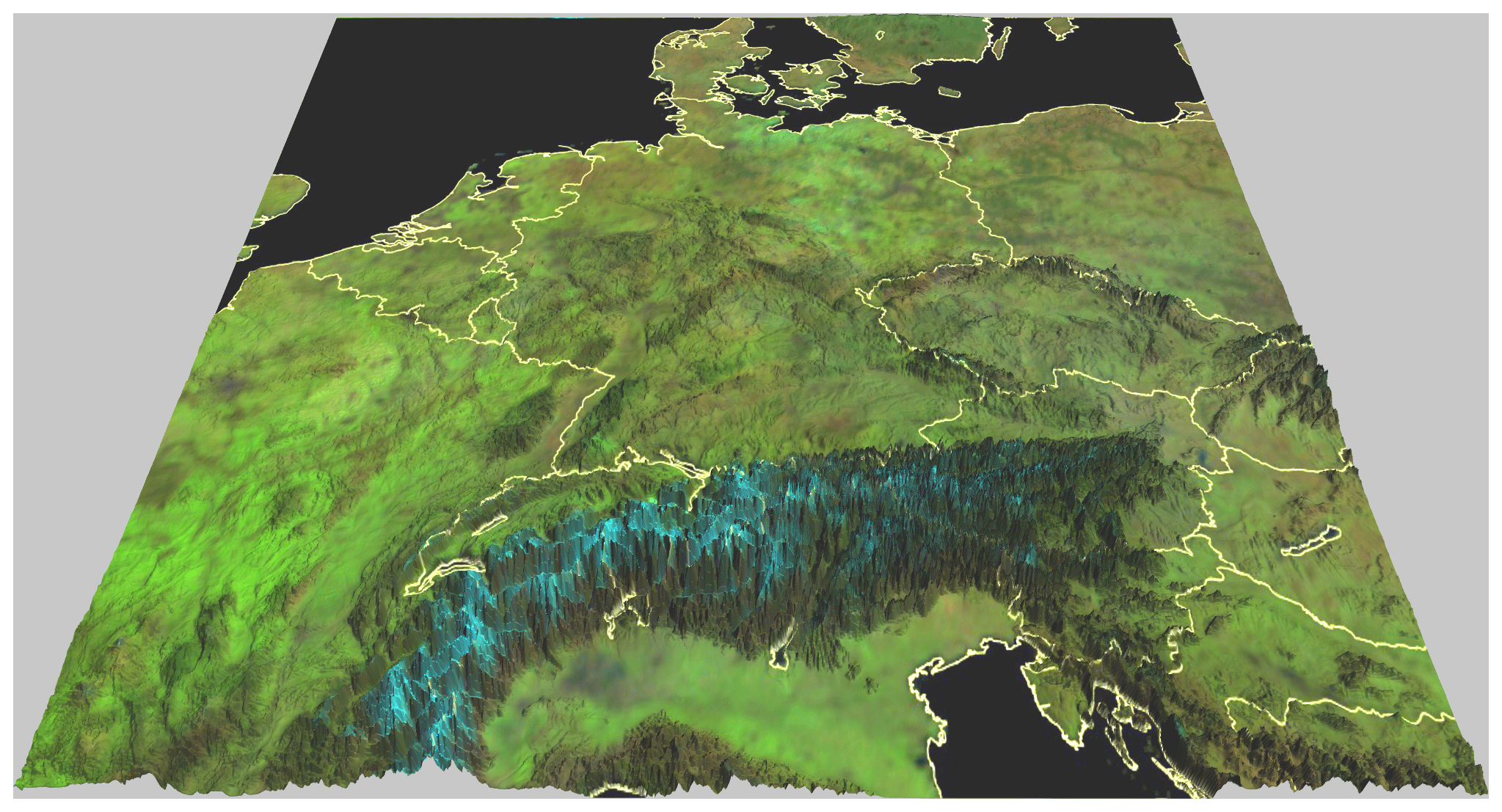
Figure 3Day-natural color RGB (red–green–blue) false-color composite based on the surface reflectance product of the LSA SAF at wavelengths of 1.6, 0.8, and 0.6 µm used by the improved retrieval scheme. The RGB texture has been overlaid on a three-dimensional perspective rendering of the elevation dataset used by the retrieval, which is derived from the SRTM15_PLUS digital elevation model. Country borders are shown as yellow lines.
In its current form, the retrieval scheme has been set up for a processing region of 240×400 standard-resolution pixels centered on Germany and central Europe. The domain can be seen in Fig. 3. To complement the improved spatial resolution with the highest possible temporal resolution, Meteosat's Rapid Scan Service is used as the primary input data stream. The relatively small processing region has been chosen to keep the processing time within reasonable bounds, as the pixel number increases by a factor of 9. Combined with the increased complexity in the algorithms introduced by the use of the HRV channel, the overall processing time is larger by about a factor of 15 compared to an identical low-resolution region.
More detailed descriptions of the individual steps of the processing and the used ancillary datasets are given in the following subsections.
3.1 NWC SAF cloud products
Within the improved scheme, several cloud products are generated from MSG SEVIRI observations based on the NWC SAF software in its 2016 version. From the NWC SAF cloud product suite, the cloud mask (CMa) and cloud type (CT) as well as the cloud-top pressure (CTP), height (CTH), and temperature (CTT) (Derrien and Le Gléau, 2005) are used. The cloud masking and typing schemes apply a set of multi-spectral threshold tests to derive an objective classification of the observed satellite scenery. Thresholds depend on solar illumination, viewing geometry, and a reasonable guess of the atmospheric state. For this purpose, the software provides climatological average values but can also employ forecast or reanalysis fields from numerical weather prediction models for improved accuracy. The cloud mask provides a binary distinction between cloud-free and cloud-contaminated or -filled pixels. Cloud typing divides cloud-containing satellite pixels into categories based on their height and opacity. Opaque clouds are classified into five classes: very low, low, medium, high, and very high clouds, which are separated by the pressure levels of 800, 650, 450, and 300 hPa. Additional classes distinguish between fractional clouds and high cirrus clouds with varying levels of opacity. The NWC SAF software currently does not separate between convective and stratiform cloud structures. The cloud-top height algorithm uses the radiative transfer code RTTOV (Saunders et al., 2018) as a forward model to relate the observed infrared radiances to those of a simulated cloud at a given vertical position and for given atmospheric conditions to infer the height of the top of clouds. For semitransparent clouds, either a CO2 slicing or a water vapor intercept method is applied (Borde et al., 2004).
3.2 Retrieval of cloud physical properties
Following the physical principles of bi-spectral retrievals described by Nakajima and King (1990), the CPP algorithm uses a measured reflectance pair at a visible (VIS) and a shortwave infrared (SWIR) wavelength, in this case from the SEVIRI 0.6 and 1.6 µm channels, to retrieve the cloud optical depth (τ) and effective particle radius (re).
Retrievals are performed assuming either a liquid or an ice cloud based on a determination of the cloud thermodynamic phase by a modified version of the Pavolonis et al. (2005) algorithm. Several spectral tests are performed based on observed SEVIRI brightness temperatures at 6.2, 8.7, 10.8, 12.0, and 13.4 µm, as well as clear- and cloudy-sky IR brightness temperature simulations with RTTOV. The algorithm initially yields five cloud types, which are further condensed into a classification of liquid and ice phase. More details are given in Benas et al. (2017).
CPP employs precalculated lookup tables (LUTs) of TOA cloud-top reflectances in a Rayleigh atmosphere, which have been simulated by the Doubling–Adding KNMI (DAK) radiative transfer model (Stammes, 2001). For water clouds, the droplet size distribution is assumed to follow a two-parameter gamma function with an effective variance of 0.15, while randomly oriented monodisperse imperfect hexagonal crystals are assumed for ice clouds. More details on the underlying single-scattering properties of the cloud particles can be found in Benas et al. (2017). The measured reflectances are corrected for absorption by atmospheric gases based on Moderate Resolution Atmospheric Transmission (MODTRAN4 version 3; Anderson et al., 2001) simulations. Subsequently, a match between the measurements and the LUT values of simulated reflectances is sought, which yields the cloud optical properties τ and re. Uncertainties of the retrieved values are estimated based on a 3 % relative error in the reflectances. A range of ancillary data is needed, including surface reflectance in the SEVIRI channels and vertically integrated column values of water vapor and ozone. The datasets used in the present scheme are listed in Sect. 3.4. Extensive details on the retrieval algorithm can be found in CMSAF (2016).
3.3 Solar irradiance
The SICCS algorithm (Deneke et al., 2008; Greuell et al., 2013) estimates solar irradiances at the TOA and surface from LUTs, which are calculated using the DAK model for cloud-free conditions, as well as for water and ice clouds. Both direct and global irradiances are calculated at the surface. A broadband version of DAK has been used for the calculation of the underlying LUTs, employing the correlated k-distribution technique to account for atmospheric gas absorption (Kuipers Munneke et al., 2008). For cloud-free pixels, aerosol properties (optical depth, Ångström parameter, and single-scattering albedo) are considered as input parameters, together with surface elevation, to estimate the resulting clear-sky irradiances. For cloudy pixels, the atmospheric transmission is further adjusted to account for the effects of cloud phase, τ, and re. For both cloudy and cloud-free pixels, the water vapor column, total ozone column, and surface albedo are taken into account and thus have to be provided as inputs.
Greuell et al. (2013) performed an extensive validation of the surface irradiance retrievals with European Baseline Surface Radiation Network (BSRN) measurements. Across all European sites, a median bias of 7 W m−2 (2 %) and a root mean square error (RMSE) of 65 W m−2 (18 %) were found for hourly values of surface irradiance.
3.4 Ancillary datasets
A number of ancillary input datasets have been modified in comparison to the original CPP/SICCS retrievals. The land–sea mask has been generated from the current version 2.3.7 of the Global Self-consistent Hierarchical High-resolution Shoreline (GSHHS) dataset (Wessel and Smith, 1996) for the considered region and the HRV grid. Surface elevation has been obtained from the SRTM15_PLUS digital elevation model (Tozer et al., 2019), which is based on the NASA Shuttle Radar Topography Mission (SRTM). It is available at a spatial resolution of 15 s (approximately 500 m), which is slightly higher than that of the HRV grid. Using this dataset, the much larger data volume of the original SRTM digital elevation models available at 30 and 90 m resolutions can be avoided.
Both the NWC SAF and CPP algorithms are configured to use numerical weather prediction input fields to account for the effects of the current atmospheric temperature and humidity profiles on infrared radiances by use of the RTTOV radiative transfer model. As input data streams, either the CAMS (Copernicus Atmospheric Monitoring Service) reanalysis (Inness et al., 2019) or the operational ECMWF forecast, together with aerosol properties from the CAMS forecast, can be used alternatively with 3-hourly resolution; the latter allows for near-real-time processing, while the former is only available with some time delay. In addition, the NWC SAF software uses the OSTIA dataset as input for sea surface temperature (Donlon et al., 2012). Spectral and broadband surface reflectance maps from the Land Surface Analysis Satellite Application Facility (LSA SAF; Carrer et al., 2018) are used in our modified version of the CPP algorithm to account for the effects of surface reflection on solar radiances. These have been re-projected to the HRV grid using bilinear interpolation. Within CPP and SICCS, the effects of atmospheric absorption by water vapor and ozone are accounted for using the vertically integrated column values obtained either from the CAMS reanalysis or from the ECMWF forecast. In addition, aerosol properties are represented in the SICCS scheme by using either the CAMS reanalysis or CAMS forecast as inputs. For this purpose, the aerosol optical depths at 468 and 865 nm are converted to a corresponding aerosol optical depth at 500 nm and the Ångström exponent, which are the input parameters expected by SICCS.
3.5 Use of the HRV channel
A high-resolution cloud masking scheme is an essential prerequisite for increasing the spatial resolution of SEVIRI cloud property retrievals, as uncertainties are expected to be largest for partly cloud-filled standard-resolution pixels. In particular, broken and inhomogeneous cloud fields are usually characterized by an abundance of such pixels (Werner et al., 2018). This implies that frequently only some of the nine sub-pixels in a cloudy standard-resolution pixel are actually cloudy, leading to false positive detections. Also, the higher resolution improves the detection of small-scale cumuli, which might go undetected at the coarser spatial resolution of the narrowband channels and result in false negative detections (Bley and Deneke, 2013).
The present study applies the threshold-based scheme introduced by Bley and Deneke (2013). Temporal averaging is used to obtain clear-sky reflectance composites for the HRV channel, while a regional threshold relative to the clear-sky composite is used to yield a binary classification of clear and cloudy observations. The Matthews correlation coefficient (MCC; Matthews, 1975) is used for threshold selection to quantify and maximize the accuracy of the resulting classification. Using a cloud mask obtained at standard resolution as a first guess, an iterative algorithm is applied to update the clear-sky reflectance composite and the threshold values, thereby optimizing the accuracy of the resulting HRV-based cloud mask. Details about the full algorithm, including the calculation of the HRV clear-sky composites and the selection of regional HRV reflectance thresholds, can be found in Bley and Deneke (2013). Compared to the original scheme, a number of updates have been made. First, the cloud mask and type from the NWC SAF v2016 software are now used as a basis instead of those provided by EUMETSAT's Meteorological Processing Facility. For derivation of the clear-sky composite and thresholds, observations are aggregated over 16 d and 1 h of observations (i.e., 12 RSS time slots) for a total of scenes. A temporal overlap of 8 d between successive analysis periods is used to ensure that the clear-sky composite can respond to rapid changes in surface reflectance. While the original scheme was based on regional thresholds, only three different thresholds for land, sea, and coastal areas are used in the present scheme to improve the overall stability. This classification is based on the land–sea mask obtained from the GSHHS dataset, as described in Sect. 3.4. Pixels containing both land and water in a neighborhood of 9×9 HRV pixels are considered to be coastal or shore. As the information content of the HRV channel for cloud masking is limited, a set of rules is used to combine the standard- and high-resolution cloud masks, considering blocks of 3×3 pixels, the HRV cloud mask, and the NWC SAF cloud type. Semitransparent high clouds are frequently missed by the HRV cloud mask and are thus labeled as cloudy based on the NWC SAF cloud type. The NWC SAF cloud mask does, however, frequently misclassify small clouds as cloud-free due to its coarser pixel resolution. Thus, pixels detected as cloudy by the HRV mask and as cloud-free by the NWC SAF mask are labeled as cloudy. The only exception to this rule are pixel blocks labeled as snow-covered land or sea ice by the NWC SAF cloud type algorithm, which are expected to be highly reflective and are thus left unchanged.
For the retrieval of cloud properties, a linear model is assumed following Cros et al. (2006) and Deneke and Roebeling (2010) to link the reflectances of the 0.6 µm, 0.8 µm, and HRV channels denoted by r06, r08, and rH, respectively:
For obtaining the coefficients a and b, an empirical least-squares regression is applied. Prior to the regression, the HRV channel images are first smoothed with the averaged MTF of the 0.6 and 0.8 µm channels, and they are subsequently downsampled to the standard resolution. Fit coefficients are again calculated for reflectances aggregated over 16 d and 1 h of observations. More discussion on the accuracy of this fit can be found in Cros et al. (2006) and Deneke and Roebeling (2010), as well as the analysis in Werner and Deneke (2020).
Within the modified CPP retrieval, Eq. (1) is not applied to the absolute values of reflectance, but only to their high-frequency residuals, which are defined as follows:
Here, denotes the actual reflectance field as observed with the HRV channel (i.e., sampled on the HRV grid and smoothed with the MTF of the HRV channel), while denotes the field sampled on the HRV grid but smoothed with the averaged MTFs of the 0.6 and 0.8 µm channels.
Solving for δr06, the following relation is found:
As this equation contains δr06 and δr08 as unknowns, a further constraint is required. While an empirical relation obtained from coarser spatial scales was used by Deneke and Roebeling (2010), the lookup tables of the CPP retrieval are utilized here. An initial value of δr06 is calculated from Eq. (1) by assuming that its value is equal to δr08. In each retrieval iteration, a refined value of δr08 is calculated by means of the following equation:
Here, ℱλ denotes a function which utilizes the CPP lookup tables as forward model of the channel reflectances, in this case at the wavelength λ=0.8 µm for a given set of cloud properties and ancillary input variables. Thus, this step does not depend on actual observations at 0.8 µm, but only relies on the lookup tables and ancillary data of the retrieval.
The simplest approach to implement the cloud retrievals is the assumption that δr16=0, i.e., that the high-frequency residual of the SWIR channel reflectance can be neglected. This assumption has, however, been observed to cause reduced accuracy of the effective radius in comparison to the standard-resolution retrievals (see Werner and Deneke, 2020, and the discussion in Sect. 4.1). Two other candidate approaches were considered in this study but were found to be suboptimal: the assumption of an adiabatic cloud and that the effective radius remains constant within a 3×3 pixel neighborhood.
Instead, the approach determined to be most accurate by Werner and Deneke (2020) is used here: it determines the high-frequency residual δr16=0 based on the tangent of the τ contour at the location of the standard-resolution reflectances in the Nakajima–King diagram (referred to as the lookup-table approach with slope adjustment in Werner and Deneke, 2020). Mathematically, this can be expressed as the slope of the τ contour at the point or, equivalently, as the ratio of the partial derivatives with respect to τ at that point:
This approach is illustrated in Fig. 4. For more details, readers are referred to the companion paper of Werner and Deneke (2020).
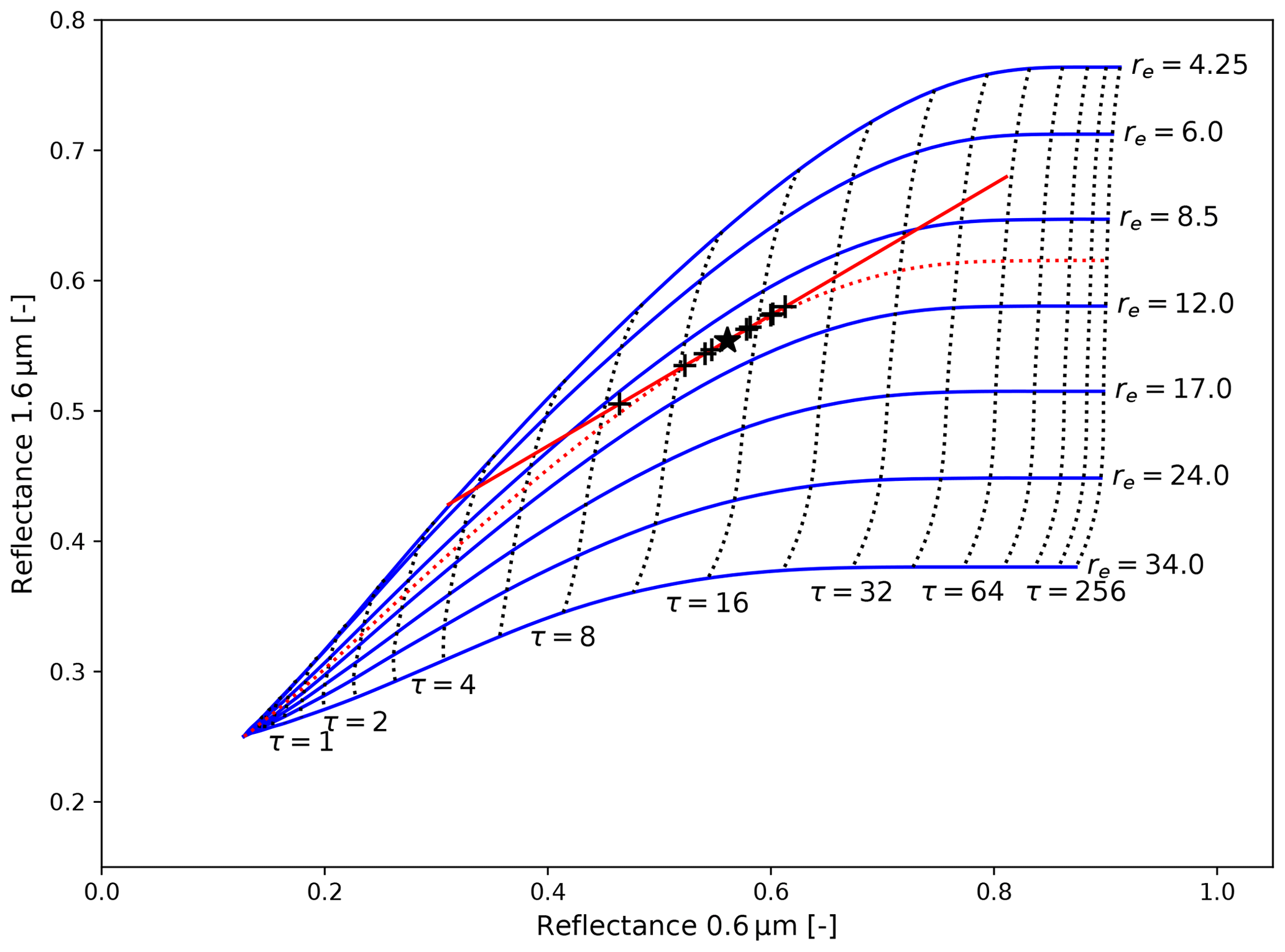
Figure 4Illustration of the lookup-table-based downscaling method with slope adjustment used in the improved HRV-based retrieval. The relation of the reflectances at wavelengths of 0.6 and 1.6 µm is shown for contours of pre-calculated cloud optical depth τ (dotted black lines) and effective radius re (solid blue lines) based on detailed radiative transfer calculations. A hypothetical standard-resolution observation with τ=14.0 and re=10.0 µm is marked by the black star. High-resolution retrieval results are marked by black crosses and are constrained to fall on the red line, which is given as tangent to the re contour at the point of the standard-resolution observation. See text for further explanation.
This section presents three application examples for the cloud products from the improved SEVIRI retrieval scheme. The examples have been selected to demonstrate the benefits that can be gained from the increase in spatial resolution and are compared to results obtained at SEVIRI's standard resolution.
4.1 Shallow convective clouds
The main motivation for the development of the HRV-based cloud retrieval scheme was the expectation that the increase in spatial resolution will lead to more accurate cloud retrievals and will bring the instrumental capabilities of SEVIRI closer to those of MODIS. Improvements are expected to be particularly significant for shallow convective clouds due to their comparatively small size and their large spatiotemporal variability.
To verify this aspect, a shallow convective cloud field is considered here, and retrieval results are contrasted with those obtained from collocated MODIS observations. A scene viewed by the MODIS instrument flown aboard the Terra Earth-observing satellite on 2 June 2013 at 10:50 Z over northeastern France has been selected for this purpose. The choice of observations from Terra allows the consistent use of MODIS retrievals based on the 1.6 µm channel for comparison with SEVIRI, as this channel of the MODIS instrument is affected by defective detectors on Aqua. While the satellite zenith angle of SEVIRI is about 55.6∘, the MODIS zenith angle is close to the nadir direction (2.7∘), which implies that the true pixel size is also close to the nominal spatial resolution of MODIS (1006×1007 m2). The scattering angles have values of about 155 and 150∘ for MODIS and SEVIRI, respectively.
The MOD06 cloud properties from the collection 6.1 release are used here for comparison (Platnick et al., 2017). It has to be pointed out that this comparison differs from that presented in Werner and Deneke (2020), where MODIS reflectances have been re-projected to the SEVIRI standard- and HRV-resolution grids first and then used as input to the CPP retrieval. In contrast, cloud products obtained from two independent retrievals and two different instruments are compared here. Hence, besides differences caused by the spatial resolution, the comparison is also affected by temporal changes due to the mismatch in observation times of about 1 min, the different observation geometries, and differences in the assumptions underlying both retrievals. Such assumptions include the width of the cloud droplet size distribution, which has values of 0.15 and 0.1 in the CPP and MODIS retrievals, respectively (Benas et al., 2019). A scene with scattering angles outside the cloud bow and cloud glory has been selected to minimize this sensitivity. The reflectances observed by SEVIRI will also include a significant contribution from cloud sides due to the large satellite viewing angle, while the nadir view of MODIS implies that reflected radiation mainly originates from the cloud tops. Retrieval results will also depend on the assumed values of surface reflectance. Thus, deviations are expected to be substantially larger than the differences reported in Werner and Deneke (2020).
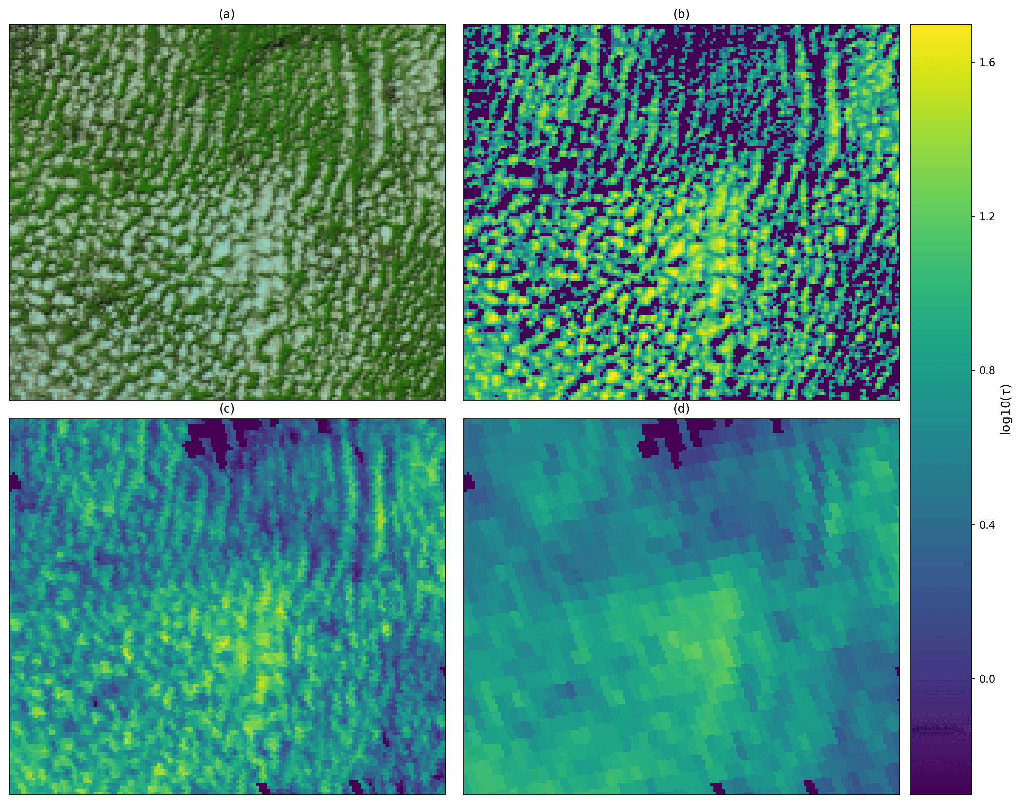
Figure 5Shallow convective cloud field observed over northeastern France at 3∘25′ E and 48∘7′ N on 2 June 2013 at 10:50 Z. MODIS reflectances are displayed as a day-natural color RGB composite in (a), and retrieved values of cloud optical depth (τ) are shown for the operational Terra MODIS C6.1 retrieval (b), the improved Meteosat SEVIRI retrieval (c), and the standard-resolution Meteosat SEVIRI retrieval (d) using a logarithmic color scale.
Figure 5 shows the fields of τ obtained for the example scene provided by MODIS and both the standard and improved HRV-based SEVIRI retrievals together with the day-natural color RGB rendering of the MODIS reflectances (Lensky and Rosenfeld, 2008). SEVIRI data have been re-projected to the MODIS grid using nearest-neighbor interpolation, and a translation has been applied to account for parallax shift and cloud motion in combination with the mismatch in observation time. This translation has been determined by maximizing the cross-correlation of both τ fields and results in a shift of the SEVIRI data by about 2.6 and 0.4 km in the north and east directions, respectively. While 83.8 % of the pixels are classified as probably or likely cloudy by the MODIS cloud mask, τ retrievals are reported for 72.4 % of the pixels (43.6 % and 28.8 % in the Cloud_Optical_Thickness_16 and Cloud_Optical_Thickness_16_PCL datasets, respectively), with a remaining 11.3 % of pixels without valid retrievals. In the case of the SEVIRI-based CPP retrievals, the quality flags showed that for 44.8 % and 33.3 % of the pixels for standard- and high-resolution retrievals, convergence could only be achieved for the 0.6 µm reflectance, and the observed 1.6 µm reflectance exceeded the range of values of the LUT, indicating in particular that the use of the HRV channel improves the fraction of pixels with high-quality retrievals.
It is clearly visible that the increased spatial resolution obtained by using the HRV channel in the retrieval helps to better resolve the small-scale structure of this cloud field. This visual impression is quantitatively confirmed by a significantly higher correlation coefficient of about 0.78 found for the HRV-based τ field and the corresponding MODIS C6.1 product compared to a value of 0.47 obtained for the standard-resolution retrieval results. Both fully overcast and partially cloudy retrieval results have been included in the calculation. Figure 6 shows the corresponding histograms of the derived τ using logarithmic bin spacing for this scene. The standard-resolution SEVIRI retrieval exhibits the narrowest distribution of values, with too few optically thin and thick clouds compared to the MODIS product. While the HRV-based SEVIRI retrieval still yields fewer optically thick clouds than MODIS, it reports a similar amount of optically thin cloud and is able to better reproduce the dynamic range of the MODIS product than the standard-resolution retrieval scheme. For the standard retrieval, the maximum value of retrieved τ is only 16.5, while values of 40.3 and 61.8 are observed for the SEVIRI HRV-based and MODIS products, respectively. A likely explanation for the remaining underestimation of cloud optical depth is the oblique viewing angle of Meteosat over Europe, which increases the pixel size in the north–south direction by a factor of about 2. Combined with the optical resolution of SEVIRI, which is lower than the sample resolution by a factor of 1.6, this results in a 5-fold larger pixel area despite a nominally equal nadir sampling resolution. While it is beyond the scope of the present article to fully resolve and explain the remaining discrepancies, they are likely due to the combined effects of differences in retrieval algorithms, sensor calibration, pixel resolution, and/or viewing geometry.

Figure 6Histograms of cloud optical depth (τ) using logarithmic bin spacing for the cloud field displayed in Fig. 5. Values are shown for the standard-resolution SEVIRI retrieval (a, blue), the improved HRV-resolution Meteosat SEVIRI retrieval (b, red), and the Terra MODIS C6.1 retrievals (c, red). The contribution of partially cloudy pixels to the MODIS histogram is indicated by a dotted line. Also, for each histogram, the values of the 25th, 50th, and 75th percentile are shown as a dotted line listed numerically.
It should be noted that for solar energy applications, the correct representation of τ values at and below a value of 5 is highly relevant, as such values will result in nonzero direct irradiance. While rejecting such retrieval results in the cloud retrieval scheme due to their large uncertainties will most likely improve the τ-retrieval accuracy itself, it will cause a subsequent overestimate of SSI if these pixels are assumed to be cloud-free. Both global and direct irradiance components will be affected, but errors will be most pronounced for the direct irradiance and the direct–diffuse ratio, which are parameters critical for the calculation of the tilted irradiance, e.g., on the plane of a photovoltaic module or the focal plane of a concentrating solar power plant.
Broken and inhomogeneous cloud fields such as the considered scene are known to be particularly problematic for the accuracy of the retrieved effective radius (Marshak et al., 2006; Wolters et al., 2010), and the following results should be interpreted with caution. For a meaningful comparison, only pixels with τ>8 in all compared datasets and high-quality retrieval results have been considered (full convergence of CPP retrievals, no partially cloudy retrievals from MODIS). These criteria are fulfilled for only 21.5 % of the pixels. Mean values of 8.2, 7.7, and 7.3 µm are found for MODIS and the standard- and high-resolution effective radii retrievals, respectively. The correlations between MODIS- and SEVIRI-based effective radii are much lower than those for optical depth, and only a slight improvement is found from the use of the HRV channel for the retrieval, with Pearson correlation coefficients of 0.43 and 0.39 for the HRV and standard-resolution effective radius results, respectively. The reader is reminded that a similar magnitude of the correlation is expected, as the retrieval constraint for the 1.6 µm channel ensures that the effective radius is close to that of the standard-resolution retrieval. This is confirmed by a comparatively high correlation coefficient of 0.88 between the SEVIRI results at the different spatial resolutions. A modification of the retrieval to only use a smoothly interpolated value of the 1.6 µm reflectance instead results in a slightly negative value of −0.04 for the correlation of the high-resolution effective radius retrieval with MODIS re. This finding emphasizes the fact that despite the seemingly low values of correlation for re reported above, the choice of the retrieval constraint is important to ensure that the accuracy of the standard-resolution re is not degraded by use of the HRV channel.
4.2 Detection of convection initiation
An application which is expected to benefit from the improved high-resolution SEVIRI cloud property retrievals is the early detection of convective initiation (CI). Current approaches for the SEVIRI instrument are mainly based on the narrowband channels and are thus limited to the standard spatial resolution of SEVIRI (e.g., Mecikalski et al., 2010). Some previous studies have already pointed out benefits arising from the use of the HRV channel (e.g., Carbajal Henken et al., 2011; Mecikalski et al., 2013a; Merk and Zinner, 2013). While the first satellite-based CI detection schemes were based on observed radiance fields (Mecikalski and Bedka, 2006), the use of cloud properties instead of radiances seem promising, as it should remove covariability with environmental influences and viewing geometry, and it should aid a more physical interpretation of cloud growth (e.g., Senf and Deneke, 2017). It has thus been considered in several more recent scientific studies (e.g., Mecikalski et al., 2011, 2013b). The combination of cloud products and higher spatial resolution offered by the HRV channel could thus be one way to improve the lead time for the detection of convective initiation in current MSG-based CI detection schemes. In particular, developing convective clouds can likely be resolved earlier in their life cycle, and small-scale variability of convective clouds can be better resolved.
To illustrate this aspect, an example case considering the early growth phase of a deep convective cloud system which formed on 18 June 2013 is presented here. On this day, a series of orographically triggered thunderstorms developed along the mountain range of the Thuringian forest. The weather over central Europe was dominated by an upper-level high-pressure ridge, with an extension from northern Africa to southwestern and central Europe. An upper-level low-pressure system was located over the Iberian Peninsula, and advected hot and unstable air masses northward towards central Europe on the forward flank of its frontal zone. This led to an unstable atmospheric situation with extremely high values of mixed-layer convective available potential energy (CAPE) reaching up to 3600 J kg−1 over southern and central Germany, as diagnosed from the Global Forecast System reanalysis2. The first shallow convective clouds started to form around 10:30 Z along the Thuringian forest.
The convective cell considered here initiated at a location and time of 11∘16′57′′ E, 50∘29′30′′ N and 13:50 Z, developed into a cold-ring storm (Setvák et al., 2010), and lasted for more than 5 h before dissipating around 19:30 Z. An increase in radar reflectivity above a threshold of 35 dBZ has been adopted to determine the location and timing of CI for this cell (Senf and Deneke, 2017), based on observations from the German weather radar network.
Figure 7 shows a time sequence of frames of the day-natural color RGB composite based on SEVIRI's 1.6, 0.8, and 0.6 µm reflectances downscaled to HRV resolution, overlaid with contours of the 10.8 µm brightness temperature for a time period from 13:30 to 14:10 Z and centered on the location of CI. At 13:30 Z, thus 20 min prior to CI, the cell started to grow rapidly in vertical extent. Beginning as a rather small and shallow cloud with a minimum cloud-top temperature around the freezing level, it reached 260 K 5 min later and values below 240 K at 13:45 Z.
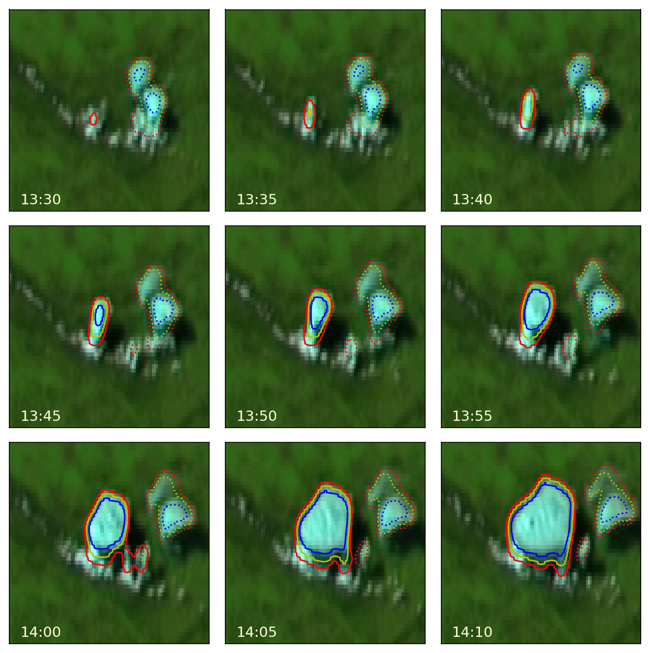
Figure 7Time sequence of the day-natural color RGB composite showing the SEVIRI reflectances for the 1.6, 0.8, and 0.6 µm channels, downscaled to HRV channel resolution using the constant-reflectance ratio approach described in Werner and Deneke (2020). Frames correspond to a time period from 13:30–14:10 Z on 18 June 2013 and a region of 51×101 pixels (about 100×100 km2) centered on the location of convective initiation occurring at 11∘16′57′′ E and 50∘29′30′′ N. An aspect ratio of 2 : 1 is used to compensate for the lower pixel resolution in the north–south direction. Also shown are contours of the 10.8 µm brightness temperature (red: 273.15 K; yellow: 260 K; blue: 240 K). Solid lines are used for the convective cell of interest, while dotted lines are used for other cells.
In the following analysis, pixels belonging to the convective cloud object of interest have been identified using an adaptive threshold in 10.8 µm brightness temperature. For this purpose, an object mask has been constructed using a threshold which is 5–20 K warmer than the observed minimum brightness temperature, increasing the spread linearly from 5 K at 273.15 K to 20 K at 220 K and keeping it constant above or below this range. Figure 8 shows a comparison of the temporal evolution of τ for the convective cell based on results from the improved high-resolution and standard-resolution retrievals. For this purpose, the standard-resolution τ retrieval has been interpolated to the HRV grid using bilinear interpolation for consistency. In the early stages of the cloud life cycle starting at 13:20 Z, some pixels already show optically thick τ values exceeding 50 for the high-resolution retrieval. In contrast, maximum values of τ remain below 20 up to 13:40 Z for the standard-resolution retrieval. A notable increase in the median of τ can be seen at 13:30 and 13:40 Z for high- and standard-resolution τ results, respectively. This implies that, at least for the considered convective cell, growth signatures in τ are found about 10–20 min earlier for the high-resolution retrievals depending on the considered quantity, potentially increasing the lead time for the detection of CI.
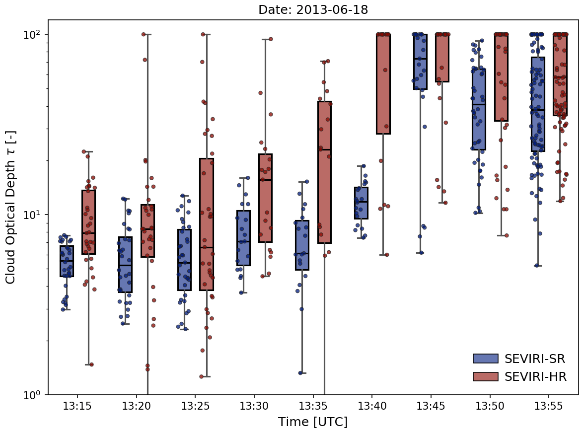
Figure 8Box-and-whisker plot of cloud optical depth (τ) as a function of time for the convective cell shown in Fig. 7, comparing the standard-resolution retrieval (SEVIRI-SR, blue) and the improved HRV-based retrieval (SEVIRI-HR, red). A time period from 13:15–13:55 Z has been chosen to capture the early growth phase of the convective cell. The boxes extend from the lower to the upper quartile, the lines within the boxes mark the median, and the whiskers extend to the minimum and maximum values of τ for all pixels belonging to the cloud object. Additionally, points have been added displaying the individual τ values of the object pixels.
4.3 Surface solar irradiance
In this subsection, benefits of the increased spatial resolution of the improved retrieval scheme for estimating SSI are discussed. In climate studies, it is usually sufficient to average radiative fluxes over longer time periods (e.g., Wild, 2020). In contrast, various authors (e.g., Wiemken et al., 2001; Perpiñán et al., 2013; Lave et al., 2015) have demonstrated the need to quantify irradiance variability in the 1 min or even 1 s range in order to capture the full range of natural fluctuations relevant for the grid integration of solar power generation.
High-frequency variability is introduced by clouds with sizes smaller than the pixel resolution, small-scale cloud heterogeneity, and three-dimensional (3D) radiative transfer effects and can even result in enhanced irradiances (Schade et al., 2007). Such effects are poorly represented in satellite-based SSI products due to their reliance on 1D radiative transfer (Deneke et al., 2005) and due to under-sampling in space and time by satellite observations. In particular, the high correlation of TOA and surface fluxes implied by 1D radiative transfer breaks down for 3D radiative transfer (Kassianov et al., 2005), resulting in a decorrelation of atmospheric transmission and reflection as seen in ground-based and satellite observations (Deneke et al., 2009). It is of high scientific relevance which part of the SSI variability is missed by satellite retrievals and how this is affected by the spatial and temporal resolution of satellite observations. In the following case study, it is thus investigated how the increase in spatial resolution of the improved HRV-based retrieval changes the agreement of satellite-based SSI with surface observations.
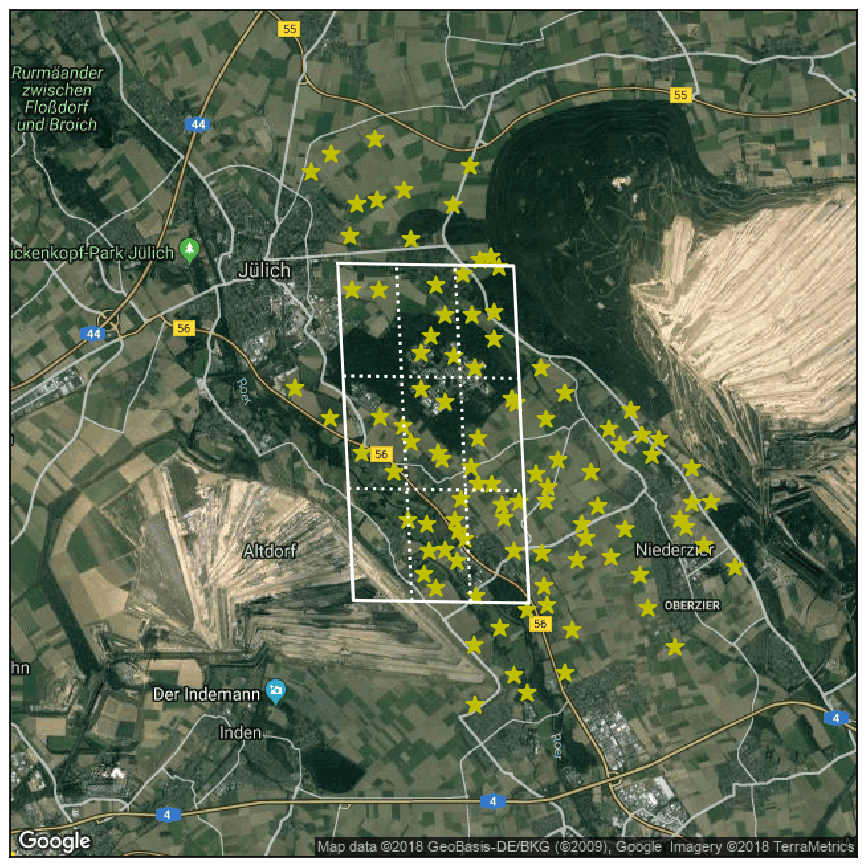
Figure 9Google Maps™ satellite view showing the measurement region of the pyranometer network operated during the HOPE campaign in the vicinity of Jülich, Germany, in spring and summer of 2013. The individual pyranometer stations are marked by yellow stars, the location of the corresponding standard-resolution MSG SEVIRI pixel is shown by solid white lines, and the 3×3 HRV pixels laying within this pixel are delimited by the dotted lines. Map data: © Google, GeoBasis, and TerraMetrics.
As a reference, a unique dataset of observations from a dense pyranometer network operated during the High Definition Clouds and Precipitation for advancing Climate Prediction (HD(CP)2) Observational Prototype Experiment (HOPE) is used here. HOPE was a field experiment that took place in Jülich, Germany, from 3 April to 31 July 2013 (Macke et al., 2017). It was conducted to provide a broad range of observational datasets for the evaluation of the atmospheric icosahedral non-hydrostatic (ICON) model developed within the HD(CP)2 project (Heinze et al., 2017). Each of these stations was equipped with a silicon photodiode pyranometer (model: EKO ML-020VM) to measure the global horizontal irradiance at 10 Hz resolution, a micromodule to measure air temperature and relative humidity (Driesen+Kern DKRF 4001P), and an embedded Global Positioning System (GPS) module as an accurate time reference. A description of the network and the resulting dataset is given in Madhavan et al. (2016). An overview of the distribution of stations is shown in Fig. 9. As the stations were placed within an area of only 8×10 km2, many of the inter-station distances were smaller than the SEVIRI pixel resolution, even for its HRV channel. This unique dataset can thus provide novel insights into the small-scale variability of global irradiance unresolved by current geostationary satellite observations. Madhavan et al. (2017) introduced methods to estimate the deviation between a point measurement and the spatial average for a surrounding domain, as well as how spatial averaging affects the power spectrum of the corresponding SSI time series. Due to the large number of pyranometers, robust evaluation statistics can be obtained even for single days; 24 May 2013 has been chosen here as a case study. The weather on this day was influenced by an upper-level trough in combination with a northwesterly airflow, advecting polar air masses to central Europe and leading to convective activity and showers. The occurrence of cumulus congestus together with relatively strong winds caused significant variability in the SSI.
For each station, a matching satellite-based time series has been extracted from the standard- and HRV-resolution satellite products, weighting pixels by a Gaussian centered on the station location with a standard deviation of 1 km in the north–south and east–west directions, respectively, and accounting for the distorted shape of satellite pixels due to the oblique viewing geometry. A shift in collocation has been applied here to maximize the daily correlation between ground-based and satellite time series, having a magnitude of 2700 and 3000 m in the west and north directions, respectively. A time period from 08:00 Z in the morning until 16:00 Z in the afternoon has been considered, and the time series of the 63 stations that passed the quality control criteria described by Madhavan et al. (2016) are included in the analysis. The SSI time series have been smoothed using a 5 min running mean before subsampling to the observation time of SEVIRI, accounting for the delay between the start of the scan and acquisition time for the considered region.
Figure 10 shows the median time series together with the interquartile range (25th–75th percentile) and the 5th–95th percentile range obtained from the pyranometer observations and the two satellite-based retrievals. The statistics for both satellite datasets and the pyranometer observations are calculated consistently based on the time series obtained at the location of the pyranometer stations. High spatiotemporal variability is observed, as indicated by the large range of values at specific times and large temporal changes throughout the day. The pyranometer-based dataset (black) clearly exhibits the largest spatiotemporal variability, while the HRV-based product (red) also shows notably more variability than the standard-resolution product (blue). It also seems to capture the variability of the pyranometer dataset better. Specifically, minima and maxima in the pyranometer record appear to be better resolved. In particular, the standard-resolution SSI data show an overestimate for thicker clouds, consistent with the underestimation of τ values for optically thicker clouds already discussed in Sect. 4.1 and Fig. 6.
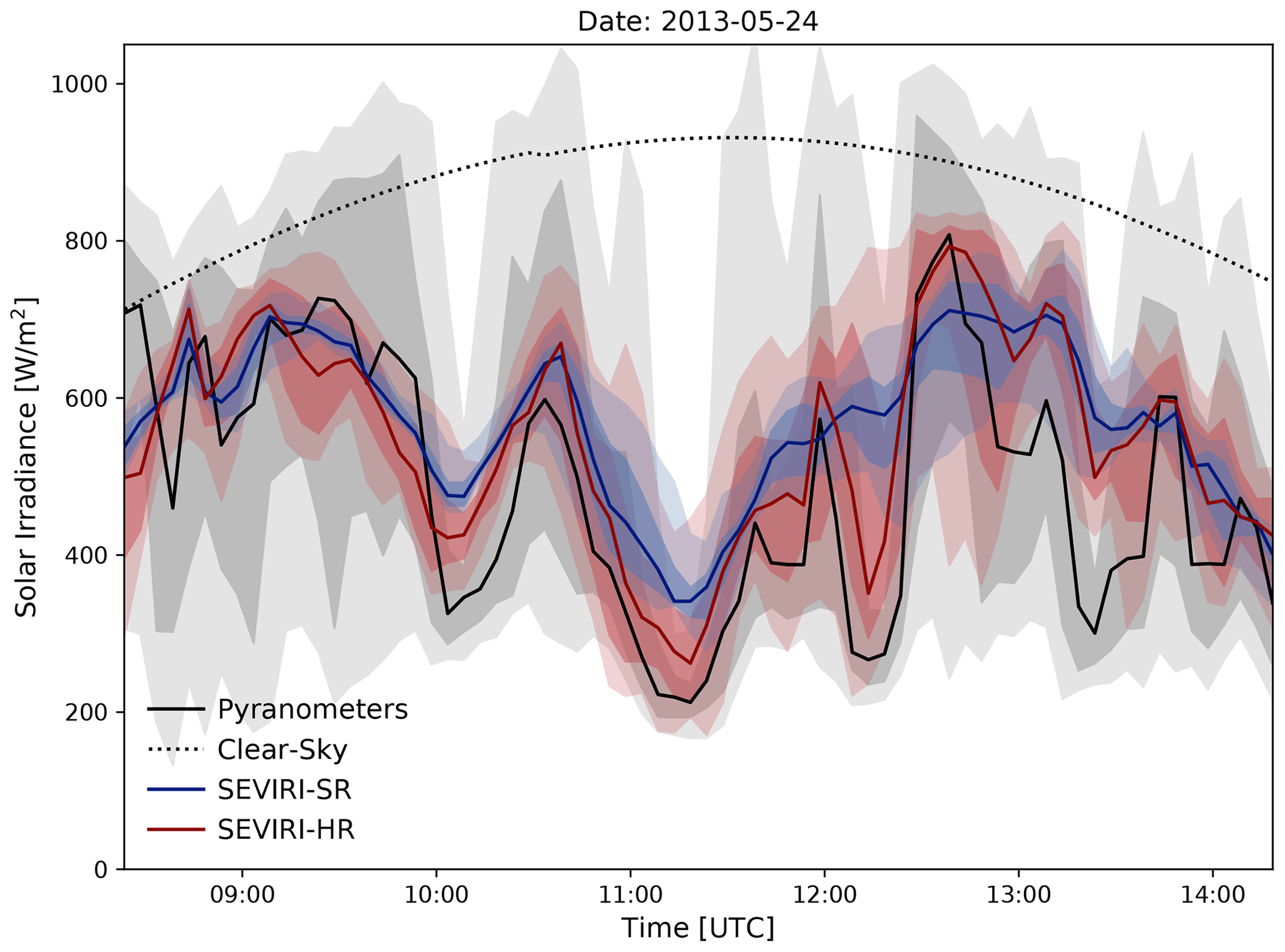
Figure 10Time series of ground-based and SEVIRI-retrieved surface solar irradiance. The median (thick line), interquartile range (dark shading), and 5th–95th percentile range (light shading) of SSI reported by the 63 pyranometers at the stations in Fig. 9 (black) are shown, visualizing the spatial variability across the stations. The corresponding time series obtained from the standard-resolution (SEVIRI-SR) and the improved HRV-resolution (SEVIRI-HR) SEVIRI retrievals at the station locations are displayed in identical style using blue and red, respectively. All time series have been resampled to the 5 min time resolution of the SEVIRI observations. The mean clear-sky irradiance from the satellite retrieval is shown as a dotted black line.
To support this visual impression, Fig. 11 displays the root mean square error (RMSE) for the two satellite-based products using the pyranometer irradiance as a reference. The RMSE is derived for several averaging periods between 5 min and 1 h. A strong reduction of RMSE with averaging period is observed: while for 5 min averages, RMSE values of 184 and 200 W m−2 are found, this is reduced to 58 and 64 W m−2, respectively, for hourly averages. Regardless of averaging period, a reduction of the median RMSE by about 10 % is found for the HRV-based product. Applying Mood's median test (Mood, 1950) to test the difference of the distributions, a reduction is found for the RMSE, which is statistically significant at the 95 % confidence level for all but the 30 min averaging period.
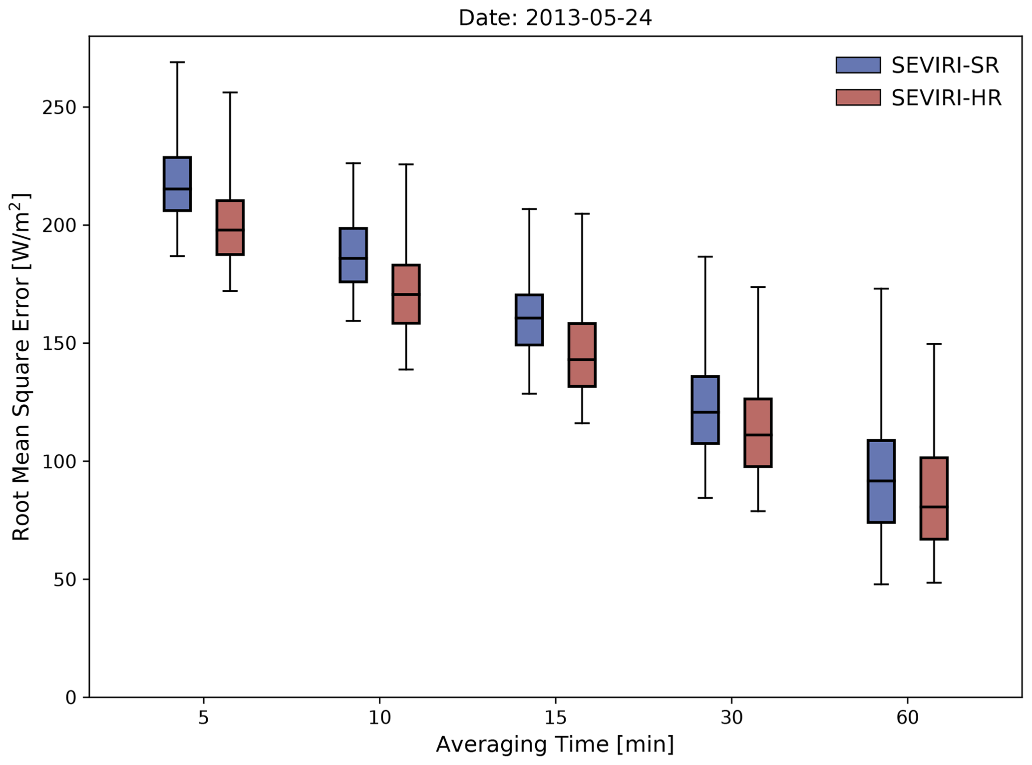
Figure 11Distribution of the daily-mean root mean square error (RMSE) found from the comparison of pyranometer-based and satellite-derived SSI time series for the 63 pyranometer stations for 24 May 2013. A box-and-whisker plot is used for visualization, and averaging periods ranging from 5 min to 1 h are considered. Boxes extend from the lower to the upper quartile, the line within the boxes displays the median, and the whiskers extend to the minimum and maximum values. Results are shown for standard-resolution (SEVIRI-SR) and high-resolution (SEVIRI-HR) SSI retrievals in blue and red, respectively.
It is worth pointing out that the interquartile ranges of the RMSE for different stations and averaging periods have a magnitude of about 20–30 W m−2 and that the distributions partly overlap for the two satellite-based SSI products. Hence, without the large number of stations in the pyranometer network, it would not have been possible to diagnose the accuracy improvement achieved by the HRV-based SICCS product for this case study with any statistical confidence. While additional days or observations across a larger region could have been used, this complicates a comparison by combining observations with different cloud types and synoptic conditions, which are both factors that are likely to influence the absolute product accuracy and the sensitivity to spatial resolution. A further interesting aspect is the sensitivity of the RMSE to the applied shift in collocation, which is particularly strong for the HRV-based retrieval. While we have empirically chosen an optimal collocation here, this raises the question of how to collocate ground-based and satellite observations in an operational setting, which is an aspect that becomes more important with increased spatial resolution.
Within the present paper, it has been demonstrated that it is possible to improve the spatial resolution of MSG SEVIRI-based cloud property and subsequent SSI retrievals by use of its HRV channel. For this purpose, the HRV reflectance is first used in a threshold-based cloud mask, while the high-frequency component of the HRV reflectance is subsequently extracted with a high-pass filter and utilized as a physical constraint to resolve small-scale variability in cloud optical depth. As no information is available on the small-scale variability of effective radius, a constraint based on the lookup tables used by the cloud property retrieval has been implemented in the present version of the algorithm.
An overview of the complete retrieval scheme has been given here, including a description of the modifications made to the CPP retrieval to utilize the HRV reflectances for improving the spatial resolution, the ancillary data incorporated into the scheme to optimally benefit from the improved spatial resolution, and some other changes to improve the base retrieval. A more in-depth evaluation of the applied downscaling algorithm, an evaluation of its accuracy based on MODIS observations, and a discussion of the choice of the constraint imposed for the effective radius can be found in the companion paper by Werner and Deneke (2020).
Three applications of the resulting cloud and radiation products have been presented to highlight some benefits arising from the improved spatial resolution. First, operational MODIS C6.1 and SEVIRI retrievals of τ and re have been compared for a shallow convective cloud field, showing better agreement and enhanced capabilities to resolve the small-scale variability of τ. The initiation and growth phase of a severe convective storm has been analyzed, indicating that the formation of an optically thick cloud corresponding to the growing convective cell can be recognized 10–20 min earlier. This case study shows promise for improving the detection of convection initialization in the future. Finally, the retrieved time series of SSI has been compared with observations from a dense pyranometer network, showing a statistically robust improvement in the agreement of the satellite retrievals with the ground-based observations, leading to a reduction of the RMSE by about 10 %.
Future work in several directions is warranted. While the present version of the retrieval algorithm already seems to yield results superior to those of the standard-resolution scheme, we do believe that there are several aspects of the algorithm that can be further improved. This includes the treatment of small-scale variability in effective radius, either by using physical constraints such as the adiabatic model (see, e.g., Merk et al., 2016) or empirical parameterizations, possibly adapted to the local cloud type. The use of corrections for partially cloud-filled pixels, such as those proposed by Werner et al. (2018), is also expected to be beneficial. Complementary ideas for using the HRV channel to correct infrared brightness temperatures for effects of partially cloudy pixels and to improve estimates of cloud-top temperature have been presented by Mecikalski et al. (2013a).
The method described here and in Werner and Deneke (2020) can also be adapted to other meteorological multi-resolution imagers such as the Advanced Baseline Imager aboard the current generation of geostationary GOES satellites, the Flexible Combined Imager on the upcoming Meteosat Third Generation, and the polar-orbiting MODIS instruments. This would allow for increasing the spatial resolution of the retrieved cloud and radiation products to 500 m for GOES-R and MTG and to 250 m for MODIS. These instruments have in common that they feature a higher-spatial-resolution visible channel, which allows constraining cloud optical depth (e.g., the 0.6 µm channel with 250 and 500 m resolution for MODIS and GOES-R ABI, respectively), and lower-resolution SWIR channels (e.g., 1.6 or 2.2 µm) used as a constraint for the cloud effective radius in bi-spectral retrievals. In fact, the constraint imposed due to the relatively broad spectral width of the HRV channel formalized by Eq. (3) would no longer be required. Only the constraint on the small-scale variability in SWIR reflectance expressed by Eq. (5) would be needed, thus allowing a simplified implementation. It should be noted, however, that based on the findings presented here and in Werner and Deneke (2020), an overly simplistic constraint as, e.g., realized by simple interpolation of the absorbing-channel reflectance will lead to reduced accuracy for cloud effective radius, which might in fact be worse than that of a retrieval done at the lowest common spatial resolution. It also has to be stressed that a higher spatial resolution does not necessarily imply higher product accuracy. Specifically, the findings of Zinner and Mayer (2006) suggest that at resolutions higher than 1 km, three-dimensional effects become more prominent, causing increasing deviations from the assumption of 1D radiative transfer underlying current retrievals. In addition, the use of cloud-absorbing reflectances at other wavelengths in the cloud property retrieval, e.g., at 2.2 µm, might influence the accuracy of the downscaling algorithm.
Despite these caveats, the comparison or even synergistic combination of satellite and ground-based observations critically depends on the collocation of the observations in terms of the sampled atmospheric volume. At least in this respect, an improved spatial resolution of the satellite products is likely always beneficial due to the fact that most ground-based observations are able to resolve much finer-scale cloud structures.
In future work, a more extensive evaluation of the resulting product quality should be conducted. Specifically, the results presented here for the three example applications should be extended to a larger number of satellite scenes in order to confirm the representativeness of the findings. A number of additional products are derived from satellite observations based on τ and re. Examples are the cloud liquid water path and droplet number concentration, as already considered in Werner and Deneke (2020), and the SEVIRI-based estimation of rain rate (see, e.g., Roebeling and Holleman, 2009).
Concrete plans exist in particular to further investigate the dependence of the accuracy of SSI retrievals on the spatial and temporal resolution of the satellite data due to the relevance of satellite-based SSI products for solar energy applications. Specifically, a comprehensive evaluation against data from the pyranometer network is planned, including the MetPVNet measurement campaigns in autumn 2018 and summer 2019, which cover a different region and different cloud conditions. Meilinger et al. (2020) find deviations of up to ±600 W m−2 depending on cloud type when comparing CAMS satellite products and ground measurements of solar irradiance with a temporal resolution of 1 min for the first of these campaigns.
Finally, while some of the benefits of the presented scheme will be available in the future by use of observations from the Meteosat Third Generation (MTG) Flexible Combined Imager, climate applications often depend on the availability of long-term records. Hence, even after launch of MTG, the SEVIRI-based scheme might present a pathway toward creating a more homogeneous long-term climate data record of cloud properties at 1 km spatial resolution based on both MTG and MSG observations.
The datasets used for the analyses presented in this paper and the Python codes used for preparing the CPP input and paper figures are publicly available from the Zenodo data repository via https://doi.org/10.5281/zenodo.4936573 (Deneke et al., 2021). Meteosat SEVIRI level 1.5 data can be obtained from the EUMETSAT Data Centre at https://eoportal.eumetsat.int/userMgmt/protected/dataCentre.faces (last access: 19 May 2021, Schmetz et al., 2002). The MODIS data used here can be obtained from the Level-1 and Atmosphere Archive and Distribution System Distributed Active Archive Center via https://ladsweb.modaps.eosdis.nasa.gov/ (last access: 19 May 2021, Platnick et al., 2017). The CPP retrieval software is copyrighted by EUMETSAT and is not publicly available. The NWC SAF software can be obtained by registered users from http://www.nwcsaf.org/ (last access: 19 May 2021, Fernandez et al., 1999). LSA SAF products can be obtained by registered users from https://landsaf.ipma.pt/ (last access: 19 May 2021, Carrer et al., 2018). The CAMS reanalysis is available from the Atmosphere Data Store at https://atmosphere.copernicus.eu/data (last access: 19 May 2021, Inness et al., 2019). The SRTM_15PLUS dataset can be obtained from https://topex.ucsd.edu/pub/srtm15_plus/ (Tozer et al., 2019). The GSHHG dataset can be obtained from https://www.soest.hawaii.edu/pwessel/gshhg/ (Wessel and Smith, 1996).
HD was responsible for conceptualization. HD, SB, FW, and MSH prepared the methodology. HD, SB, PW, JFM, FS, and FW developed software. HD, CBV (Sect. 4.3), SL (Sect. 4.2), MSH, FS (Sect. 4.2), JW (Sect. 4.3), and FW conducted the formal analysis. HD, CBV (Sect. 4.3), SL (Sect. 4.2), JFM (Sect. 3.2), MSH, FS (Sects. 3.1 and 4.2), JW (Sec 4.3), and FW prepared the original draft. HD, AH, AM, and MSH acquired funding. All authors contributed to review and editing, and all authors have read and agreed to the accepted version of the paper.
The authors declare that they have no conflict of interest.
Publisher's note: Copernicus Publications remains neutral with regard to jurisdictional claims in published maps and institutional affiliations.
The authors thank Stefanie Meilinger for initiating the MetPVNet project and for her valuable comments on an earlier version of this paper. Also, the comments by two anonymous referees on the discussion paper helped to significantly improve the final paper and are gratefully acknowledged. The initial concept for this investigation was conceived during a EUMETSAT research fellowship of the first author hosted at KNMI. The associated financial support and discussions with scientists at EUMETSAT and KNMI are greatly appreciated. This study was carried out within the framework of the German collaborative project MetPVNet funded by the German Ministry of Commerce under grant number 0350009E. The use of the following data and software is gratefully acknowledged: SEVIRI satellite data distributed by EUMETSAT and obtained from the TROPOS satellite archive; MODIS data obtained from the Level-1 and Atmosphere Archive and Distribution System (LAADS) Distributed Active Archive Center (DAAC); surface albedo data generated and distributed by the LSA SAF; CAMS reanalysis data obtained from the Copernicus Atmosphere Monitoring Service; the GSHHG dataset developed and maintained by Paul Wessel (SOEST, University of Hawaii, Honolulu, HI) and Walter H. F. Smith (NOAA Geosciences Lab, National Ocean Service, Silver Spring, MD); the SRTM15_PLUS topography provided by the Satellite Geodesy research group at the Scripps Institution of Oceanography; the NWC/GEO software package developed and distributed by the NWC SAF; the CPP software developed by KNMI as part of the CM SAF; and various open-source software packages used for this work, including the Python programming language and various SciPy packages. Results contain modified Copernicus Atmosphere Monitoring Service information (2020).
This research has been supported by the German Ministry of Commerce (grant no. 0350009E).
The publication of this article was funded by the Open Access Fund of the Leibniz Association.
This paper was edited by Hiren Jethva and reviewed by two anonymous referees.
Anderson, G. P., Berk, A., Acharya, P. K., Matthew, M. W., Bernstein, L. S., Chetwynd, J. H., Dothe, H., Adler-Golder, S. M., Ratkowski, A. J., Felde, G. W., Gardner, J. A., Hoke, M. L., Richtsmeier, S. C., and Jeong, L. S.: MODTRAN4 version 2: radiative transfer modeling, P. SPIE, 4381, 455–459, https://doi.org/10.1117/12.437035, 2001. a
Benas, N., Finkensieper, S., Stengel, M., van Zadelhoff, G.-J., Hanschmann, T., Hollmann, R., and Meirink, J. F.: The MSG-SEVIRI-based cloud property data record CLAAS-2, Earth Syst. Sci. Data, 9, 415–434, https://doi.org/10.5194/essd-9-415-2017, 2017. a, b, c, d
Benas, N., Meirink, J. F., Stengel, M., and Stammes, P.: Sensitivity of liquid cloud optical thickness and effective radius retrievals to cloud bow and glory conditions using two SEVIRI imagers, Atmos. Meas. Tech., 12, 2863–2879, https://doi.org/10.5194/amt-12-2863-2019, 2019. a
Bley, S. and Deneke, H.: A threshold-based cloud mask for the high-resolution visible channel of Meteosat Second Generation SEVIRI, Atmos. Meas. Tech., 6, 2713–2723, https://doi.org/10.5194/amt-6-2713-2013, 2013. a, b, c, d, e
Bley, S., Deneke, H., and Senf, F.: Meteosat-Based Characterization of the Spatiotemporal Evolution of Warm Convective Cloud Fields over Central Europe, J. Appl. Meteorol. Clim., 55, 2181–2195, https://doi.org/10.1175/jamc-d-15-0335.1, 2016. a
Bony, S., Stevens, B., Frierson, D. M. W., Jakob, C., Kageyama, M., Pincus, R., Shepherd, T. G., Sherwood, S. C., Siebesma, A. P., Sobel, A. H., Watanabe, M., and Webb, M. J.: Clouds, circulation and climate sensitivity, Nat. Geosci., 8, 261–268, https://doi.org/10.1038/ngeo2398, 2015. a
Borde, R., Smet, A. D., and Arriaga, A.: Height assignment of atmospheric motion vectors with Meteosat 8, P. Soc. Photo.-Opt. Ins., 5571, 217–225, https://doi.org/10.1117/12.565207, 2004. a
Boucher, O., Randall, D., Artaxo, P., Bretherton, C., Feingold, G., Forster, P., Kerminen, V.-M., Kondo, Y., Liao, H., Lohmann, U., Rasch, P., Satheesh, S. K., Sherwood, S., Stevens, B., and Zhang, X. Y.: Clouds and aerosols, Cambridge University Press, Cambridge, UK, 571–657, https://doi.org/10.1017/CBO9781107415324.016, 2013. a
Cahalan, R. F., Ridgway, W., Wiscombe, W. J., Bell, T. L., and Snider, J. B.: The Albedo of Fractal Stratocumulus Clouds, J. Atmos. Sci., 51, 2434–2455, https://doi.org/10.1175/1520-0469(1994)051<2434:taofsc>2.0.co;2, 1994. a
Cano, D., Monget, J., Albuisson, M., Guillard, H., Regas, N., and Wald, L.: A method for the determination of the global solar radiation from meteorological satellite data, Sol. Energy, 37, 31–39, https://doi.org/10.1016/0038-092x(86)90104-0, 1986. a
Carbajal Henken, C., Schmeits, M. J., Deneke, H., and Roebeling, R. A.: Using MSG-SEVIRI Cloud Physical Properties and Weather Radar Observations for the Detection of Cb/TCu Clouds, J. Appl. Meteorol. Clim., 50, 1587–1600, https://doi.org/10.1175/2011jamc2601.1, 2011. a, b
Carrer, D., Moparthy, S., Lellouch, G., Ceamanos, X., Pinault, F., Freitas, S., and Trigo, I.: Land Surface Albedo Derived on a Ten Daily Basis from Meteosat Second Generation Observations: The NRT and Climate Data Record Collections from the EUMETSAT LSA SAF, Remote Sens., 10, 1262, https://doi.org/10.3390/rs10081262, 2018. a, b
Cho, H.-M., Zhang, Z., Meyer, K., Lebsock, M., Platnick, S., Ackerman, A. S., Girolamo, L. D., C.-Labonnote, L., Cornet, C., Riedi, J., and Holz, R. E.: Frequency and causes of failed MODIS cloud property retrievals for liquid phase clouds over global oceans, J. Geophys. Res.-Atmos., 120, 4132–4154, https://doi.org/10.1002/2015jd023161, 2015. a
CMSAF: Algorithm Theoretical Basis Document, SEVIRI Cloud Physical Products, CLAAS Edition 2, Tech. Rep. SAF/CM/KNMI/ATBD/SEVIRI/CPP, Issue 2, Rev. 2, EUMETSAT Satellite Application Facility on Climate Monitoring, https://doi.org/10.5676/EUM_SAF_CM/CLAAS/V002, 2016. a
Cros, S., Albuisson, M., and Wald, L.: Simulating Meteosat-7 broadband radiances using two visible channels of Meteosat-8, Sol. Energy, 80, 361–367, https://doi.org/10.1016/j.solener.2005.01.012, 2006. a, b, c
Deneke, H., Feijt, A., van Lammeren, A., and Simmer, C.: Validation of a Physical Retrieval Scheme of Solar Surface Irradiances from Narrowband Satellite Radiances, J. Appl. Meteorol., 44, 1453–1466, https://doi.org/10.1175/jam2290.1, 2005. a
Deneke, H., Feijt, A., and Roebeling, R.: Estimating surface solar irradiance from METEOSAT SEVIRI-derived cloud properties, Remote Sens. Environ., 112, 3131–3141, https://doi.org/10.1016/j.rse.2008.03.012, 2008. a, b, c
Deneke, H., Barrientos-Velasco, C., Bley, S., Hünerbein, A., Lenk, S., Macke, A., Meirink, J. F., Schroedter-Homscheidt, M., Senf, F., Wang, P., Werner, F., and Witthuhn, J.: Supplementary Information to: Increasing the spatial resolution of cloud property retrievals from Meteosat SEVIRI by use of its high–resolution visible channel: implementation and examples, Zenodo [data set], https://doi.org/10.5281/zenodo.4936573, 2021. a
Deneke, H. M. and Roebeling, R. A.: Downscaling of METEOSAT SEVIRI 0.6 and 0.8 µm channel radiances utilizing the high-resolution visible channel, Atmos. Chem. Phys., 10, 9761–9772, https://doi.org/10.5194/acp-10-9761-2010, 2010. a, b, c, d, e, f, g, h
Deneke, H. M., Knap, W. H., and Simmer, C.: Multiresolution analysis of the temporal variance and correlation of transmittance and reflectance of an atmospheric column, J. Geophys. Res., 114, D17206, https://doi.org/10.1029/2008jd011680, 2009. a
Derrien, M. and Le Gléau, H.: MSG/SEVIRI cloud mask and type from SAFNWC, Int. J. Remote Sens., 26, 4707–4732, https://doi.org/10.1080/01431160500166128, 2005. a
Donlon, C., Martin, M., Stark, J., Roberts-Jones, J., Fiedler, E., and Wimmer, W.: The Operational Sea Surface Temperature and Sea Ice Analysis (OSTIA) system, Remote Sens. Environ., 116, 140–158, https://doi.org/10.1016/j.rse.2010.10.017, 2012. a
EUMETSAT: Calibration and Characterisation of the Spinning Enhanced Visible and Infrared Imager (SEVIRI) on Meteosat Second Generation (MSG), available at: https://www.eumetsat.int/website/home/Data/Products/Calibration/MSGCalibration/index.html (last access: 6 December 2019), 2012. a
Fernandez, J. M., Legleau, H., Zwatz-Meise, V., and Dybbroe, A.: The Satellite Application Facility(SAF) of EUMETSAT to support nowcasting – An introduction, in: 9th Conference on Satellite Meteorology and Oceanography, 25–29 May 1998, Paris, France, 319–322, 1999. a, b
Govaerts, Y., Clerici, M., and Clerbaux, N.: Operational calibration of the Meteosat radiometer VIS band, IEEE T. Geosci. Remote, 42, 1900–1914, https://doi.org/10.1109/tgrs.2004.831882, 2004. a
Greuell, W., Meirink, J. F., and Wang, P.: Retrieval and validation of global, direct, and diffuse irradiance derived from SEVIRI satellite observations, J. Geophys. Res.-Atmos., 118, 2340–2361, https://doi.org/10.1002/jgrd.50194, 2013. a, b, c, d, e
Grosvenor, D. P., Sourdeval, O., Zuidema, P., Ackerman, A., Alexandrov, M. D., Bennartz, R., Boers, R., Cairns, B., Chiu, J. C., Christensen, M., Deneke, H., Diamond, M., Feingold, G., Fridlind, A., Hünerbein, A., Knist, C., Kollias, P., Marshak, A., McCoy, D., Merk, D., Painemal, D., Rausch, J., Rosenfeld, D., Russchenberg, H., Seifert, P., Sinclair, K., Stier, P., van Diedenhoven, B., Wendisch, M., Werner, F., Wood, R., Zhang, Z., and Quaas, J.: Remote Sensing of Droplet Number Concentration in Warm Clouds: A Review of the Current State of Knowledge and Perspectives, Rev. Geophys., 56, 409–453, https://doi.org/10.1029/2017rg000593, 2018. a
Hammer, A., Heinemann, D., Hoyer, C., Kuhlemann, R., Lorenz, E., Müller, R., and Beyer, H. G.: Solar energy assessment using remote sensing technologies, Remote Sens. Environ., 86, 423–432, https://doi.org/10.1016/s0034-4257(03)00083-x, 2003. a
Heinze, R., Dipankar, A., Henken, C. C., Moseley, C., Sourdeval, O., Trömel, S., Xie, X., Adamidis, P., Ament, F., Baars, H., Barthlott, C., Behrendt, A., Blahak, U., Bley, S., Brdar, S., Brueck, M., Crewell, S., Deneke, H., Di Girolamo, P., Evaristo, R., Fischer, J., Frank, C., Friederichs, P., Göcke, T., Gorges, K., Hande, L., Hanke, M., Hansen, A., Hege, H.-C., Hoose, C., Jahns, T., Kalthoff, N., Klocke, D., Kneifel, S., Knippertz, P., Kuhn, A., van Laar, T., Macke, A., Maurer, V., Mayer, B., Meyer, C. I., Muppa, S. K., Neggers, R. A. J., Orlandi, E., Pantillon, F., Pospichal, B., Röber, N., Scheck, L., Seifert, A., Seifert, P., Senf, F., Siligam, P., Simmer, C., Steinke, S., Stevens, B., Wapler, K., Weniger, M., Wulfmeyer, V., Zängl, G., Zhang, D., and Quaas, J.: Large-eddy simulations over Germany using ICON: a comprehensive evaluation, Q. J. Roy. Meteor. Soc., 143, 69–100, https://doi.org/10.1002/qj.2947, 2017. a
Horváth, Á., Seethala, C., and Deneke, H.: View angle dependence of MODIS liquid water path retrievals in warm oceanic clouds, J. Geophys. Res.-Atmos., 119, 8304–8328, https://doi.org/10.1002/2013jd021355, 2014. a
Inness, A., Ades, M., Agustí-Panareda, A., Barré, J., Benedictow, A., Blechschmidt, A.-M., Dominguez, J. J., Engelen, R., Eskes, H., Flemming, J., Huijnen, V., Jones, L., Kipling, Z., Massart, S., Parrington, M., Peuch, V.-H., Razinger, M., Remy, S., Schulz, M., and Suttie, M.: The CAMS reanalysis of atmospheric composition, Atmos. Chem. Phys., 19, 3515–3556, https://doi.org/10.5194/acp-19-3515-2019, 2019. a, b
Karlsson, K.-G. and Devasthale, A.: Inter-Comparison and Evaluation of the Four Longest Satellite-Derived Cloud Climate Data Records: CLARA-A2, ESA Cloud CCI V3, ISCCP-HGM, and PATMOS-x, Remote Sens., 10, 1567, https://doi.org/10.3390/rs10101567, 2018. a
Kassianov, E., Ackerman, T., and Kollias, P.: The role of cloud-scale resolution on radiative properties of oceanic cumulus clouds, J. Quant. Spectrosc. Ra., 91, 211–226, https://doi.org/10.1016/j.jqsrt.2004.05.059, 2005. a
Klüser, L., Rosenfeld, D., Macke, A., and Holzer-Popp, T.: Observations of shallow convective clouds generated by solar heating of dark smoke plumes, Atmos. Chem. Phys., 8, 2833–2840, https://doi.org/10.5194/acp-8-2833-2008, 2008. a
Kuipers Munneke, P., Reijmer, C. H., van den Broeke, M. R., König-Langlo, G., Stammes, P., and Knap, W. H.: Analysis of clear-sky Antarctic snow albedo using observations and radiative transfer modelling, J. Geophys. Res., 113, D17118, https://doi.org/10.1029/2007JD009653, 2008. a
Lave, M., Reno, M. J., and Broderick, R. J.: Characterizing local high-frequency solar variability and its impact to distribution studies, Sol. Energy, 118, 327–337, https://doi.org/10.1016/j.solener.2015.05.028, 2015. a
Lensky, I. M. and Rosenfeld, D.: Clouds-Aerosols-Precipitation Satellite Analysis Tool (CAPSAT), Atmos. Chem. Phys., 8, 6739–6753, https://doi.org/10.5194/acp-8-6739-2008, 2008. a
Macke, A., Seifert, P., Baars, H., Barthlott, C., Beekmans, C., Behrendt, A., Bohn, B., Brueck, M., Bühl, J., Crewell, S., Damian, T., Deneke, H., Düsing, S., Foth, A., Di Girolamo, P., Hammann, E., Heinze, R., Hirsikko, A., Kalisch, J., Kalthoff, N., Kinne, S., Kohler, M., Löhnert, U., Madhavan, B. L., Maurer, V., Muppa, S. K., Schween, J., Serikov, I., Siebert, H., Simmer, C., Späth, F., Steinke, S., Träumner, K., Trömel, S., Wehner, B., Wieser, A., Wulfmeyer, V., and Xie, X.: The HD(CP)2 Observational Prototype Experiment (HOPE) – an overview, Atmos. Chem. Phys., 17, 4887–4914, https://doi.org/10.5194/acp-17-4887-2017, 2017. a
Madhavan, B. L., Kalisch, J., and Macke, A.: Shortwave surface radiation network for observing small-scale cloud inhomogeneity fields, Atmos. Meas. Tech., 9, 1153–1166, https://doi.org/10.5194/amt-9-1153-2016, 2016. a, b
Madhavan, B. L., Deneke, H., Witthuhn, J., and Macke, A.: Multiresolution analysis of the spatiotemporal variability in global radiation observed by a dense network of 99 pyranometers, Atmos. Chem. Phys., 17, 3317–3338, https://doi.org/10.5194/acp-17-3317-2017, 2017. a
Marshak, A., Platnick, S., Várnai, T., Wen, G., and Cahalan, R. F.: Impact of three-dimensional radiative effects on satellite retrievals of cloud droplet sizes, J. Geophys. Res., 111, D09207, https://doi.org/10.1029/2005jd006686, 2006. a, b
Matthews, B. W.: Comparison of the predicted and observed secondary structure of T4 phage lysozyme, Biochim. Biophys. Acta, 405, 442–451, 1975. a
Mecikalski, J. R. and Bedka, K. M.: Forecasting Convective Initiation by Monitoring the Evolution of Moving Cumulus in Daytime GOES Imagery, Mon. Weather Rev., 134, 49–78, https://doi.org/10.1175/mwr3062.1, 2006. a
Mecikalski, J. R., MacKenzie, W. M., König, M., and Muller, S.: Cloud-Top Properties of Growing Cumulus prior to Convective Initiation as Measured by Meteosat Second Generation. Part II: Use of Visible Reflectance, J. Appl. Meteor. Climatol., 49, 2544–2558, https://doi.org/10.1175/2010jamc2480.1, 2010. a
Mecikalski, J. R., Watts, P. D., and Koenig, M.: Use of Meteosat Second Generation optimal cloud analysis fields for understanding physical attributes of growing cumulus clouds, Atmos. Res., 102, 175–190, https://doi.org/10.1016/j.atmosres.2011.06.023, 2011. a
Mecikalski, J. R., König, M., and Jewett, C. P.: Application of high-resolution visible sharpening of partly cloudy pixels in Meteosat Second Generation infrared imagery, Atmos. Res., 134, 1–11, https://doi.org/10.1016/j.atmosres.2013.07.014, 2013a. a, b
Mecikalski, J. R., Minnis, P., and Palikonda, R.: Use of satellite derived cloud properties to quantify growing cumulus beneath cirrus clouds, Atmos. Res., 120-121, 192–201, https://doi.org/10.1016/j.atmosres.2012.08.017, 2013b. a
Meilinger, S., Yousif, R., Schroedter-Homscheidt, M., Herman-Czezuch, A., and Schirrmeister, C.: Wolkentypbedingte Abweichung zwischen der gemessenen Strahlungsvariabilität und Satelliten gestützten Vorhersagemodellen, in: PV-Symposium, 17–19 March 2020, online, 2020. a
Meirink, J. F., Roebeling, R. A., and Stammes, P.: Inter-calibration of polar imager solar channels using SEVIRI, Atmos. Meas. Tech., 6, 2495–2508, https://doi.org/10.5194/amt-6-2495-2013, 2013. a
Merk, D. and Zinner, T.: Detection of convective initiation using Meteosat SEVIRI: implementation in and verification with the tracking and nowcasting algorithm Cb-TRAM, Atmos. Meas. Tech., 6, 1903–1918, https://doi.org/10.5194/amt-6-1903-2013, 2013. a
Merk, D., Deneke, H., Pospichal, B., and Seifert, P.: Investigation of the adiabatic assumption for estimating cloud micro- and macrophysical properties from satellite and ground observations, Atmos. Chem. Phys., 16, 933–952, https://doi.org/10.5194/acp-16-933-2016, 2016. a
Miller, S. D., Schmit, T. L., Seaman, C. J., Lindsey, D. T., Gunshor, M. M., Kohrs, R. A., Sumida, Y., and Hillger, D.: A Sight for Sore Eyes: The Return of True Color to Geostationary Satellites, B. Am. Meteorol. Soc., 97, 1803–1816, https://doi.org/10.1175/bams-d-15-00154.1, 2016. a
Mood, A.: Introduction to the Theory of Statistics, McGraw-Hill, New York, USA, 1950. a
Möser, W. and Raschke, E.: Incident Solar Radiation over Europe Estimated from METEOSAT Data, J. Clim. Appl. Meteorol., 23, 166–170, https://doi.org/10.1175/1520-0450(1984)023<0166:isroee>2.0.co;2, 1984. a
Nakajima, T. and King, M. D.: Determination of the Optical Thickness and Effective Particle Radius of Clouds from Reflected Solar Radiation Measurements. Part I: Theory, J. Atmos. Sci., 47, 1878–1893, https://doi.org/10.1175/1520-0469(1990)047<1878:dotota>2.0.co;2, 1990. a, b
Pavolonis, M. J., Heidinger, A. K., and Uttal, T.: Daytime global cloud typing from AVHRR and VIIRS: Algorithm description, validation, and comparison, J. Appl. Meteorol., 44, 804–826, https://doi.org/10.1175/JAM2236.1, 2005. a
Perpiñán, O., Marcos, J., and Lorenzo, E.: Electrical power fluctuations in a network of DC/AC inverters in a large PV plant: Relationship between correlation, distance and time scale, Sol. Energy, 88, 227–241, https://doi.org/10.1016/j.solener.2012.12.004, 2013. a
Pfeifroth, U., Kothe, S., Trentmann, J., Hollmann, R., Fuchs, P., Kaiser, J., and Werscheck, M.: Surface Radiation Data Set – Heliosat (SARAH) – Edition 2.1, Satellite Application Facility on Climate Monitoring, https://doi.org/10.5676/EUM_SAF_CM/SARAH/V002_01, 2019. a
Platnick, S., King, M., Ackerman, S., Menzel, W., Baum, B., Riedi, J., and Frey, R.: The MODIS cloud products: algorithms and examples from terra, IEEE T. Geosci. Remote, 41, 459–473, https://doi.org/10.1109/tgrs.2002.808301, 2003. a
Platnick, S., Meyer, K. G., King, M. D., Wind, G., Amarasinghe, N., Marchant, B., Arnold, G. T., Zhang, Z., Hubanks, P. A., Holz, R. E., Yang, P., Ridgway, W. L., and Riedi, J.: The MODIS Cloud Optical and Microphysical Products: Collection 6 Updates and Examples From Terra and Aqua, IEEE T. Geosci. Remote, 55, 502–525, https://doi.org/10.1109/tgrs.2016.2610522, 2017. a, b, c
Qu, Z., Oumbe, A., Blanc, P., Espinar, B., Gesell, G., Gschwind, B., Klüser, L., Lefèvre, M., Saboret, L., Schroedter-Homscheidt, M., and Wald, L.: Fast radiative transfer parameterisation for assessing the surface solar irradiance: The Heliosat–4 method, Meteorol. Z., 26, 33–57, https://doi.org/10.1127/metz/2016/0781, 2017. a
Quaas, J., Boucher, O., and Lohmann, U.: Constraining the total aerosol indirect effect in the LMDZ and ECHAM4 GCMs using MODIS satellite data, Atmos. Chem. Phys., 6, 947–955, https://doi.org/10.5194/acp-6-947-2006, 2006. a
Rigollier, C., Lefèvre, M., and Wald, L.: The method Heliosat-2 for deriving shortwave solar radiation from satellite images, Sol. Energy, 77, 159–169, https://doi.org/10.1016/j.solener.2004.04.017, 2004. a, b
Roebeling, R., Baum, B., Bennartz, R., Hamann, U., Heidinger, A., Meirink, J. F., Stengel, M., Thoss, A., Walther, A., and Watts, P.: Summary of the Fourth Cloud Retrieval Evaluation Workshop, B. Amer. Meteorol. Soc., 96, ES71–ES74, https://doi.org/10.1175/bams-d-14-00184.1, 2015. a
Roebeling, R. A. and Holleman, I.: SEVIRI rainfall retrieval and validation using weather radar observations, J. Geophys. Res., 114, D21202, https://doi.org/10.1029/2009jd012102, 2009. a
Roebeling, R. A., Feijt, A. J., and Stammes, P.: Cloud property retrievals for climate monitoring: Implications of differences between Spinning Enhanced Visible and Infrared Imager (SEVIRI) on METEOSAT-8 and Advanced Very High Resolution Radiometer (AVHRR) on NOAA-17, J. Geophys. Res., 111, D20210, https://doi.org/10.1029/2005jd006990, 2006. a, b
Saunders, R., Hocking, J., Turner, E., Rayer, P., Rundle, D., Brunel, P., Vidot, J., Roquet, P., Matricardi, M., Geer, A., Bormann, N., and Lupu, C.: An update on the RTTOV fast radiative transfer model (currently at version 12), Geosci. Model Dev., 11, 2717–2737, https://doi.org/10.5194/gmd-11-2717-2018, 2018. a
Schade, N. H., Macke, A., Sandmann, H., and Stick, C.: Enhanced solar global irradiance during cloudy sky conditions, Meteorol. Z., 16, 295–303, https://doi.org/10.1127/0941-2948/2007/0206, 2007. a
Schmetz, J., Pili, P., Tjemkes, S., Just, D., Kerkmann, J., Rota, S., and Ratier, A.: Supplement to An Introduction to Meteosat Second Generation (MSG), B. Am. Meteorol. Soc., 83, 992–992, https://doi.org/10.1175/bams-83-7-schmetz-2, 2002. a, b, c, d, e
Schmit, T. J., Griffith, P., Gunshor, M. M., Daniels, J. M., Goodman, S. J., and Lebair, W. J.: A Closer Look at the ABI on the GOES-R Series, B. Am. Meteorol. Soc., 98, 681–698, https://doi.org/10.1175/bams-d-15-00230.1, 2017. a
Schulz, J., Albert, P., Behr, H.-D., Caprion, D., Deneke, H., Dewitte, S., Dürr, B., Fuchs, P., Gratzki, A., Hechler, P., Hollmann, R., Johnston, S., Karlsson, K.-G., Manninen, T., Müller, R., Reuter, M., Riihelä, A., Roebeling, R., Selbach, N., Tetzlaff, A., Thomas, W., Werscheck, M., Wolters, E., and Zelenka, A.: Operational climate monitoring from space: the EUMETSAT Satellite Application Facility on Climate Monitoring (CM-SAF), Atmos. Chem. Phys., 9, 1687–1709, https://doi.org/10.5194/acp-9-1687-2009, 2009. a, b
Seethala, C., Meirink, J. F., Horváth, Á., Bennartz, R., and Roebeling, R.: Evaluating the diurnal cycle of South Atlantic stratocumulus clouds as observed by MSG SEVIRI, Atmos. Chem. Phys., 18, 13283–13304, https://doi.org/10.5194/acp-18-13283-2018, 2018. a
Senf, F. and Deneke, H.: Satellite-Based Characterization of Convective Growth and Glaciation and Its Relationship to Precipitation Formation over Central Europe, J. Appl. Meteorol. Clim., 56, 1827–1845, https://doi.org/10.1175/jamc-d-16-0293.1, 2017. a, b
Senf, F., Dietzsch, F., Hünerbein, A., and Deneke, H.: Characterization of Initiation and Growth of Selected Severe Convective Storms over Central Europe with MSG-SEVIRI, J. Appl. Meteorol. Clim., 54, 207–224, https://doi.org/10.1175/jamc-d-14-0144.1, 2015. a
Setvák, M., Lindsey, D. T., Novák, P., Wang, P. K., Radová, M., Kerkmann, J., Grasso, L., Su, S.-H., Rabin, R. M., Šťástka, J., and Charvát, Z.: Satellite-observed cold-ring-shaped features atop deep convective clouds, Atmos. Res., 97, 80–96, https://doi.org/10.1016/j.atmosres.2010.03.009, 2010. a
Stammes, P.: Spectral radiance modelling in the UV-Visible range, in: IRS 2000: Current problems in Atmospheric Radiation, edited by: Smith, W. L. and Timofeyev, Y. M., A. Deepak, Hampton, VA, USA, 385–388, 2001. a
Stengel, M., Kniffka, A., Meirink, J. F., Lockhoff, M., Tan, J., and Hollmann, R.: CLAAS: the CM SAF cloud property data set using SEVIRI, Atmos. Chem. Phys., 14, 4297–4311, https://doi.org/10.5194/acp-14-4297-2014, 2014. a
Stephens, G. L. and Kummerow, C. D.: The Remote Sensing of Clouds and Precipitation from Space: A Review, J. Atmos. Sci., 64, 3742–3765, https://doi.org/10.1175/2006jas2375.1, 2007. a
Tarpley, J. D.: Estimating Incident Solar Radiation at the Surface from Geostationary Satellite Data, J. Appl. Meteorol., 18, 1172–1181, https://doi.org/10.1175/1520-0450(1979)018<1172:eisrat>2.0.co;2, 1979. a
Tozer, B., Sandwell, D. T., Smith, W. H. F., Olson, C., Beale, J. R., and Wessel, P.: Global Bathymetry and Topography at 15 Arc Sec: SRTM15_PLUS, Earth Space Sci., 6, 1847–1864, https://doi.org/10.1029/2019ea000658, 2019 (data available at: https://topex.ucsd.edu/pub/srtm15_plus/, last access: 19 May 2021). a, b
Werner, F. and Deneke, H.: Increasing the spatial resolution of cloud property retrievals from Meteosat SEVIRI by use of its high-resolution visible channel: evaluation of candidate approaches with MODIS observations, Atmos. Meas. Tech., 13, 1089–1111, https://doi.org/10.5194/amt-13-1089-2020, 2020. a, b, c, d, e, f, g, h, i, j, k, l, m
Werner, F., Zhang, Z., Wind, G., Miller, D. J., Platnick, S., and Girolamo, L. D.: Improving Cloud Optical Property Retrievals for Partly Cloudy Pixels Using Coincident Higher-Resolution Single Band Measurements: A Feasibility Study Using ASTER Observations, J. Geophys. Res.-Atmos., 123, 12253–12276, https://doi.org/10.1029/2018jd028902, 2018. a, b
Wessel, P. and Smith, W. H. F.: A global, self-consistent, hierarchical, high-resolution shoreline database, J. Geophys. Res.-Sol. Ea., 101, 8741–8743, https://doi.org/10.1029/96jb00104, 1996 (data available at: https://www.soest.hawaii.edu/pwessel/gshhg/, last access: 19 May 2021). a, b
Wiemken, E., Beyer, H., Heydenreich, W., and Kiefer, K.: Power characteristics of PV ensembles: experiences from the combined power production of 100 grid connected PV systems distributed over the area of Germany, Sol. Energy, 70, 513–518, https://doi.org/10.1016/s0038-092x(00)00146-8, 2001. a
Wild, M.: The global energy balance as represented in CMIP6 climate models, Clim. Dynam., 55, 553–577, https://doi.org/10.1007/s00382-020-05282-7, 2020. a
Wild, M. and Liepert, B.: The Earth radiation balance as driver of the global hydrological cycle, Environ. Res. Lett., 5, 025203, https://doi.org/10.1088/1748-9326/5/2/025203, 2010. a
Wolters, E. L. A., Deneke, H. M., van den Hurk, B. J. J. M., Meirink, J. F., and Roebeling, R. A.: Broken and inhomogeneous cloud impact on satellite cloud particle effective radius and cloud-phase retrievals, J. Geophys. Res., 115, D10214,, https://doi.org/10.1029/2009jd012205, 2010. a
Zhang, Z., Ackerman, A. S., Feingold, G., Platnick, S., Pincus, R., and Xue, H.: Effects of cloud horizontal inhomogeneity and drizzle on remote sensing of cloud droplet effective radius: Case studies based on large-eddy simulations, J. Geophys. Res.-Atmos., 117, D19208, https://doi.org/10.1029/2012jd017655, 2012. a
Zinner, T. and Mayer, B.: Remote sensing of stratocumulus clouds: Uncertainties and biases due to inhomogeneity, J. Geophys. Res., 111, D14209, https://doi.org/10.1029/2005jd006955, 2006. a
A search of Google Scholar™ (https://scholar.google.com, last access: 3 March 2021) for the term “cloud” combined with MODIS yields 196 000 hits compared to 59 600 hits for the term AVHRR, 11 700 for SEVIRI, and 11 700 for VIIRS.
Diagnosed based on analysis maps from http://www1.wetter3.de/archiv_gfs_dt.html, last access: 3 August 2020.