the Creative Commons Attribution 4.0 License.
the Creative Commons Attribution 4.0 License.
 | 28 Jul 2021
Analysis of mobile monitoring data from the microAeth® MA200 for measuring changes in black carbon on the roadside in Augsburg
Xiansheng Liu
Hadiatullah Hadiatullah
Xun Zhang
L. Drew Hill
Andrew H. A. White
Jürgen Schnelle-Kreis
Jan Bendl
Gert Jakobi
Brigitte Schloter-Hai
Ralf Zimmermann
The portable microAeth® MA200 (MA200) is widely applied for measuring black carbon in human exposure profiling and mobile air quality monitoring. Due to it being relatively new on the market, the field lacks a refined assessment of the instrument's performance under various settings and data post-processing approaches. This study assessed the mobile real-time performance of the MA200 to determine a suitable noise reduction algorithm in an urban area, Augsburg, Germany. Noise reduction and negative value mitigation were explored via different data post-processing methods (i.e., local polynomial regression (LPR), optimized noise reduction averaging (ONA), and centred moving average (CMA)) under common sampling interval times (i.e., 5, 10, and 30 s). After noise reduction, the treated data were evaluated and compared by (1) the amount of useful information attributed to retention of microenvironmental characteristics, (2) the relative number of negative values remaining, (3) the reduction and retention of peak samples, and (4) the amount of useful signal retained after correction for local background conditions. Our results identify CMA as a useful tool for isolating the central trends of raw black carbon concentration data in real time while reducing nonsensical negative values and the occurrence and magnitudes of peak samples that affect visual assessment of the data without substantially affecting bias. Correction for local background concentrations improved the CMA treatment by bringing nuanced microenvironmental changes into view. This analysis employs a number of different post-processing methods for black carbon data, providing comparative insights for researchers looking for black carbon data smoothing approaches, specifically in a mobile monitoring framework and data collected using the microAeth® series of Aethalometer.
- Article
(2972 KB) - Full-text XML
-
Supplement
(2138 KB) - BibTeX
- EndNote


Black carbon particulate matter with size ranging from 0.01 to 1 µm (Zhou et al., 2020) is a pollutant comprised of a range of carbonaceous materials produced by the incomplete combustion of fossil fuel and biomass containing carbon (Goldberg, 1985), and it is suspected of exerting a significant impact on health (Anenberg et al., 2012; Janssen et al., 2011; Nichols et al., 2013). Black carbon also has an important role in climate systems due to its strong radiative forcing potential (Kutzner et al., 2018; Sadiq et al., 2015). The International Agency for Research on Cancer (IARC) has classified black carbon as a 2B carcinogen, while researchers have linked black carbon exposures to cardiovascular, respiratory, and neurological diseases (e.g., Nichols et al., 2013). However, the high spatial variability of black carbon among small-scale urban blocks is difficult to characterize with existing monitoring networks which typically rely on fixed monitors (Apte et al., 2017), especially for on-road concentrations. Recently, mobile monitoring has been widely applied for the collection of real-time air quality measurements to assess local air quality and air pollutant exposures (Liu et al., 2020, 2021). This method can improve the spatio-temporal resolution of measurement data in the urban environment, and it enables the collection of data such as the traffic-related air pollutant concentrations (Liu et al., 2019). Therefore, mobile measurements are favourably used in human exposure studies to quantify individual exposures and to demonstrate the importance of exposure differences in different microenvironments.
Instrument manufacturers in the USA have recently developed a new instrument for measuring black carbon concentrations in a variety of exposure-related contexts, including personal exposure assessment, ambient and vertical profiling, and indoor emissions concentration measurements, among others. This instrument, the microAeth® MA200 (MA200; AethLabs, San Francisco, CA, USA), continuously collects aerosol particles on a filter and measures the optical attenuation (ATN) at five wavelengths (880, 625, 528, 470, and 375 nm) with a data collection time base as frequent as 1 Hz. This instrument supports the DualSpot® loading compensation method, which corrects the optical loading effect (Virkkula et al., 2007) and provides additional information about aerosol optical properties. However, the raw data recorded by the MA200 at high frequencies (e.g., 1 Hz) can exhibit noise that obscures nuanced signals surrounding the central tendency of the data, increasing the difficulty of analysis in mobile settings or during rapidly changing microenvironmental characteristics. These negative values usually contain valid information required for noise reduction or smoothing, and so simply removing them may result in bias. Noise reduction of the raw data without direct removal of negative values is thereby recommended to enhance data quality and temporal resolution (Liu et al., 2020). In addition, when the sampling equipment traverses from a highly polluted to a marginally polluted area, such as a park, the instrument produces strong negative values due to the measurement principle of the instrument and the strength of the pollution gradient between microenvironments. Therefore, the raw black carbon concentrations collected by MA200 need to be post-processed to ensure that researchers can adequately analyse the spatio-temporal distribution of black carbon.
Some progress has been made in the study of black carbon monitoring (Apte et al., 2011; Dons et al., 2012; Cao et al., 2020); however, noise reduction algorithms have not been fully assessed for the new generation of micro-Aethalometer and for mobile monitoring contexts. In previous studies, Hagler et al. (2011) and Cheng and Lin (2013) evaluated optimized noise reduction averaging (ONA) for post-processing mobile monitoring data. Due to the high spatial heterogeneity of black carbon, the ONA algorithm may ignore important microenvironmental effects and lead researchers to perhaps incorrectly conclude that the resolution of microenvironmental source information cannot be determined from their data.
In this study, we aim to determine a suitable noise reduction algorithm for the MA200 Aethalometer, starting with ONA and moving on to two additional smoothing techniques offered by AethLabs in their suite of free online data post-processing (i.e., noise reduction) tools: the local polynomial regression (LPR) and centred moving average (CMA) algorithms. The interpretation accuracy of data analysed and reported upon in black carbon mobile monitoring studies can be increased by assessing the relative performance of these post-processing methods to each other and to ONA. The quality of each noise reduction approach was assessed on data collected in an urban environment and post-processed with ONA, LPR, and CMA. Assessment criteria included (1) retention of detailed information attributed to microenvironmental characteristics, (2) relative number of negative values remaining, (3) reduction and retention of peak samples, and (4) retention of detailed information on microenvironmental characteristics after background correction.
2.1 Instrumentation
2.1.1 Sampling equipment
The MA200 measures optical ATN from black carbon on a filter across five optical wavelength ranges: infrared, red, green, blue, and ultraviolet (880, 625, 528, 470, and 375 nm, respectively). A common black carbon metric called “equivalent black carbon” (eBC) is assessed via the 880 nm channel, i.e., data from the IR BCc channel. The detection limit of the MA200 is reported at 30 ng/m3 eBC under a 5 min time base and 150 mL/min flow rate (SingleSpot™ mode) and with a resolution of 1 ng/m3 (AethLabs, 2018). In mobile monitoring, the MA200 can be used to estimate personal exposure and quantify eBC mass concentrations in different microenvironments. It should be noted that a predecessor instrument to the MA200, the AE51, has demonstrated some sensitivity to mechanical shock during mobile measurements (Cai et al., 2013). When AethLabs took control of manufacturing the AE51, which was originally produced by Magee Scientific (Berkeley, CA, USA), instrument optoelectronics were redesigned to reduce such sensitivity. Researchers using the redesigned AE51 demonstrated only a small effect on data. Supporting this improvement, Cai et al. (2013) found evidence of a substantial improvement in data quality related to vibration-related spikes after an equipment upgrade by AethLabs. In addition, there were no major mechanical shocks to or unique vibrational effects on the instrument and no major differences of accelerometer data in the raw data, precluding these as potential confounders on all instruments.
2.1.2 Preparation of the instruments
In this study, seven MA200 portable black carbon monitors (serial numbers MA200-0051, MA200-0053, MA200-0059, MA200-0060, MA200-0155, MA200-0153, MA200-159) were used simultaneously to measure black carbon levels in the city centre under different interval times (5, 10, and 30 s). To evaluate the relative performance of MA200, this study analysed black carbon data collected from multiple MA200 devices, identified individually by serial numbers. The instruments were prepared and adjusted in our laboratory before each walk, consisting of “zero” calibration checks and the examination of the MA200 filter cassette, battery, GPS, and memory. Flow calibrations were adjusted with a factory-calibrated flowmeter (Alicat Scientific Inc., Tucson, AZ, USA).
Comparative measurements of the MA200 and a stationary Aethalometer (AE33, Magee Scientific, Berkeley, USA) taken approximately 30 to 60 min between walks showed a good agreement (Pearson's r=0.933) (Liu et al., 2021). In addition, it is worth noting that when the AE33 was used for monitoring black carbon at the same time as the MA200, the AE33 was placed in a fixed station, while the MA200 was used outdoors (in the stroller) during the individual walks, which may have presented different relative humidity and temperature values. This condition did not influence the consistency of eBC concentration measured with both instruments. Information about the date, duration, and time resolution (time base) of each MA200 device is summarized in Table 1. To demonstrate the unit-to-unit comparability between the MA200 units, we performed intercomparisons at fixed monitoring stations (Table S1) and during co-located mobile measurements (Fig. S2). No wavelength dependence was observed between different instruments for fixed and mobile monitoring measurements.
Table 1Measurements of black carbon by different MA200 devices.

2.2 Study design and routes
The MA200 instrument is able to measure black carbon in 1, 5, 10, 30, 60, and 300 s interval times. The 1 s time base exhibits the most challenging interpretation because of low signal-to-noise ratio, especially at low concentrations, which is similar to other optical black carbon monitors (Hagler et al., 2011). Therefore, 1 s measurement resolution may be most useful when sampling in high-concentration environments, performing direct emissions testing and requiring high time resolution for the application. However, the eBC average concentration is low in the city centre of Augsburg, Germany, (measured at 2.62 µg/m3 in winter by Gu, 2012); thus, we did not use the 1 s time base. Moreover, 60 and 300 s are too long for mobile monitoring, which may affect the accuracy of the spatial variation of pollutants; hence, both time bases were also not selected in this study. In order to better understand at which interval time of sampling might be most useful in this context – mobile measurements at low eBC concentrations – three MA200 devices were used in parallel to measure eBC concentrations with the interval times of 5, 10, and 30 s (measurement numbers 5–7 in Table 1).
To account for the different land-use types of the microenvironments, a fixed walking route within the centre of the city was determined. Wherever possible, the mobile measurements were carried out on the right side of the road, simulating people's common habits (driving and walking on the right side in Germany). All walks along the route were conducted on weekdays, with clear skies and calm winds to avoid misrepresentation of typical urban exposure conditions. The route started from Augsburg University of Applied Sciences (UAS) and continued approximately 14 km for 3 h average walking time, passing through different types of land use to ensure that different microenvironments were represented in the entire area and to ensure the validity of the results (Fig. S1). Meanwhile, as performed in our previous study (Liu et al., 2021), we divided the monitoring route into four microenvironment groups in Augsburg, including high traffic flow (H_Traffic, average 500–1000 vehicles per hour), medium traffic flow (M_Traffic, average 200–500 vehicles per hour), low traffic flow (L_Traffic, average 1–200 vehicles per hour), and park area (N_Traffic, average 0 vehicles per hour), according to the actual traffic density examined during the daytime and determined from the traffic flow observed by street views.
Briefly, the study consisted of the following phases: (1) collecting raw black carbon data using the sampling instruments (MA200); (2) smoothing the acquired raw black carbon data under different post-processing methods (i.e., noise reduction); (3) comparing the noise reduction data based on the detail of microenvironmental characteristic and number of negative values; (4) following the peak samples identification by the coefficient of variation (COV); (5) following the background estimation and correction by thin-plate regression spline (TPRS); and (6), finally, selecting the best noise reduction approach.
2.3 Post-processing methods
In order to reduce the noise of concentration data obtained using high time resolutions, post-processing algorithms can be used. AethLabs offers tools for applying several noise reduction algorithms (ONA, LPR, and CMA) to MA-series device data on its website (https://aethlabs.com, last access: 26 July 2021; note that a free account is required). The relative utility of the different post-processing methods is determined by (1) the ability to perceive nuanced differences between microenvironmental pollution characteristics after noise reduction, (2) the relative number of negative eBC values remaining, (3) the reduction and retention of peak samples, and (4) the ability to perceive nuanced differences between microenvironmental pollution characteristics with the noise-reduced data after background correction.
2.3.1 ONA (optimized noise reduction averaging)
ONA is based on the time series of three parameters in the original observation data, namely the observation time, the original eBC concentration, and the amount of change in optical ATN over time, as specifically described by Hagler et al. (2011). Briefly, a ΔATN threshold is manually set to prevent the algorithm from recalculating eBC until a certain amount of ATN has been detected (e.g., enough black carbon has deposited on the filter to “confidently” calculate an eBC concentration). The aim is to reduce erroneous and spurious estimation by dynamically extending the effective sample time base; hence, there is sufficient ATN to significantly reduce the error effects of instrument noise. This effective time base will be longer in low concentrations compared to higher concentrations; hence, when operating properly, no negatives and less eBC noise will be reported. When using the ONA algorithm, this ΔATN threshold needs to be manually assigned. Hagler et al. (2011) implemented a ΔATN threshold of 0.05 to post-processed data from a fixed monitoring site by different Aethalometer models (AE21, AE42, and AE51). However, when applied to MA200 data, a ΔATN threshold of 0.05 results in a very smooth curve and may obscure more information than is necessary to provide a usefully smoothed curve. For this reason, a lower ΔATN threshold of 0.01 was selected for the mobile measurement data of our study (Fig. S3).
2.3.2 LPR (local polynomial regression)
The LPR algorithm is a non-parametric tool similar to a moving average, but it operates on polynomial regression rather than simple averaging (Masry, 1996; Breidt and Opsomer, 2000; Kai et al., 2010). In LPR, the number of points to smooth across must be manually identified. This value should be chosen to balance effective smoothing of the measured values and the sensitivity required to provide spatial resolution in mobile measurements (e.g., the distance over which the average was taken). The distance resolution was chosen to be approximately 100 m. Assuming the sampling speed is 1.3 m/s, when the interval time is 5, 10, and 30 s, the smoothing numbers of points are 15, 7, and 3, respectively.
2.3.3 CMA (centred moving average)
The CMA algorithm is a smoothing technique used to make the long-term trends of a time series clearer (Easton and McColl, 1997). Unlike a simple moving average, CMA has no shift or group delay in the data processing, as it incorporates data from both before and after the data point that is being smoothed. The smoothing number of points was determined as previously described in the LPR algorithm, assuming a sampling speed of 1.3 m/s.
2.4 Comparison analysis after noise reduction approach
2.4.1 The nuance of microenvironmental characteristics and the proportion of negative values
After post-processing the data, the characteristic change of the treated data is used as criterion to select the best method. In this regard, when the treated data provide more detailed microenvironmental characteristics, the data reflect the actual situation of air pollutants and facilitate the identification of pollution sources. However, if microenvironmental trends are less pronounced, it may hinder the identification of the pollution source. Therefore, more detailed microenvironmental features result in more accurate information. In addition, the number of remaining negative values is determined as another criterion to propose the best method. Specifically, the method with the smallest proportion of the negative values is selected as the best method. The proportion of negative values (NV) remaining was calculated as the number of negative values divided by the total sample size.
2.4.2 Peak sample identification
An earlier study by Brantley et al. (2014) compared several methods for identifying and eliminating peak samples in mobile air pollution measurements. These include identifying samples outside of a threshold based on a median produced using road segmentation, an α-trimmed arithmetic average (Van den Bossche et al., 2015), a running coefficient of variation (COV) (Hagler et al., 2012), an estimate of background standard deviation (Drewnick et al., 2012), a running low 25 % quantile (Choi et al., 2012), and 3 times the standard deviation (Wang et al., 2015). The formula for the running method used in this analysis was previously described by Hagler et al. (2012) with minor modification (Eq. 1):
where COVt is the 70 s sliding COV of the tth eBC sample under a 10 s time base (representing 30 s prior to the sample, the sample time, and 30 s after the sample), xi is the ith eBC sample, is the average of the tth eBC sample and the three samples before and after it, and is the average of all eBC data in one experiment. The 99th percentile of the 70 s sliding COV of all eBC data is used as the threshold for determining “peak sample”. The eBC samples that are greater than this threshold are flagged as peak samples along with the eBC samples three data points before and after. However, under different time bases (e.g., 5 and 30 s), the sliding COV of the tth black carbon sample is different. Accordingly, the COV equation is required for modification under different time bases.
To calculate the reduction of peak samples (RP), the number of peak samples was calculated before and after post-processing the data, and the difference value was obtained. Then the change in the number of peak samples was divided by the total number of peak samples before post-processing the data. After noise reduction, we compared the reduction and the number of peak samples to further evaluate post-processing methods. In short, if the reduction of peak samples is high, the treated data have a high peak noise reduction without removing the numbers of peak samples. Therefore, the method with high reduction of peak samples and retaining the number of peak samples after post-processing is considered the better method.
2.4.3 Background estimation and correction
The ability of a processing method to adequately remove the estimated background concentration was used to evaluate which method provides the most useful information related to microenvironmental effects. A noise reduction method that appears to better facilitate background estimation and correction (as described below calculated from noise-reduced data via a defined background estimation and evaluation approach) is assessed to select a better post-processing method.
Background correction methods include the single sample standardization method, the sliding minimum method, the linear regression post-processing method, and the spline (of minimum) regression post-processing method. Brantley et al. (2014) suggest that a thin-plate regression spline (TPRS) method can reliably evaluate the background value of mobile measurements and be used to examine the “useful” information in the noise-reduced data (i.e., non-spurious non-background pollution trends). Briefly, the TPRS approach includes three steps: first, the noise reduction data of the pollutant were processed by a 30 s moving average; second, the results of the 30 s moving average were sequentially processed by the specified time window (i.e., 5 and 10 min), and the position of the minimum sample of pollutant concentration was identified in each window; and, finally, thin-plate spline regression was used to fit the sample of minimum pollutant concentration obtained in the previous step, then the background concentration at each time point was obtained.
The average eBC concentrations of raw, ONA-processed, LPR-processed, and CMA-processed data (measurements 1–10) monitored by all instruments were compared in this study (Table S2). The results show that the three post-processing methods accounted of approximately 1 % bias from the average of raw concentrations (except measurement 5, ONA-processed data at 5 s). This indicates that the average concentration under each post-processing method did not affect the average concentration of the raw unprocessed data.
3.1 Post-processing the data under different interval times
As shown in Fig. 1, three MA200 devices were used at the time bases of 5, 10, and 30 s. The proportion of negative values in the raw data collected under different time bases were 42.1 %, 37.6 %, and 30.5 % for 5, 10, and 30 s, respectively (Fig. 1a, Table 2, Fig. S4a). Following this, the raw data were processed using ONA, LPR, and CMA (Fig. 1b, c, and d).
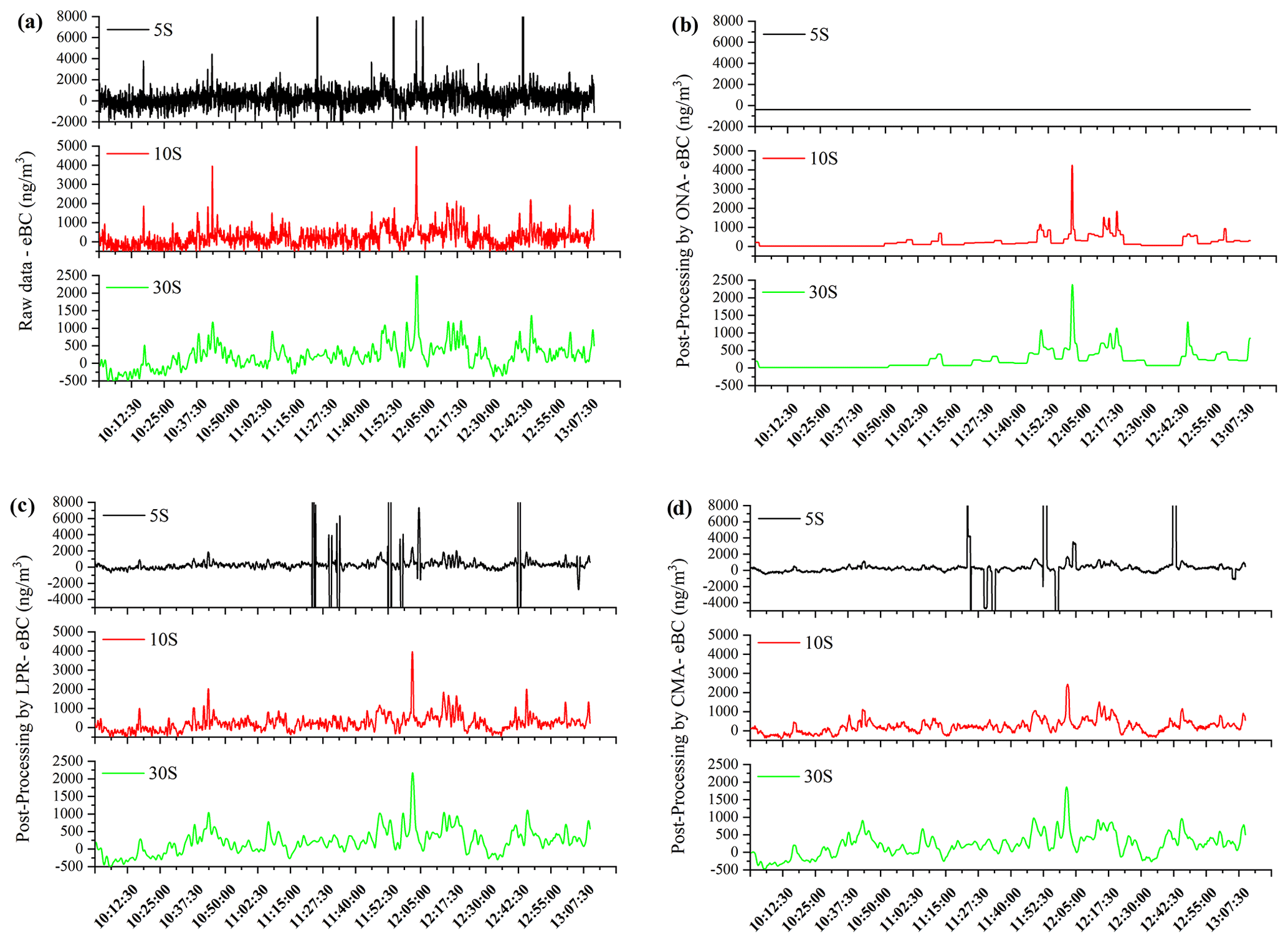
Figure 1The temporal fluctuations of the black carbon levels measured with the MA200 at sampling time bases of 5, 10, and 30 s during a typical sampling period (about 190 min); (a) raw data without noise reduction; (b) data treated with optimized noise reduction averaging; (c) data treated with local polynomial regression; and (d) data treated with centred moving average. The analysis was carried out on data streams from three MA200 devices all collected during a single sampling run (measurements 5, 6, and 7).
Table 2The proportion of negative value (NV) and average reduction of peak (RP) samples under the different post-processing methods (values are shown in percent; NV [%]: proportion of negative values remaining; RP [%]: average reduction of peak samples. Symbol “–” means no data; measurements 1–10).

In the 5 s time base, the eBC values changed very rapidly (Fig. 1a), and the ONA processing of the data resulted in only one value (which was negative) (Fig. 1b). Thus, the microenvironmental characteristics of the eBC concentration were not reproduced. We found that all ΔATN (ATN–ATN0) data were negative in the raw data collected at 5 s, which, according to the ONA method described above, resulted in only a single value. In short, after the first measurement, the ΔATN threshold (which is positive) for calculating the next value was never reached. The first value was likely a negative value due to a combination of instrument noise, coincidence, and a low background concentration (i.e., low baseline instrument signal), which is consistent with both the raw data measurements and the typical low eBC concentrations in the city centre of Augsburg, Germany (Gu, 2012). It is unclear why ΔATN remained negative, but, given the long series of low concentration vales at the beginning of the sampling and the initial negative measurement, it is possible that the summed ΔATN became increasingly negative as a result of the initial negative ΔATN measurement. The subsequent measurements at low concentration did not exceed the magnitude of the initial negative ΔATN value. Under these conditions, a cumulative negative sum of ΔATN would prevent the positive ΔATN threshold from being achieved at all. If true, this condition highlights one potential weakness of the ONA algorithm, such as difficulty registering a signal under low concentrations, and requires further investigation of the conditions under which ONA is truly unbiased. The observed event prevented the use of ONA in the 5 s time base (Fig. 1b). Previous studies in which ONA was successfully applied implemented a 1 s time base (Hagler et al., 2011; Van den Bossche et al., 2015). After post-processing with LPR and CMA, the microenvironmental characteristics retained more detailed information on the eBC concentration. Further comparison of their negative values revealed that the remaining negative values comprised 28.1 % and 22.9 % of the dataset for LPR and CMA, respectively, after post-processing.
In the 10 s interval time base, negative values were not found after ONA processing, suggesting that a reasonable smoothing effect is obtained at low black carbon concentration. The microenvironmental characteristics presented strong changes compared to the raw data, leaving less detailed information on air pollution. After post-processing with LPR and CMA, the microenvironmental characteristics revealed more detailed information on air pollution, with 30.2 % of negative values for LPR and 25.3 % for CMA. In the 30 s interval time base, the negative values comprised 0 % of the post-processed data for ONA, 25.5 % for LPR, and 22.4 % for CMA. The 30 s interval dataset presented the lowest proportion of negative values before and after post-processing, due to the longer interval time of sampling. However, the longer 30 s measurement period results in more distance covered during each measurement, given the mobile nature of the sampling device. Thus, 30 s black carbon measurements may be too long to detect local concentration peaks in urban contexts that supported another study (Kerckhoffs et al., 2016).
The ONA algorithm showed a strong tendency to remove negative values and, depending on the ΔATN threshold employed by the user, can remove potentially meaningful low peaks. As a result, the ONA-treated data may present a bias that obscures nuanced microenvironmental trends (Fig. 1b). Interestingly, LPR and CMA post-processing are capable of decreasing negative values while retaining microenvironmental trends. Both methods are promising for the analysis of spatio-temporal changes in pollutant concentrations with sensitivity to local sources. Previous studies have shown that the spatio-temporal variability of black carbon is highly heterogeneous (Liu et al., 2019, 2021); the ability to capture spatio-temporal variability of microenvironments is critical for assessing differential exposures among populations.
3.2 Reduction and number of peak samples after post-processing methods
The processing of peak sample is a pivotal evaluation index for the measurement of time-averaged roadside air quality. Passing vehicles, for example, may bias estimates of typical local concentrations due to their contribution to the dataset of peak concentrations that may substantially relate to arithmetic averages. Therefore, after noise reduction, we compare the reduction and the retained number of peak samples to further evaluate the post-processing methods.
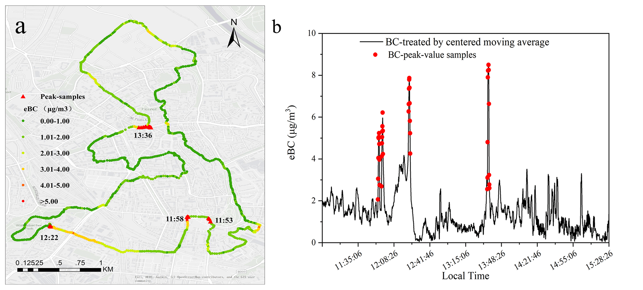
Figure 2Identification of the spatial (a) and temporal (b) distribution characteristics of black carbon peak samples based on the coefficient of variation method (the analysis based on measurement 4); © OpenStreetMap contributors 2020. Distributed under the Open Data Commons Open Database License (ODbL) v1.0.
In the interval time 5 s, the average reduction of peak samples (RP) for the LPR and CMA algorithms was 72.0 % and 87.4 %, respectively (as discussed above, the ONA method could not be used). In this interval time, the reduction of peak samples was relatively high, indicating that when monitoring black carbon at low concentrations and high sample frequencies, drastic noise may occur in the raw data, and higher noise reduction may affect the actual values. Therefore, a suitable interval time should be considered when monitoring low eBC concentrations. In the interval time 10 s, the average reduction of peak samples for CMA (47.7 %) is higher than ONA (5.54 %) and LPR (22.7 %). In the interval time 30 s, CMA presented the greatest average reduction of peak samples (39.1 %) compared to ONA (6.24 %) and LPR (0.62 %) (Table 2, Fig. S4b). The retention of peak samples remaining after post-processing was also assessed using the COV method (measurements 1–10). The result showed that all three algorithms retained all peak samples before and after post-processing. In this regard, CMA retained all peak samples despite the highest reduction in their magnitude. Therefore, CMA highlights microenvironmental trends while preserving the identity of peak samples, facilitating the identification of local pollution sources, and may thus be a better post-processing method than ONA or LPR (Table 2, Fig. S4b).
To further characterize the distribution of peak sample concentration under CMA, we performed an intensive graphical analysis on a single data stream (measurement 4; Fig. 2). As shown in Fig. 2, eBC values along the main roads and intersections were higher than other locations, presumably due in large part to stop-and-go traffic and cars in close proximity to the mobile monitor (Fig. 2). It can be seen from Fig. 2a that the peak samples of black carbon were mainly found in four locations, represented by red triangles. Vehicle counts and traffic in these locations vary depending on the time of measurement. The highest eBC values were repeatedly found in the streets with moderately high traffic volumes and dense coverage with relatively high buildings (street canyon situation), indicating that heterogeneity in air pollution concentrations in Augsburg and similar settings is largely caused by a combination of effects from traffic and topography (Buonanno et al., 2011). To determine whether peak samples are due to local sources or instrumental artefacts and to provide further evidence that traffic and topography effects are primary contributors to spatial heterogeneity in pollution concentrations, we compared the data measurements of the three co-located MA200 units during measurements 5, 6, and 7. The results showed that there were no major differences in the hotspot areas (an indicator of considerable peak samples) identified by the measurements of the three instruments (Fig. S5).
3.3 Comparison of background estimation and correction after noise reduction
Local air pollution can be highly affected by long-range and regional transport. The timing and magnitude of such transport events vary in space and time and are highly dependent upon the stochasticity of meteorology. As a result, local background concentration changes may vary, affecting the comparability of measurements made at the same location at different times (Brantley et al., 2014). For this reason, reliable comparison of time-variable mobile measurements across a city (and thus reliable pinpointing of hotspots and pinpointing of key local sources) requires effective methods to estimate, isolate, and remove the effects of fluctuations in background concentration. Our analysis indicates that the effectiveness of background correction is affected by the noise reduction method chosen during post-processing.
After post-processing, the data were evaluated using the TPRS method. We calculated the 5 and 10 min background concentrations under different post-processing approaches. As shown in Fig. 3a and b, the background concentration after LPR processing has both the largest proportion of negative values and the most negative values (i.e., negative values of the greatest absolute magnitude), resulting in estimates of background-corrected concentrations that are greater than actual monitored concentrations. Background concentrations calculated after ONA and CMA post-processing presented fewer and lower negative values than LPR but were not convincingly different from each other. Therefore, to further compare the ONA and CMA algorithms, we also compared concentrations after background correction (Fig. 3c and d). As shown in Fig. 3c and d, when the concentration is lower than 1 µg/m3, the background-corrected results after the ONA processing are smoother than after CMA. This result dampens the signal of local pollutant sources, resulting in a lower utility of post-processed data.
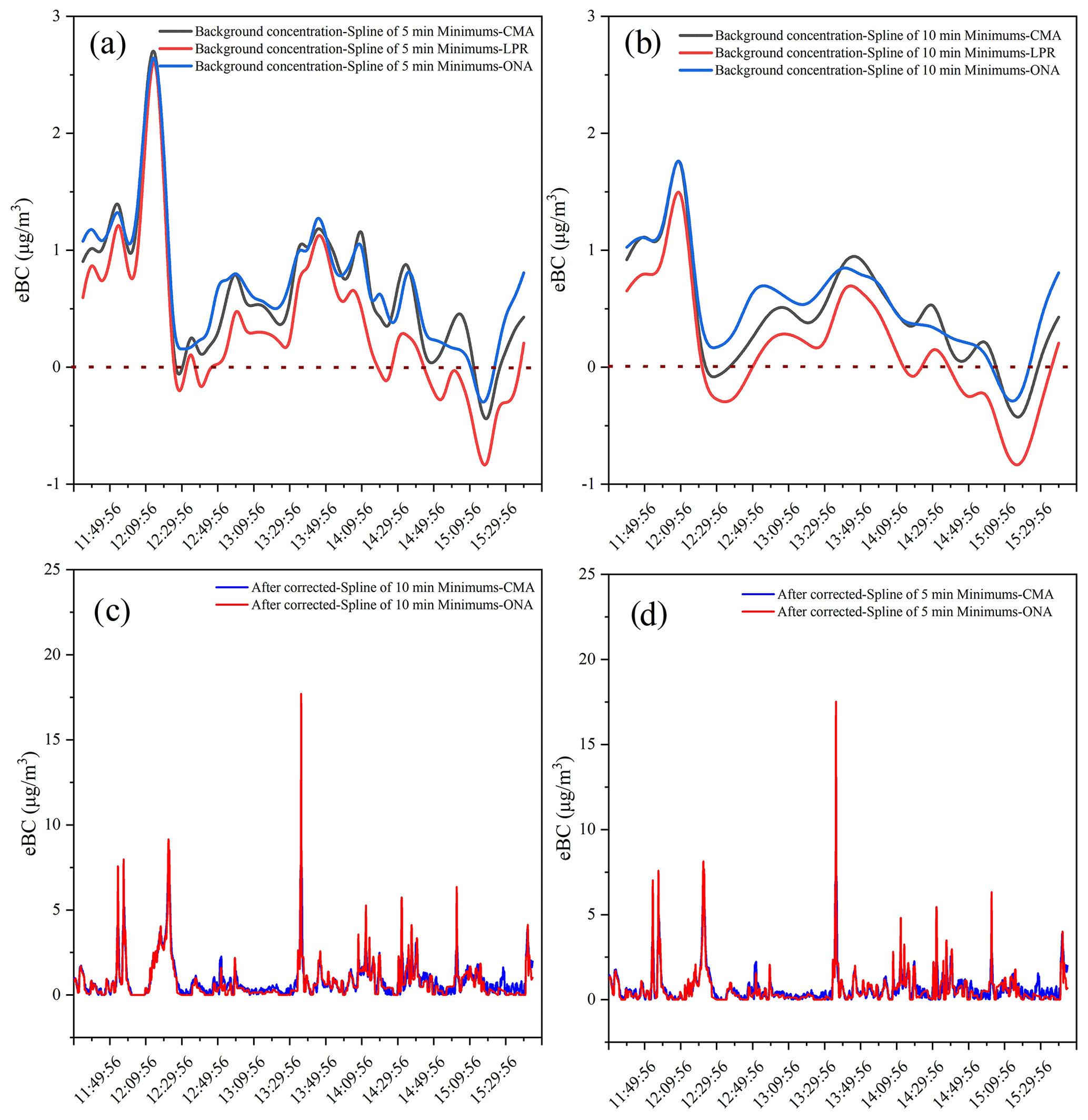
Figure 3Background concentration of black carbon under different time series for (a) spline of 5 min minimums and (b) spline of 10 min minimums and after being corrected for (c) spline of 5 min minimums and (d) spline of 10 min minimums. Analyses are based on measurement 4.
In order to verify the CMA applicability and its advantages, this study further analysed the eBC concentrations measured by a fixed background monitoring station at the University of Applied Sciences (UAS) (Fig. S6) (Cyrys et al., 2006). The background value under the 5 min window exhibits wave-like characteristics, and the fitting curve in the 10 min window is relatively smooth. However, the TPRS-based background value often does not fluctuate greatly over short periods, and the black carbon background value curve under the 5 min window does not conform to the “actual” urban background situation as estimated using the fixed-site monitor data, which are assumed to primarily represent the fluctuations in background concentrations. Moreover, by comparing the curve produced by the spline of 10 min minimums with the eBC background concentration (“Background-UAS”, Fig. S6), it can be found that the background correction method based on the time series can well characterize the time-varying characteristics of background pollution in each experiment, suggesting that, of the two options, 10 min showed the better window for fitting the background value curve of black carbon.
Under the TPRS method, the background concentration of eBC can be fitted at any sampling time. The TPRS-estimated background contribution of the observed eBC concentration averaged 37.8 % of the total measured concentration. However, when the contribution of background concentration to a single measurement was examined, a large fluctuation (10.4 %–71.3 %) was observed, which may be closely related to sizable changes in the meteorological conditions, traffic conditions along the road (and over time at the same point in the road), and urban street canyon effects in each measurement. Therefore, based on the comparison of background correction, CMA showed better applications for estimating the background concentration and location source contribution.
3.4 Generalizability
To verify the generalizability of our assessment, we performed another three measurement runs in Munich (measurements 8, 9, and 10). Raw data were post-processed for noise reduction using CMA (Fig. S7). The results showed that the following method is equally applicable in a city like Munich as in our study site in Augsburg, which are two cities that differ in location and environmental characteristics (e.g., population, economy, traffic density, etc.). After treated using CMA, the peak samples can be identified in different interval times (Fig. S8), and the estimated background concentrations showed few negative values (Fig. S9). Further research into the transferability of our results to a more diverse set of contexts is still needed.
3.5 Practical implications
The MA200 is widely used to measure human exposure to black carbon and for mobile air quality monitoring. In this study the MA200 devices were applied in mobile measurements in an urban area (Augsburg), and the sensitivity of the final analysis to various data post-processing methods was investigated. In contrast to our findings, Hagler et al. (2011) suggested the use of the ONA algorithm to post-process Aethalometer data from microAeth AE51, portable AE42, and rack-mounted AE21 Aethalometer instruments (Magee Scientific, Berkeley, CA, USA). In their analysis, ONA demonstrated a strong noise reduction in all datasets and retained spatio-temporal variation. ONA also reduced the occurrence of negative data values in low concentration sampling environments. However, for the microAeth® series of black carbon monitoring instruments, our study showed that ONA under reasonable ΔATN thresholding may lead to a considerable dampening of spatio-temporal resolution in local black carbon signals at street level – an effect that is lower under CMA post-processing.
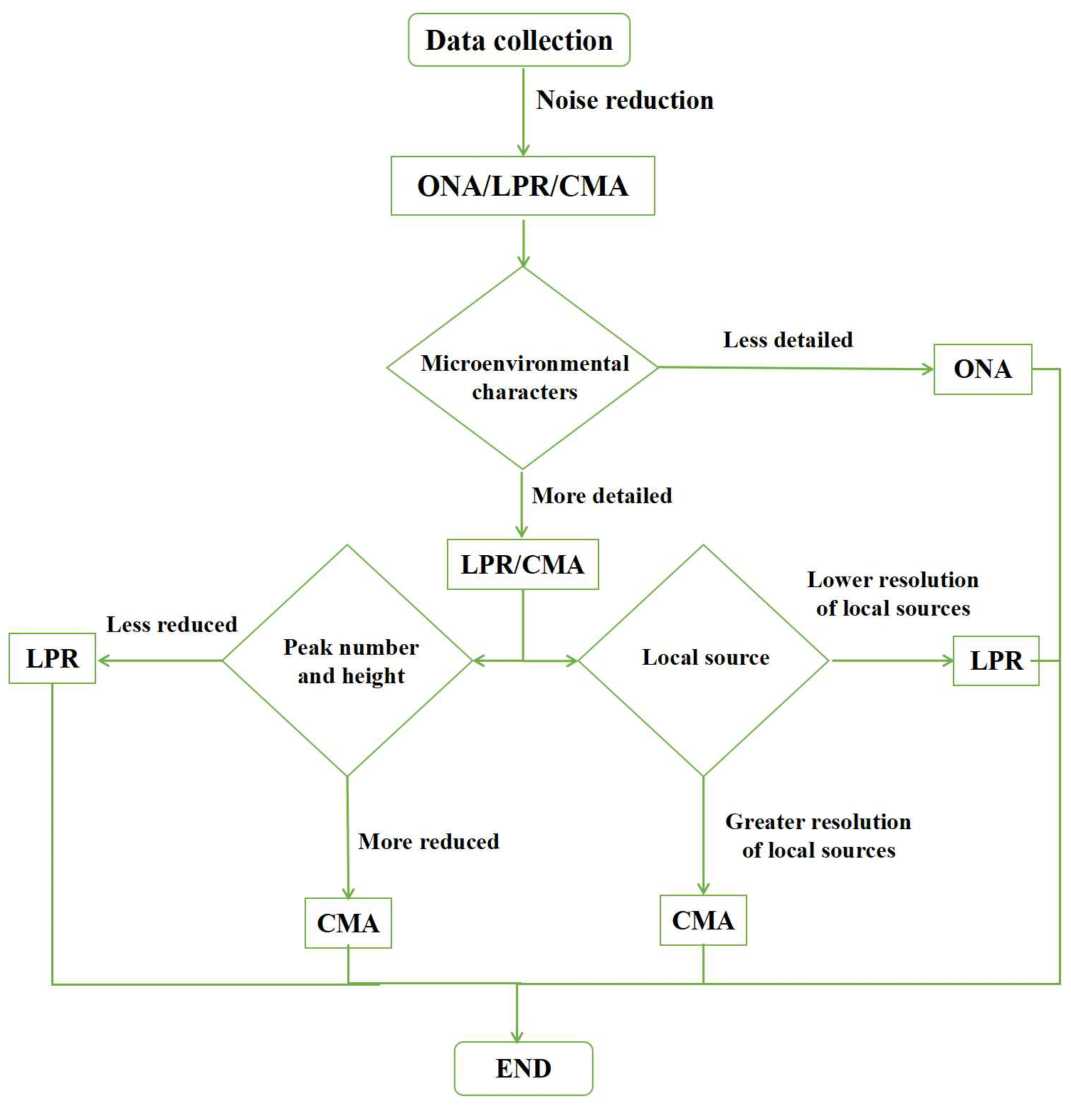
In addition, our analysis highlights that the selection of an appropriate data post-processing method is crucial to the proper assessment and interpretation of exposure-relevant microenvironmental contributors to pollution concentrations in urban areas. This analysis is important when estimating exposures that occur during transit, where spatio-temporal variability in pollution concentrations is vast, like in commuter traffic (Snyder et al., 2013). Due to the typically low-but-heterogeneous nature of eBC concentrations in many areas like Augsburg, noisy measurement with the MA200 under high-frequency sampling may obscure actual trends in measured values. This study demonstrated that post-processing MA200 data using CMA can reliably extract the actual signals from such noise and, alternatively, that post-processing via ONA and LPR could be less reliable. Future researchers and agencies may find a distillation of our results in the form of the flow diagram in Scheme 1 useful in determining how to reliably assess spatio-temporal variability of MA200 measurements for black carbon in different microenvironments.
A mobile monitoring campaign was conducted in the city centre of Augsburg, Germany, to determine a suitable noise reduction algorithm for the MA200 Aethalometer. Our results showed that, at the interval times of 5, 10, and 30 s, CMA post-processing effectively removed spurious negative concentrations without major bias and reliably highlighted effects from local sources, effectively increasing spatio-temporal resolution in mobile measurements. Evaluation of the effects of each method on peak sample reduction and the estimation of background concentrations further support the reliability of CMA. Further analysis is needed to understand how well these findings apply in different seasons; across different diurnal patterns; and in more rural, more urban, and non-German locations.
The data are available upon request by contacting the first author of the paper (xiansheng.liu@helmholtz-muenchen.de).
The supplement related to this article is available online at: https://doi.org/10.5194/amt-14-5139-2021-supplement.
XL was responsible for data curation, methodology and software analysis, and writing original draft. HH was responsible for methodology, software analysis, and writing original draft. XZ was responsible for funding acquisition and project administration. LDH was responsible for discussion and review and editing. JSK was responsible for investigation and supervision. JB and GJ were responsible for methodology. AHAW and BSH were responsible for writing, review and editing. RZ was responsible for investigation.
L. Drew Hill is an employee of AethLabs (San Francisco, CA, USA) and Andrew H. A. White was, at the time of contribution, an intern at AethLabs. These affiliations did not affect the conclusions of the paper.
Publisher’s note: Copernicus Publications remains neutral with regard to jurisdictional claims in published maps and institutional affiliations.
We gratefully thank Erik Hopp (AethLabs, San Francisco, CA, USA) for the implementation and maintenance of the AethLabs data processing web tool.
The work is funded by the National Key Research and Development Program of China (grant no. 2020YFB1806500), Support Project of High-level Teachers in Beijing Municipal Universities in the Period of 13th Five-year Plan (grant no. CIT&TCD201904037), the National Natural Science Foundation of China (grant no. 81800854), and the Germany Federal Ministry of Transport and Digital Infrastructure (BMVI) as part of SmartAQnet (grant no. 19F2003B).
This paper was edited by Alfred Wiedensohler and reviewed by two anonymous referees.
AethLabs: MicroAeth® MA Series MA200, MA300, MA350 Operating Manual, available at: https://aethlabs.com/sites/all/content/microaeth/maX/MA200 MA300 MA350 Operating Manual Rev 03 Dec 2018.pdf (last access: 5 April 2021), 2018.
Anenberg, S. C., Schwartz, J., Shindell, D., Amann, M., Faluvegi, G., Klimont, Z., Janssens-Maenhout, G., Pozzoli, L., Dingenen., R. V., Vignati, E., Emberson, L., Muller, N. Z., West, J. J., Williams, M., Demkine, M., Demkine, V., Hicks, W. K., Kuylenstierna, J., Raes, F., and Ramanathan, V.: Global air quality and health co-benefits of mitigating near-term climate change through methane and black carbon emission controls, Environ. Health Persp., 120, 831–839, https://doi.org/10.1289/ehp.1104301, 2012.
Apte, J. S., Kirchstetter, T. W., Reich, A. H., Deshpande, S. J., Kaushik, G. C. A., Marshall, J, D., and Nazaroff, W. W.: Concentrations of fine, ultrafine, and black carbon particles in auto-rickshaws in New Delhi, India, Atmos. Environ., 45, 4470–4480, https://doi.org/10.1016/j.atmosenv.2011.05.028, 2011.
Apte, J. S., Messier, K. P., Gani, S., Brauer, M., Kirchstetter, T. W., Lunden, M. M., Maeshall, J. D., Portier, C. J., Vermeulen, R. C. H., and Hameurg, S. P.: High-Resolution Air Pollution Mapping with Google Street View Cars. Exploiting Big Data, Environ. Sci. Technol., 12, 6999–7008, https://doi.org/10.1021/acs.est.7b00891, 2017.
Brantley, H. L., Hagler, G. S. W., Kimbrough, E. S., Williams, R. W., Mukerjee, S., and Neas, L. M.: Mobile air monitoring data-processing strategies and effects on spatial air pollution trends, Atmos. Meas. Tech., 7, 2169–2183, https://doi.org/10.5194/amt-7-2169-2014, 2014.
Breidt, F. J. and Opsomer. J. D.: Local polynomial regression estimators in survey sampling, Ann. Stat., 28, 1026–1053, available at: https://www.jstor.org/stable/2673953 (last access: 22 November 2020), 2000.
Buonanno, G., Fuoco, F. C., and Stabile, L.: Influential parameters on particle exposure of pedestrians in urban microenvironments, Atmos. Environ., 7, 1434–1443, https://doi.org/10.1016/j.atmosenv.2010.12.015, 2011.
Cai, J., Yan, B., Kinney, P. L., Perzanowski, M. S., Jung, K. H., Li, T., Xiu, G., Zhang, D., Olivo, C., Ross, J., Miller, R. L., and Chillrud, S. N.: Optimization approaches to ameliorate humidity and vibration related issues using the microAeth black carbon monitor for personal exposure measurement, Aerosol Sci. Tech., 47, 1196–1204, https://doi.org/10.1080/02786826.2013.829551, 2013.
Cao, R., Li, B., Wang, H. W., Tao, S., Peng, Z. R., and He, H. D.: Vertical and Horizontal Profiles of Particulate Matter and Black Carbon Near Elevated Highways Based on Unmanned Aerial Vehicle Monitoring, Sustainability, 12, 1204, https://doi.org/10.3390/su12031204, 2020.
Cheng, Y. H. and Lin, M. H.: Real-time performance of the microAeth® AE51 and the effects of aerosol loading on its measurement results at a traffic site. Aerosol Air Qual. Res., 13, 1853–1863, https://doi.org/10.4209/aaqr.2012.12.0371, 2013.
Choi, W., He, M., Barbesant, V., Kozawa, K. H., Mara, S., Winer, A. M., and Paulosn, S. E.: Prevalence of wide area impacts downwind of freeways under pre-sunrise stable atmospheric conditions, Atmos. Environ., 62, 318–327, https://doi.org/10.1016/j.atmosenv.2012.07.084, 2012.
Cyrys, J., Pitz, M., Soentgen, J., Zimmermann, R., Wichmann, H. E., and Peters, A.: New Measurement Site for Physical and Chemical Particle Characterization in Augsburg. Germany, Epidemiology (Cambridge, Mass.), 17, S250–S251, 2006.
Dons, E., Int Panis, L., Van Poppel, M., Theunis, J., and Wets, G.: Personal exposure to Black Carbon in transport microenvironments, Atmos. Environ., 55, 392–398, https://doi.org/10.1016/j.atmosenv.2012.03.020, 2012.
Drewnick, F., Böttger, T., von der Weiden-Reinmüller, S.-L., Zorn, S. R., Klimach, T., Schneider, J., and Borrmann, S.: Design of a mobile aerosol research laboratory and data processing tools for effective stationary and mobile field measurements, Atmos. Meas. Tech., 5, 1443–1457, https://doi.org/10.5194/amt-5-1443-2012, 2012.
Easton, V. J. and McColl, J. H.: Statistics Glossary v1.1, available at: http://www.stats.gla.ac.uk/steps/glossary/index.html, (last access: 22 November 2020), 1997.
Goldberg, E. D.: Black carbon in the environment: properties and distribution, J. Wiley, available at: https://agris.fao.org/agris-search/search.do?recordID=US880866588 (last access: 22 November 2020), ISBN 04-718-19794, 1985.
Gu, J.: Characterizations and sources of ambient particles in Augsburg. Germany, available at: https://opus.bibliothek.uni-augsburg.de/opus4/2103, (last access: 22 November 2020), 2012.
Hagler, G. S., Yelverton, T. L., Vedantham, R., Hansen, A. D., and Turner, J. R.: Post-processing Method to Reduce Noise while Preserving High Time Resolution in Aethalometer Real-time Black Carbon Data, Aerosol Air Qual. Res., 11, 539–546, https://doi.org/10.4209/aaqr.2011.05.0055, 2011.
Hagler, G. S. W., Lin, M., Khlystov, A., Baldauf, R. W., Isakov, V., Faircloth, J., and Jackson, L. E.: Field investigation of roadside vegetative and structural barrier impact on near-road ultrafine particle concentrations under a variety of wind conditions, Sci. Total Environ., 416, 7–15, https://doi.org/10.1016/j.scitotenv.2011.12.002, 2012.
Janssen, N. A., Hoek, G., Simic-Lawson, M., Fischer, P., Van Bree, L., Ten Brink, H., Keuken, M., Atkinson, R. W., Anderson, H. R., Brunekreef, B., and Cassee, F. R.: Black carbon as an additional indicator of the adverse health effects of airborne particles compared with PM10 and PM2.5, Environ. Health Persp., 119, 1691–1699, https://doi.org/10.1289/ehp.1003369, 2011.
Kai, B., Li, R., and Zou, H.: Local composite quantile regression smoothing: an efficient and safe alternative to local polynomial regression, J. Roy. Stat. Soc. B, 72, 49–69, https://doi.org/10.1111/j.1467-9868.2009.00725.x, 2010.
Kerckhoffs, J., Hoek, G., Messier, K. P., Brunekreef, B., Meliefste, K., Klompmaker, J. O., and Vermeulen, R.: Comparison of ultrafine particle and black carbon concentration predictions from a mobile and short-term stationary land-use regression model, Environ. Sci. Technol., 50, 12894–12902, https://doi.org/10.1021/acs.est.6b03476, 2016.
Kutzner, R. D., von Schneidemesser, E., Kuik, F., Queddenau, J., Weatherhead, E. C., and Schamle, J.: Long-term monitoring of black carbon across Germany, Atmos. Environ., 185, 41–52, https://doi.org/10.1016/j.atmosenv.2018.04.039, 2018.
Liu, M., Peng, X., Meng, Z., Zhou, T., Long, L., and She, Q.: Spatial characteristics and determinants of in-traffic black carbon in Shanghai, China: Combination of mobile monitoring and land use regression model, Sci. Total Environ., 658, 51–61, https://doi.org/10.1016/j.scitotenv.2018.12.135, 2019.
Liu, X., Schnelle-Kreis, J., Zhang, X., Bendl, J., Khedr, M., Jakobi, G., Schloter-Hai, B., Hovorka, J., and Zimmermann, R.: Integration of air pollution data collected by mobile measurement to derive a preliminary spatiotemporal air pollution profile from two neighboring German-Czech border villages, Sci. Total Environ., 722, 137632, https://doi.org/10.1016/j.scitotenv.2020.137632, 2020.
Liu, X., Zhang, X., Schnelle-Kreis, J., Jakobi, G., Cao, X., Cyrys, J., Yang, L., Schloter-Hai, B., Abbaszade, G., Orasche, J., Khedr, M., Kowalski, M., Hank., M., and Ralf Zimmermann, R.: Spatiotemporal Characteristics and Driving Factors of Black Carbon in Augsburg, Germany: Combination of Mobile Monitoring and Street View Images, Environ. Sci. Technol., 55, 160–168, https://doi.org/10.1021/acs.est.0c04776, 2021.
Masry, E.: Multivariate local polynomial regression for time series: uniform strong consistency and rates, J. Time Ser. Anal., 17, 571–599, https://doi.org/10.1111/j.1467-9892.1996.tb00294.x, 1996.
Nichols, J. L., Owens, E. O., Dutton, S. J., and Luben, T. J.: Systematic review of the effects of black carbon on cardiovascular disease among individuals with pre-existing disease, Int. J. Public Health, 58, 707–724, https://doi.org/10.1007/s00038-013-0492-z, 2013.
Sadiq, M., Tao, W., Tao, S., and Liu, J.: Air quality and climate responses to anthropogenic black carbon emission changes from East Asia, North America and Europe, Atmos. Environ., 120, 262–276, https://doi.org/10.1016/j.atmosenv.2015.07.001, 2015.
Snyder, E. G., Watkins, T. H., Solomon, P. A., Thoma, E. D., Williams, R. W., Hagler, G. S., Shelow, D., Hindin, D. A., Kilaru, V. J., and Preuss, P. W.: The changing paradigm of air pollution monitoring, Environ. Sci. Technol., 47, 11369–11377, https://doi.org/10.1021/es4022602, 2013.
Van den Bossche, J., Peters, J., Verwaeren, J., Botteldooren, D., Theunis, J., and De Baets, B.: Mobile monitoring for mapping spatial variation in urban air quality: Development and validation of a methodology based on an extensive dataset, Atmos. Environ., 105, 148–161, https://doi.org/10.1016/j.atmosenv.2015.01.017, 2015.
Virkkula, A., Mäkelä, T., Hillamo, R., Yli-Tuomi, T., Hirsikko, A., Hämeri, K., and Koponen, I. K.: A simple procedure for correcting loading effects of aethalometer data, J. Air. Waste Manage., 57, 1214–1222, https://doi.org/10.3155/1047-3289.57.10.1214, 2007.
Wang, Z., Lu, F., He, H., Lu, Q., Wang, D., and Peng, Z.: Fine-scale estimation of carbon monoxide and fine particulate matter concentrations in proximity to a road intersection by using wavelet neural network with genetic algorithm, Atmos. Environ., 104, 264–272, https://doi.org/10.1016/j.atmosenv.2014.12.058, 2015.
Zhou, H., Lin, J., Shen, Y., Deng, F., Gao, Y., Liu, Y., Dong, H., Zhang, Y., Sun, Q., Fang, J., Tang, S., Wang, Y., Du, Y., Cui, L., Ruan, S., Kong, F., Liu, Z., and Li, T.: Personal black carbon exposure and its determinants among elderly adults in urban China, Environ. Int., 138, 105607, https://doi.org/10.1016/j.envint.2020.105607, 2020.