the Creative Commons Attribution 4.0 License.
the Creative Commons Attribution 4.0 License.
 | 30 Jul 2021
Evaluation of the coupled high-resolution atmospheric chemistry model system MECO(n) using in situ and MAX-DOAS NO2 measurements
Julia Remmers
Steffen Beirle
Joachim Fallmann
Astrid Kerkweg
Jos Lelieveld
Mariano Mertens
Andrea Pozzer
Benedikt Steil
Marc Barra
Holger Tost
Thomas Wagner
We present high spatial resolution (up to 2.2×2.2 km2) simulations focussed over south-west Germany using the online coupled regional atmospheric chemistry model system MECO(n) (MESSy-fied ECHAM and COSMO models nested n times). Numerical simulation of nitrogen dioxide (NO2) surface volume mixing ratios (VMRs) are compared to in situ measurements from a network with 193 locations including background, traffic-adjacent and industrial stations to investigate the model's performance in simulating the spatial and temporal variability of short-lived chemical species. We show that the use of a high-resolution and up-to-date emission inventory is crucial for reproducing the spatial variability and resulted in good agreement with the measured VMRs at the background and industrial locations with an overall bias of less than 10 %. We introduce a computationally efficient approach that simulates diurnal and daily variability in monthly-resolved anthropogenic emissions to resolve the temporal variability of NO2.
MAX-DOAS (Multiple AXis Differential Optical Absorption Spectroscopy) measurements performed at Mainz (49.99∘ N, 8.23∘ E) were used to evaluate the simulated tropospheric vertical column densities (VCDs) of NO2. We propose a consistent and robust approach to evaluate the vertical distribution of NO2 in the boundary layer by comparing the individual differential slant column densities (dSCDs) at various elevation angles. This approach considers details of the spatial heterogeneity and sensitivity volume of the MAX-DOAS measurements while comparing the measured and simulated dSCDs. The effects of clouds on the agreement between MAX-DOAS measurements and simulations have also been investigated. For low elevation angles (≤8∘), small biases in the range of −14 % to +7 % and Pearson correlation coefficients in the range of 0.5 to 0.8 were achieved for different azimuth directions in the cloud-free cases, indicating good model performance in the layers close to the surface. Accounting for diurnal and daily variability in the monthly-resolved anthropogenic emissions was found to be crucial for the accurate representation of time series of measured NO2 VMR and dSCDs and is particularly critical when vertical mixing is suppressed, and the atmospheric lifetime of NO2 is relatively long.
- Article
(16403 KB) - Full-text XML
- BibTeX
- EndNote


Regional atmospheric chemistry and transport models are important for the study and forecasting of atmospheric processes at fine spatial resolutions. The high spatial resolution of these models allows us to resolve localized emissions (e.g. industrial and urban clusters) and quantify their impacts on non-linear photochemical processes, e.g. ozone production (Vinken et al., 2014; Visser et al., 2019; Mertens et al., 2020a) as well as on heterogeneous processes, e.g. particulate nitrate production (Chen et al., 2020). Various studies have shown that significant improvements in satellite retrievals can be achieved through the incorporation of highly resolved a priori trace gas and aerosol fields calculated by high-resolution regional models (Valin et al., 2011; Liu et al., 2020; Ialongo et al., 2020).
Regional models achieve high resolution by employing nesting around the location of interest, in which a fine-resolution model domain receives meteorological and chemical boundary conditions from a coarser resolution model spanning a broader area. The MECO(n) (MESSy-fied ECHAM and COSMO models nested n times) regional model system developed by Kerkweg and Jöckel (2012b) allows for online coupling between different nests and in this way facilitates frequent updates of meteorological and chemical boundary conditions. The use of MESSy submodels for this coupled system also ensures consistent treatment of chemical speciation, chemistry and several other relevant processes governing the concentration of chemical species among various nests. A chemical evaluation of MECO(n) over Europe was performed by Mertens et al. (2016) for a set-up at km2 spatial resolution for nitrogen dioxide (NO2), ozone (O3) and carbon monoxide (CO). The main strength of MECO(n), i.e. the online coupling with the COSMO model, makes it suitable for performing very high resolution (e.g. km2) simulations. For example, the operational COSMO model is already being used for weather forecasts at a spatial resolution of 2.8×2.8 km2 by the German Meteorological Service (Deutscher Wetterdienst) and at 1×1 km2 by the Federal Office of Meteorology and Climatology, Switzerland (MeteoSwiss). Similar high-resolution model simulations including chemistry have been shown to better represent local maxima (e.g. isolated point sources, road networks and ship tracks) and facilitate understanding of sector-specific impacts on secondary pollution (e.g. ozone production) (Colette et al., 2014; Mertens et al., 2020a). However, comparison with in situ measurements showed that these gains could only be quantitatively determined up to a resolution of km2, beyond which major improvements were not observed (Colette et al., 2014). In most of the cases, the improvement was limited by the resolution of the input emission inventory used in these studies, which are available at a much coarser resolution than that of the model set-up. Apart from the coarse resolution, further limitations in such comparisons are imposed by the availability of mostly outdated anthropogenic emissions inventory and limited information about short-term temporal variability (e.g. day of the week or hour of the day) (Kuik et al., 2018). In most cases, input emission inventories are available at temporal resolutions of months to years, but in reality, emissions from several sectors (e.g. road transport, residential combustion) vary markedly depending on the hour of the day and day of the week. From a modelling perspective, however, incorporating high temporal resolution input emissions can be computationally inefficient due to the high readout time and subsequent requirement for interpolation on the model grid.
The evaluation of high-resolution mesoscale models is even more challenging due to the limited availability (in situ measurements) and unavailability (e.g. satellite observations) of reference datasets. TROPOMI (TROPOspheric Monitoring Instrument) aboard the Sentinel-5P satellite (Veefkind et al., 2012) has a high spatial resolution (up to 3.5×5.5 km2) and is in principle well suited for comparison of the tropospheric vertical column densities (VCDs) simulated by the model. However, the limited temporal information – generally measurements from one overpass per day – precludes an evaluation of diurnal profiles; hence, TROPOMI is not well suited to demonstrating the advantages of considering diurnally varying input emissions. Besides VCDs, conventional model evaluation studies are often restricted to the evaluation of concentrations at discrete layers (most often at the surface) using in situ measurements which are limited with respect to the temporal and spatial coverage. Evaluations of model vertical profiles are even rarer due to the paucity of vertically resolved measurements (e.g. balloon-based and aircraft measurements), which are technically very challenging. For example, discrepancies between regional models (WRF-Chem and CHIMERE) and measurements were proposed to arise due to inappropriate parametrization of the turbulent diffusion constant; however, this could not be verified due to the lack of vertically resolved NO2 measurements (Kuik et al., 2018; Schaap et al., 2015). Mertens et al. (2016) evaluated the vertical profiles of O3 simulated by MECO(n) using ozone-sonde data, but this provides little information about the variability within the boundary layer which is masked by that in the upper troposphere (above 400 hPa or ≈7 km).
In this regard, MAX-DOAS (Multiple AXis Differential Optical Absorption Spectroscopy) measurements (Hönninger et al., 2004) provide a unique opportunity for model evaluation for a larger representative area (a few square kilometres) and over long temporal scales. To our knowledge, regional model comparison studies with MAX-DOAS are very limited (e.g. Shaiganfar et al., 2015; Vlemmix et al., 2015; Blechschmidt et al., 2020) and mostly focus on the tropospheric VCDs. These studies have shown moderate correlations between MAX-DOAS and regional model calculated VCDs with major differences arising due to inappropriate representation of anthropogenic emissions, differences between model-simulated and actual wind vectors, the presence of clouds, and uncertainties related to the MAX-DOAS VCD retrieval. Further limitations in these comparisons arise due to assumptions of horizontal homogeneity and the challenges associated with accurately defining the area/volume for which the MAX-DOAS measurements are sensitive. In addition to the VCDs, there is additional information content in the MAX-DOAS measurements (e.g. spatial distribution of trace gases), which comes from scans performed at different elevation angles, thus probing the atmosphere along different light paths. This information can be utilized to evaluate the performance of regional models in accurately simulating the spatial distribution within the boundary layer.
In this paper, we present high-resolution (up to 2.2×2.2 km2) MECO(3) simulations of NO2 over south-west Germany using a high spatial resolution and up-to-date input emission inventory. We also effectively account for the day-of-the-week and diurnal variability in anthropogenic emissions in the model simulations by applying sector-specific hourly scaling factors to the monthly-resolved anthropogenic emissions. The model description, details of MAX-DOAS measurements and analyses as well as other reference data are provided in Sect. 2. We evaluate the model performance with respect to two input emission inventories and temporal resolution of emissions through comparison with in situ measurements in Sect. 3.2 and MAX-DOAS tropospheric NO2 VCDs in Sect. 3.3. The TROPOMI comparison will be the focus of a future study. In this paper, we introduce a sophisticated and consistent approach for MAX-DOAS comparison, which overcomes the limitations of previous such comparisons. We also evaluate the performance of the model in reproducing the vertical distribution of NO2 within the boundary layer.
2.1 Model description
We use the one-way coupled model system MECO(3) (Kerkweg and Jöckel, 2012a, b) based on MESSy version 2.54 (Jöckel et al., 2010), which couples the global chemistry climate model EMAC (Jöckel et al., 2006) one-way to the regional model COSMO-CLM/MESSy (called COSMO/MESSy hereafter). COSMO-CLM is the community model of the German regional climate research community jointly further developed by the CLM-Community (Rockel et al., 2008). The core driving model for EMAC is ECHAM5 version 5.3.02 (Roeckner et al., 2003), and for COSMO/MESSy it is COSMO 5.00_clm10 (Rockel et al., 2008; Steppeler et al., 2003). EMAC is configured with T106L31ECMWF spectral resolution corresponding to a grid resolution of , extending up to 10 hPa (≈30 km over Europe) vertically in 31 vertical layers and time step of 360 s. The global model meteorology (temperature, vorticity, surface pressure and divergence) is nudged to 6-hourly ECMWF ERA-Interim reanalysis data. Model simulations are performed for May 2018, i.e. from 1 May 2018 00:00:00 until 1 June 2018 00:00:00. The initial chemical conditions for the regional model instances are provided by an EMAC simulation starting 3 years before the MECO(n) simulations start, i.e. on 1 March 2015.
The three instances of the COSMO/MESSy model are coupled online one-way from coarser resolution to finer resolution. The first instance of COSMO/MESSy has a spatial resolution of ( km2; referred to as CM50 hereafter), the second one at ( km2; referred to as CM07 hereafter) and the third one at ( km2; referred to as CM02 hereafter). All three COSMO/MESSy domains are set up in a rotated coordinate system with the location of the north pole at 40∘ N and −170∘ E. The CM07 domain is focussed around Germany, and CM02 further zooms in to south-west Germany, as shown in Fig. 1. CM50 and CM07 have 40 terrain-following vertical levels extending up to 22.7 km, while CM02 has 50 terrain-following vertical levels extending up to 22 km. In all the three domains, the lowermost atmospheric model layer has a thickness of 20 m, while the lowest 1 km is split into 11 levels for CM50 and CM07 and 12 levels for CM02. The thickness of the vertical layers increases with altitude. The time steps for CM50, CM07 and CM02 are 120, 60 and 20 s, respectively. The online coupling enables the specification of boundary conditions at each time step by the respective driving model and is particularly advantageous for complex atmospheric chemistry modelling involving hundreds of chemical tracers. Convection is parameterized according to the Tiedtke–Bechtold scheme for both CM50 and CM07 domains, while for the CM02 domain only shallow convection is parameterized according to the Tiedtke scheme (Bechtold et al., 2001; Tiedtke, 1989).
The MECO(n) model set-up achieves a very high consistency within the model chain, as all four model instances (EMAC and three times COSMO/MESSy) use MESSy and thus imply the very same chemical speciation and process formulations for the chemical processes (e.g. online/offline emission of chemical tracers, ONEMIS/OFFEMIS; chemistry, MECCA; dry deposition, DDEP; wet scavenging, SCAV and photolysis, JVAL) (Jöckel et al., 2010; Tost et al., 2006; Kerkweg et al., 2006a; Sander et al., 2014; Kerkweg et al., 2006b). Since deep convection is resolved in the CM02 domain, the MESSy submodel CVTRANS (Tost et al., 2010) used to calculate the tracer transport due to convection is not used in this domain. Consequently, convective scavenging and convective rain flux are also disabled in the CM02 domain when using the SCAV submodel (Tost et al., 2006). For the chemical mechanism in MECCA, we use the Mainz Isoprene Mechanism (MIM 1) (Pöschl et al., 2000), including 142 gaseous chemical species involved in 236 gas and multiphase reactions and 74 photochemical reactions.
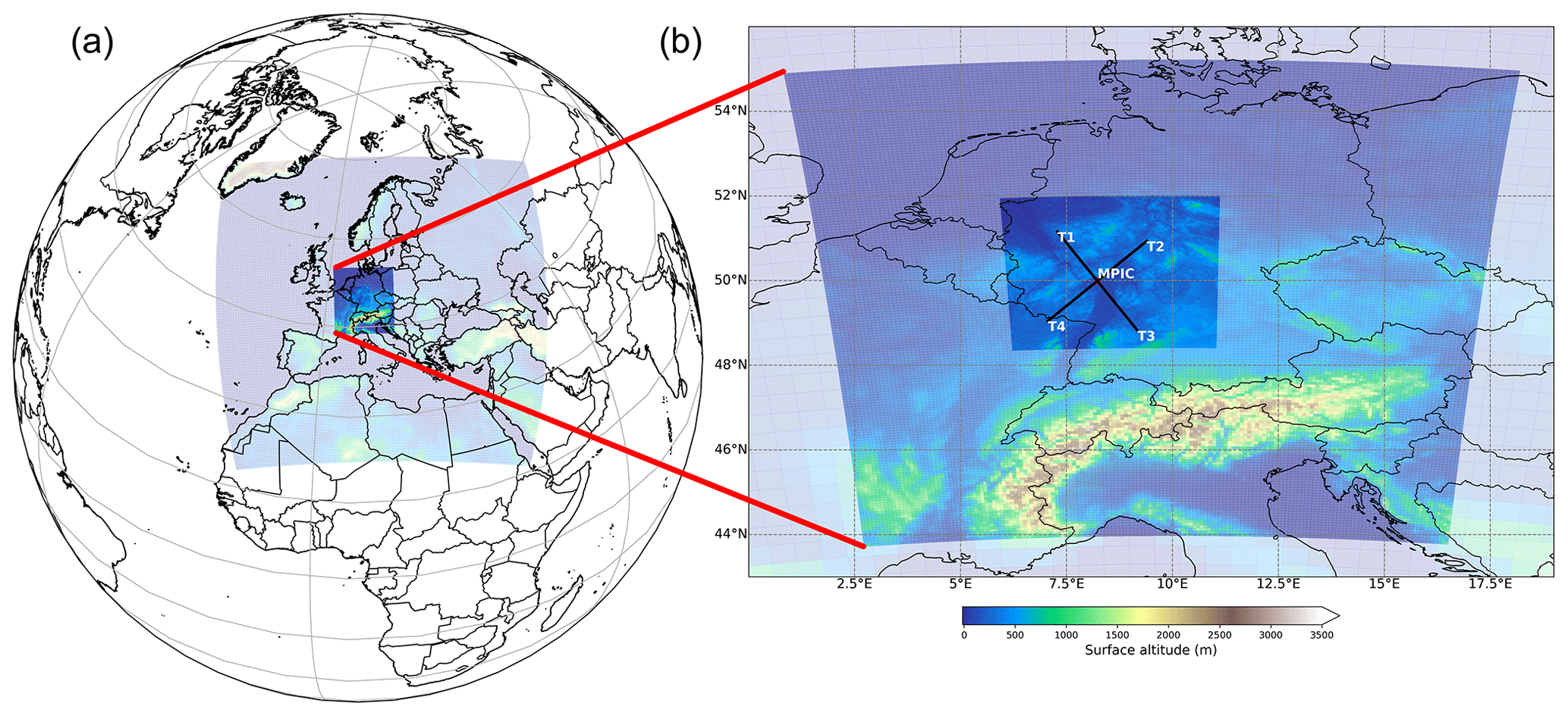
Figure 1MECO(3) domains in panel (a) colour-coded according to the surface altitude. A close-up of the map in the right panel shows the CM07 and CM02 domains. The location of MPIC (Max Planck Institute for Chemistry) is shown as the red dot in panel (b) with the arrows pointing in the viewing direction of the four telescopes.
For the global model and the CM50 domain, EDGAR 4.3.2 anthropogenic emissions ( globally) (Crippa et al., 2018) have been used, while for the CM07 and CM02 domain two different anthropogenic emission scenarios, namely TNO MACC III (Kuenen et al., 2014) (available for Europe until 2011) and UBA (Strogies et al., 2020) (Umweltbundesamt; available for Germany, until 2018), have been employed. Total annual anthropogenic emissions of NOx within Germany are 366 and 288 Gg(N) for UBA (for 2018) and TNO MACC III (for 2011), respectively. To put these estimates in perspective, EDGAR v5.0 (Crippa et al., 2020) annual anthropogenic NOx emissions for 2011 and 2015 for Germany are 389.2 and 366.9 Gg(N). The spatial resolution of TNO MACC III and UBA emissions are 0.0625∘ (latitude) (longitude) and 1 km×1 km, respectively. For the TNO MACC III and UBA emissions, NOx was originally expressed as kg yr−1 and kt yr−1, respectively, of NO2, which were further converted as for use in model simulations. In Appendix A and Fig. A3, we also compare the contribution of individual sectors towards the total anthropogenic NOx emissions in the TNO MACC III and UBA inventory.
Three MECO(3) simulations were performed with differing fine temporal variation for the TNO MACC III and UBA anthropogenic emissions, as summarized in Table 1.
The subscript “di” in Table 1 indicates the use of the diurnal and day-of-the-week variability in NOx and CO emissions from the road transport and residential and non-industrial combustion sectors (see Appendix A for further details). Similarly, the subscript “fl” (e.g. in the TNOfl and UBAfl set-ups) indicates that constant anthropogenic emissions (and a flat diurnal pattern) are used for the complete month. The sector-wise anthropogenic emissions are imported via the IMPORT submodel (Kerkweg and Jöckel, 2015). For specifying the temporal profiles (diurnal and day of the week) in the anthropogenic emissions, we first created hourly-resolved time series of scaling factors to be applied to the monthly-mean values using the factors shown in Fig. A1. Please note that the factors have a weekly cycle, and these are normalized such that the total emission over a week is conserved for a given sector. Individual hourly time series of emission scaling factors are imported via IMPORT_TS (Kerkweg and Jöckel, 2015). The scaling factor for a specific model time step is calculated by interpolating the time series and applying it to the monthly emissions; subsequently, the emissions flux and tendency (change in volume mixing ratio (VMR) per model time step) are calculated using the ONEMIS submodel (Kerkweg et al., 2006b). The MESSy OFFEMIS submodel (Kerkweg et al., 2006b) updates the tendencies for emissions from the sectors for which a finer temporal profile is not necessary (e.g. agriculture, waste management, refineries).
The anthropogenic emissions are vertically distributed depending on the source sectors according to the recommendation by Pozzer et al. (2009) except that the lowest injection height is reduced to 10 m as opposed to 45 m. This was necessary because the lowest level of COSMO extends from the surface to 20 m altitude, while the median lowest level height of EMAC (as used by Pozzer et al., 2009) is about 60 m. Lightning NOx is calculated for the global model according to the parameterizations by Grewe (2009) and transferred to the subsequent instances of COSMO using the Multi-Model-Driver (MMD) coupling of the MMD2WAY submodel (Kerkweg et al., 2018). The lightning frequency was scaled to produce 2.5 Tg(N) yr−1 globally. Soil NOx and biogenic emissions (e.g. isoprene and monoterpenes) are calculated online using the ONEMIS submodel separately in EMAC and individual COSMO/MESSy instances. For May 2018, soil NOx emissions were calculated to be 17.8 and 2.4 Gg(N) for the CM07 and CM02 domains, respectively. Soil NOx emission over the whole of Germany in the CM07 domain was 5.9 Gg(N) for May 2018. The soil NOx emission calculated online is smaller as compared to the estimated 19.0 Gg(N) for May 2015 from agricultural soils and manure management sectors combined by EDGAR v5.0 (Crippa et al., 2020). Non-methane volatile organic compound (NMVOC) emissions were also provided as lumped group of species, which were speciated according to the recommendation by Huang et al. (2017).
2.2 Four-azimuth MAX-DOAS measurements
Multiple AXis Differential Optical Absorption Spectroscopy (MAX-DOAS) measurements were performed using a custom-built instrument installed at the rooftop of the Max Planck Institute for Chemistry (MPIC) building (49.99∘ N, 8.23∘ E; 150 m a.m.s.l.; the red dot in Fig. 1). The instrument consists of four telescopes (T1, T2, T3 and T4 pointing at azimuth angles of 321, 51, 141 and 231∘, respectively, clockwise from the north). The intersecting arrows in Fig. 1 indicate the azimuth direction of the four telescopes. Individual optical fibre bundles transmit the light from the respective telescopes to a temperature-controlled spectrograph. The spectrograph consists of a 2D (1023×255) CCD (charge-coupled device) detector array. The incoming light of the four telescopes is projected to different row regimes of the CCD. This set-up reduces the instrumental differences between the measurements to a minimum. The measurements are performed along the four viewing directions simultaneously such that all the telescopes (T1–T4) point towards the same elevation angle (EA). One complete measurement sequence for each telescope involved measurements at eight off-axis elevation angles (1, 2, 3, 5, 8, 10, 15 and 30∘) and in the direction of the zenith. The field of view at 1∘ elevation angle was blocked partially for the different telescopes and hence was discarded from the subsequent analyses. We applied the DOAS principle (Platt and Stutz, 2008) to the measured spectra to retrieve the elevation-angle-dependent differential slant column densities (dSCDs) of NO2 and the oxygen dimer (O2−O2 or O4), adapting to the fit setting described in Table C1. The dSCDs can be regarded as the difference between the concentration integrated along the light path at a chosen elevation angle and the concentration integrated along the direction of the zenith. This approach is used to eliminate the stratospheric information and retrieve the tropospheric contribution.
In order to retain only the highest quality DOAS fit results, we discarded all retrievals with fit rms (root mean square) values greater than . NO2 VCDs are retrieved using the geometric approximation on the measured dSCDs at 30∘ elevation angle. Since MECO(3) was configured to write the output for the CM02 domain at an hourly frequency as mean values, we also average the MAX-DOAS retrieved quantities (see Sect. 2.2.2) at a similar frequency while discarding retrieval with high spectral analysis rms values.
2.2.1 Cloud classification
A cloud classification was performed using MAX-DOAS measurements of the colour index (CI; the ratio of measured signal at 330 and 390 nm) and the O4 dSCDs according to the method described by Wagner et al. (2016). In order to generate robust thresholds for the cloud classification, 1 month of data are not sufficient; hence, we used a longer time series of MAX-DOAS measurements from 27 March until 14 September 2018. We performed cloud classification separately using measurements performed by the four telescopes. Figure C1 summarizes the cloud conditions for all the days of May 2018 for telescope T2. Briefly, clear-sky conditions were observed from 5 May 2018 until the afternoon of 9 May 2018. On other days, cloudy conditions were observed for several hours with sky conditions alternating between broken clouds, continuous clouds and optically thick clouds. The cloud classification results for the other telescopes were similar to those of T2.
2.2.2 Retrieval of differential box air mass factors using 3D aerosol profile inversion
As mentioned above, the dSCDs retrieved from MAX-DOAS measurements depend on the differential light path between the off-axis (EA =α) and zenith measurements. dSCDs are related to the VCDs via the differential air mass factors (dAMFs) according to the following equation:
The O4 mixing ratio is almost constant throughout the troposphere, and its VCD only depends on the atmospheric temperature and pressure profile. Hence, using measured O4 dSCDs and the knowledge of O4 VCDs, the corresponding dAMFs can be calculated. If we visualize the atmosphere in several discrete layers, the partial dSCD in a specific layer (k) would be related to the partial VCD (Vk), and the differential box air mass factor (dbAMFα,k) would be specific for the layer k in a similar way as in Eq. (1). dAMF can be reconstructed from the dbAMFα,k according to Eq. (2):
The presence of aerosols can change the light path and hence the dSCDs (and consequently the dAMFs). Profile inversion algorithms can find the optimal aerosol extinction profiles corresponding to the measured O4 dSCDs for a sequence of elevation angles (Wagner et al., 2004; Clémer et al., 2010; Wagner et al., 2011). This can be subsequently used to calculate the dbAMFα,k in the discrete atmospheric layer indexed by k. In addition to the O4 VCDs and measured dSCDs, the profile inversion algorithms require an offline look-up table of O4 dAMFs corresponding to various combinations of measurement geometry and aerosol extinction profiles calculated using radiative transfer models (e.g. McArtim; Deutschmann et al., 2011).
We used the profile inversion algorithm π-MAX (Parameterized profile Inversion for MAX-DOAS measurements) (Remmers, 2021) for the retrieval of the dbAMFs. In comparison to the traditional parameterized profile inversion algorithms (e.g. MAPA; Beirle et al., 2019), which only parameterizes the aerosol optical depth (AOD) and vertical profiles of aerosol extinction (e.g. shape, s, and height, h, of the profile) for a 1D retrieval (along altitude), π-MAX includes additional parameters related to the horizontal gradients in the viewing direction.
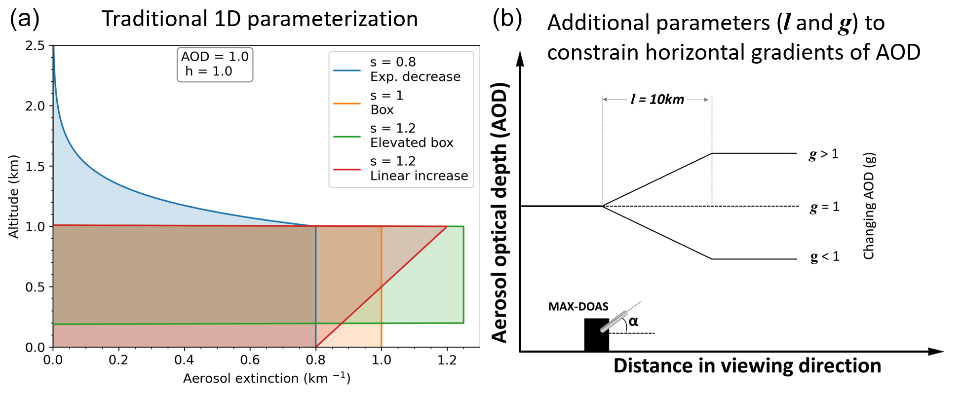
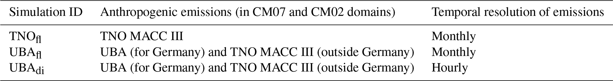
Figure 2(a) Schematic illustration of traditional 1D parameterized profile inversion which constrains AOD, height (h) and shape (s) of the profile. The example shown here corresponds to a scenario with AOD =1.0, h=1.0 and four different profile shapes representing exponential decrease, box profile, elevated box profile and linearly increasing profiles. (b) Additional parameters l and g further constrain the horizontal gradients of AOD for 2D profile inversion. Here, g denotes a linear change in AOD for a distance l along the viewing direction of the MAX-DOAS instrument.
Figure 2 shows the schematic of a traditional profile inversion for an example case of AOD =1.0, h=1 and various parameterizations of s representing the respective profile shapes as well as additional parameters g and l for π-MAX. These additional parameters describe the linear aerosol extinction change (g) from the telescope location to a specific distance (l). Hence, they allow for retrievals of 2D dbAMFs (and aerosol extinction profiles) as a function of distance from the telescope and altitude from the instrument, if measurement in only one azimuth direction is considered. If measurements in several azimuth directions are combined, 3D retrievals can be performed. In the current π-MAX set-up, l is fixed to 10 km. The dSCD measurements in all four directions are used simultaneously with the constraint that the profile at the origin (location of the instrument) is the same for all the telescopes.
The quality of the profile retrieval from π-MAX can be qualified using the rms of the dSCD fit corresponding to each complete elevation sequence. In order to retain only the highest quality profile inversion results, we have retained retrievals corresponding to rms values less than 0.04 times the O4 VCDs.
2.3 In situ chemical and meteorological measurement data
We used the surface temperature, relative humidity and wind measurement data from the Climate Data Center of the German Meteorological Service (Deutscher Wetterdienst) for meteorological evaluation in the CM02 set-up (DWD, 2019). Hourly measurements of surface temperature, relative humidity and wind speed are available for 620, 501 and 283 stations, respectively, in Germany for May 2018; out of these, 178, 197 and 95, respectively, fall within the CM02 domain.
In situ measurements of NO2 and O3 are available from the German Environment Agency (Umweltbundesamt) (Minkos et al., 2019) from 410 and 266 stations, respectively, across Germany for May 2018. Among the 410 NO2 measurement stations, 193 fall within the CM02 domain, out of which 119, 60 and 14 stations represent background, traffic and industrial locations, respectively. For O3, 120 stations are within the CM02 domain, out of which 109, 3 and 8 stations represent the background, traffic and industrial locations, respectively. For most of the stations within the CM02 domain, NO2 is measured online using the chemiluminescence method, in which NO2 is reduced to NO using a heated molybdenum converter prior to its detection (Eickelpasch and Eickelpasch, 2004). Only at Schmücke (DEUB029), a photolytic converter is used in place of the molybdenum converter, whereas at Pfälzerwald-Hortenkopf (DERP017), a CAPS (Cavity Attenuated Phase Shift Spectroscopy) instrument is used for measurement of NO2 (https://www.env-it.de/stationen/public/downloadRequest.do, last access: 13 July 2021). O3 is measured online using the UV absorption technique at all the stations. The measured in situ data are available at 1 h resolution.
3.1 Meteorological evaluation: surface temperature, relative humidity and wind speed
In the online coupled MECO(n) system, COSMO/MESSy instances are not nudged directly towards the reanalysis dataset. Rather, these receive the meteorological boundary conditions from EMAC for the first instance and from the antecedent COSMO/MESSy for each subsequent instance on the four sides of the domain and the damping layer (ca. 11 km for CM50 and CM07 and 10.7 km for the CM02 domain). Hence individual COSMO/MESSy instances of MECO(n) can develop their own dynamics, which might result in a deviation from the actual meteorology. Hofmann et al. (2012) have evaluated the MECO(n) meteorology and demonstrated comparable performance with respect to a similar model with offline coupling. Here, we briefly evaluate the performance of MECO(n) in the CM02 set-up with respect to the measured surface temperature, relative humidity and wind speed close to the surface.
The ability of the model to reproduce the temporal variability at multiple measurement stations can be evaluated using Taylor diagrams (Taylor, 2001), where we show the Pearson correlation coefficient (R), relative root mean square difference (RMSD) and relative standard deviation (RSD) with respect to the hourly resolution measured data. The Taylor diagrams for these parameters are shown in Fig. 3.
Figure 3Taylor diagrams showing the agreement between measured and model-calculated surface temperatures (a) and relative humidity (b) and wind speed (c). Each data point corresponds to an individual measurement station, with a total of 178, 197 and 95 stations for surface temperature, relative humidity, and wind speed, respectively.
For surface temperature, the trends in the hourly-resolved time series agree quite well with Pearson correlation coefficients generally between 0.8 and 0.9. The spatial patterns of the surface temperatures are also represented very well as inferred from small and precise RMSD values of ca. 0.5. RSD values of less than 1 indicate that observed temporal variability in the model has a smaller amplitude than that of the measurements. There is a cold bias of ∼3 ∘C across the domain, which is similar to that observed by Mertens et al. (2016) for Germany in summer. Previous long-term evaluation of the COSMO-CLM model has shown a cold bias of 2–2.5 ∘C compared to observation of the annual mean surface temperature over Germany, which increases in the summertime (Böhm et al., 2006). This bias is most probably due to inaccurate representation of root depth and soil temperature damping in the soil model. For relative humidity, the trends in the hourly-resolved time series agree reasonably well with Pearson correlation coefficient generally between 0.5 and 0.7. Both positive and negative mean biases are observed for the different stations. For wind speeds, the Pearson correlation coefficients are generally between 0.2 and 0.5, but the bias was generally small and in the range of ±1 m s−1.
3.2 Evaluation of surface mixing ratios of NO2
In this section, we present the model results for simulated NO2 surface volume mixing ratios (VMR) and compare with the in situ observations for May 2018. Figure 4 shows the spatial distribution of monthly-mean NO2 VMRs in the lowest vertical layer (0–20 m) for the CM02 domain for the three model set-ups listed in Table 1. The monthly-mean VMRs from the in situ measurement stations are depicted as square, circle and pentagon markers for background, traffic-adjacent and industrial sites, respectively, overlaid on the maps using the same colour scale as that for simulated VMRs.
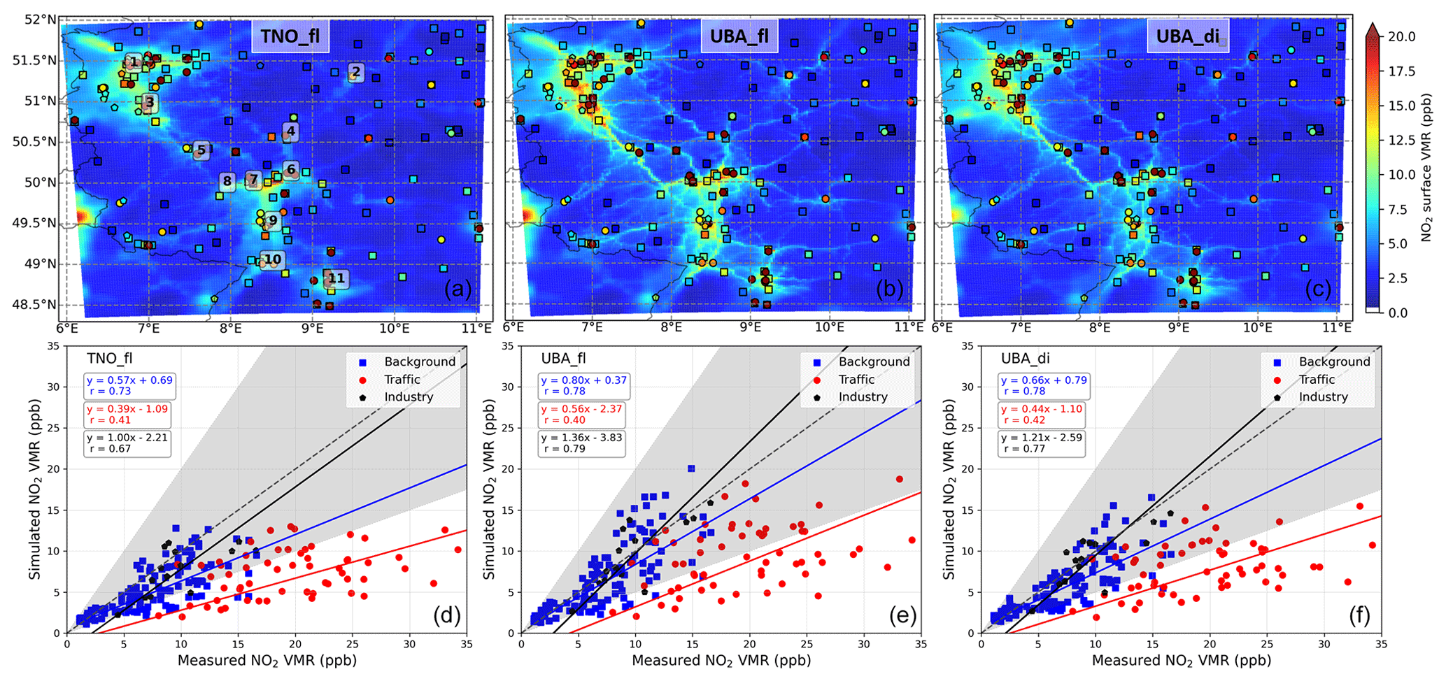
Figure 4(a, b, c) Spatial distribution of monthly-mean NO2 surface VMRs for the three simulations using different emission inventories (a, d: TNO, b, e: UBA without diurnal variations, c, f: UBA with diurnal variations) for CM02 for May 2018. The square, circle and pentagon markers overlaid on the maps represent the monthly-mean measured NO2 VMRs for background, traffic and industrial locations, respectively. The numbers on the top left panel correspond to the following German cities in decreasing order of latitude coordinate values, i.e. 1: Duisburg, 2: Kassel, 3: Köln, 4: Gießen, 5: Koblenz, 6: Frankfurt, 7: Mainz, 8: Bingen, 9: Mannheim, 10: Karlsruhe 11: Stuttgart. (d, e, f) Scatter plot and orthogonal distance regression weighted by the inverse of the square of the standard deviation of simulated monthly-mean NO2 surface VMRs with respect to the in situ measured values for different station types (background: blue square; traffic: red circle, and industrial: black pentagon).
Overall, the spatial distribution of NO2 VMRs is as expected, such that the high values are observed in densely populated areas, e.g. the Ruhr area, Luxembourg, around Frankfurt, Mannheim, Karlsruhe and Stuttgart. For the simulation with the high-resolution UBA emissions, we observe many details in the NO2 surface concentration with higher values coinciding with the major motorways of Germany which were not so obvious with TNOfl (e.g. A61 motorway between Köln and Bingen, A3 between Frankfurt and Bingen, A48 and A1 connecting Koblenz and Luxembourg, and A4 and A9 between Gießen and Leipzig). The performance of the model in reproducing the spatial variability can be quantitatively described using the root mean square deviation (RMSD) between the monthly-mean measured and simulated NO2 VMRs for all the measurement stations combined. We note that using the high-resolution UBA emissions improves the RMSD for background locations from 3.3 ppb (∼45 % of the measured mean) for TNOfl to 2.7 ppb (∼37 %). Since UBA emissions are up to date and are available for the same year as that of simulation, the mean bias for the background locations also improves from −2.0 ppb (−27 %) for TNOfl to −0.5 ppb (−7 %) for UBAfl. At locations near heavy traffic, the bias improved from −12.5 ppb (−63 %) for TNOfl to −10.4 ppb (−52 %) for UBAfl.
Even though the anthropogenic NOx emissions have reduced by ∼15 % over Europe from 2011 (the most recent year for which TNO emissions are available) to 2017 (EEA, 2019), total NOx emissions over Germany are ∼21 % lower in TNO MACC III as compared to UBA. For the TNO MACC III, NOx emissions are lower across all the sectors except for ship transport and comparable for residential and non-industrial combustion. For the three strongest NOx emission sectors, e.g. road transport, energy industries and other industries, TNO MACC III NOx emissions (for 2011) are ∼19 %, 34 % and 18 %, respectively, lower than the UBA NOx emissions (for 2018) (see Fig. A3). Recent top-down emissions estimates over urban centres in Germany have also pointed towards an underestimation of as much as a factor of 2 from the transport sector and 1.5 overall (Kuik et al., 2018) by the TNO MACC III emissions, even by considering a conservative approach. Top-down emission estimates using OMI (Ozone Monitoring Instrument) NO2 measurements also indicated an underestimation of NOx emission by more than 50 % over western Germany and other parts of Europe by the TNO MACC III emission inventory (Visser et al., 2019). It should be noted that exclusion of soil NOx emissions from the TNO MACC III inventory also contributed towards the large underestimation in the estimates by Visser et al. (2019). The underestimation of the a priori NOx emissions is the most important factor for the large negative bias in the TNOfl set-up. Getting up-to-date emission inventories is difficult, and we could only get these data for Germany, but for future studies with simulation involving larger domains, which include more countries, it is recommended to use more up-to-date emission inventories. The situation of underestimation of NOx emissions over Germany (and most parts of Europe) is different from that observed in the USA, where national emissions inventories are biased high by as much as 30 %–60 % (Travis et al., 2016).
Unlike for the background locations, we do not observe a major improvement for the traffic-adjacent locations using the UBA emissions. Even at such high spatial resolution (2.2×2.2 km2), the spatial smoothing leads to insufficient reproduction of peaks for locations close to strong emission sources as also documented by Shaiganfar et al. (2015). Another factor which could contribute to the differences between measured and simulated NO2 is related to the chemiluminescence principle used for measurements: NO2 is first reduced to NO before subsequently reacting with O3 generated within the analyser. This is known to overestimate the actual NO2, because the molybdenum converter within the analyser also reduces the NOx reservoir species (e.g. HNO3, PAN) to NO prior to detection (Dunlea et al., 2007). PAN and HNO3 are more abundant at the traffic and urban locations with a combined monthly-mean mixing ratio of between 0.9 and 1.1 ppb in the UBAdi set-up. This could account for 3 %–10 % of the measured NO2 at the traffic-adjacent locations.
Figure 5 shows a comparison of measured and the simulated NO2 surface VMRs in the CM02 domain as Taylor diagrams for the three different simulations.
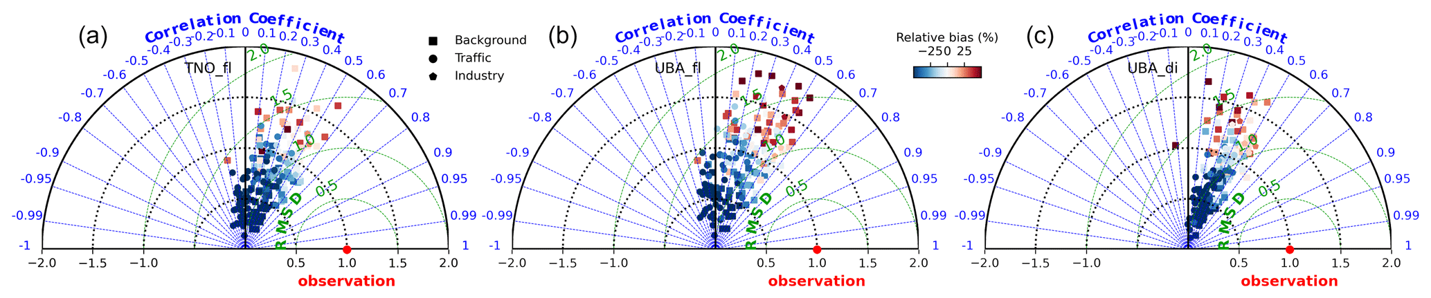
Figure 5Taylor diagrams showing the Pearson correlation coefficients, normalized standard deviation and normalized root mean square difference corresponding to hourly resolution measured and simulated NO2 VMRs (in CM02 domain) for background, traffic and industrial sites represented as square, circle and pentagon markers, respectively. Panels (a), (b) and (c) correspond to the TNOfl, UBAfl and UBAdi set-ups, respectively.
For both TNOfl and UBAfl, we observed rather poor agreement of the hourly temporal variations of the measured VMRs with several stations even showing negative values of R. In Germany, transport emissions account for >45 % of the total NOx emissions, which show a large diurnal variability (greater than 200 % peak to peak; see Fig. A1). These variabilities are generally not taken into account for regional model simulations and have shown to cause larger bias during peak traffic hours on weekdays (Kuik et al., 2018). In the UBAdi set-up, accounting for diurnal and day-of-the-week variability in the anthropogenic emissions shows significant improvement with R values of between 0.3 and 0.6, smaller RMSD values and more consistent agreement for different stations. However, we also note that overall negative bias is increased for the UBAdi set-up compared to UBAfl. The diurnal profiles of emissions in the transport sector increase the NOx amount to more than twice as much during the daytime when the atmospheric lifetime is lower and decreases to less than one-quarter during the night when lifetime is high. Hence, overall, the monthly-mean surface NO2 VMR decreases when a diurnal profile is applied to NOx emissions. The normalized standard deviation (relative to the standard deviation of measured VMRs) improves by inclusion of diurnal profiles, as we observe more stations with values in the 0.5–1.5 range.
Using the different COSMO/MESSy instances of the MECO(3) system, we are able to investigate the importance of model resolution if the same emission inventory is used for different model resolutions. Figure C2 shows the spatial distribution of simulated NO2 surface VMRs and the agreement with measurements for the CM07 set-up in a similar way as Fig. 4 for CM02. We note that for TNOfl there is only very little further detail in the spatial distribution for CM02 as compared to CM07. Meteorology (e.g. wind patterns) might be better resolved using a fine model resolution on individual days. Still, when averaged over several days, these will be smoothed, and the spatial patterns would be limited by the resolution of the input emissions inventory. Consequently, we also did not observe any significant improvement in the RMSD (45 %) between the monthly-mean measured and simulated NO2 VMRs as compared to the CM07 simulation (RMSD =48 %) using the TNO MACC III emission inventory. In contrast to this, using the high-resolution UBA emissions, the spatial details as depicted in CM02 smear out in the CM07 instance. For both UBAfl and UBAdi set-ups, the RMSD improves from ∼45 % for the CM07 to ∼37 % for CM02, showing the added value of the higher resolution simulation. Hence, for studies where small scale variability is crucial, it is important to use a high-resolution model together with an input emission inventory of similar resolution.
Further reasons which could account for the lower bias of the NO2 VMR in the model could be related to stronger advection and vertical mixing. The vertical distribution of NO2 is evaluated in Sect. 3.3.2. Regarding advection, the wind speeds at 10 m altitude in the CM02 domain have been compared with measurements at 95 stations located within the CM02 domain (see Sect. 3.1). A small positive bias of ca. 0.5 m s−1 was found. A cold bias of ∼3 ∘C (a general feature of COSMO in summer over western Europe; Böhm et al., 2006) was observed across the CM02 domain, but that should not cause a lower bias in the simulated NO2 VMRs.
An evaluation of surface O3 VMRs with respect to the in situ measurements in a similar way as that for NO2 is discussed in Appendix B.
3.3 Comparison of tropospheric columns
3.3.1 Vertical column densities
The general approach involving an evaluation of model VCDs involves summing up simulated NO2 partial columns (concentration times height of individual model grid boxes) vertically. The same approach can be applied both for evaluation of VCDs with respect to satellite and MAX-DOAS observations. However, different inferences can be drawn from these comparisons owing to the difference in sensitivity volumes. When compared to satellite observations, a larger weight is assigned to NO2 at higher altitudes where satellite sensitivity is higher. Mertens et al. (2016) evaluated the NO2 VCDs from the MECO(2) system using SCIAMACHY observations and found that the model performed well in reproducing the spatial variability. In contrast to the satellite observations, MAX-DOAS measurements have higher sensitivity within the boundary layer. From the CM02 domain of all three set-ups, we learn that the partial column in the lowest 1 km accounts for ∼80 % of the tropospheric NO2 column.
However, a generalized vertical integration on a regular model grid can introduce artefacts, because MAX-DOAS measurements are rather sensitive to air mass in the viewing direction for distances of up to a few kilometres. The artefacts increase with increasing spatial heterogeneity. In order to consider NO2 only in the viewing direction of the four telescopes, we first linearly interpolated the simulated concentrations along the respective viewing directions of the telescopes (see e.g. Fig. 1). The tropospheric VCDs are calculated in the following two steps: (1) summing up the partial VCDs vertically up to a height of 4 km and (2) taking the mean of VCDs up to a fixed distance (3 km as a first estimate) only in the line of sight of the telescope. An example time series of the simulated VCDs for the UBAdi set-up is shown in Fig. 6 along with the measured MAX-DOAS VCDs.
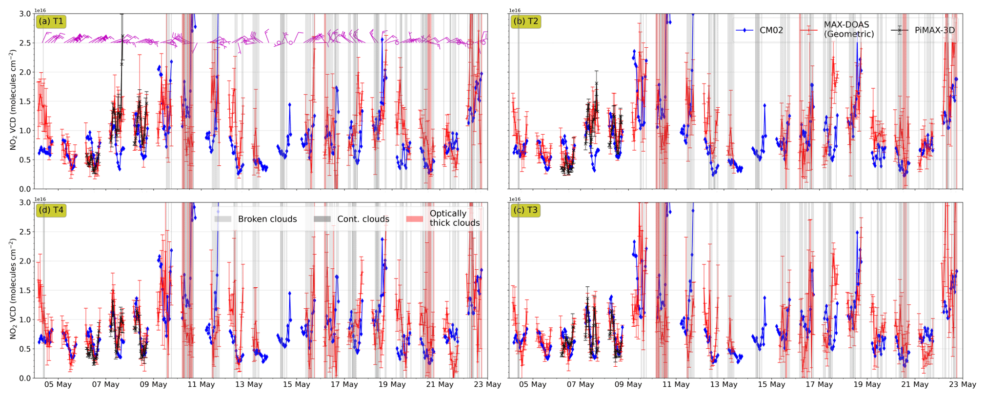
Figure 6Comparison of NO2 VCDs along the viewing directions of the four telescopes (T1–T4) simulated using the UBAdi set-up in the CM02 domain. MAX-DOAS VCDs are retrieved using geometric approximation (red markers) for the complete measurement period and using π-MAX for 3 d (black markers). The error bars represent the hourly 1σ standard deviations. The shaded regions in the time series represent various categories of clouds as described in the legend. The purple barbs in panel (a) show the measured wind speed and wind directions, with half arrows, full arrows and flags corresponding to wind speeds of 1, 2 and 5 m s−1, respectively.
Figure 7 shows the agreement between the MAX-DOAS geometric VCDs and the simulated VCDs as scatter plots for the three different set-ups in different panels. The frequency distributions of the measured and the simulated VCDs are also shown next to the corresponding panels.
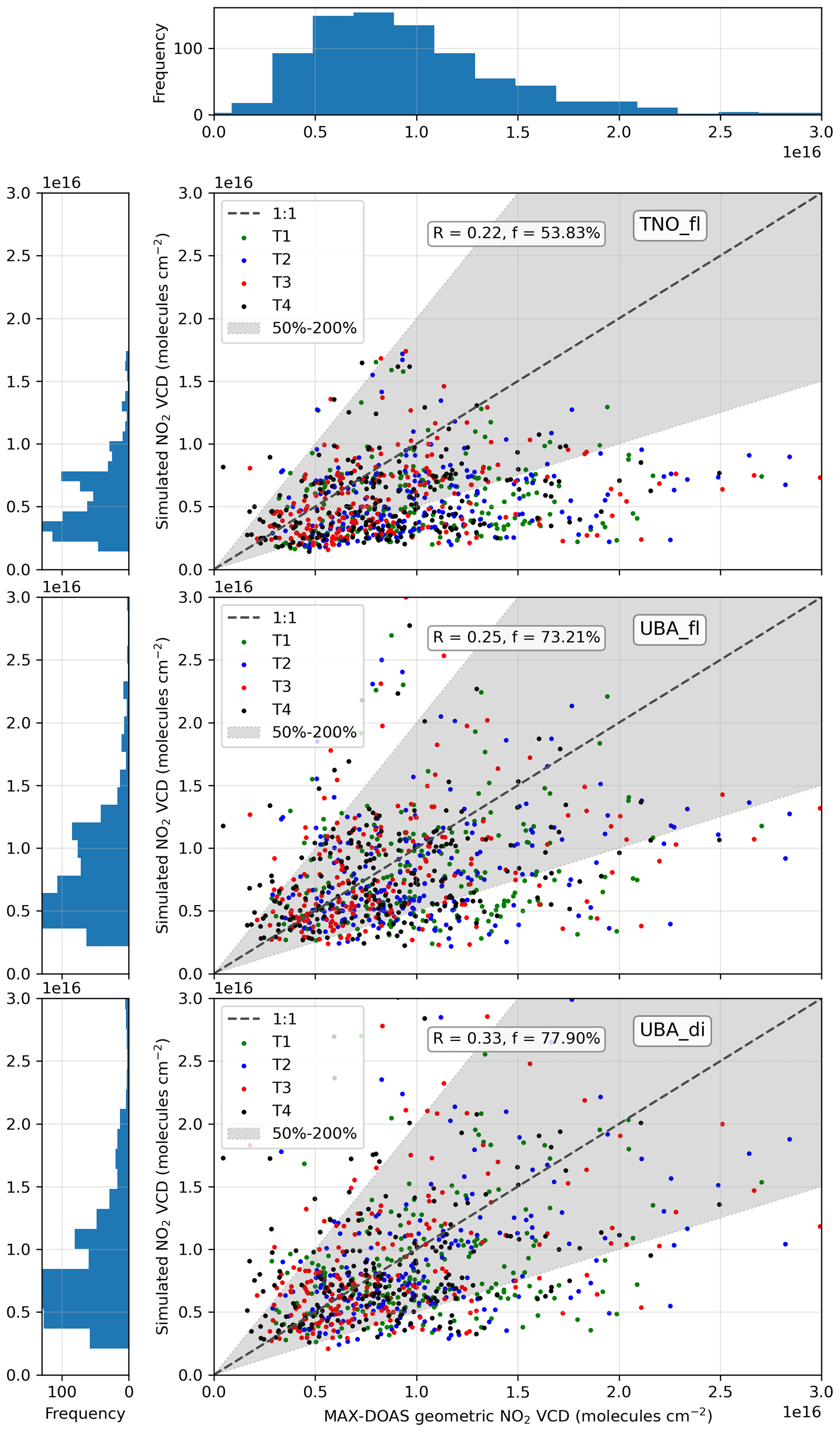
Figure 7Scatter plot of simulated VCDs against measured VCDs for all four telescopes combined for 30∘ elevation angle. Individual points correspond to the hourly-mean VCD values. The top, middle and bottom panels correspond to TNOfl, UBAfl and UBAdi, respectively. R represents the Pearson correlation coefficient, and f represents the fraction of simulated NO2 VCDs no less than half and no greater than twice the magnitude of geometric VCDs. The frequency distribution of the measured VCDs is shown above the first panel, and those for the simulated VCDs from the three set-ups are shown on the left of the respective scatter plots.
We observe a large scatter between the MAX-DOAS and simulated VCDs in all three model set-ups, but the best agreement was observed for the UBAdi set-up with 78 % of the simulated VCDs no less than half and no greater than twice the magnitude of the measured VCDs and the best Pearson correlation coefficients (R=0.33) among the three. For TNOfl, large underestimation of VCDs was observed, as also seen for surface VMRs in Sect. 3.2. The markedly lower bias (see Tables C2 and C3) can be attributed to significantly lower input NOx emissions (e.g. ∼40 % lower compared to UBA emissions over Germany for 2018). Using UBA emissions reduces the bias from 37 %–47 % to 9 %–21 % for the different telescopes. Adding diurnal variability to emissions reduces the bias further (−1 %–13 %), as it increases the emissions during the daytime (see Fig. A1 and Table C2). While the model was able to capture the general trend in day-to-day variability, the intra-day variability could not be reproduced on most of the days. The agreement was much better on the days with clear-sky conditions (4–9 May) and periods of other days with cloud-free conditions. From Tables C2 and C3, we note that the R and RMSD values improve from 0.27–0.39 and 57 %–67 %, respectively, in the UBAdi set-up for all measurements of all four telescopes to 0.37–0.52 and 50 %–53 % if the analysis is restricted to cloud-free conditions. Between 5 and 9 May, the simulated VCDs matched almost exactly to the MAX-DOAS VCDs for the telescopes T3 and T4, but for T1 and T2 the agreement was not as good. Several factors can contribute to the observed differences, but there are at least two shortcomings related to VCD comparison, which hinder a conclusive assessment.
-
The MAX-DOAS VCDs are calculated using the geometric approximation which assumes a single scattering event of the incoming photons above the trace gas layer. This yields reasonable VCDs for clear-sky conditions with a low aerosol load scenario (Shaiganfar et al., 2011; Kumar et al., 2020). More accurate VCDs can be retrieved using the profile inversion approach, which also accounts for aerosol extinction profiles and the relative sun geometry. For the three clear-sky days with low aerosol load, we also performed trace gas profile inversion using the sophisticated π-MAX approach, which also considers a linear change in NO2 concentration along the line of sight. The VCDs retrieved using π-MAX (shown in Fig. 6) agree quite well with the geometric VCDs for these days. For most of the profile inversion algorithms used currently (Frieß et al., 2019, and references therein), it is assumed that trace gases are homogeneously distributed and that MAX-DOAS is equally sensitive within the horizontal sensitivity distance; this can be an additional source of error. Previous studies (e.g. Blechschmidt et al., 2020, and Vlemmix et al., 2015) used the optimal estimation-based profile inversion approach, which also requires an a priori estimate of the NO2 vertical profile and can bias the model evaluation if the assumed a priori profile is similar to that simulated by the model. The averaging kernels (Ak) can be applied on the model partial column (Vk) to calculate the modified VCD (VCDcorr), using the a priori profile according to Eq. (3), which can be directly compared to the MAX-DOAS VCDs.
For high Ak (i.e. close to 1 ), is limited by the simulated Vk, whereas for low Ak (i.e. close to 0; where MAX-DOAS sensitivity is limited), is limited by the a priori profile. Hence, the choice of the a priori profiles can impact the comparison in the latter scenario.
-
While calculating the simulated VCDs, model NO2 fields are given equal weights up to a distance of 3 km in the viewing direction and 4 km altitude. As mentioned previously, distances in both dimensions were only a first estimate, and the actual MAX-DOAS sensitivity distances in both dimensions might vary according to the aerosol load, trace gas distribution, viewing geometry with respect to the sun and presence of clouds. Moreover, even within the actual sensitivity volume, the sensitivity might vary as a function of distance from the telescope. Blechschmidt et al. (2020) have previously demonstrated that accounting for vertical sensitivity of MAX-DOAS (via averaging kernels) does not noticeably affect the simulated VCDs, because most of the NO2 is located within the boundary layer, and the averaging kernel profile has a similar shape as the model NO2 vertical profiles. Hence, vertical sensitivity was not an issue where most of the NO2 is located. However, if the profile is elevated, then this may no longer hold true. Nevertheless, sensitivity in the horizontal direction still needs to be accounted for, as large heterogeneity is expected close to the emission sources for short-lived species like NO2. The studies by Blechschmidt et al. (2020) and Vlemmix et al. (2015) proposed the relatively coarser model resolution of up to 7×7 km2 as one possible reason for this discrepancy. For comparison with ground-based measurements (e.g. MAX-DOAS), it is crucial to have model simulations with a grid resolution finer than or the same as the typical sensitivity ranges of the measurements. If that is not the case, spatial heterogeneity within the model grid box would result in underestimation of the enhancement and overestimation of the background values due to spatial smoothing. For MAX-DOAS measurements at 30∘ elevation angle, the horizontal sensitivity distance (HSD) can be approximated using the boundary layer height (BLH) (), which would be in the range of 1–3 km in the daytime. However, the exact HSD also depends on the aerosol conditions, which can vary significantly over time and should be retrieved from measurements.
In the next section, we will address these shortcomings by calculating the differential slant column densities (dSCDs) using the simulated NO2. Simulated dSCDs can be directly compared to the corresponding quantities derived from the DOAS analyses while also avoiding several assumptions and approximations discussed earlier. The dbAMFs used for dSCD calculation inherently account for the aerosol conditions and hence also address issues related to spatial sensitivity (see Sect. 2.2.2). This also provides a way for quantification of the horizontal sensitivity distances of MAX-DOAS measurements.
3.3.2 Slant column densities
Calculation of simulated dSCDs
For calculation of dSCDs from the model simulated NO2 fields, we mimic the viewing geometry and sensitivity volume corresponding to MAX-DOAS measurements using the differential box air mass factors as described in Sect. 2.2.2. Using MAX-DOAS, we probe the vertical and horizontal variation of NO2 concentrations by measuring at various elevation angles. The sensitivity of the MAX-DOAS measurements at a given elevation angle (EA) is described by the differential box air mass factors (dbAMFs). An example of the dbAMFs along the viewing direction of telescope T1 for 9 May 2018 14:00 UTC for EAs ranging from 3 to 30∘ is shown in Fig. 8. In each viewing azimuth (corresponding to T1–T4) and for each EA (α; between 2 and 30∘) we perform a 2D summation of partial VCDs (Vi,k) weighted by the differential box air mass factors () (unitless), along the distance from MAX-DOAS (indexed as i) and altitude above the instrument (indexed as k):
with
where ci,k and dhi,k represent the concentration (molecules cm−3) of trace gas in the grid with a thickness of dhi,k (cm).
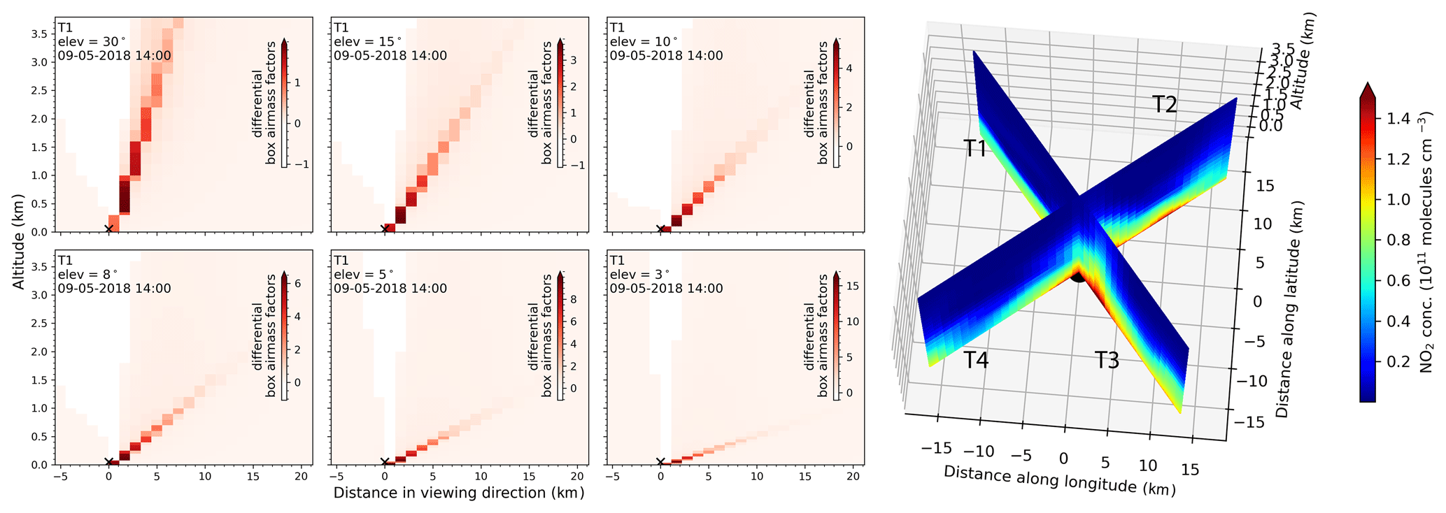
Figure 8Left: the differential box air mass factors (dbAMFs) for 30, 15, 10, 8, 5 and 3∘ elevation angles retrieved using 3D profile inversion of measured O4 dSCDs along the direction of telescope T1. Please note the different colour scales of differential dbAMFs used for the different elevation angles. Right: simulated NO2 concentrations from the UBAdi set-up in the CM02 domain from surface up to an altitude of 2.5 km along the viewing directions of the four telescopes T1, T2, T3 and T4 on 9 May 2018 14:00 UTC.
Using Eq. (4), we can estimate the EA dependent horizontal sensitivity distances (HSD) in the viewing direction of the MAX-DOAS as the distance from the instrument which accounts for 90 % of the simulated dSCDs. Figure C3 shows the HSD for all the off-axis elevation angles for the four telescopes. The mean HSD increases from 3–4 km for 30∘ EA to 8–9 km for 3∘ EA. In contrast to the comparison of the geometric VCDs in the previous section, which is limited to only one EA, we can evaluate the dSCDs at various EAs with varying sensitivity volume from the location of the instrument. Additionally, while calculating the dSCDs, we also account for the horizontal heterogeneity and varying sensitivity within the sensitivity volume in the viewing direction.
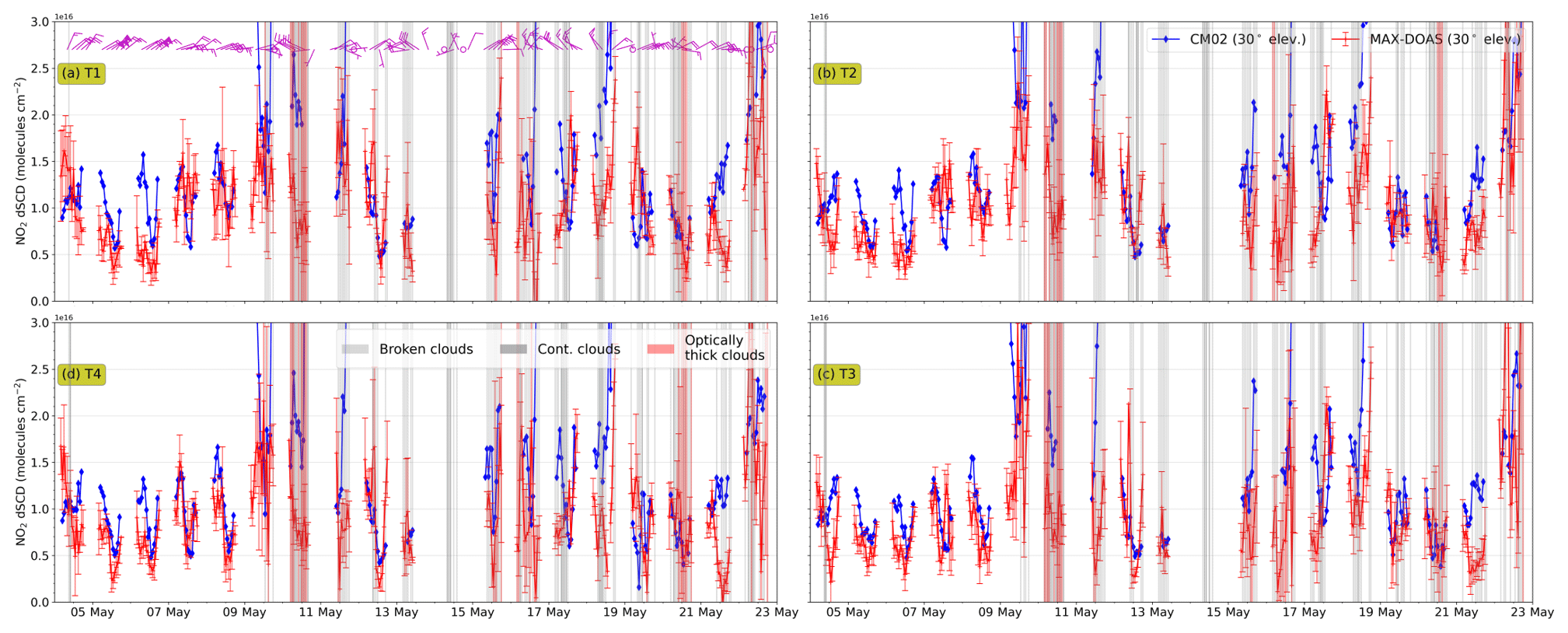
Figure 9Comparison of NO2 differential slant column densities at 30∘ elevation angle of the four telescopes simulated using UBAdi in the CM02 domain. The shaded regions in the time series represent various categories of sky conditions as described in the legend.
Figure 9 shows an example time series of measured and simulated dSCDs for UBAdi for 30∘ EA. Comparing these values to the VCDs shown in Fig. 6, we observe that the simulated dSCDs are higher than the calculated VCDs as shown in the previous section, implying dAMFs at 30∘ EA are larger than 1. This is also observed under the cloud-free conditions, which corroborates the drawback in the geometric approximation and assumption of spatial homogeneity in the viewing direction.
Evaluation of simulated dSCDs
Figure 10 shows the distribution of measured and simulated dSCDs (different colours for the different model set-ups described in Table 1) for the various elevation angles as box and whiskers plots for the four telescopes in separate panels. Measurements performed at low EAs have large light paths and are more sensitive to air mass close to the surface (higher dbAMFs; see Fig. 8); hence, larger dSCDs are observed for the low EAs. Surprisingly, we did not observe major differences in the measured as well as simulated dSCDs among the four telescopes, besides slightly higher values for T2, which points towards the city centre of Mainz and lower values for T4, which spans mostly agricultural lands for a distance of 10 km. This can partially be explained by the prevailing wind directions (Fig. 6a), as for most of the time easterly winds bring the air mass from the urban locations to the agricultural lands.
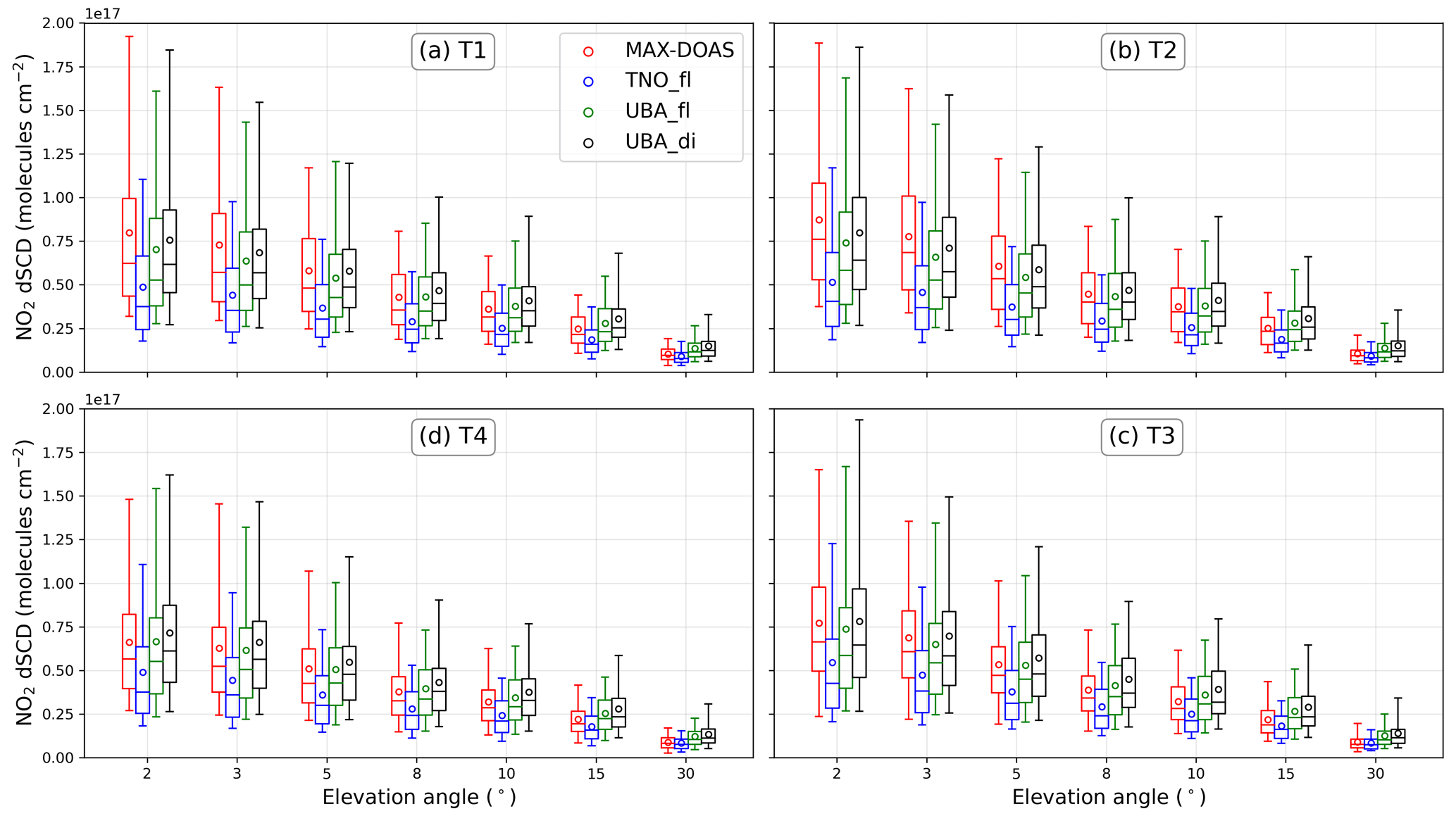
Figure 10Box and whiskers plots for the different telescopes (a–d) showing the distribution of measured and simulated dSCDs for the three different model set-ups (depicted in different colours) for various elevation angles (2, 3, 5, 8, 10, 15, and 30∘).

Figures 9 and 11 show example time series of measured and simulated dSCDs (for UBAdi) for 30 and 3∘ EAs, respectively. Various statistical parameters corresponding to the agreement between MAX-DOAS and model simulation for individual telescopes and EAs are summarized in Table C2 for all measurements and in Table C3 for cloud-free cases only. For 30∘ EA, we did not observe any significant change in the agreement of temporal variability (i.e. R) between model and MAX-DOAS, whether we compare dSCDs or VCDs. However, significantly more information is gleaned with respect to the available dSCDs corresponding to all the off-axis EAs at which measurements were performed. Instead of comparing only one VCD value for a complete elevation sequence, we include dSCDs corresponding to each of the elevation angles. For example, in Fig. 11, we observe a much better agreement between the measured and simulated dSCDs at 3∘ EA, especially on the cloud-free days.
In Fig. 12, we show the comparison of measured and simulated dSCDs for the three different model set-ups in different panels for all the EAs and all the telescopes. The frequency distribution of the measured dSCDs at various EAs are shown above the top panel, while those for the simulated dSCDs are shown in the panels left of the scatter plot of the corresponding model set-ups.
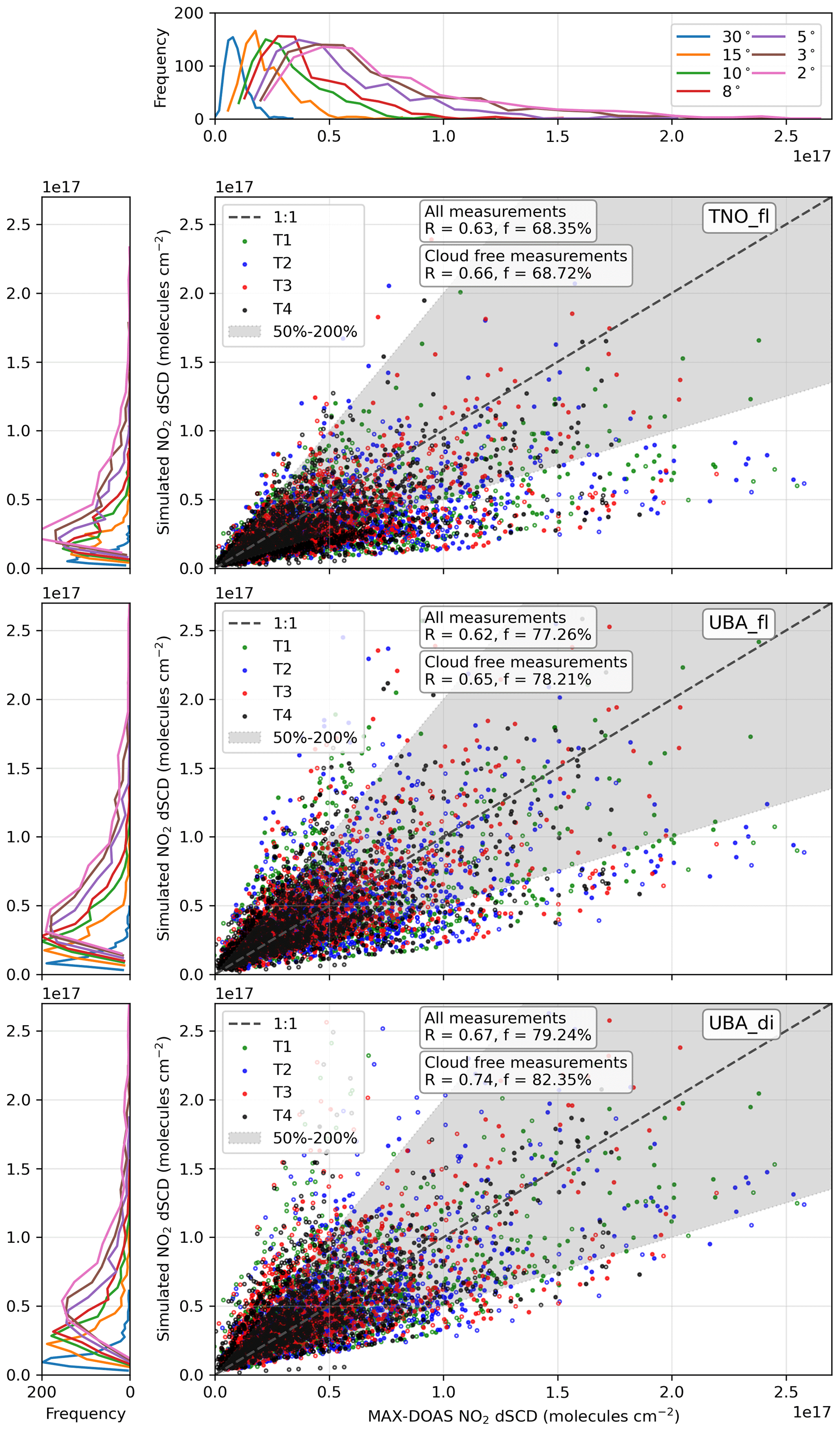
Figure 12Scatter plot of simulated dSCDs against measured dSCDs for all the four telescopes combined for the elevation angles 2, 3, 5, 8, 10, 15 and 30∘. The filled circles correspond to the cloud-free scenarios, while the empty circles correspond to the cloudy conditions. The Pearson correlation coefficient (R) and the fraction of simulated dSCDs within 50 %–200 % of the measurements (f) are annotated in the respective panels separately for all measurements and for cloud-free conditions only. The top, middle and bottom panels correspond to TNOfl, UBAfl and UBAdi, respectively. The frequency distribution of the measured dSCDs is shown above the first panel, and those for the simulated dSCDs from the three set-ups are shown on the left of the respective scatter plots.
We observe a good correlation between the measured and simulated dSCDs (R=0.63, 0.62 and 0.67 for TNOfl, UBAfl and UBAdi, respectively), which further improves (R=0.66, 0.65 and 0.74) if the comparison is restricted to cloud-free cases only. Similar to the VMR and VCD comparisons, the best accountability was observed for UBAdi, with ∼82 % for the simulated dSCDs no less than half and no greater than twice the magnitude of the measurements for cloud-free cases. The frequency distribution of the measured dSCDs follows a right-skewed normal distribution for all the EAs, which is also represented best by the UBAdi set-up. The width of the peak of the frequency distribution broadens from high to low EAs, representing a larger scatter in the measurements at low EAs. For UBAfl, the extreme values (less than half or more than double of measurements) were mostly observed for cloudy sky conditions. Since clouds are not considered in the radiative transfer simulations and therefore also not in dAMF retrieval, these only affect the measured dSCDs. The improved agreement between simulated and measured dSCDs for the cloud-free conditions are more obvious for the individual EAs (see Tables C2 and C3) with significantly higher Pearson correlation coefficients and smaller RMSD values.
From Tables C2 and C3, it can be inferred that the agreement between measured and simulated dSCDs improves at lower EAs, which also indicates a better performance of the model in the layers close to the surface. For example, for both the UBAfl and UBAdi set-ups, a large positive bias in the range 27 %–42 % was observed at 30∘ EA, but for low EAs (e.g. ≤8∘) small biases in the range of +7 % and −15 % were observed for all the azimuth directions in the cloud-free cases. However, more pronounced negative biases were observed for TNOfl simulation even at low elevation angles. A positive bias at 30∘ EA is most likely due to the stronger vertical mixing in COSMO/MESSY as also indicated by Mertens et al. (2016). Due to the stronger mixing, a large fraction of NO2 reaches higher altitudes in the model, which has a strong weight for the dSCD calculation at high EAs.
Previous studies in which models were compared with MAX-DOAS indicated that the major disagreements arise due to weekday and weekend differences and inappropriate representation of the diurnal cycle of emissions (Blechschmidt et al., 2020; Vlemmix et al., 2015). We use the measurements at a low elevation angle (e.g. 3∘) to investigate if the model can reproduce the measured diurnal profiles and weekday–weekend differences of NO2 dSCDs. A low elevation angle was chosen, because the corresponding measurements have higher sensitivity close to the ground where a major fraction of NOx is emitted from sectors which show strong diurnal variability.
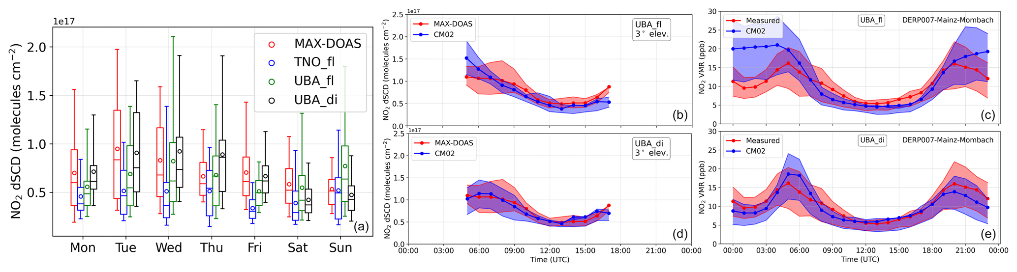
Figure 13(a) Box and whiskers plot showing the distribution of NO2 dSCDs at 3∘ elevation angles for MAX-DOAS and the three different model set-ups for different days of the week. Mean hourly diurnal profiles of measured and simulated NO2 dSCDs at 3∘ elevation angle for T1 for the UBAfl (b) and UBAdi (d) set-ups. The shaded region above and below the mean line denote the 75th and 25th percentiles, respectively. Diurnal profiles of measured and simulated NO2 surface VMRs measured at a background site (Mombach, ∼ 3.5 km north of MPIC) for the UBAfl (c) and UBAdi (e) simulations.
The left panel in Fig. 13 shows the distribution of measured and simulated NO2 dSCDs at 3∘ EA, for all telescopes combined, binned according to the day of the week. The diurnal profiles of the measured and simulated dSCDs are shown in the middle panel of Fig. 13 for UBAfl in the top panel and for UBAdi in the bottom panel. A similar plot for NO2 surface VMR at the background site Mombach (∼3.5 km north of MPIC) is shown in the right panel. The lowest measured dSCDs are observed on the weekends. However, such a distinct weekday–weekend difference was not observed for TNOfl and UBAfl simulations, supporting the fact that the observed differences were primarily because of change in emissions and not due to varying meteorological conditions. Smaller weekend dSCDs were only for the UBAdi set-up, which also accounts for weekday and weekend differences in NOx emission from the transport and residential combustion sectors. Concerning the diurnal variation, both UBAfl and UBAdi show smaller NO2 dSCDs and surface VMRs during the daytime, which agrees reasonably well with the measurements in both set-ups. However, stronger discrepancies are observed during early morning and late evening for UBAfl. The discrepancy is even larger for the UBAfl surface concentration at night-time (Fig. 13). While emissions primarily drive the surface VMRs during night-time, dilution in the higher boundary layer and chemical loss due to OH in the daytime counters the stronger emissions. We further investigated the diurnal patterns of VCDs and surface VMRs (Fig. C4) in the UBAfl set-up and found that the magnitude of diurnal modulation in the hourly mean was ∼350 % peak to peak, while the same was only ∼80 % for VCDs. This difference in the magnitude of diurnal variability indicates a stronger role of the boundary layer height evolution as compared to the chemical loss due to short lifetime towards offsetting the effect of higher NOx emissions during the daytime. From Fig. 13, it is evident that the use of diurnally varying emissions is necessary to reproduce the observed diurnal variability of NO2. For the complete time series of dSCDs, we also observe much improved Pearson correlation coefficients in the range of 0.5 and 0.8 if diurnal and day-of-the-week variability in emissions are considered in UBA emissions as compared to those simulated using “flat” emission profiles (see Table C3). For model studies concerning satellite measurement having afternoon overpasses (e.g. OMI, TROPOMI), consideration of these factors for the anthropogenic emissions will have a relatively weak effect in our study domain or similar urban environments. For the biomass burning regions (e.g. tropical forests, southern Africa), strong NOx emissions are typically observed during midday, which results in a diurnal profile of NO2 columns with a broad daytime peak (Boersma et al., 2008). Consideration of diurnal profiles of emissions in model simulations is crucial for comparisons with satellite observations in these regions (Miyazaki et al., 2012; Boersma et al., 2008).
We performed high spatial resolution (up to 2.2×2.2 km2) regional model simulations focussed on south-west Germany to evaluate the short-lived pollutant NO2 using MAX-DOAS and a network of in situ measurements. Three different MECO(3) simulations were performed in order to investigate the importance of model spatial resolution and the influence of spatial and temporal resolution of input emission inventories. Anthropogenic emission inventories generally used for model simulations (e.g. TNO MACC for Europe) do not cover the most recent periods in most of the cases and are available at spatial resolutions coarser than that of the model. We show that the spatial patterns of NO2 are best reproduced in the UBAfl set-up, in which an up-to-date and high-resolution (1×1 km2) input emission inventory (UBA) is used. In the UBAdi set-up, use of accurate temporal profiles (e.g. diurnal and day of the week) of the road transport and residential and non-industrial combustion emissions improves the agreement of the temporal profiles at individual measurement stations. An improved agreement was observed at the background and industrial locations with an overall bias of less than 10 % for the UBAdi set-up. However, the model largely underestimates the NO2 VMRs (by up to 50 %) at the traffic-adjacent locations. For the background locations, the mean diurnal profiles were accurately simulated in the UBAdi set-up. Biases were stronger if the fine-resolution emissions were used for a coarser resolution model simulation (e.g. 7×7 km2). In contrast, a finer-resolution model employing a coarse emission inventory did not result in the addition of large spatial details.
We employed the measurements of a four-azimuth MAX-DOAS instrument from Mainz to first compare the tropospheric NO2 VCDs. The day-to-day variability was reasonably well reproduced by the model in the UBAdi set-up for all four viewing directions with biases of between −10 % and 2 %. To further augment the surface VMR and tropospheric VCD evaluation, we apply a consistent approach of comparison of the so-called differential slant column densities (dSCDs), which, we suggest, comes with several advantages. Firstly, dSCDs are available for a number of elevation angles, each of which has distinct sensitivities to the different vertical level of the troposphere. Hence, this approach enables an evaluation of the vertical distribution of NO2 in the model. Additionally, the horizontal sensitivity distance of the MAX-DOAS instrument also changes for different elevation angles, as described by the corresponding differential box air mass factors. Hence, when using the measurement at one single location, model evaluation can be performed for various sensitivity volumes. Secondly, as compared to the VCD comparison, which gives one comparable quantity per complete elevation sequence of MAX-DOAS measurements, dSCDs provide a way to evaluate the simulation against the measured values for each elevation angle. Finally, for the dSCD comparison, we succeed in overcoming the uncertainties introduced by the assumption of a homogeneous spatial distribution of NO2 and in some cases a priori estimates of its vertical distribution for the retrieval of VCDs from the MAX-DOAS measurements.
We evaluated the simulated dSCDs in the four azimuth direction for seven elevation angles (EA) ranging from 2 to 30∘. We observe a similar variation of measured and simulated dSCDs for various EAs, indicating a reasonable vertical distribution of NO2. The agreement between model and simulation improved for lower elevation angles, indicating better accountability at near-surface layers. The agreement further improved if only the measurements in cloud-free conditions were considered for the comparison. We did not observe large differences in the measured dSCDs in the four azimuth direction because of the prevailing wind direction from urban areas. We also show that the consideration of diurnal profiles of the anthropogenic emissions is crucial for comparison with NO2 dSCDs and VMR measurements for early morning and night-time hours. For the afternoon hours, however, even up to 50 % higher anthropogenic NOx emissions only have a minor effect on ambient VMRs and dSCDs due to enhanced dilution in the high daytime planetary boundary layer and its short atmospheric lifetime.
Over the last 2 decades, several MAX-DOAS measurements have been reported from locations across the world, which have substantially contributed to the evaluation of satellite observations. We think that the complexity and uncertainties involved in VCD retrieval from the MAX-DOAS measurements have so far hindered a similar scale application in model evaluation. The consistent dSCD comparison approach proposed in our study validates such usage of these valuable datasets, which can be used to evaluate the vertical distribution of trace gases within the boundary layer.
Both TNO MACC III and UBA emissions are available at a temporal resolution of 1 year. The monthly profiles of the anthropogenic emissions depend on the emitted species, emissions sectors and the country. For Europe, these factors are also provided by Builtjes et al. (2002) and are used to create monthly resolution emissions. Builtjes et al. (2002) and Schaap et al. (2005) also provide recommendations for sector-specific fine temporal profiles (day of the week and diurnal) of emissions (see Fig. A1). The fine temporal profiles are applied only in the UBAdi set-up using the MESSy ONEMIS submodel as described in Sect. 2.1. The recommendation of Builtjes et al. (2002) and Schaap et al. (2005), however, do not differentiate between the diurnal profiles of emission between weekdays and weekends, which is crucial for the road transport emissions. Hence, for the road transport sector, we used the actual hourly vehicle count on the A60 motorway for 2018, and we derived the temporal emission profiles assuming a direct scaling between the number of vehicles and emissions. The actual vehicle counts are provided by the automatic vehicle counter and are available at https://www.bast.de/BASt_2017/DE/Statistik/statistik-node.html (last access: 13 July 2021). From Fig. A1, we note that for weekdays the derived profiles look similar to those recommended by Schaap et al. (2005). However, for the weekend, the shape of the diurnal profiles are markedly different from the factors derived using actual vehicle counts, which show a single broad afternoon peak.
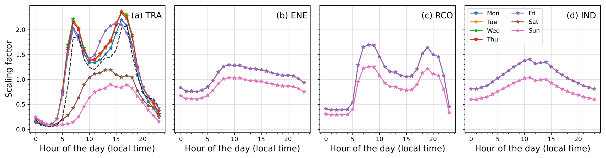
Figure A1Temporal profiles of NOx emissions from various sectors. “TRA”: road transport, “ENE”: energy generation, “RCO”: residential and non-industrial combustion, “IND”: industries. For TRA, lines and markers correspond to the profiles derived using actual vehicle count, while for others profiles are derived according to the recommendation of Schaap et al. (2005). For TRA, the recommendations of Schaap et al. (2005) are shown as the dashed line in panel (a).
Please note that the current implementation of incorporation of diurnal emission factors is limited to surface emissions. Since for “ENE” and “IND” sectors, a significant fraction is emitted at high altitudes, the day of the week and diurnal profiles could not be applied to these sectors. However, from Fig. A1, we note that these temporal variations are not as strong as for “TRA” (>200 % peak to peak) and “RCO” (>120 % peak to peak) sectors. Moreover, for Germany, ENE and IND account for only ca. 14 % and ca. 18 % of the total NOx emissions as compared to ca. 45 % from TRA only. Hence, we only expect a minor effect of including the day of the week and hourly temporal factors of emissions of ENE and IND sectors on the total NOx emissions.
Figure A3 shows the contribution of different sectors to the total NOx emissions in the TNO MACC III (for 2011) and UBA inventory (2018) for Germany. The individual sectors are agriculture (AGR); energy industries (ENE); other industries (IND); residential and non-industrial combustion (RCO); fossil fuel production and distribution (REF); water navigation (SHP); solvent and other product use (SOL); road transport (TRA); and waste collection, treatment, and disposal activities (WST). The major under-representations of the TNO MACC III emissions are the sectors road transport, energy industries and other industries, while ship emissions are higher in TNO MACC III. It should also be noted that agricultural emissions are not included in TNO MACC III inventory (Kuenen et al., 2014), while these are included in UBA inventory. Here we would like to point out that in our simulations using UBA emissions, emissions due to use of organic and inorganic fertilizers are doubly counted within Germany, as these are also calculated online using the ONEMIS submodel. We have checked the contribution of these two sources in the total NOx emissions within Germany and these are 8 % of the total. However, this is within the uncertainty of the NOx emissions in the inventories which are in the order of 20 % (Solazzo et al., 2021).
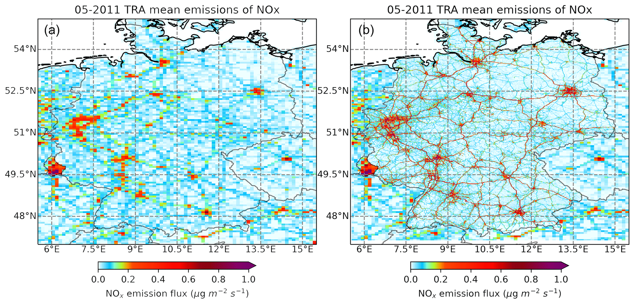
Figure A2NOx emission flux from the road transport sector for (a) TNO MACC III emissions for May 2011 (Kuenen et al., 2014) and (b) composite UBA with Germany (May 2018) and TNO MACC III emissions outside Germany (May 2011).
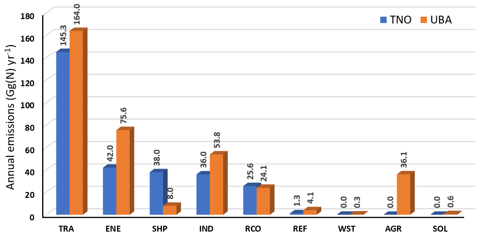
Figure A3Contribution of individual sectors towards the total NOx emissions within Germany for the TNO MACC III emission inventory for 2011 (blue) and UBA emission inventory for 2018 (orange).
Figure B1 shows the spatial distribution of the monthly-mean O3 VMRs and agreement with respect to the measured values in a similar way as for NO2 in Fig. 4. We observe a rather smooth spatial distribution of O3 as compared to that of NO2, with high values relatively far from the NO2 hotspots. We observe an overestimation for smaller O3 VMRs for all three model set-ups. Since ozone is formed photochemically in the troposphere, we have further investigated the agreement separately for daytime (07:00–18:00 UTC) and night-time for the UBAdi set-up in Fig. B2.
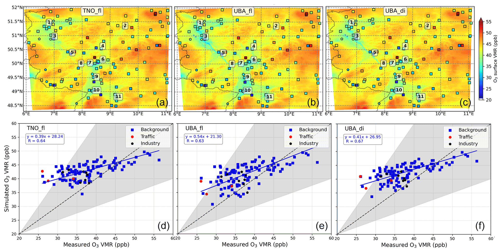
Figure B1Spatial distribution of monthly-mean O3 surface VMRs for the three simulations using different emission inventories (a, d: TNO, b, e: UBA without diurnal variations, c, f: UBA with diurnal variations) for May 2018. Panels (d), (e) and (f) show the scatter plot and orthogonal distance regression (ODR) weighted by the inverse of the square of the standard deviation of simulated monthly-mean O3 surface VMRs with respect to the in situ measured values. ODR was performed only for the background stations because of the low number of stations at the traffic-adjacent and industrial locations.
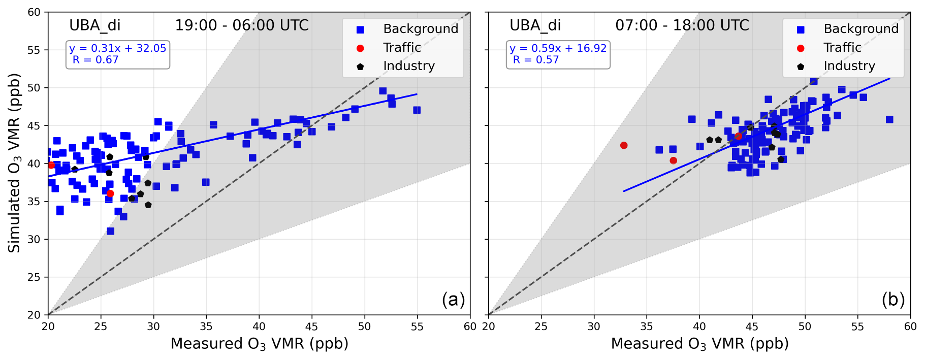
Figure B2Scatter plot between measured and simulated O3 for night-time (a) and daytime (b) for monthly means at all the measurement stations in the CM02 domain for the UBAdi set-up.
During night-time, we observe a general overestimation by ∼37 % for all the measurement stations combined. However, during daytime, we observed much better agreement with a relative bias of %. This indicates a relatively weaker amplitude of diurnal variability in the simulations. Mertens et al. (2016) have previously investigated the weak amplitude of simulated O3, such that night-time values are overestimated and that daytime values are represented well in a coarser resolution ( km2) MECO(n) simulation. They have shown that COSMO/MESSy diurnal profiles are related to that of the planetary boundary layer height (PBLH). MECO(n) simulates a relatively weaker-amplitude diurnal evolution of PBLH, such that the night-time values are biased high. This results in a large night-time “reservoir” of ozone that can undergo chemical titration with NOx or dry deposition. Furthermore, a stronger vertical mixing in COSMO/MESSy brings ozone-rich air, which together with a weaker dry deposition (Travis and Jacob, 2019) causes a positive bias in simulated surface ozone in the night-time. The stronger vertical mixing was also confirmed by Mertens et al. (2016) using a diagnostic tracer with no atmospheric sink. Over the European region, regional models usually struggle to capture the diurnal variability of surface O3 VMRs as indicated by AQMEII (Air Quality Model Evaluation International Initiative) studies (Solazzo et al., 2012; Im et al., 2015). For example, in WRF-CHEM, the night-time overestimation of surface O3 was found to be due to an underestimation of O3 titration by NOx in the night-time, while that in COSMO-MUSCAT was due to relatively weaker dry deposition fluxes and inaccurate representation of vertical mixing. A night-time overestimation over central Europe was also observed for global model EMAC, though the bias was smaller as compared to that in MECO(n) (Mertens et al., 2016). During the daytime, the cold bias of MECO(n) could also bias the rate of ozone production from precursors via rate constants. Mertens et al. (2016) have investigated this deviation by forcing the nudged EMAC-simulated temperatures in the COSMO/MESSy domain. This, however, did not explain the observed bias in O3.
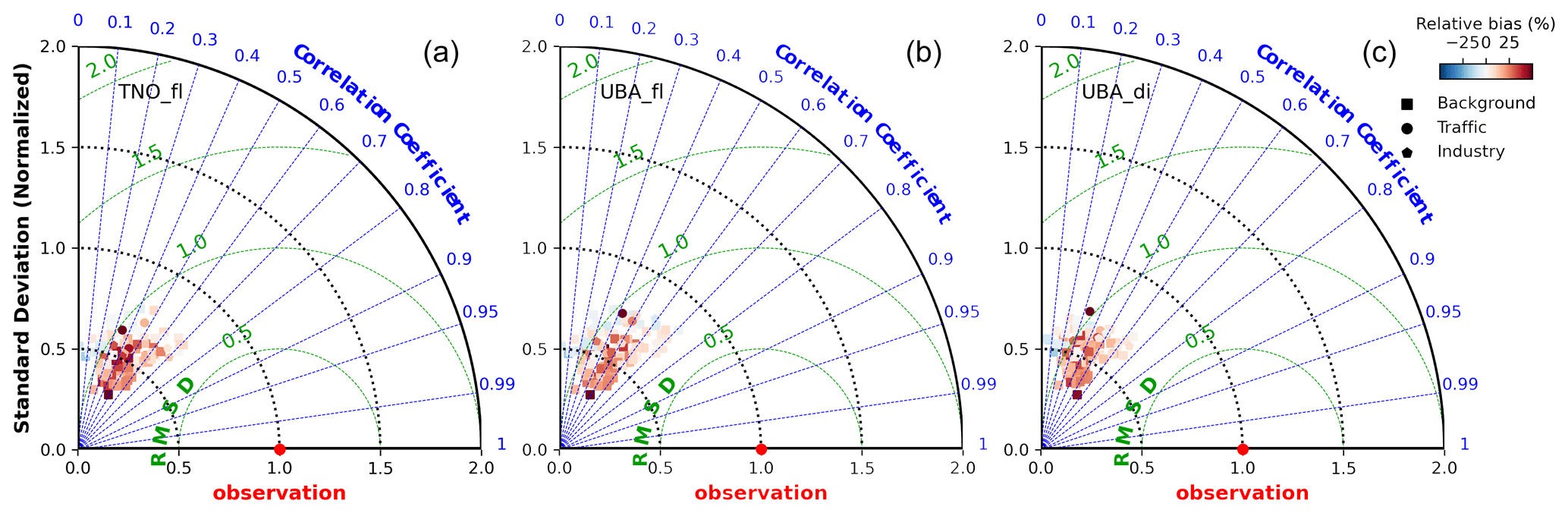
Figure B3Taylor diagrams showing the Pearson correlation coefficients, normalized standard deviation and normalized root mean square difference corresponding to hourly-resolved measured and simulated O3 VMRs (in CM02 domain) for background, traffic, and industrial sites represented as square, circle and pentagon markers, respectively. Panels (a), (b) and (c) correspond to the TNOfl, UBAfl and UBAdi set-ups, respectively.
The Taylor diagrams in Fig. B3 show significantly better model performance (larger R and smaller RMSD values) as compared to that for NO2 in Sect. 3.2. This is due to the relatively larger lifetime of O3, owing to which strong spatial gradients are not observed. The temporal variability is, however, underestimated as evident by the relative standard deviations of less than 1. Using an updated and highly resolved anthropogenic emission with high NOx did not elicit further improvement in the agreement of spatial patterns of the monthly-mean measured and simulated O3. The only improvement was a minor reduction in overestimation corresponding to the lower values. These values are observed for the sites where generally higher NO2 VMRs were observed, thus indicating a NOx saturated ozone production regime. It is interesting to note that an increase of ∼27 % anthropogenic NOx emissions by using the UBA emission inventory shows little change in surface O3 VMRs. In addition to the NOx saturated ozone production regime, a relatively weaker contribution of anthropogenic emissions towards the ozone production in summertime (Mertens et al., 2020b) could also be a plausible reason for this weak effect. However, there can be several discrepancies related to inappropriate NMVOC speciation, biogenic emissions and a relatively simpler chemical mechanism used in the model, due to which we are not confident about this finding. Further investigation in this direction is beyond the scope of this study and should be pursued in future work with complex chemistry.
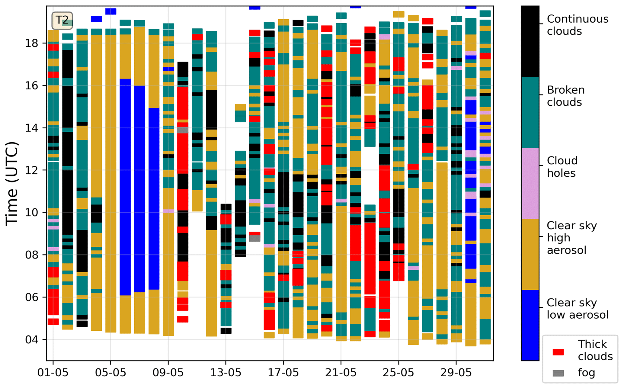
Figure C1Daily variability of the sky conditions for May 2018 retrieved using MAX-DOAS measurements along the azimuth direction of T2. Consistent sky conditions were retrieved for the other three azimuth directions
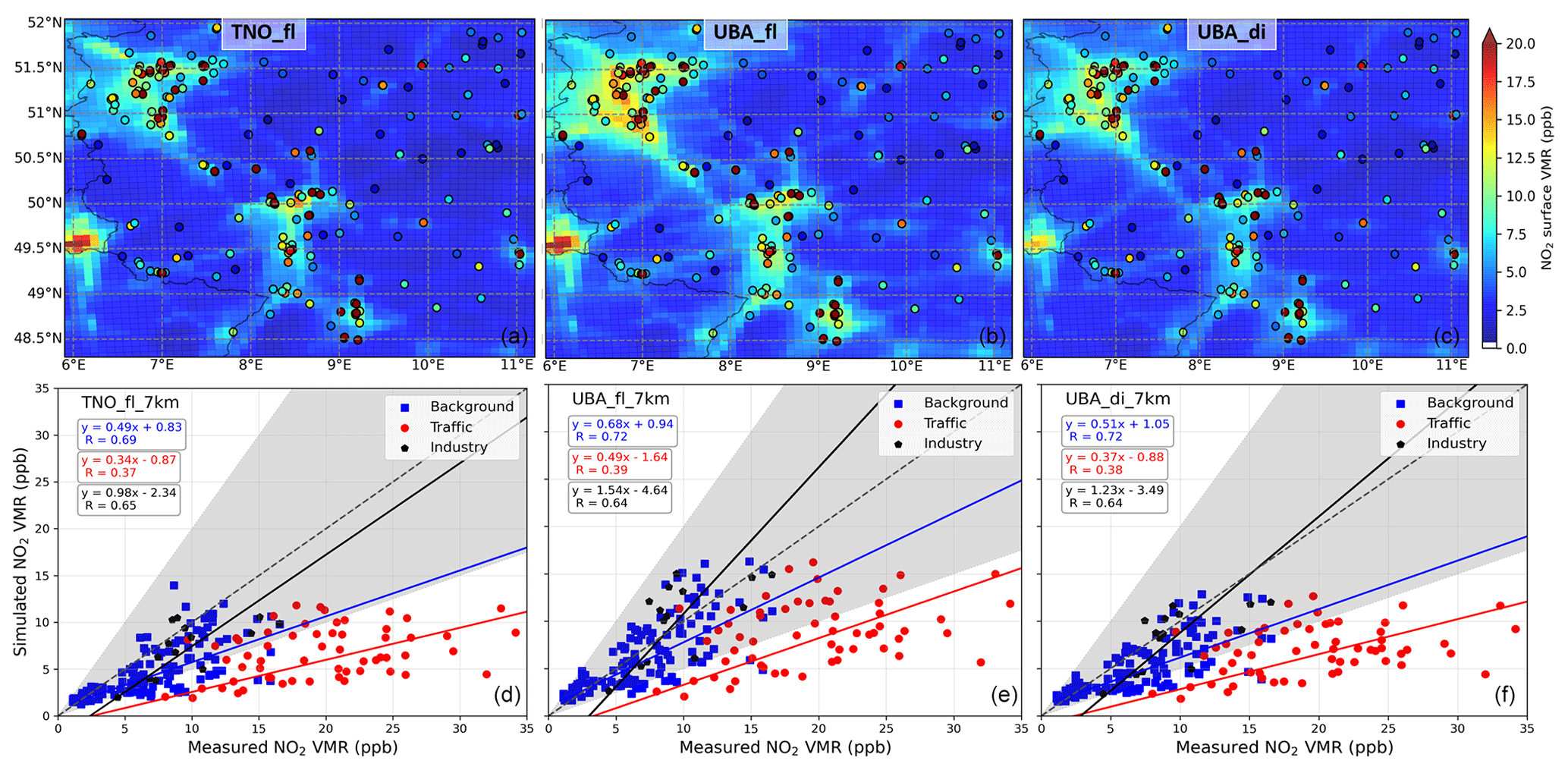
Figure C2Same as Fig. 4 but for the CM07 set-up in the domain limited to that for CM02 boundaries.
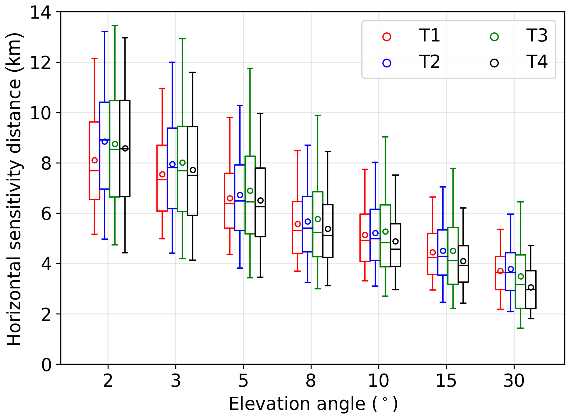
Figure C3Typical horizontal sensitivity distances (HSD) for different elevation angles along the viewing direction of the four telescopes. The HSD for an elevation angle α is estimated as the distance along the viewing direction which accounts for 90 % of simulated dSCDα.
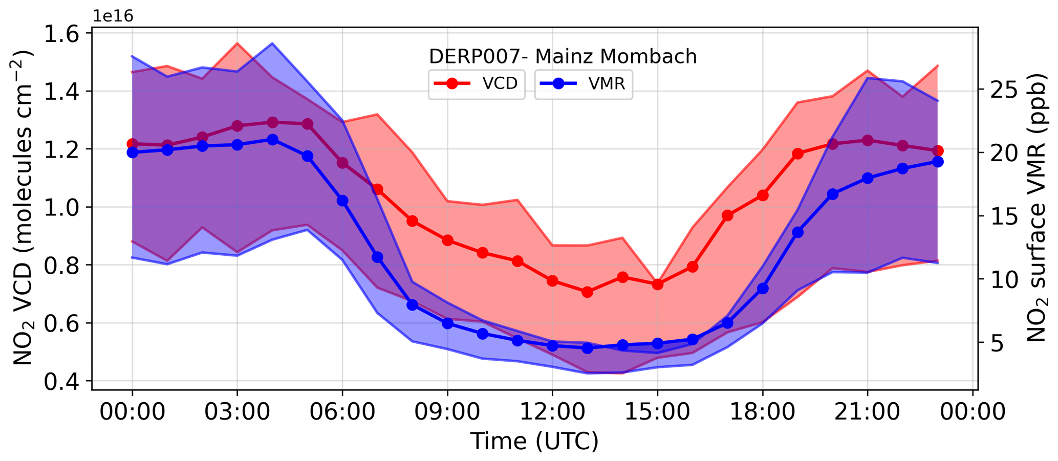
Figure C4Mean hourly diurnal profiles of simulated NO2 tropospheric VCDs (red) and surface volume mixing ratios (blue) at a background site (Mainz Mombach; 8.02∘ E, 50.02∘ N) for the model set-up UBAfl (diurnal variability of road transport and non-industrial combustion sectors not considered). The solid line and markers represent the mean, while the shaded region shows the inter-quartile variability range.
Table C1Fit settings chosen for MAX-DOAS spectral analyses.
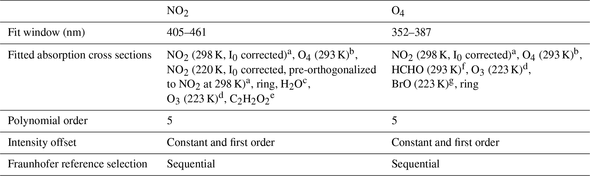
a Vandaele et al. (1998), b Thalman and Volkamer (2013), c Polyansky et al. (2018), d Bogumil et al. (2003), e Volkamer et al. (2005), f Meller and Moortgat (2000), g Fleischmann et al. (2004).
Table C2Summary of comparison of dSCDs (molecules cm−2) at various elevation angles for the three different model set-ups for the CM02 domain. The values in the brackets correspond to the RMSD, bias and R of the comparison of the geometric VCDs. The geometric dAMF at 30∘ elevation angle equals 1; hence, the geometric VCD is the same as the measured dSCD.

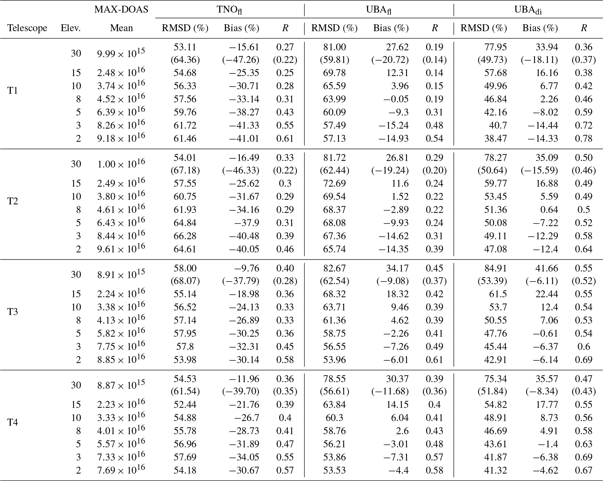
Modular Earth Submodel System (MESSy) is a multi-institutional project, and its license is available to the affiliates of these institutions. Affiliation to MESSy can be obtained by signing the MESSy Community End-User Licence Agreement (EULA) and accepting the MESSy Software Licence Agreement (SLA) available at https://www.messy-interface.org/ (last access: 13 July 2021, Jöckel et al., 2010, https://doi.org/10.5194/gmd-3-717-2010). The ECHAM5 model is available under the Software Licence Agreement of the Max Planck Institute for Meteorology, Hamburg. The COSMO model can be obtained either by institutional license provided by the German Meteorological Service (DWD) or individual license provided by the Climate Limited-area Modeling Community (CLM-Community). Further details about CLM-Community are available at https://wiki.coast.hzg.de/clmcom (last access: 13 July 2021, Rockel et al., 2008, https://doi.org/10.1127/0941-2948/2008/0309).
TNO MACC III emission data (Kuenen et al., 2014; https://doi.org/10.5194/acp-14-10963-2014) are provided by Jeroen J. P. Kuenen and Hugo A. C. Denier van der Gon at the TNO, Princetonlaan 6, 3584 CB Utrecht, the Netherlands, by signing the disclaimer and conditions for data use. The UBA anthropogenic emission data are made available by the German Environment Agency (Umweltbundesamt). Further details about the UBA emissions are available at https://www.umweltbundesamt.de/deutschland-karten-zu-luftschadstoff-daten (last access: 13 July 2021, UBA, 2021b). The hourly resolution measured data for NO2 and O3 are also provided by Umweltbundesamt and can be freely downloaded via the web interface https://www.umweltbundesamt.de/en/data/air/air-data/stations (last access: 13 July 2021, UBA, 2021a). The meteorological data used for model evaluation are provided by the German Meteorological Service (DWD) via the Climate Data Center web interface available at https://cdc.dwd.de/portal (last access: 13 July 2021, DWD, 2021).
VK and TW prepared the article with inputs from all the co-authors. JR performed the MAX-DOAS measurements and dSCD and dbAMF retrieval with inputs from SB and TW. AK, MM, BS, MB and HT helped VK with the model set-up and simulations. VK and AP pre-processed the TNO and UBA emission data so as to render them suitable for MECO(n). VK performed the cloud classification and data analyses related to model evaluation.
The authors declare that they have no conflict of interest.
Publisher’s note: Copernicus Publications remains neutral with regard to jurisdictional claims in published maps and institutional affiliations.
Vinod Kumar acknowledges the Max Planck Society and Alexander von Humboldt Foundation for providing financial support in the form of postdoctoral fellowship. We acknowledge the Umweltbundesamt and Deutscher Wetterdienst for in situ measurement data and UBA emission inventory. The model simulations were performed at the supercomputer MISTRAL of the German Climate Computing Centre. We thank Patrick Jöckel for maintenance and managing the license of the MESSy code. We thank Jeroen J. P. Kuenen for providing the TNO MACC III anthropogenic emission data and ECMWF for ERA-Interim reanalysis data used for nudging EMAC. Data analysis and visualization were performed using Python 3.8 and standard libraries including numpy, scipy, pandas, netCDF4, h5py, matplotlib, cartopy and geopy. We acknowledge the two anonymous reviewers for their constructive feedback on the article.
The article processing charges for this open-access publication were covered by the Max Planck Society.
This paper was edited by Folkert Boersma and reviewed by two anonymous referees.
Bechtold, P., Bazile, E., Guichard, F., Mascart, P., and Richard, E.: A mass-flux convection scheme for regional and global models, Q. J. Roy. Meteor. Soc., 127, 869–886, https://doi.org/10.1002/qj.49712757309, 2001. a
Beirle, S., Dörner, S., Donner, S., Remmers, J., Wang, Y., and Wagner, T.: The Mainz profile algorithm (MAPA), Atmos. Meas. Tech., 12, 1785–1806, https://doi.org/10.5194/amt-12-1785-2019, 2019. a
Blechschmidt, A.-M., Arteta, J., Coman, A., Curier, L., Eskes, H., Foret, G., Gielen, C., Hendrick, F., Marécal, V., Meleux, F., Parmentier, J., Peters, E., Pinardi, G., Piters, A. J. M., Plu, M., Richter, A., Segers, A., Sofiev, M., Valdebenito, Á. M., Van Roozendael, M., Vira, J., Vlemmix, T., and Burrows, J. P.: Comparison of tropospheric NO2 columns from MAX-DOAS retrievals and regional air quality model simulations, Atmos. Chem. Phys., 20, 2795–2823, https://doi.org/10.5194/acp-20-2795-2020, 2020. a, b, c, d, e
Boersma, K. F., Jacob, D. J., Eskes, H. J., Pinder, R. W., Wang, J., and van der A, R. J.: Intercomparison of SCIAMACHY and OMI tropospheric NO2 columns: Observing the diurnal evolution of chemistry and emissions from space, J. Geophys. Res., 113, D16S26, https://doi.org/10.1029/2007JD008816, 2008. a, b
Bogumil, K., Orphal, J., Homann, T., Voigt, S., Spietz, P., Fleischmann, O., Vogel, A., Hartmann, M., Kromminga, H., Bovensmann, H., Frerick, J., and Burrows, J.: Measurements of molecular absorption spectra with the SCIAMACHY pre-flight model: instrument characterization and reference data for atmospheric remote-sensing in the 230–2380 nm region, J. Photoch. Photobio. A, 157, 167–184, https://doi.org/10.1016/S1010-6030(03)00062-5, 2003. a
Böhm, U., Kücken, M., Ahrens, W., Block, A., Hauffe, D., Keuler, K., Rockel, B., and Will, A.: CLM–the climate version of LM: brief description and long-term applications, COSMO newsletter, 6, 225–235, 2006. a, b
Builtjes, P., van Loon, M., Schaap, M., Teeuwisse, S., Visschedijk, A., and Bloos, J.: The development of an emission data base over Europe and further contributions of TNO-MEP, Freie Universitaet Berlin/Institut fuer Meteorologie und Troposphaerischer Umweltforschung, Berlin, Germany, available at: https://www.umweltbundesamt.de/sites/default/files/medien/publikation/long/3607.pdf (last access: 13 July 2021), 2002. a, b, c
Chen, Y., Cheng, Y., Ma, N., Wei, C., Ran, L., Wolke, R., Größ, J., Wang, Q., Pozzer, A., Denier van der Gon, H. A. C., Spindler, G., Lelieveld, J., Tegen, I., Su, H., and Wiedensohler, A.: Natural sea-salt emissions moderate the climate forcing of anthropogenic nitrate, Atmos. Chem. Phys., 20, 771–786, https://doi.org/10.5194/acp-20-771-2020, 2020. a
Clémer, K., Van Roozendael, M., Fayt, C., Hendrick, F., Hermans, C., Pinardi, G., Spurr, R., Wang, P., and De Mazière, M.: Multiple wavelength retrieval of tropospheric aerosol optical properties from MAXDOAS measurements in Beijing, Atmos. Meas. Tech., 3, 863–878, https://doi.org/10.5194/amt-3-863-2010, 2010. a
Colette, A., Bessagnet, B., Meleux, F., Terrenoire, E., and Rouïl, L.: Frontiers in air quality modelling, Geosci. Model Dev., 7, 203–210, https://doi.org/10.5194/gmd-7-203-2014, 2014. a, b
Crippa, M., Guizzardi, D., Muntean, M., Schaaf, E., Dentener, F., van Aardenne, J. A., Monni, S., Doering, U., Olivier, J. G. J., Pagliari, V., and Janssens-Maenhout, G.: Gridded emissions of air pollutants for the period 1970–2012 within EDGAR v4.3.2, Earth Syst. Sci. Data, 10, 1987–2013, https://doi.org/10.5194/essd-10-1987-2018, 2018. a
Crippa, M., Solazzo, E., Huang, G., Guizzardi, D., Koffi, E., Muntean, M., Schieberle, C., Friedrich, R., and Janssens-Maenhout, G.: High resolution temporal profiles in the Emissions Database for Global Atmospheric Research, Scientific Data, 7, 121, https://doi.org/10.1038/s41597-020-0462-2, 2020. a, b
Deutschmann, T., Beirle, S., Frieß, U., Grzegorski, M., Kern, C., Kritten, L., Platt, U., Prados-Román, C., Puķīte, J., Wagner, T., Werner, B., and Pfeilsticker, K.: The Monte Carlo atmospheric radiative transfer model McArtim: Introduction and validation of Jacobians and 3D features, J. Quant. Spectrosc. Ra., 112, 1119–1137, https://doi.org/10.1016/j.jqsrt.2010.12.009, 2011. a
Dunlea, E. J., Herndon, S. C., Nelson, D. D., Volkamer, R. M., San Martini, F., Sheehy, P. M., Zahniser, M. S., Shorter, J. H., Wormhoudt, J. C., Lamb, B. K., Allwine, E. J., Gaffney, J. S., Marley, N. A., Grutter, M., Marquez, C., Blanco, S., Cardenas, B., Retama, A., Ramos Villegas, C. R., Kolb, C. E., Molina, L. T., and Molina, M. J.: Evaluation of nitrogen dioxide chemiluminescence monitors in a polluted urban environment, Atmos. Chem. Phys., 7, 2691–2704, https://doi.org/10.5194/acp-7-2691-2007, 2007. a
DWD: Yearbook 2019 of the Deutscher Wetterdienst, Deutscher Wetterdienst, available at: https://www.dwd.de/EN/ourservices/annual_reports_dwd/annual_reports_dwd.html (last access: 13 July 2021), 2019. a
DWD (German Meteorological Service): Climate Data Center, available at: https://cdc.dwd.de/portal, last access: 13 July 2021. a
EEA: Air quality in Europe – 2019 report, EEA Report No. 10/2019, 18–25, available at: https://www.eea.europa.eu//publications/air-quality-in-europe-2019 (last access: 13 July 2021), 2019. a
Eickelpasch, D. and Eickelpasch, G.: Determination and evaluation of ambient air quality-manual of ambient air monitoring in Germany, Umweltbundesamt, available at: https://www.umweltbundesamt.de/sites/default/files/medien/publikation/long/2702.pdf (last access: 13 July 2021), 2004. a
Fleischmann, O. C., Hartmann, M., Burrows, J. P., and Orphal, J.: New ultraviolet absorption cross-sections of BrO at atmospheric temperatures measured by time-windowing Fourier transform spectroscopy, J. Photoch. Photobio. A, 168, 117–132, https://doi.org/10.1016/j.jphotochem.2004.03.026, 2004. a
Frieß, U., Beirle, S., Alvarado Bonilla, L., Bösch, T., Friedrich, M. M., Hendrick, F., Piters, A., Richter, A., van Roozendael, M., Rozanov, V. V., Spinei, E., Tirpitz, J.-L., Vlemmix, T., Wagner, T., and Wang, Y.: Intercomparison of MAX-DOAS vertical profile retrieval algorithms: studies using synthetic data, Atmos. Meas. Tech., 12, 2155–2181, https://doi.org/10.5194/amt-12-2155-2019, 2019. a
Grewe, V.: Impact of Lightning on Air Chemistry and Climate, Springer Netherlands, Dordrecht, 537–549, https://doi.org/10.1007/978-1-4020-9079-0_25, 2009. a
Hofmann, C., Kerkweg, A., Wernli, H., and Jöckel, P.: The 1-way on-line coupled atmospheric chemistry model system MECO(n) – Part 3: Meteorological evaluation of the on-line coupled system, Geosci. Model Dev., 5, 129–147, https://doi.org/10.5194/gmd-5-129-2012, 2012. a
Hönninger, G., von Friedeburg, C., and Platt, U.: Multi axis differential optical absorption spectroscopy (MAX-DOAS), Atmos. Chem. Phys., 4, 231–254, https://doi.org/10.5194/acp-4-231-2004, 2004. a
Huang, G., Brook, R., Crippa, M., Janssens-Maenhout, G., Schieberle, C., Dore, C., Guizzardi, D., Muntean, M., Schaaf, E., and Friedrich, R.: Speciation of anthropogenic emissions of non-methane volatile organic compounds: a global gridded data set for 1970–2012, Atmos. Chem. Phys., 17, 7683–7701, https://doi.org/10.5194/acp-17-7683-2017, 2017. a
Ialongo, I., Virta, H., Eskes, H., Hovila, J., and Douros, J.: Comparison of TROPOMI/Sentinel-5 Precursor NO2 observations with ground-based measurements in Helsinki, Atmos. Meas. Tech., 13, 205–218, https://doi.org/10.5194/amt-13-205-2020, 2020. a
Im, U., Bianconi, R., Solazzo, E., Kioutsioukis, I., Badia, A., Balzarini, A., Baró, R., Bellasio, R., Brunner, D., Chemel, C., Curci, G., Flemming, J., Forkel, R., Giordano, L., Jiménez-Guerrero, P., Hirtl, M., Hodzic, A., Honzak, L., Jorba, O., Knote, C., Kuenen, J. J., Makar, P. A., Manders-Groot, A., Neal, L., Pérez, J. L., Pirovano, G., Pouliot, G., San Jose, R., Savage, N., Schroder, W., Sokhi, R. S., Syrakov, D., Torian, A., Tuccella, P., Werhahn, J., Wolke, R., Yahya, K., Zabkar, R., Zhang, Y., Zhang, J., Hogrefe, C., and Galmarini, S.: Evaluation of operational on-line-coupled regional air quality models over Europe and North America in the context of AQMEII phase 2. Part I: Ozone, Atmospheric Environment, 115, 404–420, https://doi.org/10.1016/j.atmosenv.2014.09.042, 2015. a
Jöckel, P., Tost, H., Pozzer, A., Brühl, C., Buchholz, J., Ganzeveld, L., Hoor, P., Kerkweg, A., Lawrence, M. G., Sander, R., Steil, B., Stiller, G., Tanarhte, M., Taraborrelli, D., van Aardenne, J., and Lelieveld, J.: The atmospheric chemistry general circulation model ECHAM5/MESSy1: consistent simulation of ozone from the surface to the mesosphere, Atmos. Chem. Phys., 6, 5067–5104, https://doi.org/10.5194/acp-6-5067-2006, 2006. a
Jöckel, P., Kerkweg, A., Pozzer, A., Sander, R., Tost, H., Riede, H., Baumgaertner, A., Gromov, S., and Kern, B.: Development cycle 2 of the Modular Earth Submodel System (MESSy2), Geosci. Model Dev., 3, 717–752, https://doi.org/10.5194/gmd-3-717-2010, 2010 (data available at: https://www.messy-interface.org/, last access: 13 July 2021). a, b, c
Kerkweg, A. and Jöckel, P.: The 1-way on-line coupled atmospheric chemistry model system MECO(n) – Part 2: On-line coupling with the Multi-Model-Driver (MMD), Geosci. Model Dev., 5, 111–128, https://doi.org/10.5194/gmd-5-111-2012, 2012a. a
Kerkweg, A. and Jöckel, P.: The 1-way on-line coupled atmospheric chemistry model system MECO(n) – Part 1: Description of the limited-area atmospheric chemistry model COSMO/MESSy, Geosci. Model Dev., 5, 87–110, https://doi.org/10.5194/gmd-5-87-2012, 2012b. a, b
Kerkweg, A. and Jöckel, P.: The infrastructure MESSy submodels GRID (v1.0) and IMPORT (v1.0), Geosci. Model Dev. Discuss., 8, 8607–8633, https://doi.org/10.5194/gmdd-8-8607-2015, 2015. a, b
Kerkweg, A., Buchholz, J., Ganzeveld, L., Pozzer, A., Tost, H., and Jöckel, P.: Technical Note: An implementation of the dry removal processes DRY DEPosition and SEDImentation in the Modular Earth Submodel System (MESSy), Atmos. Chem. Phys., 6, 4617–4632, https://doi.org/10.5194/acp-6-4617-2006, 2006a. a
Kerkweg, A., Sander, R., Tost, H., and Jöckel, P.: Technical note: Implementation of prescribed (OFFLEM), calculated (ONLEM), and pseudo-emissions (TNUDGE) of chemical species in the Modular Earth Submodel System (MESSy), Atmos. Chem. Phys., 6, 3603–3609, https://doi.org/10.5194/acp-6-3603-2006, 2006b. a, b, c
Kerkweg, A., Hofmann, C., Jöckel, P., Mertens, M., and Pante, G.: The on-line coupled atmospheric chemistry model system MECO(n) – Part 5: Expanding the Multi-Model-Driver (MMD v2.0) for 2-way data exchange including data interpolation via GRID (v1.0), Geosci. Model Dev., 11, 1059–1076, https://doi.org/10.5194/gmd-11-1059-2018, 2018. a
Kuenen, J. J. P., Visschedijk, A. J. H., Jozwicka, M., and Denier van der Gon, H. A. C.: TNO-MACC_II emission inventory; a multi-year (2003–2009) consistent high-resolution European emission inventory for air quality modelling, Atmos. Chem. Phys., 14, 10963–10976, https://doi.org/10.5194/acp-14-10963-2014, 2014. a, b, c, d
Kuik, F., Kerschbaumer, A., Lauer, A., Lupascu, A., von Schneidemesser, E., and Butler, T. M.: Top–down quantification of NOx emissions from traffic in an urban area using a high-resolution regional atmospheric chemistry model, Atmos. Chem. Phys., 18, 8203–8225, https://doi.org/10.5194/acp-18-8203-2018, 2018. a, b, c, d
Kumar, V., Beirle, S., Dörner, S., Mishra, A. K., Donner, S., Wang, Y., Sinha, V., and Wagner, T.: Long-term MAX-DOAS measurements of NO2, HCHO, and aerosols and evaluation of corresponding satellite data products over Mohali in the Indo-Gangetic Plain, Atmos. Chem. Phys., 20, 14183–14235, https://doi.org/10.5194/acp-20-14183-2020, 2020. a
Liu, M., Lin, J., Kong, H., Boersma, K. F., Eskes, H., Kanaya, Y., He, Q., Tian, X., Qin, K., Xie, P., Spurr, R., Ni, R., Yan, Y., Weng, H., and Wang, J.: A new TROPOMI product for tropospheric NO2 columns over East Asia with explicit aerosol corrections, Atmos. Meas. Tech., 13, 4247–4259, https://doi.org/10.5194/amt-13-4247-2020, 2020. a
Meller, R. and Moortgat, G. K.: Temperature dependence of the absorption cross sections of formaldehyde between 223 and 323 K in the wavelength range 225–375 nm, J. Geophys. Res., 105, 7089–7101, https://doi.org/10.1029/1999jd901074, 2000. a
Mertens, M., Kerkweg, A., Jöckel, P., Tost, H., and Hofmann, C.: The 1-way on-line coupled model system MECO(n) – Part 4: Chemical evaluation (based on MESSy v2.52), Geosci. Model Dev., 9, 3545–3567, https://doi.org/10.5194/gmd-9-3545-2016, 2016. a, b, c, d, e, f, g, h, i
Mertens, M., Kerkweg, A., Grewe, V., Jöckel, P., and Sausen, R.: Are contributions of emissions to ozone a matter of scale? – a study using MECO(n) (MESSy v2.50), Geosci. Model Dev., 13, 363–383, https://doi.org/10.5194/gmd-13-363-2020, 2020a. a, b
Mertens, M., Kerkweg, A., Grewe, V., Jöckel, P., and Sausen, R.: Attributing ozone and its precursors to land transport emissions in Europe and Germany, Atmos. Chem. Phys., 20, 7843–7873, https://doi.org/10.5194/acp-20-7843-2020, 2020b. a
Minkos, A., Dauert, U., Feigenspan, S., and Kessinger, S.: Air Quality 2019 Preliminary Evaluation, Umweltbundesamt, Dessau-Roßlau, Germany, available at: https://www.umweltbundesamt.de/publikationen/luftqualitaet-2018 (last access: 13 July 2021), 2019. a
Miyazaki, K., Eskes, H. J., and Sudo, K.: Global NOx emission estimates derived from an assimilation of OMI tropospheric NO2 columns, Atmos. Chem. Phys., 12, 2263–2288, https://doi.org/10.5194/acp-12-2263-2012, 2012. a
Platt, U. and Stutz, J.: Differential Optical Absorption Spectroscopy, Springer, Berlin, Heidelberg, Vol. XVI, https://doi.org/10.1007/978-3-540-75776-4, 2008. a
Polyansky, O. L., Kyuberis, A. A., Zobov, N. F., Tennyson, J., Yurchenko, S. N., and Lodi, L.: ExoMol molecular line lists XXX: a complete high-accuracy line list for water, Mon. Not. R. Astron. Soc., 480, 2597–2608, https://doi.org/10.1093/mnras/sty1877, 2018. a
Pozzer, A., Jöckel, P., and Van Aardenne, J.: The influence of the vertical distribution of emissions on tropospheric chemistry, Atmos. Chem. Phys., 9, 9417–9432, https://doi.org/10.5194/acp-9-9417-2009, 2009. a, b
Pöschl, U., von Kuhlmann, R., Poisson, N., and Crutzen, P. J.: Development and Intercomparison of Condensed Isoprene Oxidation Mechanisms for Global Atmospheric Modeling, J. Atmos. Chem., 37, 29–52, https://doi.org/10.1023/A:1006391009798, 2000. a
Remmers, J.: Spatial distribution of trace gases and aerosols in the troposphere, PhD thesis, Johannes Gutenberg-Universität Mainz, Germany, 2021. a
Rockel, B., Will, A., and Hense, A.: The Regional Climate Model COSMO-CLM (CCLM), Meteorol. Z., 17, 347–348, https://doi.org/10.1127/0941-2948/2008/0309, 2008 (data available at: https://wiki.coast.hzg.de/clmcom, last access: 13 July 2021). a, b, c
Roeckner, E., Bäuml, G., Bonaventura, L., Brokopf, R., Esch, M., Giorgetta, M., Hagemann, S., Kirchner, I., Kornblueh, L., and Manzini, E.: The atmospheric general circulation model ECHAM 5. PART I: Model description, Report No. 349, Max-Planck-Institut für Meteorologie, available at: http://hdl.handle.net/11858/00-001M-0000-0012-0144-5 (last access: 13 July 2021), 2003. a
Sander, R., Jöckel, P., Kirner, O., Kunert, A. T., Landgraf, J., and Pozzer, A.: The photolysis module JVAL-14, compatible with the MESSy standard, and the JVal PreProcessor (JVPP), Geosci. Model Dev., 7, 2653–2662, https://doi.org/10.5194/gmd-7-2653-2014, 2014. a
Schaap, M., Roemer, M., Sauter, F., Boersen, G., Timmermans, R., Builtjes, P., and Vermeulen, A.: Lotos-euros: Documentation, TNO report B&O-A, 297, TNO, The Netherlands, available at: https://wdc.dlr.de/data_products/projects/promote/IAQ/Documentation-LOTOS-2005-297.pdf (last access: 13 July 2021), 2005. a, b, c, d, e
Schaap, M., Cuvelier, C., Hendriks, C., Bessagnet, B., Baldasano, J., Colette, A., Thunis, P., Karam, D., Fagerli, H., Graff, A., Kranenburg, R., Nyiri, A., Pay, M., Rouïl, L., Schulz, M., Simpson, D., Stern, R., Terrenoire, E., and Wind, P.: Performance of European chemistry transport models as function of horizontal resolution, Atmos. Environ., 112, 90–105, https://doi.org/10.1016/j.atmosenv.2015.04.003, 2015. a
Shaiganfar, R., Beirle, S., Sharma, M., Chauhan, A., Singh, R. P., and Wagner, T.: Estimation of NOx emissions from Delhi using Car MAX-DOAS observations and comparison with OMI satellite data, Atmos. Chem. Phys., 11, 10871–10887, https://doi.org/10.5194/acp-11-10871-2011, 2011. a
Shaiganfar, R., Beirle, S., Petetin, H., Zhang, Q., Beekmann, M., and Wagner, T.: New concepts for the comparison of tropospheric NO2 column densities derived from car-MAX-DOAS observations, OMI satellite observations and the regional model CHIMERE during two MEGAPOLI campaigns in Paris 2009/10, Atmos. Meas. Tech., 8, 2827–2852, https://doi.org/10.5194/amt-8-2827-2015, 2015. a, b
Solazzo, E., Bianconi, R., Vautard, R., Appel, K. W., Moran, M. D., Hogrefe, C., Bessagnet, B., Brandt, J., Christensen, J. H., Chemel, C., Coll, I., Denier van der Gon, H., Ferreira, J., Forkel, R., Francis, X. V., Grell, G., Grossi, P., Hansen, A. B., Jeričević, A., Kraljević, L., Miranda, A. I., Nopmongcol, U., Pirovano, G., Prank, M., Riccio, A., Sartelet, K. N., Schaap, M., Silver, J. D., Sokhi, R. S., Vira, J., Werhahn, J., Wolke, R., Yarwood, G., Zhang, J., Rao, S., and Galmarini, S.: Model evaluation and ensemble modelling of surface-level ozone in Europe and North America in the context of AQMEII, Atmos. Environ., 53, 60–74, https://doi.org/10.1016/j.atmosenv.2012.01.003, 2012. a
Solazzo, E., Crippa, M., Guizzardi, D., Muntean, M., Choulga, M., and Janssens-Maenhout, G.: Uncertainties in the Emissions Database for Global Atmospheric Research (EDGAR) emission inventory of greenhouse gases, Atmos. Chem. Phys., 21, 5655–5683, https://doi.org/10.5194/acp-21-5655-2021, 2021. a
Steppeler, J., Doms, G., Schättler, U., Bitzer, H. W., Gassmann, A., Damrath, U., and Gregoric, G.: Meso-gamma scale forecasts using the nonhydrostatic model LM, Meteorol. Atmos. Phys., 82, 75–96, https://doi.org/10.1007/s00703-001-0592-9, 2003. a
Strogies, M., Gniffke, P., and Hausmann, K.: German Informative Inventory Report 2020, Report, Umweltbundesamt, Dessau-Roßlau, Germany, available at: http://iir-de-2020.wikidot.com/summary (last access: 13 July 2021), 2020. a
Taylor, K. E.: Summarizing multiple aspects of model performance in a single diagram, J. Geophys. Res., 106, 7183–7192, https://doi.org/10.1029/2000JD900719, 2001. a
Thalman, R. and Volkamer, R.: Temperature dependent absorption cross-sections of collision pairs between 340 and 630 nm and at atmospherically relevant pressure, Phys. Chem. Chem. Phys., 15, 15371–15381, https://doi.org/10.1039/C3CP50968K, 2013. a
Tiedtke, M.: A Comprehensive Mass Flux Scheme for Cumulus Parameterization in Large-Scale Models, Mon. Weather Rev., 117, 1779–1800, https://doi.org/10.1175/1520-0493(1989)117<1779:ACMFSF>2.0.CO;2, 1989. a
Tost, H., Jöckel, P., Kerkweg, A., Sander, R., and Lelieveld, J.: Technical note: A new comprehensive SCAVenging submodel for global atmospheric chemistry modelling, Atmos. Chem. Phys., 6, 565–574, https://doi.org/10.5194/acp-6-565-2006, 2006. a, b
Tost, H., Lawrence, M. G., Brühl, C., Jöckel, P., The GABRIEL Team, and The SCOUT-O3-DARWIN/ACTIVE Team: Uncertainties in atmospheric chemistry modelling due to convection parameterisations and subsequent scavenging, Atmos. Chem. Phys., 10, 1931–1951, https://doi.org/10.5194/acp-10-1931-2010, 2010. a
Travis, K. R. and Jacob, D. J.: Systematic bias in evaluating chemical transport models with maximum daily 8 h average (MDA8) surface ozone for air quality applications: a case study with GEOS-Chem v9.02, Geosci. Model Dev., 12, 3641–3648, https://doi.org/10.5194/gmd-12-3641-2019, 2019. a
Travis, K. R., Jacob, D. J., Fisher, J. A., Kim, P. S., Marais, E. A., Zhu, L., Yu, K., Miller, C. C., Yantosca, R. M., Sulprizio, M. P., Thompson, A. M., Wennberg, P. O., Crounse, J. D., St. Clair, J. M., Cohen, R. C., Laughner, J. L., Dibb, J. E., Hall, S. R., Ullmann, K., Wolfe, G. M., Pollack, I. B., Peischl, J., Neuman, J. A., and Zhou, X.: Why do models overestimate surface ozone in the Southeast United States?, Atmos. Chem. Phys., 16, 13561–13577, https://doi.org/10.5194/acp-16-13561-2016, 2016. a
UBA (Umweltbundesamt – German Environment Agency): Current air data, UBA [data set], available at: https://www.umweltbundesamt.de/en/data/air/air-data/stations, last access: 13 July 2021a. a
UBA (Umweltbundesamt – German Environment Agency): Deutschland-Karten zu Luftschadstoff-Daten, UBA [data set], available at: https://www.umweltbundesamt.de/deutschland-karten-zu-luftschadstoff-daten, last access: 13 July 2021b (in German). a
Valin, L. C., Russell, A. R., Hudman, R. C., and Cohen, R. C.: Effects of model resolution on the interpretation of satellite NO2 observations, Atmos. Chem. Phys., 11, 11647–11655, https://doi.org/10.5194/acp-11-11647-2011, 2011. a
Vandaele, A. C., Hermans, C., Simon, P. C., Carleer, M., Colin, R., Fally, S., Mérienne, M. F., Jenouvrier, A., and Coquart, B.: Measurements of the NO2 absorption cross-section from 42 000 cm−1 to 10 000 cm−1 (238–1000 nm) at 220 K and 294 K, J. Quant. Spectrosc. Ra., 59, 171–184, https://doi.org/10.1016/S0022-4073(97)00168-4, 1998. a
Veefkind, J., Aben, I., McMullan, K., Förster, H., de Vries, J., Otter, G., Claas, J., Eskes, H., de Haan, J., Kleipool, Q., van Weele, M., Hasekamp, O., Hoogeveen, R., Landgraf, J., Snel, R., Tol, P., Ingmann, P., Voors, R., Kruizinga, B., Vink, R., Visser, H., and Levelt, P.: TROPOMI on the ESA Sentinel-5 Precursor: A GMES mission for global observations of the atmospheric composition for climate, air quality and ozone layer applications, Remote Sens. Environ., 120, 70–83, https://doi.org/10.1016/j.rse.2011.09.027, 2012. a
Vinken, G. C. M., Boersma, K. F., van Donkelaar, A., and Zhang, L.: Constraints on ship NOx emissions in Europe using GEOS-Chem and OMI satellite NO2 observations, Atmos. Chem. Phys., 14, 1353–1369, https://doi.org/10.5194/acp-14-1353-2014, 2014. a
Visser, A. J., Boersma, K. F., Ganzeveld, L. N., and Krol, M. C.: European NOx emissions in WRF-Chem derived from OMI: impacts on summertime surface ozone, Atmos. Chem. Phys., 19, 11821–11841, https://doi.org/10.5194/acp-19-11821-2019, 2019. a, b, c
Vlemmix, T., Eskes, H. J., Piters, A. J. M., Schaap, M., Sauter, F. J., Kelder, H., and Levelt, P. F.: MAX-DOAS tropospheric nitrogen dioxide column measurements compared with the Lotos-Euros air quality model, Atmos. Chem. Phys., 15, 1313–1330, https://doi.org/10.5194/acp-15-1313-2015, 2015. a, b, c, d
Volkamer, R., Molina, L. T., Molina, M. J., Shirley, T., and Brune, W. H.: DOAS measurement of glyoxal as an indicator for fast VOC chemistry in urban air, Geophys. Res. Lett., 32, L08806, https://doi.org/10.1029/2005GL022616, 2005. a
Wagner, T., Dix, B., Friedeburg, C. v., Frieß, U., Sanghavi, S., Sinreich, R., and Platt, U.: MAX-DOAS O4 measurements: A new technique to derive information on atmospheric aerosols–Principles and information content, J. Geophys. Res., 109, D22205, https://doi.org/10.1029/2004JD004904, 2004. a
Wagner, T., Beirle, S., Brauers, T., Deutschmann, T., Frieß, U., Hak, C., Halla, J. D., Heue, K. P., Junkermann, W., Li, X., Platt, U., and Pundt-Gruber, I.: Inversion of tropospheric profiles of aerosol extinction and HCHO and NO2 mixing ratios from MAX-DOAS observations in Milano during the summer of 2003 and comparison with independent data sets, Atmos. Meas. Tech., 4, 2685–2715, https://doi.org/10.5194/amt-4-2685-2011, 2011. a
Wagner, T., Beirle, S., Remmers, J., Shaiganfar, R., and Wang, Y.: Absolute calibration of the colour index and O4 absorption derived from Multi AXis (MAX-)DOAS measurements and their application to a standardised cloud classification algorithm, Atmos. Meas. Tech., 9, 4803–4823, https://doi.org/10.5194/amt-9-4803-2016, 2016. a
- Abstract
- Introduction
- Methods
- Results and discussion
- Conclusions
- Appendix A: Temporal profiles and sector contributions of emissions
- Appendix B: Evaluation of surface mixing ratios of O3
- Appendix C: Additional figures and tables
- Code availability
- Data availability
- Author contributions
- Competing interests
- Disclaimer
- Acknowledgements
- Financial support
- Review statement
- References