Airborne Mid-Infrared Cavity enhanced Absorption spectrometer (AMICA)

We describe the Airborne Mid-Infrared Cavity enhanced Absorption spectrometer (AMICA) designed to measure trace gases in situ on research aircraft using Off-Axis Integrated Cavity Output Spectroscopy (OA-ICOS). AMICA contains two largely independent and exchangeable OA-ICOS arrangements, allowing for the simultaneous measurement of multiple substances in different infrared wavelength windows tailored to scientific questions related to a particular flight mission. Three OA-ICOS setups have been implemented with the aim to measure OCS, CO₂, CO, and H₂O at 2050 cm⁻¹; O₃, NH₃, and CO₂ at 1034 cm⁻¹; and HCN, C₂H₂, and N₂O at 3331 cm⁻¹. The 2050 cm⁻¹ setup has been characterized in the laboratory and successfully used for atmospheric measurements during two campaigns with the research aircraft M55 Geophysica and one with the German HALO (High Altitude and Long Range Research Aircraft). For OCS and CO, data for scientific use have been produced with 5 % accuracy (15 % for CO below 60 ppb, due to additional uncertainties introduced by dilution of the standard) at typical atmospheric mixing ratios and laboratory-measured 1σ precision of 30 ppt for OCS and 3 ppb for CO at 0.5 Hz time resolution. For CO₂, high absorption at atmospheric mixing ratios leads to saturation effects that limit sensitivity and complicate the spectral analysis, resulting in too large uncertainties for scientific use. For H₂O, absorption is too weak to be measured at mixing ratios below 100 ppm. By further reducing electrical noise and improving the treatment of the baseline in the spectral retrieval, we hope to improve precision for OCS and CO, resolve the issues inhibiting useful CO₂ measurements, and lower the detection limit for H₂O. The 1035 and 3331 cm⁻¹ arrangements have only partially been characterized and are still in development. Although both setups have been flown and recorded infrared spectra during field campaigns, no data for scientific use have yet been produced due to unresolved deviations of the retrieved mixing ratios to known standards (O₃) or insufficient sensitivity (NH₃, HCN, C₂H₂, N₂O). The ∼100 kg instrument with a typical in-flight power consumption of about 500 VA is dimensioned to fit into one 19 in. rack typically used for deployment inside the aircraft cabin. Its rugged design and a pressurized and temperature-stabilized compartment containing the sensitive optical and electronic hardware also allow for deployment in payload bays outside the pressurized cabin even at high altitudes of 20 km. A sample flow system with two parallel proportional solenoid valves of different size orifices allows for precise regulation of cavity pressure over the wide range of inlet port pressures encountered between the ground and maximum flight altitudes. Sample flow of the order of 1 SLM (standard litre per minute) maintained by an exhaust-side pump limits the useful time resolution to about 2.5 s (corresponding to the average cavity flush time), equivalent to 500 m distance at a typical aircraft speed of 200 m s⁻¹.

1 Introduction

Airborne in situ trace gas observations are typically made at high spatial and temporal resolutions and thus allow for the investigation of small- and intermediate-scale processes (e.g. Schumann et al., 2013). Most important trace gases possess reasonably strong absorption bands in the infrared region, so infrared absorption spectroscopy offers a simple and straightforward measurement technique for many gases. Measurement sensitivity critically depends on path length, and many trace gases at atmospheric abundances can only be detected with path lengths of hundreds of metres or even several kilometres. With in situ instruments, the long path lengths needed are often beyond those offered by common multi-pass cells (e.g. Robert, 2007; Herriott and Schulte, 1965; White, 1942) and are accessible only by using cavity-enhanced methods where path lengths of many kilometres can be achieved with mirrors of sufficient reflectivity. Those methods all go back to the cavity ring-down spectroscopy first described by O'Keefe and Deacon (1988). A wide variety of modifications and offsprings of this original technique have been developed and used for many different applications over the past 3 decades. Reviews with a historical overview of cavity-enhanced spectroscopy and a comprehensive listing of available methods have been given by Paldus and Kachanov (2005) and more recently by Gagliardi and Loock (2014).

Cavity-enhanced spectrometers in the near-infrared and mid-infrared region are commercially available for numerous trace gases. A cavity-enhanced technique that is sensitive, robust and easy to implement is the Off-Axis Integrated Cavity Output Spectroscopy (OA-ICOS; Baer et al., 2002; O'Keefe, 1998; O'Keefe et al., 1999; Paul et al., 2001). OA-ICOS has become a well-established technique for ground-based measurements of a wide range of trace gases, e.g. CO, N₂O, CH₄, CO₂ and water isotopes (e.g. Arévalo-Martinez et al., 2013; Hendriks et al., 2008; Kurita et al., 2012; Steen-Larsen et al., 2013). OA-ICOS measurements on research aircraft have been made (Leen et al., 2013; O'Shea et al., 2013; Provencal et al., 2005; Sayres et al., 2009), but these instruments often rely on the instrument being placed inside a pressurized cabin and/or need inverters to reduce the frequency of the electrical power generated by the aircraft's engines from the typical 400 Hz down to the more common 50 or 60 Hz.

The Airborne Mid-Infrared Cavity enhanced Absorption spectrometer (AMICA) is a novel two-cavity airborne OA-ICOS analyser simultaneously measuring multiple trace gases. The initial choice of gases during the instrument development has been driven by the research group's scientific interest and objectives of initially planned missions. One trace gas of interest is carbonyl sulfide (OCS), the most stable and abundant reduced sulfur gas in the atmosphere and a precursor to stratospheric sulfate aerosol (Crutzen, 1976; Kremser et al., 2016) as well as a potential tracer for the important carbon cycle process of net primary production (Whelan et al., 2018). Using a prototype of both AMICA and the commercially available Los Gatos OCS analyser measuring near 2050 cm⁻¹, OCS measurements have been conducted during field campaigns since 2014 mainly on research ships (Lennartz et al., 2017, 2020). In the wavelength region of the major OCS band in the infrared, carbon monoxide (CO), carbon dioxide (CO₂) and water vapour (H₂O) also absorb and are measured simultaneously by these analysers. The attempt to measure hydrogen cyanide (HCN) and acetylene (C₂H₂) near 3332 cm⁻¹ (where nitrous oxide, N₂O, also absorbs and can potentially be measured as an add-on) was motivated by their use as biomass burning tracers in the context of OCS (Notholt et al., 2003) and as pollution tracers in the Asian monsoon anticyclone (Park et al., 2008; Randel et al., 2010), the region of interest of two recent aircraft missions described further below. A cavity setup equivalent to the Los Gatos ammonia (NH₃) analyser in the 1034 cm⁻¹ region was tested to measure ozone (O₃), which is abundant in stratospheric air expected to be sampled at high altitudes.

A first operational version of AMICA for laboratory tests was completed in February 2016, and the first airborne deployment took place in August 2016. Since then, AMICA has evolved as corrections and upgrades were implemented based on the results from tests and deployments. In this paper, we describe the latest and current version of AMICA that has been optimized both in terms of reliability and performance. Where earlier laboratory and field data from AMICA are presented, appropriate reference to differences in the setup and hardware used will be made. In Sect. 2 we describe the special design features that ensure AMICA can function optimally on a moving and vibrating aircraft at pressures and temperatures down to 50 hPa and −80 ^∘C respectively. Section 2 also includes a detailed description of the implementation of OA-ICOS in AMICA. Details on data handling and analysis are given in Sect. 3. Realized cavity setups at certain wavelength windows in the infrared aiming at the abovementioned target species are described in Sect. 4 that also includes results from laboratory tests and calibrations. Finally, in Sect. 5, the first airborne measurements that demonstrate AMICA's functionality, performance and potential are presented.

2 Instrument design and description

2.1 General setup and bulk characteristics

Figure 1 shows a 3D technical drawing of AMICA. It consists of two main compartments: the main ICOS enclosure containing two OA-ICOS cavities with their respective laser and data acquisition hardware and electronics (Sect. 2.2) and an attached powerbox containing electrical components converting the AC supply input voltage to various filtered DC voltages (Sect. 2.5). A single stream of sampling air is drawn serially through two cavities, maintaining a constant pressure in each cavity (Sect. 2.4). Safe aircraft deployment is ensured by a robust design, with numerous features to withstand significant vibrational stress as well as severe pressure and temperature conditions (Sect. 2.3), and by an electronic design and grounding concept minimizing interference with the aircraft and other instruments (Sect. 2.5).

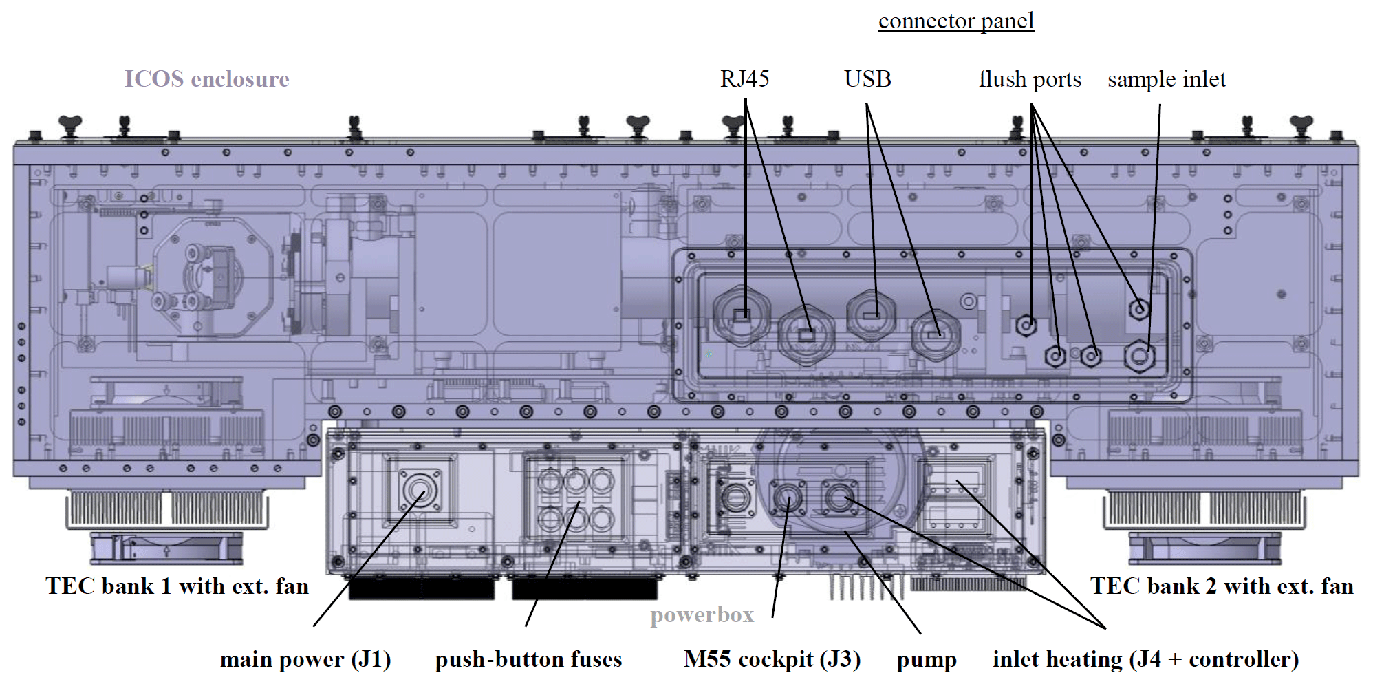
Figure 1 Technical drawing of AMICA showing bulk parts. Additional drawings including M55 mounts and the HALO rack are given in Figs. S1 and S2 in the Supplement respectively.

Table 1 Dimensions, weights and power draw of AMICA itemized for different parts and for the two different aircraft configurations. Note that TEC is thermoelectric cooler.

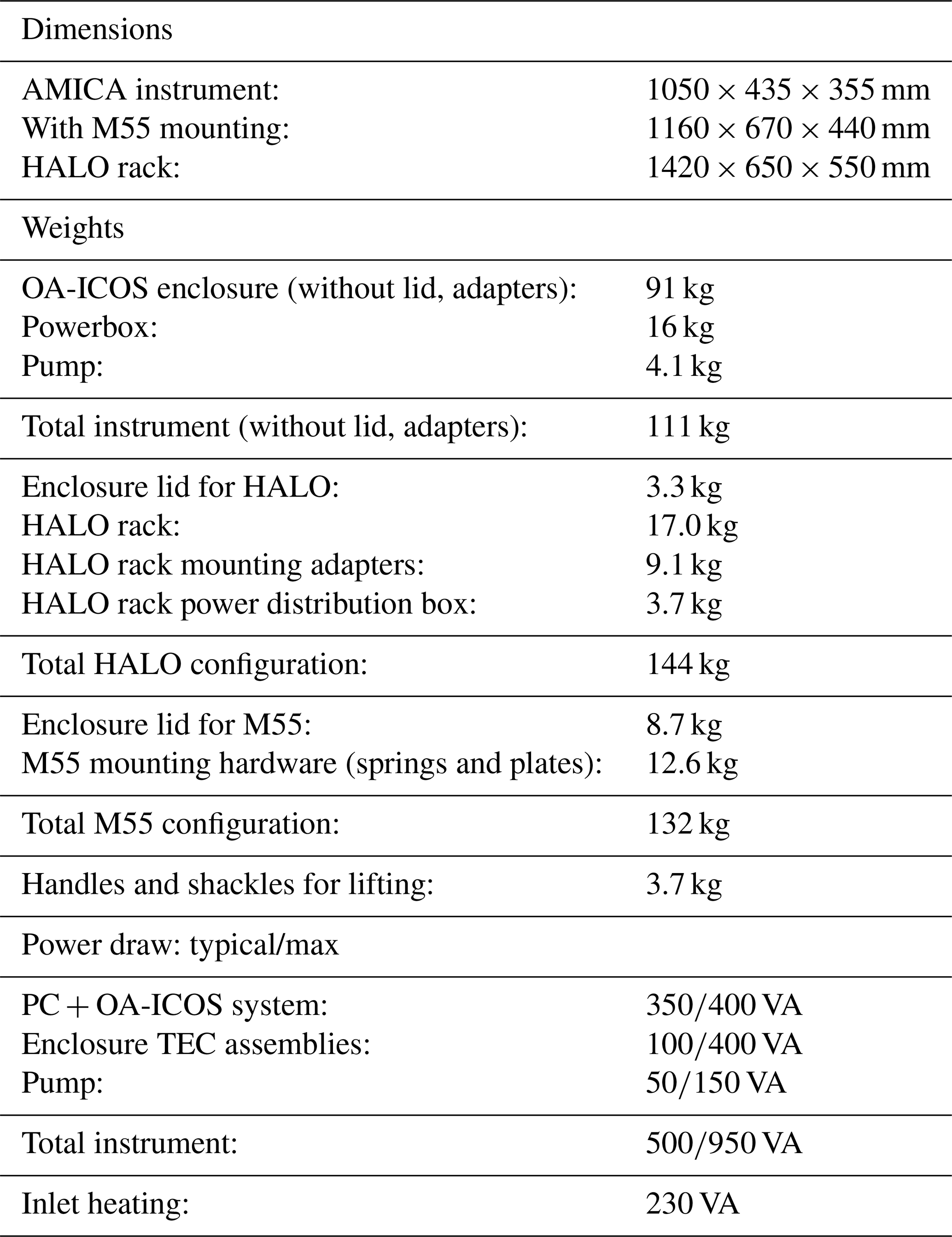
Not including aircraft-specific rack or mounting hardware (Sect. 2.3), the dimensions are $\mathrm{1050}\times \mathrm{435}\times \mathrm{355}$ mm, and the weight is approximately 115 kg. The power consumption is up to 800 VA at start-up and during the initial warm-up phase (taking between 2 and 45 min depending on ambient conditions), and typically 500 VA during normal operation of the warmed-up instrument. An additional 230 VA can be passed through AMICA to supply power to a heated inlet when this is needed (cf. Sect. 2.5). More detailed information with itemized weights and power characteristics is given in Table 1.

2.2 ICOS implementation

AMICA contains two largely independent OA-ICOS systems in a pressurized and temperature-stabilized enclosure (cf. Sect. 2.3). The arrangement of the different components can be seen in Fig. 2. Each ICOS entity consists of a laser source (C7 in Fig. 2 and Table 2), a 25.4 mm diameter round 90^∘ deflection mirror with a protected silver coating, a 508 mm long cavity of 48 mm inner diameter with two 50.8 mm diameter concave high-reflectivity mirrors with a 1 m radius of curvature (ABB Inc.), a 50.8 mm diameter 25 mm focal length aspheric/plano collimating lens (ZnSe for the 1034 and 2050 cm⁻¹ channels, Ge for the 3331 cm⁻¹ channel) and a detector (C8). The loosely collimated (by a refractive lens integrated in the laser mount) laser beam is aligned to enter the cavity slightly off axis to minimize sensitivity to vibrations and to avoid interference patterns resulting from cavity resonance (Paul et al., 2001). Another advantage of the off-axis alignment is that the reflected beam is not returned directly into the laser, which dramatically reduces the requirements for optical isolators between the laser and the cavity. The position of each mirror is modulated by three piezoelectric transducers (PZTs, modulated by C12) to disrupt both intra- and extra-cavity etalons that otherwise interfere with the spectroscopic analysis of small signals. PZTs have been found to reduce the magnitude of these etalons in Los Gatos analysers to a varying degree, and the concept was adopted for AMICA without explicitly quantifying the magnitude of etalon reduction in this instrument. The collimating lens on the cavity end, opposite where the laser beam enters, focuses light exiting the cavity onto the sensitive area of the photodetector (C8).

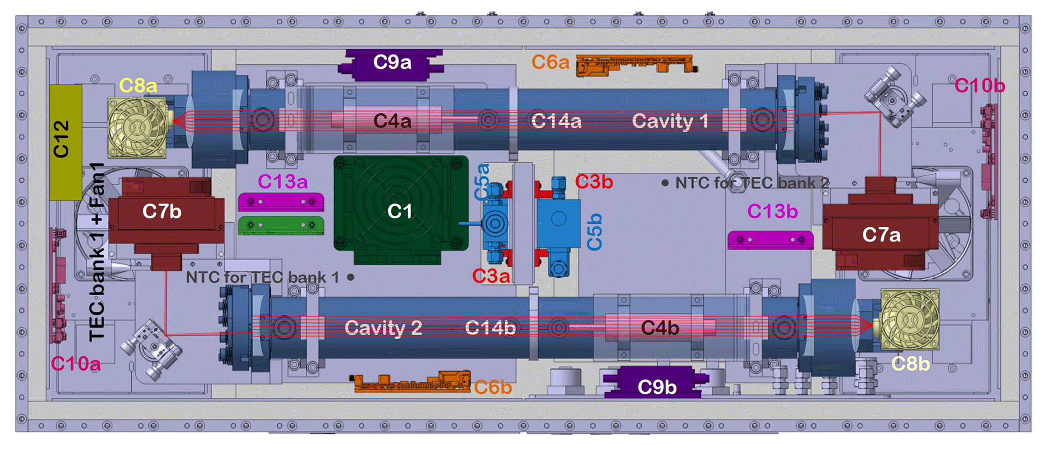
Figure 2 ICOS arrangement inside the AMICA enclosure. Labelled components are described in Table 2. Also shown are optical elements attached to the cavity (high-reflectivity (HR) mirrors and collimating lenses) in light blue and approximations of optical beam paths in red.

Table 2 List of connectors and functional components in AMICA with information on specifications and purpose. Bold face in the fourth column shows components' power source (and output, in case of power converters).

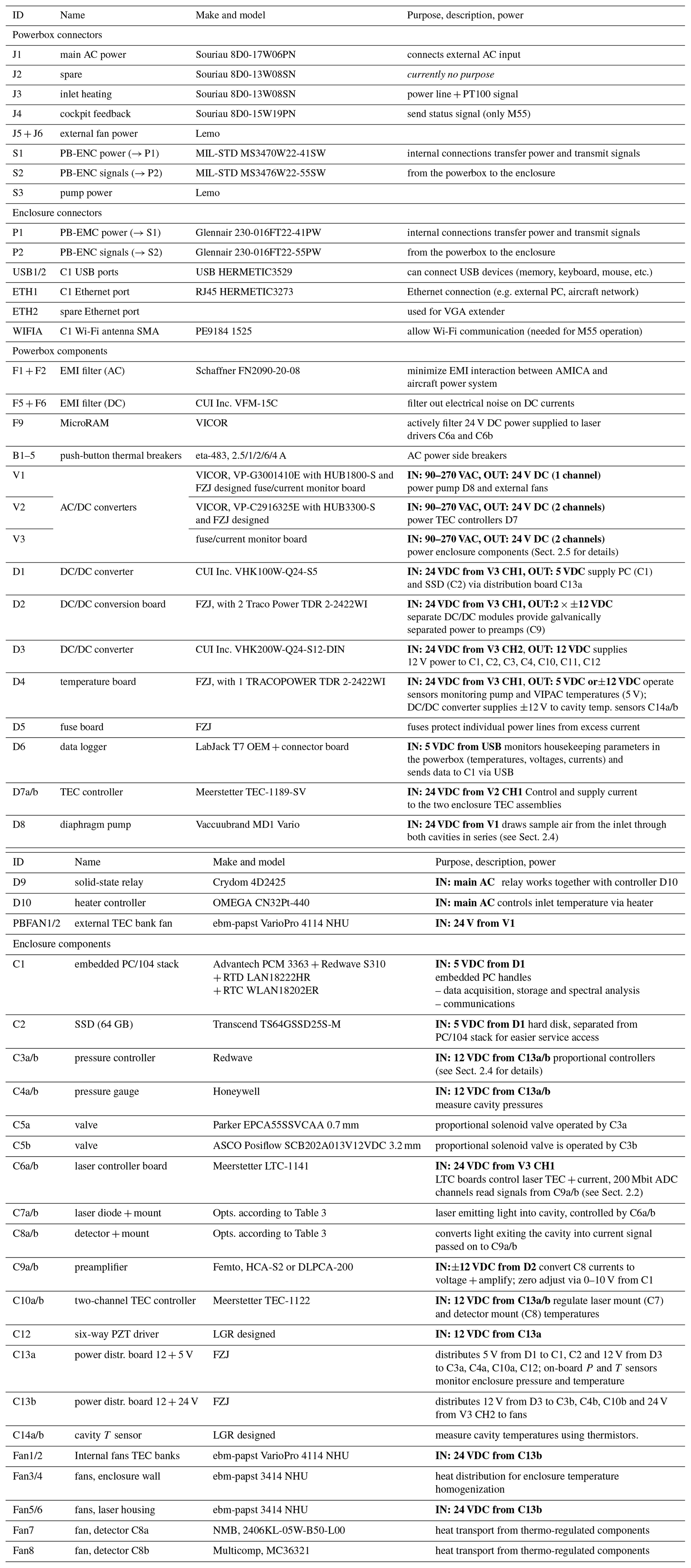
Table 3 Currently implemented ICOS cavity configurations. Each measurement setup consisting of laser and driver board, dielectric mirror, and detector can be used in either one of the two cavity positions in AMICA. Molecules for which sensitivity is too low to measure typical atmospheric mixing ratios in the current setup are shown in italic font.

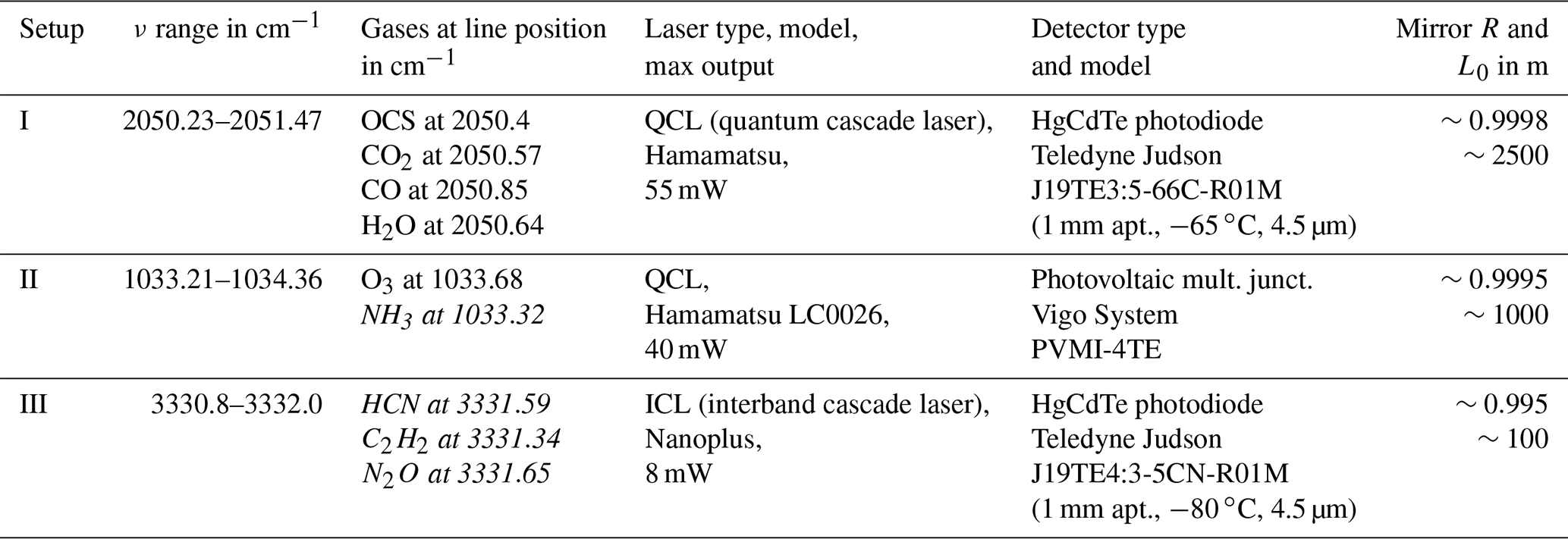
Lasers, mirrors and detectors are exchangeable to tailor the target species to relevant science questions of a particular mission. Specific details on wavelength regions, mirrors, and laser and detector models for the combinations implemented up to now are given in Table 3, and more detailed descriptions are presented together with representative spectra and sensitivity analyses for various trace gases in Sect. 4.

Each laser is operated by a quantum cascade laser (QCL) controller board (C6a/b, in the following referred to as LTC-1141) that offers both thermoelectric control to stabilize the laser temperature and the means to modulate the laser current. In AMICA, the laser current is repetitively ramped over the lasing range or parts thereof to scan over a desired range of typically a few wavenumbers. At the end of each ramp, the laser is turned off to monitor the ring-down decay and the dark signal at the detector (the fitting of dark signal, ring-down time and the measured spectra is described in Sect. 3). Depending on the necessary spectral resolution and on the light attenuation due to trace gas absorption in relation to loss at the mirrors, ramping is done at different rates. Typically, a laser is ramped between 100 and 1000 times per second, the details for each setup are given in Sect. 4.

The detector (C8; typically a photodiode; see Table 3 for specifics of each setup) translates the intensity of light exiting the cavity into a current signal, which is amplified and converted to voltage by a preamplifier (C9) with a nominal bandwidth of 200 kHz. The voltage signal is passed on to a fast analogue to digital converter (AD) channel (sampling rate: 100 MHz, input resistance: 240 Ω) of the corresponding LTC-1141 board (C6a/b). A custom firmware (see LTC-1141 application note under https://www.meerstetter.ch/customer-center/downloads/category/63-application-notes?download=573, last access: 22 July 2021) installed on the LTC-1141 on-board microprocessor averages the signal for N_ramps ramps over a predefined acquisition time t_avg with $N_{\text{ramps}}=t_{\text{avg}}/N_{\text{pts}}$, where N_pts is the number of points per ramp. The averaged signal ramps are transferred to the embedded PC (C1, a PC/104 stack consisting of four modules) via UDP (User Datagram Protocol) data stream (see Sect. 3.1). The data acquisition and processing capabilities of the LTC-1141 (C6a/b) are engaged efficiently in AMICA and significantly reduce computational load on the embedded PC.

2.3 Mechanical design

2.3.1 Design of the thermally insulated ICOS enclosure

As the largest and main compartment, the OA-ICOS enclosure provides the mechanical stability needed for aircraft operation. Its housing and all structural elements are made of aircraft-certified aluminium (EN-AW6061-T651), and the design was laid out in order to withstand forces up to 10 g without plastic deformation. To inhibit corrosion and at the same time retain full electrical conductivity of the housing to minimize electromagnetic interference (EMI, cf. Sect. 2.5), a chromate conversion coating was applied to all parts prior to assembly.

The 12.7 mm thick side panels and bottom plates are bolted together by hexagon socket head cap screws (ISO 4762 – M5×16) tightened to 4 N m into HELICOIL^® thread inserts (M5×1.5D). For additional stability and to reduce shear forces that could weaken the adhesive bonding (see below), stainless-steel pins (Ø5×14, ISO 2338) are driven into pinholes between bolts. Two different enclosure lids were designed: one for cabin operation and one for operation exposed to ambient conditions. The latter one needs to withstand excess pressure of about 1000 hPa inside the enclosure (see below) and consists of a 6.35 mm ($\mathrm{1}/\mathrm{4}$ in.) thick plate with extra enforcement rims where the thickness is doubled to 12.7 mm ($\mathrm{1}/\mathrm{2}$ in.). It is attached by 65 hexagon socket head cap screws (ISO 4762 – M5×16) tightened to 4 N m into HELICOIL^® thread inserts (M5×1.5D) in the enclosure top rim secured with Nord-Lock^® washers (NL5ss). In the lid used for cabin operation, two large openings are cut out and covered with sheet metal attached by eight quick-release fasteners with wing handles (Camloc, D4002 series), allowing for easy and quick maintenance access.

QCLs and photosensitive detectors used in mid-infrared OA-ICOS typically need to be precisely and accurately temperature stabilized, and a good temperature stabilization of the cavities is also beneficial for good long-term precision. To ensure that all individually regulated components can be optimally stabilized with small amplitudes in temperature as well as power fluctuations, the entire enclosure is thermo-regulated to approximately 35 ^∘C by two banks of thermoelectric coolers (TECs) sandwiched between heat sinks equipped with fans on each side (operation and regulation of the TEC assemblies is described in Sect. 2.5). These assemblies were bolted onto the bottom plate using screws (ISO 4762 – M4×16) and each sealed with a flat 4 mm thick EMI shielding gasket (Holland Shielding Systems BC). The enclosure walls were insulated on the inside with polyethylene foam (Ethafoam, 4101 FR Polyethylene Foam, Midland, Michigan, USA; density: 2.2 kg m⁻³, thermal conductivity: 0.06 and 0.05 $\mathrm{W}{\mathrm{m}}^{-\mathrm{1}}{\mathrm{K}}^{-\mathrm{1}}$ at 24 and −5 ^∘C respectively). Additional fans enhance air circulation inside the enclosure to improve temperature uniformity.

For the thermal stabilization to work efficiently and to enable the safe operation when the instrument is placed outside the aircraft cabin and thus exposed to ambient conditions up to 20 km altitude, the enclosure is further designed to be pressure tight. To achieve this, an adhesive with a broad approved temperature range (Polytec Polymere Technologien, EC 101, Waldbronn, Germany) was applied to the joining surfaces of all wall and bottom parts immediately prior to bolting them together. In addition, after assembly, a silicon sealing (Dow Corning 3145) was applied to all inside seams of the enclosure. Inserted into the front plate and sealed with a silicone O-ring is a connector panel with one $\mathrm{1}/\mathrm{2}$ in. bulkhead connector (Swagelok) for the sampling gas stream (see Sect. 2.4), four $\mathrm{1}/\mathrm{4}$ in. bulkhead connectors (Swagelok) for pressure release and flushing of the enclosure, two sealed USB (USB1/2 in Table 2) and RJ45 sockets (ETH1/2), and an SMA-RP (SubMiniature version A reverse polarity) connector (WIFIA) to attach a Wi-Fi antenna (see Sect. 2.5). In the bottom plate, another O-ring-sealed connector panel holds two hermetically sealed connector sockets (P1 and P2) for electrical connection to the powerbox (see below). The pump (D8 in Table 2; cf. Sect. 2.4) is also bolted to the bottom plate, and another $\mathrm{1}/\mathrm{2}$ in. bulkhead connector (Swagelok) is integrated next to it to connect to the pump on the outside and to the end of the sampling gas line on the inside.

2.3.2 Design of the powerbox

Base plate, walls and lid of the powerbox are made of 2.5 mm thick aluminium sheet metal (EN AW 5052 H111). It is mechanically attached to the enclosure at each corner and again near the centre by five M5×125 screws, each supported by a tubular bushing (5.3 mm inner diameter, 10 mm outer diameter, three made of stainless-steel and two of carbon fibre, each with 4 mm wall thickness) to obtain sufficient pre-tensioning. Wiring between the powerbox and the enclosure is done by two connectors, S1 and S2, that attach to the sockets P1 and P2 in the enclosure bottom plate through an opening in the powerbox's lid. Another opening in the lid allows the pump to slide into the volume of the powerbox. Electrical components including AC/DC and DC/DC converters, EMI filters, temperature controllers, and a data logger (all described in Sect. 2.5) are attached either to the bottom or to the sidewalls of the powerbox. Two connectors (J5 + J6) at the sidewalls of the powerbox provide the 24 V power to the external fans of the thermoelectric assemblies mentioned above. On the front of the powerbox, there are two connector panels: one holding the main AC power supply socket (J1) and miniaturized aircraft-style thermal circuit breakers with push-pull on/off manual actuation (B1–B5) and another holding three additional connectors (J2–J4). The purpose and wiring of all connectors are described in Sect. 2.5. The powerbox is not pressure tight, but gaps in the housing are avoided for EMI considerations.

2.3.3 Finite element analysis (FEA) calculations

An FEA model of the AMICA structure loaded with 12 different load cases was run to determine the mechanical strength. All 12 load cases were restarted from the base load case that includes pre-tensioning and embedding of the screws at room temperature. For this base load case, some local plasticity was found after pre-tensioning of the screws in the right-hand side powerbox sheet. The von Mises equivalent stresses are below the yield strength and henceforth below the ultimate strength after embedding of the screws.

Six operative load cases at flight level with accelerations set at ±4 g in both flight direction and horizontal transversal to the flight direction and ±7 g in vertical transversal to the flight direction were analysed in conjunction with an ambient temperature of −60 ^∘C and an internal excess pressure of 1000 hPa in the enclosure. At these expected operative loads, repeated occurrence of plasticity in parts should be avoided as much as possible to prevent a low-cycle fatigue failure, and the results indicate that this is fulfilled. No additional local plasticity was found for the operative load cases in the right-hand side powerbox sheet, but some local plasticity was found in the top powerbox sheet. The von Mises equivalent stresses are below or at the yield strength at these locations but far away from the ultimate strength. Existing plasticity will not increase further in a successive flight.

Six emergency load cases with accelerations set at 10 g in all directions were chosen to simulate two situations. The first is the transport of AMICA through airfreight, while the second concerns acceleration specifications given by the operators of the carrier aeroplanes and valid for emergency landing conditions. Since both situations have the same environmental conditions with respect to ambient temperature and internal excess pressure, they are considered one situation. The accelerations applied are valid for airfreight with a safety margin of +10 % and encompass the accelerations occurring at emergency landing conditions. At this special load level, plasticity in parts is allowed, but failure leading to disintegration of parts is prohibited. Some additional local plasticity was found for the emergency load cases in the right-hand side powerbox sheet and at one of the bore holes of the rear grey frame plate. The von Mises equivalent stresses are slightly below or above the yield strength at these locations but far away from the ultimate strength.

2.3.4 Aircraft-specific mounting considerations

For HALO operation, AMICA is mounted in a standard rack (R-G550SM, EPA-DLR-00004-000) using a set of adapters (for details, see Fig. S1). It conforms to all requirements with respect to total weight and position of the centre of gravity; thus, the mechanical airworthiness certification is inherited from that of the rack. Because the rack is mounted inside the cabin with a set of pre-installed shock absorbers, no additional vibrational isolation hardware is used.

On M55 Geophysica, AMICA is installed inside a dome on top of the aircraft. Specific mounting plates have been designed to attach AMICA onto the base frame of the dome (see Fig. S2), including four springs (Enidine WR12-300-08) with the following characteristics: in normal direction a maximum force per spring of 4.65 kN, resulting in a spring deflection of 37.1 mm and in both shear directions a maximum force per spring of 5.55 kN, resulting in a spring deflection of 39.1 mm. The springs are designed to withstand the normal and shear forces that occur due to the different load cases. For the operative and emergency landing load cases, the springs will stay elastic. For airfreight emergency loading and then only if the stowage of AMICA occurs perpendicular to the prescribed flight direction, the two front springs will exceed their elastic bearing capacity and will hit the internal limit stop. Another purpose of the springs is to decouple the instrument from the aircraft body movements, mainly to absorb potentially heavy shocks during take-off and landing. The effectiveness of the springs was tested during the first deployment using two vibration sensors (SlamSticks, Mide Technology LOG000200-0006, Medford, Massachusetts, USA) attached to each side of one spring. The vibrational data of several hours was cut in time sequences of 30 s of data each. Then from every time sequence a fast Fourier transform (FFT, in the range from 0 to 1000 Hz) and subsequently a power spectral density (PSD) and a cumulative power spectral density (CPSD) were made to obtain the root-mean-square (rms) values of the directional accelerations (g_rms), both for the data on the M55 side and on the AMICA side of the springs. The attenuation of the vibrations was then calculated from the ratio of the g_rms values. Depending on the direction, the attenuation lies between −18 dB for the flight direction and −25 dB for both directions perpendicular to the flight direction (for more detail, see Fig. S3).

For mounting, AMICA is lifted onto the aircraft by crane and the exact position is adjusted by hand. For this purpose, four shackles and hand bars are attached to the enclosure at the four corners (also included in Fig. S2).

Because AMICA is mounted to the M55 Geophysica as a unique entity, mechanical stability had to be certified and documented. In its Geophysica setup, AMICA is laid out for elastic deformation up to 7 g with fully preserved functionality and plastic deformation up to 10 g. This was simulated in the FEA calculations described above. In addition, a shaker test with a dummy of the AMICA housing internally equipped with dummy weights closely resembling the distribution of the electronics and ICOS hardware was carried out (at MOOG CSA Engineering, Mountain View, California) according to the test procedure RTCA/DO-160G (elastic deformation for 7 g acceleration in X, Y and Z direction) and successfully passed. It confirmed that the AMICA housing responded to a 0.5 g sine sweep before and after the application of random vibrations with no significant difference in system behaviour.

2.4 Sampling and flow system

The sampling system has been designed to ensure rapid transfer from the inlet to (and through) the cavities (effective instrument time resolution is ultimately limited by the cavity flush time) and to keep pressure inside each cavity constant to warrant straightforward analysis of the ICOS spectra with good precision. Cavity pressure P_cav is chosen as a compromise between absolute sensitivity (pressure correlates with number density and therefore absorption of each species) and spectral resolution (which deteriorates at higher pressure as a result of pressure broadening). Depending on the expected mixing ratios of the measured species and the wavelength separation of their absorption peaks, pressures employed in ICOS systems typically range from a few hectopascals (hPa) to about 200 hPa. Because AMICA is operated on aircraft, the lowest possible cavity pressure is further limited by the ambient pressure at the sampling inlet.

2.4.1 General setup

A schematic of the AMICA sampling and flow system is shown in Fig. 3. Sampling air enters the system at a $\mathrm{1}/\mathrm{2}$ in. bulkhead connector port (Swagelok) in the enclosure wall, equipped on the outside with a 7 µm filter (Swagelok SS-4FW7-7) coated with Sulfinert^® (SilcoTek GmbH, Bad Homburg, Germany) to prevent dust from entering the system. Inside the enclosure, the air flows through a system of tubing (Sulfinert^®-treated $\mathrm{3}/\mathrm{8}$ and $\mathrm{1}/\mathrm{4}$ in. stainless-steel tubing), valves (C5, see below) and the two cavities in series. A second Sulfinert^®-treated filter with 2 µm pore size (Swagelok SS-4FW4-2) is placed directly upstream of the first cavity to prevent small particles that have passed through the first filter or released from the valve seals to enter the cavities and contaminate or damage the mirrors. The two 508 mm long cavities each have a volume V_cav of 0.911 L and are coupled in series.

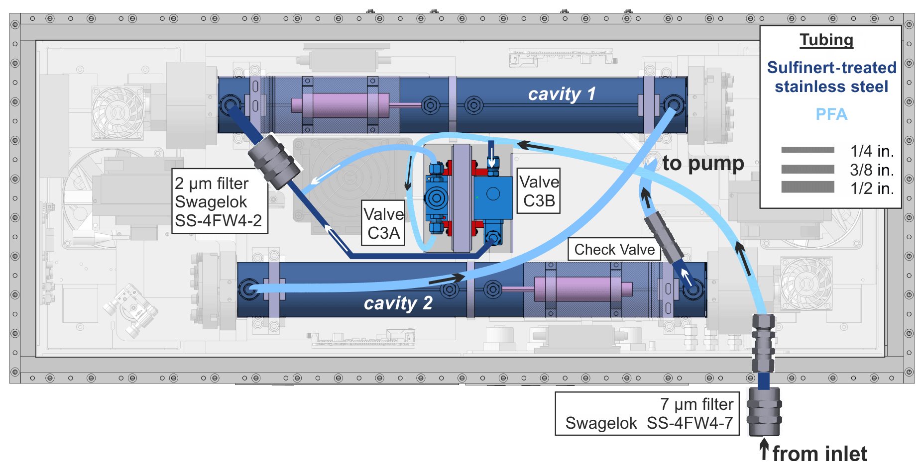
Figure 3 Sample gas flow system inside AMICA. The T-junctions where the gas flow branches off to or from the two valves C3a and C3b are marked by yellow circles.

The sampling air is drawn into and through the entire system at flow rates F between 0.8 SLM (standard litre per minute) (with P_cav≈45 hPa) and 1.6 SLM (with P_cav∼80 hPa) by a pump (D8) placed downstream of the second cavity and a check valve to avoid backflow into the system. The pump exhaust blows air directly into the powerbox for extra ventilation therein. The Vaccuubrand MD1 Vario pump was selected as a compromise between weight, power draw, internal heat generation and flow rates at typical AMICA cavity pressures.

2.4.2 Pressure regulation

Because the ambient pressure can range from ∼1000 hPa at ground level down to about 55 hPa at the highest flight altitudes of 20 km, a system of two parallel proportional solenoid valves with orifices of 0.762 mm (C5a) and 3.2 mm (C5b) is used to precisely regulate cavity pressure P_cav. The valves are controlled by separate pressure controllers (C3a/b) with the set point of controller C3a being ∼1 hPa smaller than that of controller C3b. There is a pressure gauge (C4) at each cavity, but only the reading from gauge C4a at cavity 1 is wired to the controllers (C3a/b) for pressure regulation. The pressure gauges (C4) are factory calibrated with an accuracy of 0.1 %. Recalibration before and after field campaigns is done in our laboratory against an absolute pressure Baratron (MKS). Note that cavity temperature is measured with a thermistor that is calibrated in a glycol bath and accurate to about 50 mK.

Pressure regulation and response of P_cav to ambient pressure have been tested in the laboratory by pumping down a 50 L bottle through the original AMICA inlet tubing used in HALO (cf. below) with two additional pressure gauges placed at the bottle (Fig. 4). At ambient pressures above ∼200 hPa, cavity 1 pressure is typically regulated to ±0.2 hPa (1σ standard deviation) around the higher set point, with the larger valve remaining fully closed because the lower set point is not reached. When ambient pressure drops below ∼200 hPa, the resistance of the smaller valve C5a becomes too large even when fully opened, and the cavity pressure starts to drop below the set point of the corresponding regulator C3a. When this happens, the second regulator C3b with the slightly lower set point starts to open the larger valve C5b, which allows for pressure regulation to ±0.6 hPa (1σ standard deviation) down to an ambient pressure about 10 hPa larger than the lower set point. When ambient pressure drops further, both valves remain fully open, and the cavity pressure drops and varies with ambient pressure at a few hectopascals below it. As a consequence of the additional flow resistance of the tubing between the cavities, the pressure inside the second cavity is approximately 1.5 hPa lower than the cavity 1 pressure.

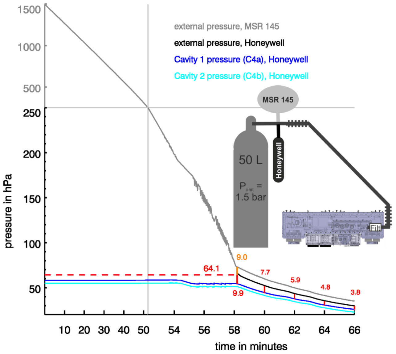
Figure 4 Experimental determination of AMICA cavity pressures (dark blue: cavity 1; light blue: cavity 2) to simulated ambient pressure at a 50 L gas bottle measured by the pressure gauge of an MSR 145 data logger (grey, absolute range 0–2000 hPa, certified accuracy of ±2.5 hPa between 750 and 1100 hPa) and a Honeywell gauge identical to the gauges C4 inside AMICA (black, range 0–69 hPa). At 64.1 hPa, the offset between the two gauges is 9.0 hPa (shown in orange); at pressures within the range of the Honeywell gauge, we deem this sensor more accurate than the MSR 145 and more comparable to the C4 gauges inside AMICA. For the regime where cavity pressure cannot be regulated, differences between simulated ambient pressure at the 50 L bottle and cavity 1 pressure (measured by gauge C4a) are shown in red. Note that the scaling of the x and y axes changes at 52 min and 250 hPa respectively as shown by the light grey lines.

The observed pressure fluctuations (given as 1σ standard deviations of pressure recorded at 0.5 Hz) most likely result from the response of the regulating valves. This is supported by the observations of higher fluctuations of the order of 2–3 hPa in preliminary tests using the larger valve at ∼1000 hPa ambient pressure and reduced fluctuations at pressures below the lower set point when both valves remain fully open.

2.4.3 Aircraft-specific inlets

During aircraft operation, sampling air is taken in through a primary intake sticking out of the aircraft boundary layer, and it then needs to be transferred to the instrument inlet. For AMICA, this has so far been implemented for the in-cabin operation on the German HALO, and for the operation in a dome on top of the high-altitude aircraft M55 Geophysica. Both inlet systems are rear facing to avoid the intake of liquid water, ice and large aerosol particles (McQuaid et al., 2013). They are briefly described and characterized here.

On HALO, a rear-facing 0.5 in. stainless-steel tube in a standard Trace Gas Inlet (TGI; see https://www.halo.dlr.de/instrumentation/inlets/inlets.html#TGI, last access: 4 May 2021) near the front of the aircraft is used as primary inlet. The diameter is reduced to $\mathrm{3}/\mathrm{8}$ in. at the inlet, and the air is transferred to the filter right in front of the AMICA instrument inlet via a 214 cm long $\mathrm{1}/\mathrm{4}$ in. inner diameter Sulfinert^®-coated (SilcoTek, Bellefonte, Pennsylvania, USA) stainless-steel tube with a 10 cm Sulfinert^®-coated bellow on each side to avoid stress on the connectors. The primary inlet is not actively heated at the tube used for AMICA, but heat transfer from a neighbouring inlet tube ensures it is warmer than ambient temperature. The transfer tube inside the cabin is not heated or insulated.

A dedicated shared primary inlet with three separate rear-facing tubes for AMICA and two other instruments was developed for the dome on top of the M55 Geophysica (an illustrated photo is given in Fig. S4). The AMICA tube is a 40 cm long $\mathrm{3}/\mathrm{8}$ in. Sulfinert^®-coated stainless-steel tube. A 200 cm long $\mathrm{1}/\mathrm{4}$ in. inner diameter Sulfinert^®-coated stainless-steel tube transfers the air from the primary inlet to the instrument. As described above for HALO, two bellows are placed at each side of the transfer tube to avoid stress and breakage.

The time lag for the sampling air to flow from the inlet outside the aircraft to cavity 1 is approximately 6 s at ground level and 0.6 s at an ambient pressure of 100 hPa, corresponding to a distance of 120 m at an aircraft speed of 200 m s⁻¹. The additional time lag for the second cavity is 2.8 s (equivalent to 560 m at an aircraft speed of 200 m s⁻¹). The flush time for each cavity (given by $V_{\text{cav}}\cdot [P_{\text{cav}}/\mathrm{1013}\mathrm{hPa}]\cdot [\mathrm{273}\mathrm{K}/T_{\text{cav}}]/F)$ is about 2.5 s, which sets a limit to the actually useful time resolution of the measurement to 0.4 Hz (equivalent to 500 m distance at an aircraft speed of 200 m s⁻¹).

2.5 Power concept and electronic design

2.5.1 AC power supply

A complete block diagram of the powerbox is shown in Fig. 5. AMICA is powered only by a single-phase AC power supply line through connector J1 at the powerbox connector panel. Inside the powerbox, the AC current is passed through two filter modules (F1 and F2) to minimize conducted EMI interaction between AMICA and the aircraft power system. It is then distributed to supply power to four component groups: (i) an inlet heating, (ii) pump and fans, (iii) enclosure temperature control system, and (iv) ICOS measurement system. Prior to flowing in any components or power converters, the current is passed through thermal circuit breakers (B1–B5) to protect the system from currents exceeding their nominal values (e.g. due to component malfunctions or unforeseen short circuits). The breakers B1, B3, B4 and B5 are chosen with current limits of 2.5, 2, 6 and 4 A for component groups (i) to (iv) respectively, reflecting their expected maximum power consumption during nominal operation. Additionally, the breakers allow for push-pull manual actuation to switch on/off power to individual component groups separately for test and diagnostic purposes.

Figure 5 Simplified block diagram of the AMICA powerbox. Component and connector positions and sizes are not drawn to scale; identifiers correspond to those used in Table 2. Custom-designed boards are shown in green. Power wires are shown as thicker black lines labelled with voltage and nominal current, with dark red boxes showing the position of ferrite beads. Thinner lines mark signal connections for various sensors.

2.5.2 Inlet heating

Inlet heater elements (i) are directly powered by the AC current. A temperature controller (D10) in combination with a relay (D9) allows for adjusting the inlet temperature to a set point (set in the D10 menu). Power to the inlet and a PT100 temperature probe for control are wired through connector J3. Inlet heating has been used with a set point of 30 ^∘C during M55 Geophysica deployment but was disabled during operation in the HALO cabin.

2.5.3 AC/DC conversion

All other components in AMICA require DC power. This is generated by AC/DC converter modules V1–V3. These converters from Vicorpower have an auto-ranging AC input that automatically senses the AC supply voltage between 90 and 132 V, as well as 180 and 264 V, and the frequency over a range of 47–440 Hz, so AMICA can be operated inside a laboratory (115 or 230 V at 50 or 60 Hz) and inside aircraft (typically 115 V at 400 Hz) without any internal modifications. The outputs of V1–V3 are 24 V DC each. Self-made add-on boards are installed directly onto the output terminals of V1–V3 to sense the currents for monitoring by using special Hall ICs (integrated circuits). The boards also detect the output voltage and distribute the output power into several current-limiting paths by using small SMD (surface-mounted device) fuses specially designed for space-limited circuit boards (“nano fuses”, Littelfuse, Chicago, USA).

2.5.4 Pump

V1 powers the pump D8 through connector S3 and the two fans attached externally to the TEC assemblies through connectors J5 and J6. Pump and fan power lines are fused at 6 and 0.5 A each respectively.

2.5.5 Temperature regulation of the enclosure

The TEC assemblies themselves are independently run by two TEC controllers (D7a/b) powered by the two V2 output channels, each fused at 10 A. Each TEC assembly consists of 16 Peltier elements (30×30 mm²). Both sign and magnitude of voltage and current are modulated by the TEC controllers (D7a/b) in order to stabilize the measured temperature as near as possible to the 35 ^∘C set point (set in the D7 menu via PC interface using a Mini USB service port). The negative temperature coefficient thermistor (NTC, 1 MΩ) temperature probes are placed inside the enclosure at some distance from the TEC assemblies but each closer to the TEC assembly connected to the same controller as the probe (exact positions are shown in Fig. 2). Cables for power wires and temperature probes are run from the controllers into the enclosure via the S2/P2 connection.

2.5.6 Power supply to ICOS components

All components of the actual ICOS measurement system are powered by V3 through two output channels fused at 10 A each. Channel 1 provides power to powerbox temperature board D4; the laser controllers C6; and components C3, C4, C10, and C12 that operate at 12 VDC. The 24 VDC supplying the laser controllers C6a/b is passed through a MicroRAM (F9) for EMI filtering and subsequently fused at 4 A before being passed through connection S1/P1 directly to the LTC-1141 boards C6a and C6b, which handle powering of the respective lasers and their TECs. A parallel line from V3 channel 1 is passed through EMI filter F6, from which separate lines lead to temperature board D4 and DC/DC converter D3. D4 provides 5 VDC power to temperature sensors inside the powerbox (see Housekeeping section below) and ±12 V to the cavity temperature sensors in the enclosure through connection S2/P2. D3 provides 12 VDC, and two output lines, each fused at 6.3 A, pass the voltage via the S1/P1 connection to two distribution boards inside the enclosure that supply the 12 VDC components in their vicinity (see Table 2 for the detailed allocation). V3 channel 2 is first passed though EMI filter F5 and then divided into three supply lines. One of these, fused at 4 A, transfers 24 VDC directly through S1/P1 to distribution board C13b, from which all fans (listed in Table 2) in the ICOS enclosure receive their power. The second filtered line from V3 channel 2 is converted to 5 VDC in D1, fused at 10 A and passed through S1/P1 to distribution board C13a. The 5 VDC powers the embedded PC (C1) and SSD (C2) as well as two sensors placed on C13a that monitor temperature (Texas Instruments, LMT86) and pressure (Infineon, KP215F1701) inside the ICOS enclosure. The third filtered V3 channel 2 line is used as input for DC/DC conversion board D2 to generate two independent ±12 VDC sources with particularly low ripple output to provide up to 0.5 A to the two highly sensitive preamplifiers C9a and C9b through the S1/P1 connection.

2.5.7 Grounding

The AMICA grounding concept distinguishes between three grounding systems: earth ground (chassis ground), supply grounds, and analogue/digital grounds.

Earth ground plays a special role as AMICA operates on high AC voltage (100 to 250 VAC at up to 12 A). Due to the two EMI filters F1 and F2, which utilize Y capacitors between the live and neutral conductor, leakage current occurs and flows from the live conductor to the filter casings, which are connected to the powerbox metallic housing, and flows back to the power source. This leakage current may flow through other paths (such as a human body touching the instrument) and can cause electric shock if the ground is inefficient or interrupted. As the entire AMICA housing (ICOS enclosure and powerbox) is electrically conductive, the whole chassis becomes an earth ground and must be grounded to the power source properly. To ensure that AMICA is always well grounded to system power during laboratory operation, the dedicated grounding threaded rod at the powerbox front panel has to be connected to the ground using an earthing strap. For operation on aircraft, additional grounding interfaces are placed at the four corners of the enclosure. Internal electric components benefit from the instrument housing's good EMI characteristics as it keeps out external disturbances of any kind and vice versa.

Inside the instrument, supply grounds and analogue/digital grounds are managed to connect to ground according to the internal assemblies and structures of the instrument with the goal of reducing problematic internal EMI and minimizing noise coupling between components. Interconnections are laid out to avoid potential internal ground loops wherever possible. The other measure is to provide electrical components or component groups with independent and isolated power sources. This is done for example by the DC/DC conversion board (D2) to supply the two high-sensitivity preamplifiers C9a/b without ground loops.

2.5.8 Housekeeping

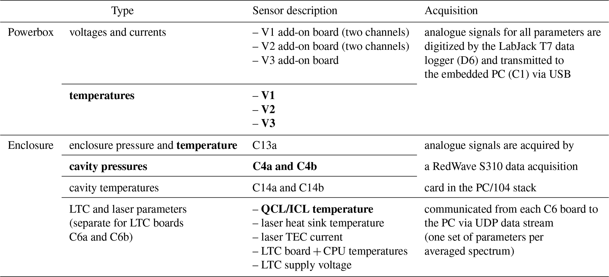
As mentioned above, voltages and currents of each AC/DC converter output channel are monitored by using self-made PCBs (printed circuit boards) as add-on boards for V1–V3. For each voltage monitor, a high-precision DC voltage isolation sensor (ACPL-C87AT, Broadcom) is used that utilizes optical coupling technology with a fully differential amplifier to provide an isolated analogue output signal. Current sensor ICs (ACPL-C87AT, Allegro MicroSystems) each use an integrated Hall transducer to measure the magnetic field of the applied current flow and convert it proportionally into an isolated voltage. These components were chosen following the grounding concept to reduce the signal ground loops. Temperatures of the three AC/DC converter boards and the pump are monitored using integrated circuit temperature sensors (Texas Instruments, LMT86) powered and read from temperature board D4.

Voltage, current and temperature signals are digitized by a LabJack T7 data logger powered from the embedded PC (C1) via a USB line passed through connection S2/P2. Through the same USB line, the set of 14 parameters is regularly read by the software on the embedded PC. The monitoring of these parameters is needed to observe smooth operation of each component in the power supply system, and the data can help in case trouble-shooting becomes necessary.

In the enclosure, signals from the temperature and pressure sensors on the C13a board and from the temperature probes C14 and pressure gauges C4 of the two cavities are acquired by the embedded PC from analogue input channels of a data acquisition card (RedWave S310) in the embedded PC/104 stack. Parameters related to the lasers C7 (laser and heat sink temperatures) and their driver boards C6 (voltage, board and processor temperature) are communicated via UDP data stream together with the spectra from the C6 boards (see Communications section below and Sect. 3.1).

2.5.9 Communications

AMICA contains a self-contained and fully operational embedded PC (C1; note that a previous version of AMICA contained two independent embedded PC/104 stacks, cf. Sect. 5) equipped with a 64 GB SATA SSD (C2) and running under a Linux operating system (Lubuntu 18.04). Communications ports are wired to appropriate connectors at the enclosure connector panel (details given in Table 2). Two USB ports (USB1/2) allow for connection of computer peripherals such as keyboard and mouse as well as the use of USB memory devices. An RJ45 connector (ETH1) allows for LAN connections to an external PC or network via the embedded PC's 1 Gbit Ethernet port. However, cable-based LAN connections are not always feasible, e.g. on the M55 Geophysica when the dome cowling is closed and the instrument cannot be accessed. To still be able to communicate with AMICA, a wireless LAN module (RTD, WLAN18202ER) in the PC/104 stack is wired to an SMA connector (WIFIA) in the enclosure connector panel with a Wi-Fi antenna attached on the outside. With this setup, Wi-Fi connections between AMICA and a laptop or desktop PC are possible up to about 200 m distance. Another RJ45 connector (ETH2) is used for VGA extension via RJ45 cable that allows for the connection of an external screen to the PC's VGA port even when the enclosure is fully closed. This can be useful to directly work on the AMICA PC in the laboratory, or for troubleshooting if an external Ethernet connection can not be established.

A PC/104 module with two additional Gbit Ethernet channels (RTD, LAN18222HR) is used for internal communication between the embedded PC (C1) and the LTC-1141l boards (C6a/b). A TCP/IP protocol is used for initialization of the boards at software start-up and for sending commands (e.g. to change the temperature set point) to or receiving status information from C6a and C6b. A data stream consisting of the acquired and averaged spectra as well as some additional parameters (cf. Sect. 3.1) is transferred one-way from each LTC-1141 to the PC via UDP data stream.

2.5.10 EMC test

To certify proof of airworthiness, an electromagnetic compatibility (EMC) test was carried out according to the environmental conditions and test procedures for airborne equipment (RTC-DO160 E, category M; testing was done at steep GmbH, EMC Service, Bonn, Germany). AMICA passed the test procedure without exceeding any of the given thresholds.

3 Data acquisition and analysis

Instrument control and data acquisition are handled by a software package written in Python 3.7.6 that runs under a Linux environment (Lubuntu 18.04) on the PC/104 stack in the pressurized enclosure. Below, we briefly describe the implementation of data acquisition and storage and the algorithms used to analyse the ICOS spectra and retrieve trace gas mixing ratios.

Table 4 List of housekeeping parameters routinely monitored during AMICA operation. Parameters marked by bold face are sent to the HALO web user interface PLANET (ATMOSPHERE, Wessling, Germany) for real-time online monitoring.

3.1 Data acquisition

In the current version, the AMICA software uses one continuously running data acquisition loop to consecutively read spectra and housekeeping data (a complete list of monitored parameters is given in Table 4):

• Time averaged ICOS spectra from each LTC. At each time interval t_int, the LTC sends an ICOS spectrum averaged from N_ramps (cf. Sect. 2.2) together with six parameters related to laser and LTC status (see Table 4 for details) to the PC via UDP stream in packages of 256 floating-point numbers each. The packages are read by a socket command inside a loop that puts the housekeeping parameters into corresponding named variables and the spectra into a netCDF type structure, which is synchronized to the SSD hard disk every 60th data acquisition cycle.

• Cavity and enclosure pressures and temperatures. Both pressure and temperature sensors in the enclosure and in each cavity are sensed as analogue voltages and converted to digital numbers by the RedWave S310 data acquisition card in the PC/104 stack. The six parameters (listed in Table 4) are read into named variables in the AMICA software via the S310 application programming interface (API).

• Powerbox temperatures, voltages and currents. The AMICA software calls the LabJack T7 (C6) to transfer the readings on the 14 AD channels (given in Table 4) via USB connection. Actual temperatures, voltages and currents are calculated from the received voltage signals and stored in named variables.

At the end of each data acquisition cycle, all housekeeping parameters listed in Table 4 are converted into a single string and added to an ASCII file on the SSD. During HALO flight missions, a selection of these data (marked in Table 4) is additionally sent to the aircraft server as a UDP stream. An interactive software version for laboratory use during tests and calibrations displays all housekeeping data in a widget displayed on the screen (a screenshot of this widget is given in Fig. S5).

3.2 Analysis of ICOS spectra

Three different sections are extracted from the averaged ramps (illustrated in Fig. 6) and analysed. First, the points between the start and the laser turn on (grey region in Fig. 6) are averaged to calculate the detector dark signal S_dark. Second, an exponential decay is fitted to points (the broad region where this fit is made is marked red in Fig. 6) between the laser turn-off and the point when the signal has decayed back to S_dark+3σ(S_dark) to deduce the ring-down time τ (using the method of linearly fitting the time shifted signal given in Sayres et al., 2009). To avoid contribution to the fit of the actual decay time of the laser output and the time for the laser light to be coupled into the cavity, points within approximately 2τ after laser turn-off are excluded from the fit. Because the background τ of an empty cavity is needed to determine mirror reflectivity R and the mean absorption free path length L₀, it is important that the laser ramp ends in a spectral region without any absorption by trace gases present in the atmosphere. From the fitted τ, $L_{\mathrm{0}}=c\cdot \mathit{\tau }$ and $R=(\mathrm{1}-L_{\text{cav}}/L_{\mathrm{0}})$ are calculated with the speed of light $c=\mathrm{2.998}\times {\mathrm{10}}^{\mathrm{8}}$ m s⁻¹ and cavity length L_cav=508 mm.

Figure 6 (a) QCL current (dashed line, right axis; the 268–360 mA ramp is slightly curved to arrive at the linear wavenumber scale indicated on the top x axis) and detector voltage signal past the preamplifier (solid black line, left axis; ramps averaged over 30 s) for AMICA cavity 1 in the 2050 cm⁻¹ setup. Three periods are marked by the coloured areas – (i) grey: only detector dark signal (with zero offset) is observed; (ii) blue: period used for spectral analysis; (iii) red: period after the QCL stops emitting, when the signal decays exponentially due to “ring down” of the light in the cavity. A ring-down fit is shown by the red line. For the spectral fitting region, a measured baseline spectrum with no absorbers present (purple) and a fitted spectrum (blue) are also shown. (b) Measured and fitted spectra from (a) shown in absorption space. (c) Difference between the fit and the measured spectrum (fitted–measured). Panels (b, c) only show data for the region that is actually fitted, i.e. the blue shaded region in (a). Absorption line positions coloured according to different gases are indicated in all panels by vertical lines for better comparison.

Third, the part of the active laser ramp (blue region in Fig. 6) is extracted over which spectral fitting is employed to deduce trace gas mixing ratios. Prior to spectral fitting, the points/time along the ramp have to be converted to a wavenumber scale. For each laser source, an etalon fit was experimentally determined when the temperature and ramp current settings were initially tuned to the desired wavenumber range. In Eq. (1), the wavenumber is expressed as a function of laser current:

$$\begin{array}{}\text{(1)}& \begin{array}{rl}\mathit{\nu }\left(I_{\text{laser}}\right)=& {\mathit{\nu }}_{\mathrm{0}}+\mathrm{1.0}\times {\mathrm{10}}^{\mathrm{9}}[a_{\mathrm{1}}+a_{\mathrm{2}}\cdot I_{\text{laser}}\\ & +a_{\mathrm{3}}\cdot I_{\text{laser}}/{\log }_e\left(I_{\text{laser}}\right)\\ & +a_{\mathrm{4}}\cdot {\log }_e\left(I_{\text{laser}}\right)/I_{\text{laser}}\\ & +a_{\mathrm{5}}/I_{\text{laser}}]/c.\end{array}\end{array}$$

Here, ν₀ is a fixed wavenumber within the spectrum (typically chosen at or in relation to prominent absorption peak within the spectral range) and the bracketed part is the shift in gigahertz (GHz) from this peak with fitting parameters a₁–a₅, determined using an etalon. For this equation to work, the ν₀ point in the spectrum needs to remain in the same position in terms of I_laser, which is usually the case after temperatures of the laser and the laser housing have stabilized. Small drifts are actively adjusted by the software adding an offset (<0.1 K) to the temperature set in the LTC, and the wavenumber to I_laser relation given by Eq. (1) holds with the same fitting parameters when this is done. This is regularly checked and validated by testing if all peaks appear in the correct positions when measuring standards with many absorption peaks present in the spectral range. Using a relation with respect to I_laser rather than points or time along the ramp in Eq. (1) allows for the possibility of applying a curved ramp of I_laser resulting in a quasi-linear wavenumber scale that makes spectral fitting easier.

Spectral fitting following the method described by Sayres et al. (2009) has been implemented in Interactive Data Language (IDL) code and has been used to process the spectra recorded during the M55 Geophysica field campaigns described in Sect. 5.1 and 5.2 (note that proprietary ABB–Los Gatos Research software was used for instrument control and spectra acquisition during these campaigns, with two separate PCs handling the two ICOS channels). Encoding of the full spectral fitting algorithm in Python is currently in progress and shall not only be used for post-processing of recorded spectra but also for real-time processing during measurement flights. In the current Python software actually running on the AMICA instrument, a less computationally demanding approach is used to fit trace gas concentrations: using an experimentally measured baseline (with the cavity filled with Argon at 99.9999 % purity), the spectrum is transformed into absorption space and a Lambert–Beer fit of wavelength-dependent absorption A(λ) is solved for the concentrations c_i of different absorbers with

$$\begin{array}{}\text{(2)}& {\displaystyle }{\displaystyle }A\left(\mathit{\lambda }\right)=L_{\mathrm{0}}\sum _i{c}_i{\mathit{\alpha }}_i\left(\mathit{\lambda }\right),\end{array}$$

where α_i(λ) is the wavelength-dependent absorption coefficient for each absorber based on the line parameters from the HITRAN2012 database (Rothman et al., 2013). This method is only an approximation as it does not take into account the cavity broadening effects (cf. Sayres et al., 2009), which are small as long as

$$\begin{array}{}\text{(3)}& {\displaystyle }{L}_{\text{cav}}{c}_i{\mathit{\alpha }}_i\left(\mathit{\lambda }\right)\ll \mathrm{1}-R.\end{array}$$

When this condition is not met, the effective path length L_eff is reduced compared to L₀ determined for the empty cavity and the sensitivity is reduced and the analysis is complicated, because the variation of L_eff with wavelength over a broadened absorption peak leads to additional broadening in the observed spectrum compared to the Voigt profile calculated from the broadening coefficients in HITRAN. The simplified fitting method in absorption space has been used for the spectra recorded during SouthTRAC (Sect. 5.1) and for the calibration experiments (Sect. 4).

In theory, these spectral fitting procedures avoid the need for frequent calibrations and in particular an in-flight calibration system that would substantially add to the instrument dimensions and weight, complicate airworthiness and safety compliance certification, and lead to data gaps during calibration periods. There are, however, some caveats to this “calibration free” fitting:

• While absorption line parameters are constant by definition, they still need to be accurately known, and stated line uncertainties in HITRAN vary significantly.

• The absorption path length determination from the ring-down fit needs to be precise and accurate.

• Precise line locking must ensure that the scanned wavelength scale is constant.

• The baseline must remain stable or at least well characterized by a mathematical function that can be fully included in the spectral fit.

• Cavity temperature and pressure need to be accurately known and constant over the timescale of the measurement.

While the last point is addressed by regular tests and, if needed, recalibration of the cavity pressure and temperature sensors (see Sect. 2.4), the other points are issues specific to setup or absorption line and are discussed for each setup in Sect. 4. Clearly, for operational channels producing atmospheric data to be used for scientific purposes, validation of the complete system to detect potential systematic errors and to ensure data quality is done in the laboratory at regular intervals by measuring “zero air” as well as known standards. Some results of these experiments and a discussion of issues detected is given in Sect. 4.

4 Characterization of implemented ICOS measurement setups: spectra and calibrations

In this section, different laser, mirror and detector setups to measure specific target gases are described and characterized. An overview of these setups is given in Table 2; detailed descriptions are given in the subsections below. Besides these, a wide variety of setups is theoretically possible, targeting many trace gases.

4.1 OCS, CO₂, CO and H₂O at 2050–2051 cm⁻¹

A quantum cascade laser (QCL, Hamamatsu), operated at 18.6 ^∘C and ramped over the current range 268–360 mA, emits light over the wavenumber range of 2050.23–2051.47 cm⁻¹. In this spectral window, OCS (major absorption lines at 2050.39 and 2050.86 cm⁻¹), CO (major absorption line at 2050.80 cm⁻¹), CO₂ (major absorption line at 2050.60 cm⁻¹) and H₂O (major absorption line at 2050.63 cm⁻¹) can be measured. Several O₃ absorption lines also exist in this window, but absorption at typical cavity pressures is completely negligible even at stratospheric ozone levels in the parts per million (ppm) range.

A set of typical spectra in both intensity and absorption domains for this setup is shown in Fig. 6. Absorption peaks for CO₂, H₂O and OCS are spectrally well resolved, while the CO peak at 2050.80 cm⁻¹ significantly overlaps with the OCS peak at 2050.86 cm⁻¹. As both intensity domain and absorption domain spectral fitting (see Sect. 3.2) are done with full forward simulation of spectra derived from HITRAN line parameters, the overlap of these peaks is not critical and does not introduce any bias over the range of typical atmospheric concentrations (cf. calibrations below). The full spectral fitting also compensates for H₂O absorption near the OCS peak at 2050.39 cm⁻¹, becoming significant at high H₂O mixing ratios up to 3 % encountered in the tropical troposphere. Because OCS absorbs only weakly at typical atmospheric mixing ratios around 500 ppt in the troposphere and often significantly lower in the stratosphere, a large L_eff exceeding about 1000 m is needed to measure it with adequate precision. The high R required for achieving such high L_eff introduces difficulties in the analysis of signals for strong absorbers such as CO₂ at atmospheric concentrations, because the condition given in Eq. (3) is not met and L_eff is significantly reduced at the CO₂ absorption band. The consequence is a smaller change in absorption for a given change in concentration and thus a reduced sensitivity. Because L_eff varies with absorption over the broadened peak (L_eff is smaller at the peak centre where A is larger), the effect also introduces additional broadening that complicates the analysis. More details and an illustration on the sensitivity reduction for CO₂ are given in Fig. S6.

Table 5 Compilation of bottled standards and procedures to prepare standards used for laboratory tests and calibrations of the AMICA setups described in this paper.

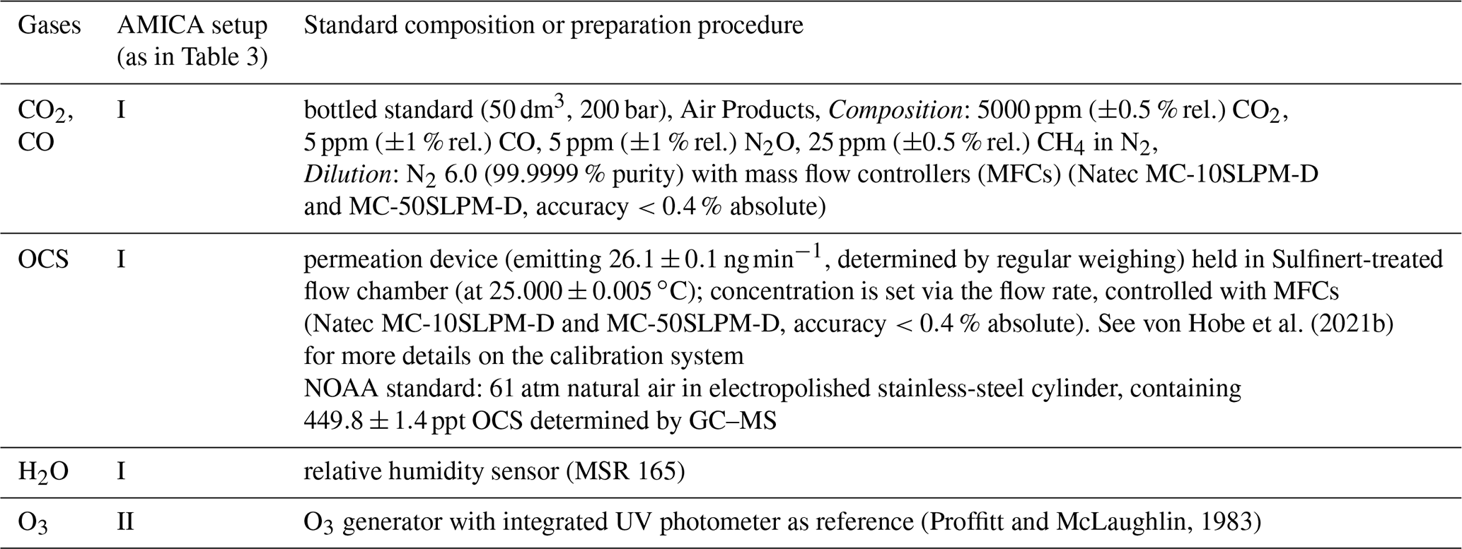
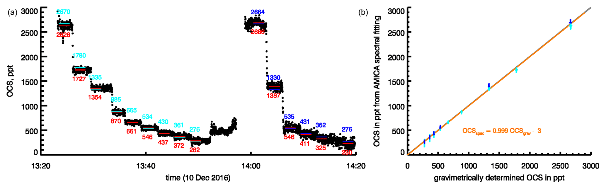
Figure 7 Laboratory calibration for AMICA OCS. (a) OCS mixing ratios fitted to AMICA spectra in black, with red bars and numbers indicating averages for each mixing ratio level. Mixing ratios of the standards are also shown as bars and numbers for a series at P_cav=46 hPa (light blue) and one at P_cav=18 hPa (dark blue). (b) Fitted AMICA OCS against the gravimetric standards with the same blue colours indicating P_cav of each measurement. Error bars in x direction represent the uncertainty of the gravimetric standards (propagated from uncertainties in permeation rate and flow rates); error bars in y direction represent the statistic measurement uncertainty determined at each mixing ratio. The 1:1 line is shown in grey, and a linear fit to all data (independent of P_cav) is shown in orange.

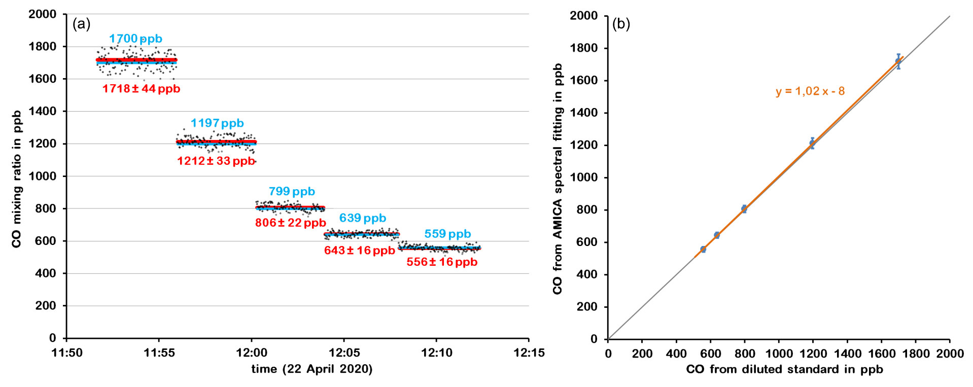
Figure 8 Panel (a) shows the CO mixing ratios fitted to AMICA spectra (black: individual data points; red: averaged with standard deviations) and the known mixing ratios in the standards (light blue) against time of the experiment. Panel (b) shows AMICA CO vs. standard CO and a linear fit of these data.

Results of laboratory calibrations against a series of known standards (a compilation of standards and standard preparation procedures used in this work is given in Table 5) are shown in Fig. 7 for OCS and in Fig. 8 for CO. For both gases, excellent agreement with the standards is achieved just using the HITRAN parameters for the Voigt fit; i.e. no calibration factors are used in the derivation of their mixing ratios from the spectra (cf. Sect. 3.2). Taking into account uncertainties in the measurement of cavity pressure and temperature, the known trace gas standards used and the spectral analysis procedure, accuracies better than 5 % are estimated for both OCS and CO. Due to uncertainties in the prepared standards at low CO mixing ratios (caused by both a large dilution ratio and the possible presence of residual CO of unknown concentration in the clean dilution gas), accuracy is estimated to be only better than 15 % at CO mixing ratios below 60 ppb. Figure 7 also shows good agreement between measured and standard OCS concentrations during calibrations carried out at reduced pressure, simulating the high-altitude range during the M55 Geophysica campaigns, suggesting that low cavity pressure does not cause systematic errors. It must be noted, however, that at such low pressures, precision significantly deteriorates (cf. Sect. 2.3) and low stratospheric OCS and CO mixing ratios cannot be detected anymore.

For CO₂, spectral fits in either intensity or absorption space using only HITRAN parameters fail to arrive at the mixing ratios of the standards used or those expected in atmospheric measurements. This is at least partly caused by the issue with the strong CO₂ absorption affecting the absorption path length, but we also note that, unlike the HITRAN parameters used for OCS and CO, the parameters for the CO₂ line used are not based on experimental data but on theoretical calculations and are therefore associated with higher uncertainties. As a result, an additional calibration factor, determined from calibrations against known standards, needs to be introduced when deriving CO₂ mixing ratios from spectral fits. As a result of the spectral fitting issues and the additional uncertainty of the calibration factor, the error margins of the AMICA CO₂ data are currently of the order of a few parts per million (ppm), much larger than those of other CO₂ instruments used during the field campaigns. Therefore, AMICA CO₂ measurements up to this point are not used for scientific purposes and are not part of any data files released for the campaigns. We plan to verify and/or adjust the HITRAN parameters for the CO₂ line at 2050.60 cm⁻¹ in a future laboratory experiment with low CO₂ concentrations that do not reduce the effective path length at different pressures and temperatures, and we will then use them in the full fitting algorithm described by Sayres et al. (2009), where the effect on path length is mathematically represented.

Precision is shown for OCS, CO and CO₂ in the form of Allen deviation plots determined from measuring one standard over a longer period (Fig. 9). For all three gases, precision can be improved at the cost of time resolution by averaging up to 1 or 2 min where the curves reach more or less pronounced minima. Because of the short time periods of 5 and 45 min used in these experiments, long-term precision caused by instrumental drifts over longer time periods cannot be ruled out, and the observed behaviour at averaging times longer than about 200 s appears to point into that direction, although it is not conclusive. A measurement of the same standard with the current AMICA configuration over a period of several hours will be carried out in future to further investigate the susceptibility towards long-term drifts. We also expect to achieve a further lowering of the σ curves in the future by further reducing electrical noise. For the OCS and CO observations made so far, respective precision estimates of 30 ppt and 3 ppb are made based on the higher 2 s value from the two experiments shown in Fig. 9. For CO₂, both curves exceed 1 ppm for all averaging times, which is another reason (besides the issues described above) for currently not releasing AMICA CO₂ data for scientific use.

Figure 9 Allen deviation plots for OCS, CO and CO₂ based on measurement of the same standard by AMICA over an extended period of time (45 min with 1 s time resolution in the laboratory test in December 2016, blue line, and 5 min with 2 s time resolution inside HALO at the start of the SouthTRAC campaign).

In the current setup, H₂O can only be detected at mixing ratios above 100 ppm. Comparison of mixing ratios derived from spectral fits based on HITRAN parameters with a relative humidity sensor (MSR 165) placed near the AMICA inlet showed agreement better than 4 % under different conditions (4000–30 000 ppm H₂O).

Because OCS is one of the main scientific interests of our research group, the 2050–2051 cm⁻¹ setup is typically used in AMICA in the cavity 1 position.

4.2 O₃ and NH₃ at 1033–1034 cm⁻¹

A quantum cascade laser (QCL, Hamamatsu), operated at 29.6 ^∘C and ramped over the current range 775–925 mA, emits light over the wavenumber range of 1033.21–1034.36 cm⁻¹. In this spectral window, absorption lines exist for O₃ (major absorption lines at 1033.24, 1033.35, 1033.68, 1033.86 and 1033.93 cm⁻¹) and NH₃ (major absorption lines at 1033.32 and 1034.01 cm⁻¹). A spectrum measured by this channel during the 2019 SouthTRAC deployment (Sect. 5.3) is shown in Fig. 10 together with a spectral fit in absorption space that uses HITRAN line parameters. The spectral fit does not closely reproduce the observed spectrum. First, significant absorption up to 0.01 between peaks points to either a bias in the used baseline or trace gas absorption by lines or bands that are not included in the HITRAN database. Second, the observed O₃ absorption peaks are broader than the fitted peaks. Possible explanations include inaccurate HITRAN parameters for the O₃ lines or cavity response broadening. Both baseline offset and the broader peaks will be further investigated in future laboratory experiments.

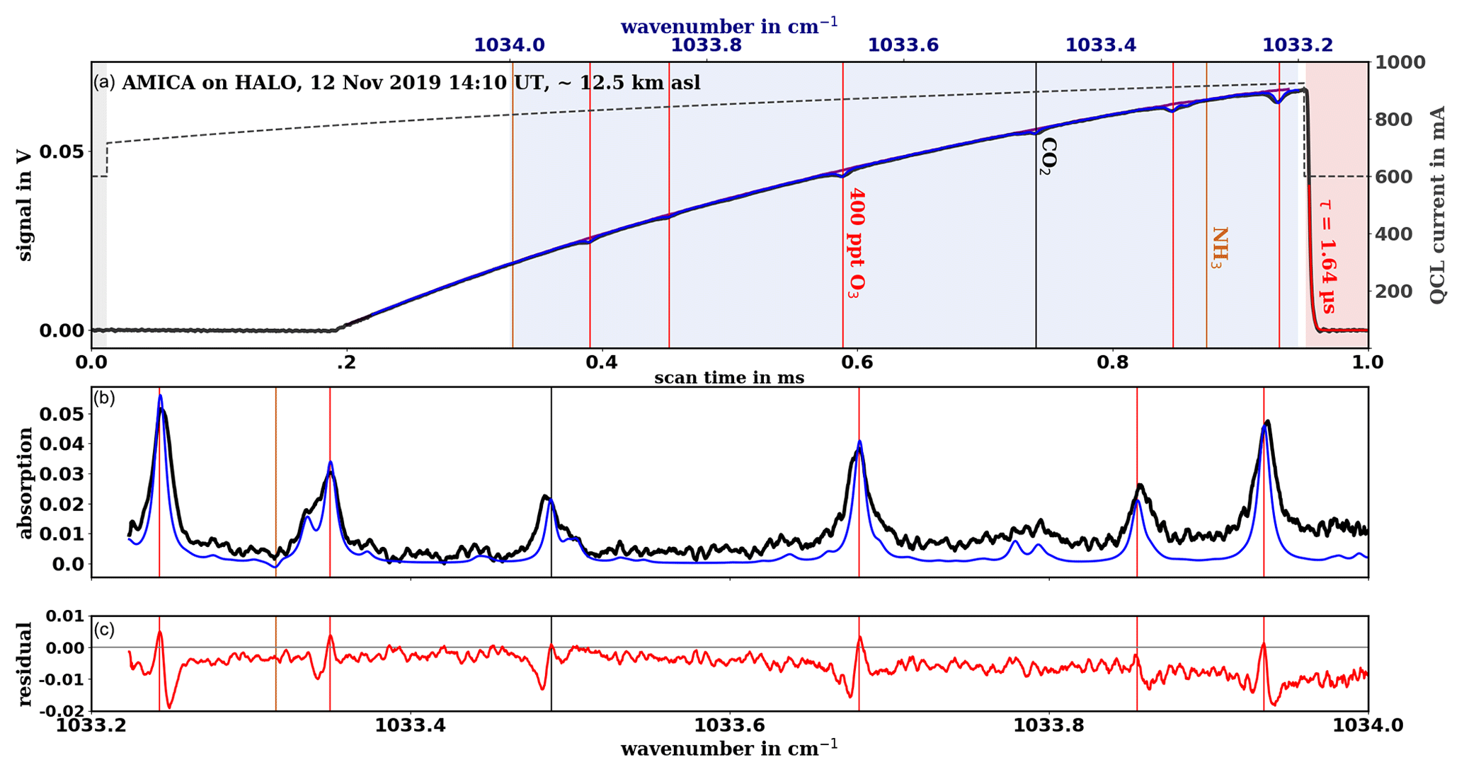
Figure 10 (a) QCL current (dashed line, right axis; the 775–925 mA ramp is slightly curved to arrive at the linear wavenumber scale indicated on the top x axis) and detector voltage signal past the preamplifier (solid black line, left axis; ramps averaged over 30 s) for AMICA cavity 2 in the 1034 cm⁻¹ setup. Three periods are marked by the coloured areas – (i) grey: only detector dark signal (with zero offset) is observed; (ii) blue: period used for spectral analysis; (iii) red: period after the QCL stops emitting, when the signal decays exponentially due to ring down of the light in the cavity. A ring-down fit is shown by the red line. For the spectral fitting region, a measured baseline spectrum with no absorbers present (purple) and a fitted spectrum (blue) are also shown. (b) Measured and fitted spectra from (a) shown in absorption space. (c) Difference between the fit and the measured spectrum (fitted–measured). Panels (b, c) only show data for the region that is actually fitted, i.e. the blue shaded region in (a). Absorption line positions coloured according to different gases are indicated in all panels by vertical lines for better comparison.

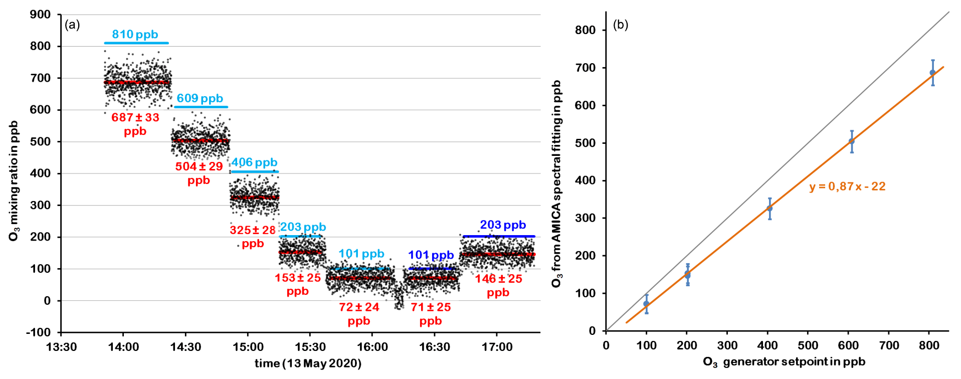
Figure 11 Panel (a) shows the O₃ mixing ratios fitted to AMICA spectra (black: individual data points; red: averaged with standard deviations) and the known mixing ratios in the standards (light/dark blue: with/without stainless-steel tube in transfer line; see text for details) against time of the experiment. Panel (b) shows AMICA O₃ vs. standard O₃ and a linear fit of these data.

A first set of laboratory tests to compare AMICA O₃ to known concentrations was carried out with an O₃ generator that accurately measures O₃ concentrations with an internal UV absorption spectrometer (Proffitt and McLaughlin, 1983). As shown in Fig. 11, AMICA underestimates O₃ mixing ratios. The reason for this underestimation is not yet fully understood. Obviously, the abovementioned issues with the spectral fitting of the O₃ spectrum affect the accuracy of the measurements, but Fig. 10 does not necessarily suggest an underestimation of the observed spectrum by the fit. A reason related to sampling rather than spectroscopy could be loss of O₃ inside the transfer line or the AMICA instrument, but we deem it unlikely for this to be the only reason. Inside AMICA, all surfaces are either Sulfinert^® or Teflon except for small stainless-steel parts inside the valves, and removal of a metal connector from the transfer line had no significant effect. We also note that for any particular mixing ratio, the AMICA response remains reasonably constant, and there we observed no significant difference going from low to high concentrations and vice versa. Sampling-related effects on the O₃ measurement will be further investigated in future experiments at different flow rates (this needs to be realized using an external pump and flow control). Another spectroscopic reason causing the bias could be inaccuracies in the wavenumber scale for this channel, which is locked to a significantly less prominent absorption feature than the CO₂ peak in the 2050–2051 cm⁻¹ channel.

In relative terms, the underestimation decreases with increasing mixing ratios, ranging from about 30 % at 100 ppb to 15 % at 800 ppb, but the response is linear overall, with a negative intercept of about 22 ppb (Fig. 11). Further tests and calibrations to better understand the reasons for the underestimation and to see if the response function is constant over longer periods of time and can thus be used as a correction function are planned. Based on the measurements shown in Fig. 11, the 0.5 Hz precision for O₃ is currently in the range of 20 to 40 ppb.

Significant absorption at the NH₃ line positions has not been detected during the SouthTRAC flights. Tests with a laboratory standard to investigate the sensitivity of this measurement are planned. Ultimately, it should be possible to measure NH₃ with similar sensitivity as described by Leen et al. (2013).

4.3 N₂O, HCN and C₂H₂ at 3331–3332 cm⁻¹

An interband cascade laser (ICL, Nanoplus), operated at 16.5 ^∘C and ramped over the current range 50.0–67.5 mA, emits light over the wavenumber range of 3330.6–3332.2 cm⁻¹. In this spectral window, N₂O (major absorption line at 3331.65 cm⁻¹), HCN (major absorption line at 3331.58 cm⁻¹) and C₂H₂ (major absorption line at 3331.33 cm⁻¹) can be measured.

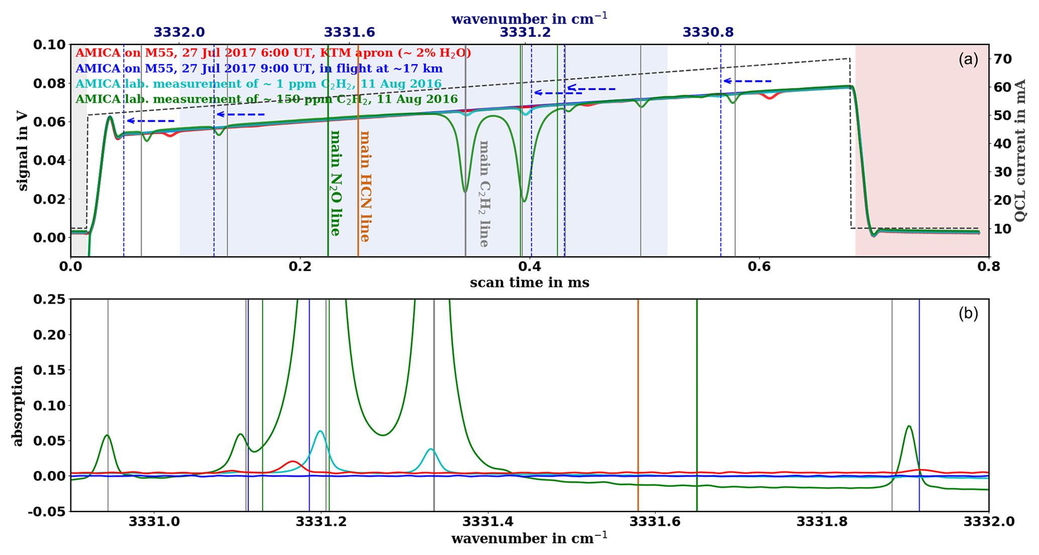
Figure 12 (a) QCL current (dashed line, right axis) and detector voltage signal past the preamplifier (left axis; ramps averaged over 300 s) for AMICA cavity 2 in the 3331 cm⁻¹ setup for a laboratory experiment sampling C₂H₂ from a bottle and a flight from Kathmandu (see legend for colours). The wavelength scale shown on the top axis was fitted to the laboratory data. The wavelength scale during the flights was shifted so that the observed H₂O peaks are relatively displaced (indicated by the dashed blue arrows). Three periods are marked by the coloured areas – (i) grey: only detector dark signal (with zero offset) is observed; (ii) blue: period for which absorption spectrum in the lower panel is shown; (iii) red: period after QCL stops emitting, when the signal decays exponentially due to ring down of the light in the cavity (the ring down was to fast to do a reasonable fit). (b) Measured spectra from (a) shown in absorption space (with the wavelength scale corrected). Absorption line positions coloured according to different gases are indicated in both panels by vertical lines for better comparison.

Figure 12 shows spectra recorded with this channel for diluted C₂H₂ from a gas bottle and on the ground and in-flight during the 2017 deployment from Kathmandu (Sect. 5.2). The pattern of the C₂H₂ peaks in the spectra from the gas bottle and of the H₂O peaks in the spectra taken at ground level in Kathmandu show that the OA-ICOS measurement in the desired wavelength region was successfully implemented. However, the decay of light intensity at the end of the ramp was too fast to obtain a useful ring-down fit. Based on the absorption obtained for the C₂H₂ mixing ratios used, mirror reflectivity is estimated to be only ∼0.995, corresponding to an effective path length of about 100 m. This is not sufficient to measure N₂O, HCN and C₂H₂ absorption at atmospheric concentrations, which is confirmed by the absence of absorption features in the spectra recorded at high altitude during the 2017 deployment in Nepal (Sect. 5.2). A mirror reflectivity of at least 0.9995 and probably a higher output ICL are needed to implement such atmospheric measurements, and we hope to test this with AMICA in the near future.

5 In-flight performance

To date, AMICA has been operated in the field during three aircraft campaigns. Between them, the instrument has undergone major technical modifications to continuously improve in-flight performance. Because a full description of each individual setup with referencing of all individual components would render this paper extremely lengthy, the technical description in Sects. 2 and 3 is limited to the current optimized version. To convey a broad sense for the “learning curve” during this instrument development phase and as a reference for scientists working with the AMICA campaign data (most of which is or will be freely accessible) or with published scientific results (e.g. von Hobe et al., 2021a), reference to setups or used parts different from the description in Sects. 2 and 3 will be given for each campaign.

5.1 M55 Geophysica, Kalamata, 2016

The very first aircraft deployment of AMICA took place in Kalamata, Greece, with three flights in late August or early September 2016. A major aspect of this campaign, which was part of the European StratoClim project (Stroh et al., 2021), was to test several new or modified instruments in the M55 Geophysica payload.

At the time, two separate PC/104 stacks were used, one for each of the two ICOS systems. Acquisition and A/D conversion of the voltage signals from C9a/b was handled by a board inside each PC/104 stack, and averaging was done by the software running on the PC. The data acquisition boards were also used to generate voltage ramps that were passed on to the laser controllers used at the time (RedWave Labs) for current modulation. Temperature regulation of lasers, laser mounts and detectors was done by separate TEC controllers (Wavelength Electronics).

AMICA operated and produced useable data during each flight, but the data quality – precision in particular – was significantly reduced compared to the current instrument (i.e. as described in Sects. 2 and 3), mainly for two reasons:

• i.

  Cavity pressure fell below the set point of controller C3b (42.5 hPa during this campaign) at an altitude around 14 km and was significantly lower than shown in Fig. 4 for any given ambient pressure. This was largely caused by the flow resistance of two particle filters (Swagelok F series), which was remedied by replacing the filters by high-flow versions (Swagelok FW series) before the third flight, in which cavity pressure regulation worked nominally up to about 16.5 km altitude. Above this altitude, the pressure drop between measured ambient and cavity pressure was still significantly larger than in the laboratory experiment (described in Sect. 2.4 and shown in Fig. 4). The likely reason for this is a significantly negative pressure coefficient at the dome on top of the M55 Geophysica aircraft during flight leading to an effective surface pressure at the inlet position up to 30 hPa below static pressure. This is supported by the observations of similarly lower than expected pressures in another instrument connected to an inlet directly adjacent to the AMICA inlet and by a significant variability of the pressures in both instruments with the aircraft's angle of attack that is known to affect pressure coefficients at the aircraft surface from fluid dynamics considerations. As stated in Sect. 2.3, lower cavity pressure reduces the trace gas absorption signals and therefore instrument precision.

• ii.

  The second precision limiting factor is noise. The sophisticated clean power and grounding concept described in Sect. 2.5 had not been fully implemented in 2016, and ground loops as well as devices with a variable power draw (e.g. valves, fans, TEC controllers) connected to the same DC source induced noise at the data acquisition card in the two PC/104 stacks used at the time.

Another critical issue during this campaign was a tendency for overheating of the powerbox during the instrument warm-up phase on the apron prior to take-off. When AMICA was turned on, temperature at the three VIPAC converters (V1–V3) and near the centre of the powerbox rose above 80 ^∘C within minutes. The values could be monitored in real time via Wi-Fi connection, and it was decided to manually turn AMICA off to prevent damage. AMICA was turned back on only just before take-off so that the ICOS enclosure temperature and consequently the spectral signal only fully stabilized well into the flight. During flight, the air stream around the instrument proved sufficient to prevent powerbox overheating. Post-campaign tests revealed the major part of the heat load inside the powerbox to come from 2×60 W heat dissipation by two boards controlling the TEC assemblies regulating enclosure temperature. The problem of overheating on the apron was remedied by the selection of different TEC controller boards (D7a/b in Table 2) with a maximum heat dissipation of ∼10 W at maximum load each.

5.2 M55 Geophysica, Kathmandu, 2017

A second deployment on the M55 Geophysica was also part of the StratoClim project and is described by Stroh et al. (2020). Eight research flights took place from Kathmandu, Nepal, between 27 July and 10 August 2017 to analyse the chemical composition as well as transport and mixing processes within the Asian summer monsoon (ASM) anticyclone. AMICA data for all flights are available (see “Data availability” section below) and a scientific analysis of vertical transport within the ASM anticyclone that uses AMICA CO data has recently been published (von Hobe et al., 2021a).

Some of the issues described in Sect. 5.1 were still not fully resolved. While the use of the high-flow filters resulted in the nominal characteristics of the flow system described in Sect. 2.4 with pressure drops as shown in Fig. 4, the reduced effective pressure at the inlet on the aircraft surface was unavoidable. This means that instrument precision worsens with absorption signals as pressure drops above 16.5 km flight altitude. This is particularly relevant for the measurement of OCS that absorbs only weakly at atmospheric concentrations. Electrical noise was reduced compared to the 2016 campaign by rewiring a few particularly critical components (in terms of power draw variability, e.g. valves), but the comprehensive power and grounding concept described in Sect. 2.5 was only implemented after this campaign. Another issue encountered during the Kathmandu deployment was related to laser temperature control, which at the time was done by different controllers that received their set point from the PC via an analogue 0–10 V signal. Both fluctuations and drifts were encountered that affected the position of the spectral window and introduced additional uncertainties in the assignment of the wavenumber scale to each measured spectrum, making the spectral analysis difficult.

5.3 HALO, SouthTRAC, 2019

The first AMICA deployment on the German HALO took place during the SouthTRAC mission in 2019 (Rapp et al., 2020; also see https://www.pa.op.dlr.de/southtrac/, last access: 22 July 2021). The payload was integrated in Oberpfaffenhofen, Germany, in July and August. The main campaign base was in Rio Grande, Argentina, where local science flights were carried out in two phases in September and November. Transfer flights with stops in Sal on the Cabo Verde islands and Buenos Aires, Argentina, were carried out in early September, early October and early November.

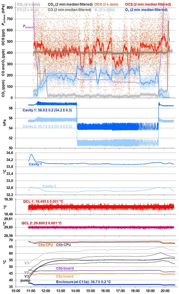
Figure 13 From top to bottom: AMICA trace gas observations, cavity pressures and temperatures, QCL temperatures, and other selected temperatures in the enclosure and powerbox recorded during the SouthTRAC flight on 12 November 2019 from Rio Grande, Argentina.

AMICA was situated in a rack near the front of the aircraft cabin. For SouthTRAC, it was flown with the fully implemented power and grounding concept and a revised design of the ICOS control and data acquisition as described in Sects. 2 and 3. Cavity pressure regulation worked nominally up to the HALO ceiling altitude of about 15 km. Except for two short test flights in Oberpfaffenhofen in August, where the recorded spectra were not correctly stored to disk due to a software problem, AMICA operated and recorded data during all flights. Towards the end of the long transfer flights at the beginning of the campaign, some data gaps are present that were caused by incidental shut offs of the LTC-1141 boards C6a and C6b to prevent overheating. A close examination of this issue at the campaign base in Rio Grande revealed that the NTC sensors of the two large TEC boards (Fig. 2) were incorrectly connected, causing them to work against each other and not sufficiently cool the ICOS enclosure. By swapping the NTCs into their correct positions (as shown in Fig. 2), the problem was solved. Figure 13 shows observed trace gas mixing ratios and selected housekeeping data for the SouthTRAC flight on 12 November 2019 when AMICA operated nominally over the entire flight. The figure nicely illustrates the excellent stability of cavity pressures (middle panel) and enclosure as well as QCL temperatures (bottom panel). Kloss et al. (2021) have used CO observations from this flight to identify a plume originating from bush fires in Australia.

6 Conclusions

With AMICA, an automated airborne OA-ICOS analyser has been developed that fully complies with all mechanical and electronic airworthiness requirements and that has successfully been deployed in three measurement campaigns on two very different aircraft. A number of distinct or even unique design features are particularly innovative:

• A single instrument housing contains two discrete OA-ICOS cavities, allowing for the simultaneous measurement of a wider range of different species in two different wavenumber regions. The two ICOS systems share a common power supply system and control PC.

• By exchanging only cavity mirrors, laser source and detector, the target wavenumber region of each OA-ICOS setup can be switched, and the suite of species measured by AMICA can to some extent be tailored to the scientific questions of a particular campaign. When a particular campaign or aircraft protocol provides for temporary dismounting and modifications of instruments, the exchange of an OA-ICOS cavity in AMICA can even be carried out during a campaign within approximately 1 working day.

• The flow system with two parallel valves with different orifices provides precise regulation of cavity pressures over the wide range of ambient pressure encountered between ground and maximum flight altitude.

• The containment of the sensitive OA-ICOS hardware in a pressure-sealed and thermally controlled enclosure allows for deployment outside the aircraft cabin, i.e. in instrument bays exposed to the low pressure and low temperature conditions at flight altitudes up to at least 20 km. To seal the large rectangular enclosure, an adhesive was applied to the surfaces where individual plates were bolted together.

Further deployments of AMICA in future airborne campaigns are planned. Currently, work is being done to further improve the signal-to-noise ratio, e.g. by filtering the zero offset signal from the PC to the preamplifier. It is also planned to install mirrors with higher reflectivity and possibly an ICL with higher power output for the 3331 cm⁻¹ channel to render it suitable for measuring N₂O, HCN and C₂H₂ at atmospheric concentrations. It is also envisaged to eventually add further channels at different wavenumber regions to AMICA in order to target additional trace gases, depending on the science questions of future missions.