the Creative Commons Attribution 4.0 License.
the Creative Commons Attribution 4.0 License.
 | 27 Jan 2021
Empirically derived parameterizations of the direct aerosol radiative effect based on ORACLES aircraft observations
Sabrina P. Cochrane
K. Sebastian Schmidt
Hong Chen
Peter Pilewskie
Scott Kittelman
Jens Redemann
Samuel LeBlanc
Kristina Pistone
Meloë Kacenelenbogen
Michal Segal Rozenhaimer
Yohei Shinozuka
Connor Flynn
Amie Dobracki
Paquita Zuidema
Steven Howell
Steffen Freitag
Sarah Doherty
In this paper, we use observations from the NASA ORACLES (ObseRvations of CLouds above Aerosols and their intEractionS) aircraft campaign to develop a framework by way of two parameterizations that establishes regionally representative relationships between aerosol-cloud properties and their radiative effects. These relationships rely on new spectral aerosol property retrievals of the single scattering albedo (SSA) and asymmetry parameter (ASY). The retrievals capture the natural variability of the study region as sampled, and both were found to be fairly narrowly constrained (SSA: 0.83 ± 0.03 in the mid-visible, 532 nm; ASY: 0.54 ± 0.06 at 532 nm). The spectral retrievals are well suited for calculating the direct aerosol radiative effect (DARE) since SSA and ASY are tied directly to the irradiance measured in the presence of aerosols – one of the inputs to the spectral DARE.
The framework allows for entire campaigns to be generalized into a set of parameterizations. For a range of solar zenith angles, it links the broadband DARE to the mid-visible aerosol optical depth (AOD) and the albedo (α) of the underlying scene (either clouds or clear sky) by way of the first parameterization: P(AOD, α). For ORACLES, the majority of the case-to-case variability of the broadband DARE is attributable to the dependence on the two driving parameters of P(AOD, α). A second, extended, parameterization PX(AOD, α, SSA) explains even more of the case-to-case variability by introducing the mid-visible SSA as a third parameter. These parameterizations establish a direct link from two or three mid-visible (narrowband) parameters to the broadband DARE, implicitly accounting for the underlying spectral dependencies of its drivers. They circumvent some of the assumptions when calculating DARE from satellite products or in a modeling context. For example, the DARE dependence on aerosol microphysical properties is not explicit in P or PX because the asymmetry parameter varies too little from case to case to translate into appreciable DARE variability. While these particular DARE parameterizations only represent the ORACLES data, they raise the prospect of generalizing the framework to other regions.
- Article
(5448 KB) - Full-text XML
- Companion paper
- BibTeX
- EndNote


During the African burning season of August–October, a semi-permanent stratocumulus cloud deck off the southern African western coast is overlaid by a thick layer of biomass burning aerosols. These aerosols are advected over the southeast Atlantic Ocean from the interior of the African continent and account for nearly one-third of the total global biomass burning aerosol (van der Werf et al., 2010). The seasonal environment of high biomass aerosol loading above clouds has large, variable radiative impacts that have yet to be fully characterized.
In addition to many other science objectives, the NASA ORACLES aircraft campaign aimed to obtain the direct aerosol radiative effect (DARE) in both cloudy and clear skies for this region (Zuidema et al., 2016; Redemann et al., 2020). The distinction between DARE in cloudy vs. clear skies is crucial since the albedo below an aerosol layer strongly influences the sign and magnitude of DARE. The albedo from below an aerosol layer can determine the sign of the top of the atmosphere (TOA) DARE independently of the aerosol itself (Twomey, 1977; Hansen et al., 1997; Russell et al., 2002; Keil and Haywood, 2003; Yu et al., 2006; Chand et al., 2009; Zhang et al., 2016; Meyer et al., 2013, 2015). In a region like the southeast Atlantic, this makes determining DARE challenging since the cloud fields change rapidly according to the flow of the marine boundary layer. Depending on the cloud albedo, the aerosol could be warming (positive DARE) or cooling (negative DARE) at the TOA (Yu et al., 2006; Russell et al., 2002; Twomey, 1977). The albedo value where DARE transitions from positive to negative, or warming to cooling, is known as the critical albedo (Haywood and Shine, 1995; Russell et al., 2002; Chand et al., 2009).
The spectral DARE in W m−2 nm−1 is determined from the difference between the net irradiance () with and without the aerosol layer:
Aircraft measurements, such as those collected during ORACLES, provide direct observations of the components necessary to calculate DARE. However, measurements are only taken for a sub-sample in time and space and may not be representative of the region as a whole. DARE calculated from aircraft observations alone would therefore leave the larger question of whether the aerosols warm or cool the southeast Atlantic unanswered.
In the case of DARE, the translation from individual observations into a common framework was first introduced by Meywerk and Ramanathan (1999). The radiative forcing efficiency (RFE) empirically relates DARE to the aerosol optical depth (AOD):
The RFE is defined as the (usually broadband) DARE normalized by the (usually mid-visible) AOD or sometimes as the derivative of DARE with respect to the AOD. It can be regarded as an intensive property of an air-mass that allows the direct conversion from AOD to DARE, complementing calculations based on aerosol microphysical and optical properties. When the RFE is aggregated for an entire field mission, it can provide a representative air-mass characteristic that lends aircraft observations a broader scientific impact than the contributing individual measurements. If aerosol microphysical and optical properties are insufficiently known in a region of interest, this mission-aggregated RFE constitutes a DARE parameterization that solely requires AOD (Eq. 2). If the RFE varies little in a region and season of interest, it can be used to derive regional DARE estimates via AOD statistics from satellites – at least in principle. More fundamentally, observations of the dependence of flux changes on AOD help to develop confidence in radiative forcing calculations based on measured aerosol properties (Russell et al., 1999; Redemann et al., 2006). In this sense, the RFE in conjunction with Eq. (2) provides closure to those calculations and thus constrains them from the radiative flux and DARE perspective.
In this paper, we generalize the concept of RFE by explicitly taking into account the dependencies of DARE not only on AOD as expressed in Eq. (2), but also on both the aerosol and cloud properties. ORACLES measurements are used collectively to develop two parameterizations of instantaneous DARE in the form of
and
where AOD, α, and SSA are the aerosol optical depth, albedo, and single scattering albedo at 550 nm. The 550 nm albedo is the albedo of the scene below the aerosol layer (open ocean and/or cloudy scene), and the SSA is a measure of aerosol absorption. P stands for the two-parameter representation of DARE and PX stands for an extended version with three parameters. Both parameterizations provide instantaneous broadband DARE that is based upon spectral aerosol and cloud properties. The right-hand sides of Eqs. (3) and (4) are mid-visible quantities, while the left-hand sides are broadband results. The parameterizations have the advantage of implicitly accounting for the spectral dependencies of the aerosol and cloud properties (e.g., aerosol scattering phase function, aerosol vertical distribution, spectral dependence of aerosol absorption, cloud optical depth, cloud effective radius, cloud top and base height), whereas the dependence on mid-visible AOD, SSA, scene albedo, and solar zenith angles is explicit. They are not meant to replace detailed or approximated radiative transfer calculations (e.g., Coakley and Chylek, 1975), which would require all of these inputs, but rather to arrive at a broadband DARE with a minimum set of input parameters that drive its regional variability.
From the user standpoint, applying the parameterizations is straightforward because broadband DARE can be estimated with minimal information on the cloud and aerosol properties. The parameterization coefficients encompass the many complexities of transitioning from narrowband to broadband, such that the spectral dependencies of the cloud and aerosol properties are not necessary. Of course, the parameterization only represents the “mean” conditions encountered in the ORACLES region and sampling time, and it becomes invalid outside of this mission envelope. Equation (3) only requires AOD and scene albedo at mid-visible 550 nm, which can be readily obtained from satellite observations. If mid-visible SSA is also known (from satellite or aircraft retrievals, from in situ observations, or from a climatology), the second parameterization (Eq. 4) can be used, which decreases the uncertainty of DARE, as we will discuss below.
To arrive at the final parameterizations, we first build upon the method presented in Cochrane et al. (2019, further denoted as C19) and determine the aerosol intensive properties of SSA and asymmetry parameter (g) that best represent the ORACLES region during August and September of 2016 and 2017. We evaluate the radiative effects of those aerosols where the relationships found between DARE, AOD, and albedo form the foundation of the parameterizations that capture the collective variability sampled from the viable cases from ORACLES 2016 and 2017.
The paper has two parts, which can be read independently depending on the reader's main interest. In the first part (Sect. 2), we describe the data and the methods used to determine spectrally resolved SSA and g. We generalize earlier work (C19) by adding a methodology for a uniform processing of multiple cases. The second part (Sect. 3) translates AOD, albedo, and SSA into DARE, and the P and PX parameterizations are constructed by progressively capturing more of the case-to-case DARE variability. In Sect. 5, we provide a quick summary and interpretation of both parts of the paper.
2.1 Data
The ORACLES project conducted research flights in the southeast Atlantic for three 1-month periods over 3 consecutive years (2016–2018) during the burning season to study the biomass burning aerosols and stratocumulus cloud deck. To achieve the defined science objectives, the ORACLES project made use of the NASA P-3 aircraft for the duration of the experiment and the NASA ER-2 aircraft in 2016 only. Between the 2016 and 2017 deployments, the P-3 completed 26 science flights, 5 of which were collocated with the ER-2. All data can be found on the NASA ESPO archive website (ORACLES Science Team, 2017, 2019).
We focus on utilizing measurements taken from the P-3, primarily the irradiance measurements taken by the Solar Spectral Flux Radiometer (SSFR, Pilewskie et al., 2003; Schmidt and Pilewskie, 2012) in conjunction with AOD and retrievals of column gas properties from the Spectrometer for Sky-Scanning Sun-tracking Atmospheric Research (4STAR, Dunagan et al., 2013; Shinozuka et al., 2013; LeBlanc et al., 2020) to achieve the specific goals of this paper. SSFR consists of two pairs of spectrometers. Each pair (one zenith viewing and one nadir viewing) covers a wavelength range of 350–2100 nm. SSFR is radiometrically and angularly calibrated pre- and post-mission. Its zenith light collector is equipped with an active leveling platform (ALP), which keeps it horizontally aligned by counteracting the variable aircraft attitude. This allows the collection of irradiance data as long as pitch and roll stay within the ALP operating range of 6∘. This ensures that radiation from the lower hemisphere does not contaminate the zenith irradiance measurements, which was especially important for the bright clouds encountered during ORACLES. 4STAR provides spectral retrievals of AOD from the solar direct beam irradiance above the aircraft and is calibrated through the Langley extrapolation technique before and after deployment at Mauna Loa Observatory along with in-flight high-altitude measurements (see LeBlanc et al., 2020, for details on 4STAR calibration). 4STAR also provides aerosol intensive properties (e.g., SSA described in Pistone et al., 2019) and column water vapor and trace gas retrievals, such as ozone (e.g., Segal-Rosenheimer et al., 2014). Further details on SSFR, ALP, and 4STAR instrumentations and calibrations can be found in C19.
2.2 Methods
To construct our DARE parameterizations, aerosol intensive optical properties such as SSA and g must be determined for as many cases as possible. Retrieving these properties from aircraft irradiance measurements is inherently challenging because the aerosol radiative effects can be relatively small compared to the horizontal variability of cloud albedo.
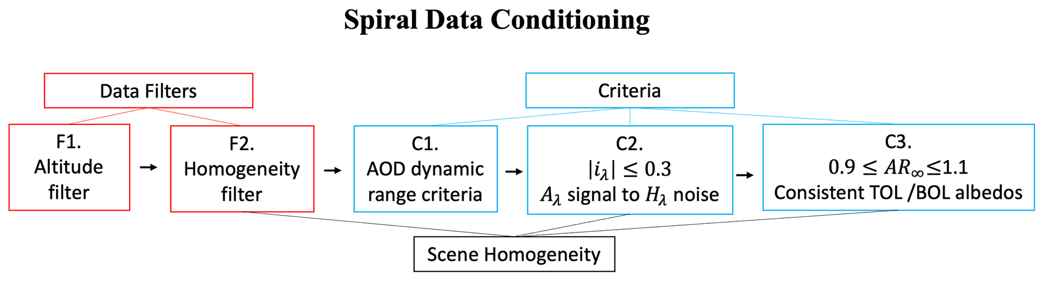
Figure 1Data conditioning flowchart. First, the data are filtered vertically (i.e., data are removed) to (F1) isolate the aerosol layer only and (F2) isolate either cloudy- or clear-sky data such that the profile represents a homogeneous sky type. Once filtered, the data must pass three distinct criteria to ensure that (C1) the full aerosol layer is captured, (C2) the effect of aerosol absorption on radiative fluxes is much greater than that due to horizontal variability present, and (C3) the top-of-layer (TOL) and bottom-of-layer (BOL) albedos are mutually consistent.
C19 showed for two cases that special spiral maneuvers (“square” spiral) are more successful than the heritage “stacked leg” approach because multiple measurements are taken throughout the vertical profile over a short time period (typically 20 min). This sampling strategy reduces the effects of cloud inhomogeneities and allows isolation of the aerosol signal, as long as specific quality criteria (detailed below) are met. These criteria, preceded by two filtering steps in which data points are removed, are described in the following section and follow the order presented in the flowchart of Fig. 1. The filters and criteria provide objective data conditioning prior to the subsequent aerosol retrieval and DARE parameterizations.
2.2.1 Data conditioning
Throughout the spiral, the zenith (downwelling) and nadir (upwelling) irradiance measurements are continuously affected by the aerosol layer. The aerosol-induced changes to the irradiance profiles allow us to extract information about the aerosol itself. As can be seen in Fig. 2a, both upwelling () and downwelling () irradiance profiles have an approximately linear relationship with AOD due to the absorption and scattering of the aerosol layer. Any deviation from the linear relationship is attributed to changes in the underlying cloud; these are filtered out to isolate the radiative effect of the aerosol. This linear assumption for the global downwelling is a simplification only for initial fitting for the subsequent filtering, and deviations from the linear relationship could be due to non-linearities as expected from Beer's law or vertical dependencies of aerosol parameters. However, we expect these to be negligible compared to changes in the underlying clouds and therefore use deviations from a linear profile to filter our data.
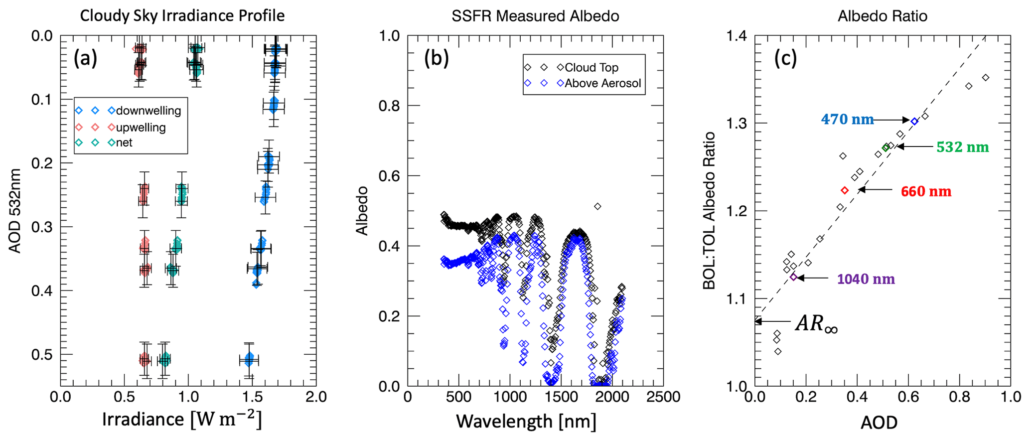
Figure 2(a) Above cloudy sky upwelling, downwelling, and net irradiance profiles shown vs. the 532 nm AOD measured by 4STAR with associated measurement error bars for one example case. The AOD refers to the air above the aircraft and generally decreases with increasing aircraft altitude, hence the inverted y axis. (b) SSFR-measured albedo spectrum at the bottom of the spiral (cloud top) and at the top of the spiral (above the aerosol layer). (c) The ratio between the BOL and TOL albedo spectra (taken from Fig. 2b) shown against the BOL AOD spectrum at the 4STAR wavelengths. The intercept of the fit line is criterion 3 (AR∞); if the intercept deviates largely from 1.0, the case cannot be used for an aerosol retrieval. Select wavelengths are labeled to highlight the spectral importance of this method.
Following the methods described in C19, two filters are applied to the data to ensure the isolation of aerosol effects. Prior to filtering, all data are corrected to the SZA at the midpoint of the spiral according to Eq. (3) in C19 to account for the minor change in solar position throughout the spiral. The first is an altitude filter (see F1 in Fig. 1), where the altitude range is limited to encompass only the vertical extent of the aerosol layer. The second is a homogeneity filter (see F2 in Fig. 1), which selects the dominant profile of measurements, whether that be cloudy or clear sky, and removes any outlying data. The filter begins with a linear fit of the irradiances with respect to the AOD for each wavelength:
where aλ and bλ (cλ and dλ) are the slope and intercept of the linear regression, for which the individual data points are weighted inversely by the irradiance uncertainties. In any particular spiral, the measurements could be taken from either predominantly cloudy or clear sky. The filter, which is applied to the upwelling profile, retains only those data within the 68 % confidence interval (1σ) of the linear fit line. This ensures that the retained data contain no outlying points and are all from one mode: clear sky or cloudy sky. This filtering step is slightly modified from the method presented in C19 in two ways: (1) the irradiances were previously fit against AOD at 532 nm only rather than AOD at the corresponding wavelength and (2) the range of retained data was previously based on the confidence interval of the overall mean irradiance value rather than the confidence interval of the linear fit throughout the profile. We have made these adjustments to better allow for linear variation with altitude while eliminating data that significantly deviate from the profile. There are three exception cases for which we maintain the original filtering from C19 using the confidence interval on the mean value. For these cases, the filtering modification overly eliminated data or retained excessive variability at small (large) AOD values (high altitude (low altitude)).
Following the filters, each case must pass criteria that ensure the changes in net irradiance with altitude are caused by the aerosol radiative effects and not variability in the underlying cloud field. First, irradiance measurements must be available throughout the spiral, spanning the full AOD dynamic range between the top and bottom of the layer (C1 in Fig. 1). The most common reason for cases to fail this criterion is that the AOD never reaches background stratospheric AOD levels (near zero; 0.02–0.04 in the mid-visible), indicating measurements were not taken fully above the aerosol layer. Since the retrieval relies on the change in irradiance with altitude, incomplete profiles do not provide a sufficient change required to capture the aerosol signal.
The second requirement (C2 in Fig. 1) is to ensure that the true aerosol absorption be larger than the 3-D cloud effect known as horizontal flux divergence (see Fig. 1 in C19). SSFR actually does not measure the absorption directly, but rather the decrease in the net flux from the top of the aerosol layer (TOL) to the bottom (BOL), or vertical flux divergence:
which we normalized by the incident irradiance. Vλ is only the vertical part of the total flux divergence. The other part is the horizontal flux divergence, Hλ, which is not measured by SSFR. The true absorption, Aλ, is obtained from the total flux divergence:
If the condition (see Sect. 3.1.2 in C19), then Aλ≈Vλ, and the vertical flux divergence measured by SSFR can be used in lieu of the true absorption. The first step to check that this requirement is met is to calculate Vλ from the linear fit in Eqs. (5) and (6):
where is the AOD at the bottom of the spiral (just above the cloud), and aλ and bλ are the slope and intercept of the linear fit lines. The second step is to estimate Hλ. Neglecting its weak wavelength dependence (Song et al., 2016), we instead use H∞, the value of Hλ at large wavelengths. As described in C19, H∞ can be determined using measurements of AODλ and Vλ: the AOD decreases with increasing wavelength, and therefore the true aerosol absorption decreases as well; as AODλ reaches zero, so does Aλ. When this happens, any non-zero measured value of Vλ must originate from Hλ because . Since this occurs at long wavelengths, the vertical flux divergence Vλ⟶∞ yields H∞. In practice, we obtain H∞ from the intercept of the regression between AODλ and Vλ.
To determine the relative amount of absorption to horizontal flux divergence, C19 developed a unitless metric (iλ) that determines whether the case is viable for an aerosol retrieval. iλ is defined as
If iλ>0.3, then the condition is not met, and the case is not considered viable for a subsequent retrieval.
The final criterion (C3 in Fig. 1), the measured albedo at the cloud top (bottom of layer – BOL) and above the aerosol layer (top of layer – TOL) shown in Fig. 3b, must be consistent in the limit of zero AOD. As the aerosol absorption decreases with increasing wavelength, the ratio between the measured albedo at the cloud top (BOL) and above the aerosol layer (TOL) must shift closer and closer to 1. Analogous to the determination of H∞ and illustrated in Fig. 2c, we determine AR∞ as the intercept between the TOL and BOL albedo ratio and the AOD.
In the limit of λ→∞,
AR∞ is our final criterion, and any deviation larger than 0.1 from 1.0 (i.e., the intercept must fall between 0.9 and 1.1) indicates that other factors affect the data besides the aerosol absorption. For example, a changing cloud field could change the albedo between the beginning and end of the spiral, and the aerosol retrieval might wrongly attribute this change to aerosol absorption.
To summarize, the criteria each case must pass are the following:
- C1.
There must be valid data from both SSFR and 4STAR throughout the entire aerosol profile. Cases cannot be used within the retrieval if there is a lack of data due to aircraft flight pattern, ALP malfunction, or AOD data flagged for bad quality.
- C2.
must be below 0.3 to ensure that the aerosol absorption is large enough compared to the horizontal flux divergence so that an aerosol retrieval is possible.
- C3.
AR∞ must fall between 0.9 and 1.1 to ensure that the spectral albedo is consistent both above and below the aerosol layer.
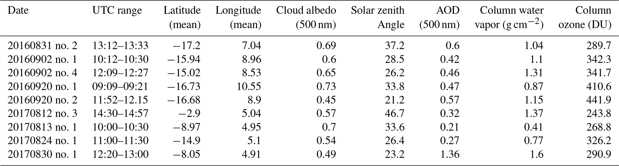
Both the filters and the criteria are designed to control for any rapidly changing, potentially inhomogeneous cloud field encountered during ORACLES. Table 1 presents the C2 and C3 criteria and retrieval status of SSAλ and gλ for spiral cases completed in 2016 and 2017 that passed C1. In 2016, 5 spiral profiles out of 18 met all criteria, while 4 out of 23 met the criteria in 2017. Table 2 provides the UTC, latitude, and longitude ranges for each successful spiral profile.
Table 1Retrieval quality metrics. Spirals are listed by date and the number in which they were performed on a particular flight. Spiral cases that did not have data spanning the entire aerosol layer are excluded from the chart (i.e., did not pass criterion no. 1). The second column lists the longest wavelength for which iλ remains below 0.3; the aerosol retrieval is only valid up to this wavelength. If iλ at all wavelengths is greater than 0.3, the case fails completely. The third column lists the AR∞ value. The intercept must fall between 0.9 and 1.1 to pass this metric. The right-most column provides the status for the retrieval of SSAλ and gλ. Cases that are analyzed using the mean fit rather than the updated linear fit (update 2 from C19) are indicated by *. Cases that pass a metric but have a bad spectral shape in the albedo ratio (indicating failure) are indicated by **.

Table 2Spiral case details for successful aerosol retrievals. The albedo, SZA, AOD, column water vapor, and column ozone are used within the radiative transfer model to retrieve aerosol properties and calculate DARE. The AOD, water vapor, and ozone are all reported above cloud.
2.2.2 Retrieval algorithm
If a spiral irradiance profile has passed every criteria metric, the aerosol property retrieval is run. The retrieval, described in detail in C19, is based on statistical probabilities between the calculated model irradiance profiles and the measured irradiance profiles. The retrieval process is similar to curve fitting, where we vary the parameters in question (i.e., SSA and g) until the radiative transfer model (RTM) calculations best fit the measured data.
The SSA and g retrieval is performed with the publicly available one-dimensional (1-D) RTM DISORT 2.0 (Stamnes et al., 2000) with SBDART for atmospheric molecular absorption (Ricchiazzi et al., 1998) within the libRadtran library (Emde et al., 2016; http://libradtran.org, last access: 21 January 2021). The RTM is run with six streams, assumes a Henyey–Greenstein phase function, and no delta-Eddington scaling is applied, all of which contribute to the inherent uncertainty within the RTM (Boucher et al., 1998). For each wavelength, we use the RTM to progress through pairs of SSA and g and calculate the upwelling, downwelling, and net irradiance profiles for each pair. For each {SSA, g} pair calculation, a probability is assigned to every SSFR data point in the profile according to the difference between the calculation and the measurement based on an assumed Gaussian distribution that represents the SSFR measurement uncertainty. The overall probability of a specific {SSA,g} pair given the SSFR irradiance measurements is the product of the individual probabilities for each data point; the {SSA,g} pair with the highest overall probability between all three profiles (upwelling, downwelling, net) is the retrieval result for that wavelength. The inclusion of the net profile is an expansion upon the method described in C19. The net irradiances provide a direct absorption constraint on the SSA retrieval, whereas the asymmetry parameter retrieval draws primarily upon the upwelling and downwelling fluxes.
In addition to the aerosol property pairs of {SSA,g}, the RTM ingests the spectral cloud top albedo from SSFR (set as the surface within the model at the measured altitude, around 2 km) and the aerosol extinction profile derived from the 4STAR AOD profile. The AOD profile has been conditioned such that the profile decreases monotonically to eliminate any unphysical extinction values (i.e., negative extinction). Any remaining AOD above the aerosol layer is allocated to a layer extending to an altitude of 15 000 m.
We modified the standard tropical atmosphere included in the libRadtran package (Andersen et al., 1986) to include the column water vapor measurements taken by the NASA P-3 hygrometer from the level of the cloud top to the maximum altitude of the spiral; the values at altitudes that are not informed by aircraft measurements are set to the standard tropical atmosphere values. The full water vapor column was then scaled to the water vapor value retrieved with 4STAR. The column ozone amount in the standard tropical atmosphere is also scaled by the column ozone amount retrieved with 4STAR. As mentioned in Sect. 2.2.1, the measured irradiances are corrected to the SZA at the midpoint of the spiral to account for the changing solar position during the spiral. For consistency, the SZA within the RTM is set to the same SZA of the spiral midpoint.
Table 2 lists, for each spiral case, the UTC, latitude, longitude albedo at 500 nm, mean SZA, AOD at 500 nm, column water vapor, and column ozone.
For four cases, the retrieval is possible only for SSAλ and not for gλ. This occurs when the irradiance profiles (a) did not have enough data points and/or (b) are subject to scene inhomogeneities despite the filters and criteria described in the previous section. The g retrieval is less sensitive than the SSA retrieval since the effect of g is smaller than that of SSA on the irradiance profile. For these specific cases, the retrieval is modified such that g is an input to the retrieval rather than a variable, and SSA is the only retrieved parameter. For each wavelength, the input of g is set to the mean value from the cases for which we had valid g retrievals. Table 1 lists which properties (SSA and g; SSA only) were retrieved for each case.
2.3 DARE
2.3.1 DARE calculations
The retrieved pairs of SSAλ and gλ serve as the aerosol properties for the DAREλ calculations that the parameterizations are based upon. DAREλ can be calculated at any level. We focus on the TOL calculations since they will resemble those calculated at the tropopause, which is used as a metric for the cooling/warming impact of aerosols (e.g., Forster et al., 2007).
For each pair of retrieved SSAλ and gλ, we calculate instantaneous DAREλ for SZAs from 0 to 80∘ with a 10∘ resolution for a range of albedo and AOD values. Since the SSAλ and gλ retrievals are valid only for the shortwave wavelength range (λ≤781 nm), we extend to longer wavelengths (up to 2100 nm) as described in detail in Appendix A.
Finally, the albedo must be generalized to all SZAs for a range of albedo spectra to be used within the DAREλ calculations. Since we measure albedo only at a single SZA, we must use the RTM to determine the spectral shape and magnitude of the albedo at each SZA. We make this transition via a cloud retrieval; cloud properties of effective radius and cloud optical thickness (COT) are retrieved from the original cloud top albedo spectrum measured by SSFR at the bottom of the spiral. The effective radius is then held constant and the albedo spectra are calculated for a range of COTs at each SZA. Specific details of the albedo calculations can be found in Appendix A.
At each SZA, the RTM is run twice for each set of AOD values and cloud albedo spectra, with and without the aerosol layer included. The difference between the two runs is the DAREλ. The calculations are completed for wavelengths between 350 and 2100 nm; the integration of the DAREλ spectrum provides broadband DARE. This is done for each pair of SSAλ and gλ.
2.3.2 Parameterizations
In the past, the radiative forcing efficiency served the purpose of scaling measurements to larger regions and into climate models. However, the RFE excludes both the dependence of DARE on cloud albedo and the non-linearities of the DARE–AOD relationship. Our first goal was to develop a parameterization that builds upon the RFE concept and generalizes it to explicitly include the dependencies and non-linearities that the RFE excludes while maintaining simplicity. The parameterization (PDARE) provides a broadband DARE estimate with minimal inputs in the form
where L and Q are the parameterization coefficients and α550 nm and AOD550 nm are required inputs of 550 nm albedo and 550 nm AOD, respectively. PDARE has the significant advantage that the complexities of transitioning from narrowband to broadband for many parameters are incorporated into the parameterization coefficients, allowing for use across regional spatial scales for biomass burning aerosol since minimal information is required as input. Of course, the parameterization is only applicable for the region where the measurements were taken. It also cannot be generalized to apply for a different aerosol type.
Our second goal was to increase the level of complexity of the PDARE parameterization by including the additional constraint of the aerosol SSA. While PDARE requires minimal input, the more advanced parameterization, PXDARE, includes the 550 nm SSA as an additional parameter; this decreases the variability between cases. PXDARE is in the form
where the first term on the right-hand side is PDARE (Eq. 12) and the second term (delta term) represents the change in DARE due to varying SSA.
The coefficients of PDARE and PXDARE are determined based on the DARE calculations performed for each case with the associated pair of SSAλ and gλ, with the end result of two parameterizations that empirically represent the relationship between DARE and its driving parameters while capturing the variability between individual cases. Further details of the PDARE and PXDARE development are best understood in conjunction with result figures and explained in further detail in Sect. 3.2.
3.1 Aerosol properties
Figure 3a shows the retrieved asymmetry parameter values for each case with sufficient sensitivity. The red dashed line represents the average spectrum, where the error bars are calculated by propagating the uncertainty of each individual retrieval (shown in Appendix E). The average spectrum is used in the SSA retrievals for cases that did not have sufficient sensitivity to retrieve g.
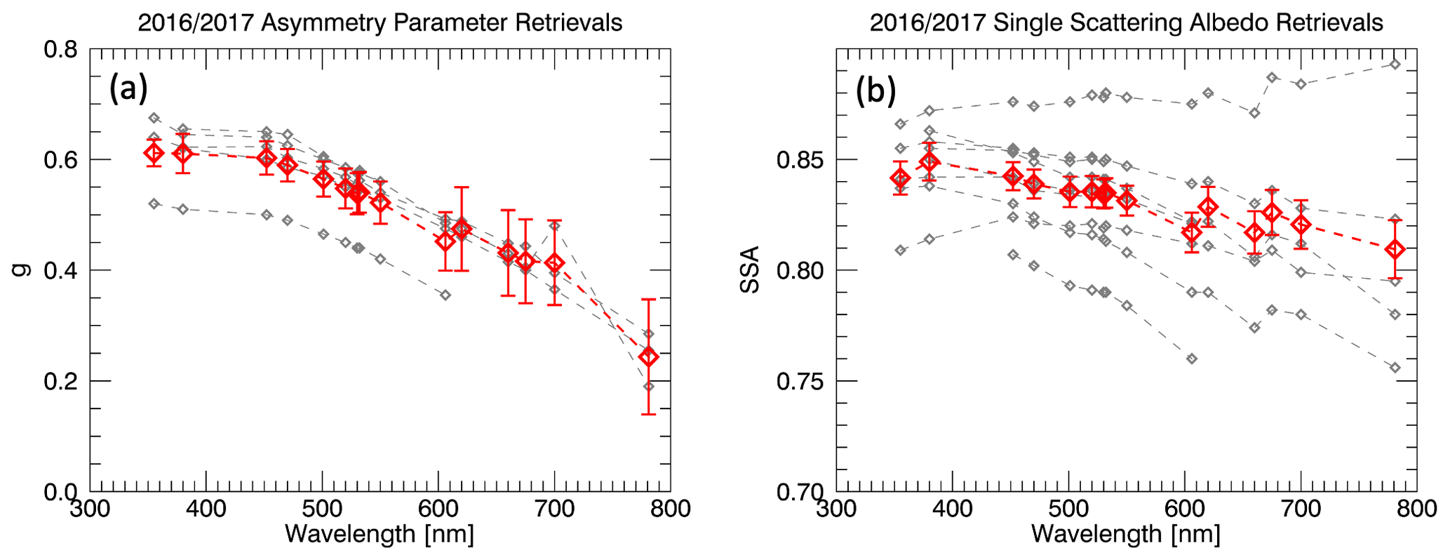
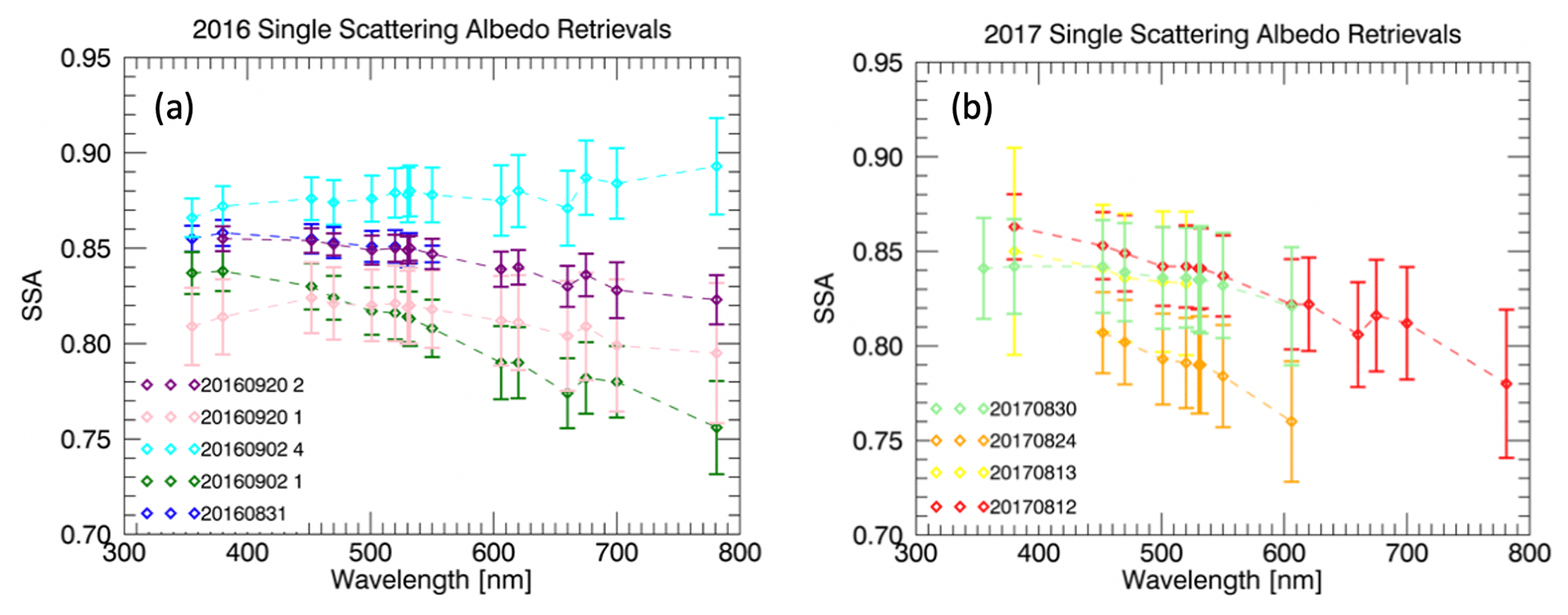
Figure 3Retrieved (a) asymmetry parameter and (b) SSA spectra for 2016 and 2017 successful retrievals. The red spectrum indicates the mean retrieved values with associated error bars; the grey spectra are the individual retrievals.
The asymmetry parameter decreases with increasing wavelength more rapidly than found in AERONET retrievals from sites in the southeast Atlantic (São Tomé, Ascension Island, and Namibia; Appendix B, Fig. B2). The AERONET retrieval algorithm is fundamentally different from the one used here. The AERONET operational inversion method assumes a size-independent complex refractive index (Dubovik and King, 2000), which can potentially lead to errors in the retrieved size distribution from which the optical properties are determined (Dubovik et al., 2002, 2006; Chowdhary et al., 2001). At 550 nm, the average g value is 0.52; by 660 nm, g has dropped to 0.43. Simple Mie calculations, shown in Appendix B, confirm that this spectral dependence is possible with a particular fine- to coarse-mode aerosol ratio. In addition, the AERONET sites are located at the perimeter of the ORACLES study region: at the very northern (São Tomé), western (Ascension), and southeastern (Namibia) ends of where the P-3 flew. As such, the aerosol measured at the AERONET sites might actually differ from that measured during our retrievals.
Table 3Mean retrieved SSA (row 3) and g (row 5) spectra along with their associated standard deviations (σ) (row 4 and row 6, respectively). The second row provides the number of valid retrievals for that wavelength. As described in C19, individual wavelengths can fail within the retrieval, resulting in fewer valid retrievals than valid cases (e.g., 355 nm SSA has five valid retrievals despite having nine valid cases).
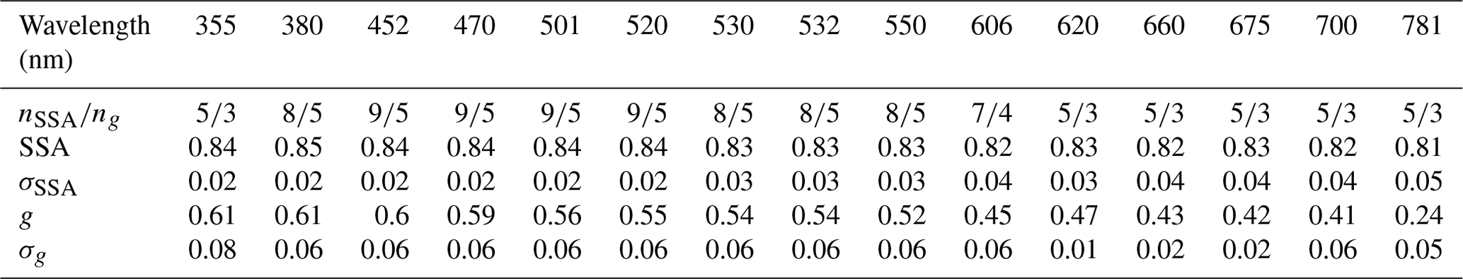
Figure 3b shows the retrieved SSA spectra from each successful spiral case, and the mean retrieved SSA and g for each wavelength are presented in Table 3. Our retrievals of SSA range from 0.78 to 0.88 at 550 nm, with an average value of 0.83. The red spectrum shows the mean of all cases. The SSA retrieved through our new method is spectrally flatter than reported from the SAFARI 2000 campaign, which took place in the southeastern region of the ORACLES measurement domain (Eck et al., 2003; Haywood et al., 2003; Russell et al., 2010). The SAFARI SSA values tend to be higher at the shorter wavelengths (i.e., < 550 nm), and they decrease more rapidly with increasing wavelength. The mean retrieved SSA values shown here are within the range of the 550 nm ORACLES 2016 SSA values from multiple instruments presented in Pistone et al. (2019) but are lower than most values from SAFARI 2000 (Haywood et al., 2003; Johnson et al., 2008; Russell et al., 2010). However, the mean SSA is close to the 0.85 value reported by Leahy et al. (2007). The lowest retrieved 550 nm SSA value is only slightly lower than that reported by Johnson et al. (2008) for the Dust and Biomass-burning Experiment (DABEX): 0.78 compared to 0.81.
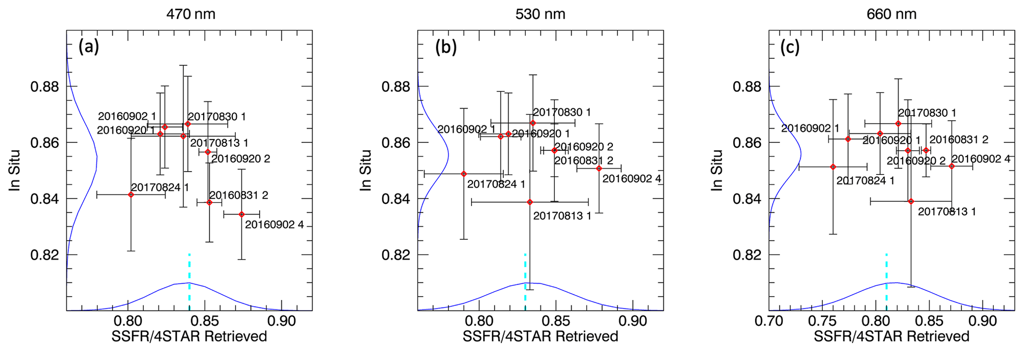
Figure 4In situ vs. retrieved SSA values for (a) 470, (b) 530, and (c) 660 nm. In situ values show transmittance-weighted SSA representative of the whole column, with error bars representing the standard deviation of all measured values throughout the spiral profile. In situ data are not available for the 20170812 case and are therefore not shown. The uncertainties for retrieved SSA for all wavelengths are provided in Appendix E. The blue dashed line indicates the values found by Davies et al. (2019).
Figure 4 compares our retrieved values of SSA to the in situ column average for (a) 450 nm, (b) 530 nm, and (c) 660 nm for all cases where such a comparison was possible. The in situ measurements are taken from a three-wavelength nephelometer (TSI 3563) and a three-wavelength particle soot absorption photometer (PSAP) (Radiance Research). The combination of scattering from the nephelometer and absorption from the PSAP provides SSA. SSA is calculated as the ratio of scattering from the nephelometer to the sum of scattering (again from the nephelometer) and absorption (from the PSAP). In order to best compare the retrieved values to the in situ values of SSA, the in situ measurements throughout the spiral profile are weighted by the weighting function, obtained by the transmittance, and then averaged to obtain a column value of SSA. Further details of the transmittance-weighted averaging can be found in Appendix C.
Although there are many factors that control aerosol SSA, such as emission state, source location, distance from the source, and age (Haywood et al., 2003; Eck et al., 2013; Konovalov et al., 2017; Dobracki et al., 2021), the values we find here are well within the range of SSA values reported by other ORACLES instruments (Pistone et al., 2019). As seen in Fig. 4, the mean SSFR/4STAR-retrieved SSA value tends to be slightly lower than the in situ mean (shown by the blue curve on the x and y axes). However, there does not seem to be a distinct correlation or anti-correlation for these cases, especially considering the uncertainties. This is consistent with the results shown in Pistone et al. (2019), which also showed no distinct correlation between the SSA derived or measured by different instruments (top row in Fig. 8).
It is important to note that the error bars shown in Fig. 4 reflect different values between the instruments: the in situ error bars represent the standard deviation of the entire column, whereas the SSFR-retrieved error bars represent the error estimate of the retrieval. The in situ measurements provide a range of SSA, and the standard deviation illustrates the variability throughout the aerosol layer. Conversely, the SSFR/4STAR retrieval provides only one value of SSA with the associated retrieval uncertainty for the entire layer. We cannot, however, detect any altitude dependence of SSA that may be present, such as suggested by Wu et al. (2020) and Dobracki et al. (2021).
In addition, new, more accurate (compared to filter-based in situ measurements), cavity ring-down and photoacoustic spectrometry instrumentation has recently been deployed to the southeast Atlantic during the CLARIFY-2017 deployment. Davies et al. (2019) performed an analysis of the SSA of aerosol dominated by biomass burning aerosol using such instrumentation and found mean SSA values of 0.84, 0.83, and 0.81 at interpolated wavelengths of 467, 528, and 652 nm, respectively. These values are included in Fig. 4 (dashed cyan line) to highlight the agreement with the results of this work. Wu et al. (2020) extended this analysis by examining the BBA in the free troposphere, finding a mean and variability in BBA SSA of 0.85 ± 0.02 and 0.82 ± 0.04 at 405 and 658 nm with evidence that the BBA at higher altitudes in the free troposphere is less absorbing. These results appear entirely consistent with those derived here.
3.2 DARE parameterizations
The first (basic) parameterization PDARE uses only two input parameters: AOD550 (mid-visible optical thickness) and α550 (scene or cloud albedo below the aerosol layer). The L and Q coefficients from Eq. (12) are derived from the nine individual cases (described in Sect. 3.3.1) where the corresponding fit coefficients for each of the cases are averaged to create the PDARE parameterization coefficients:
The coefficients l0, l1, l2, q0, q1, and q2 are the linear (l) and quadratic (q) coefficients of second-order polynomial fits to radiative transfer calculations for the DARE dependence on AOD550 of the individual cases as expressed in Eq. (12) for the average, which simultaneously capture the dependence on α550 as follows:
The overall PDARE coefficients are tabulated for each solar zenith angle SZA = {0, 5, …, 80∘} (see Table 4a).
Table 4(a) PDARE parameterization coefficients for differing SZAs. The collection of the coefficients represents the mean of all cases and the uncertainty values represent the standard deviation; the units on the L coefficients are W m−2/unit optical depth; the units on the Q coefficients are W m−2/(unit optical depth)2. (b) PXDARE additional coefficients for differing SZAs and their associated standard deviation, derived from the covariance matrix of the polynomial fits of Fig. 8a and b. These coefficients are used in Eqs. (22) and (23) (inserted into Eq. 24) and act as an extension to P in order to resolve the case-to-case variability resolvable through SSA. The units on the C1 and D1 coefficients are W m−2/unit optical depth; the units on the C2 and D2 coefficients are W m−2/(unit optical depth)2. The uncertainty columns represent the relative uncertainty of the delta correction terms. These uncertainties are applicable to Eqs. (22) and (23) and can be further propagated into Eq. (24).

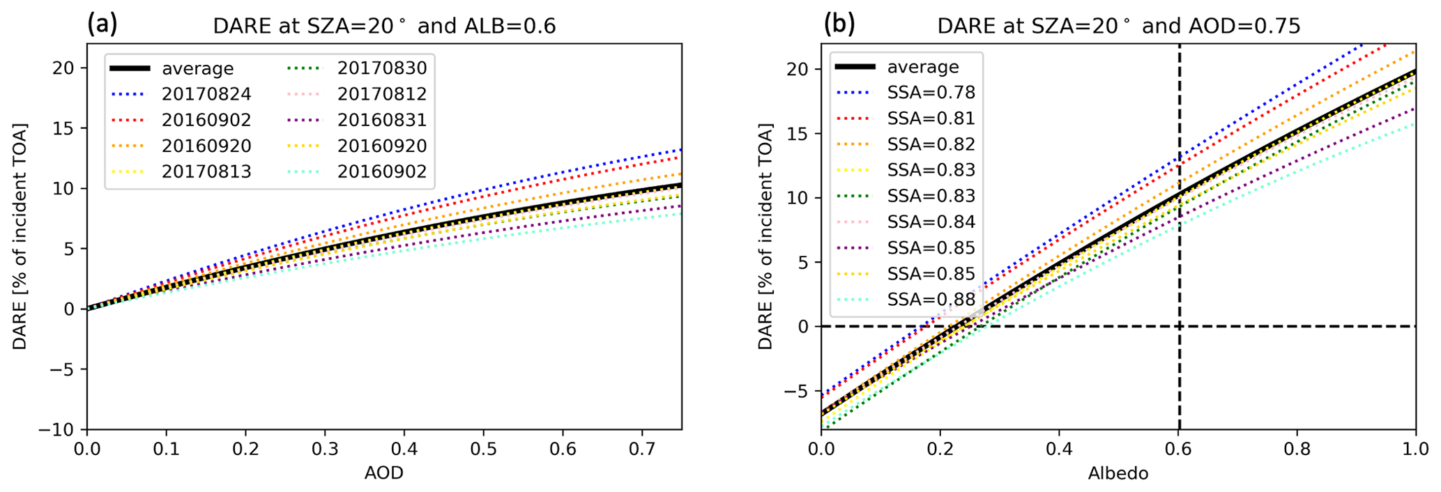
Figure 5(a) DARE as a function of AOD for fixed underlying albedo (0.6) and SZA (20∘), shown for the individual nine cases from this study (colors) and the average (black). The average is the basic parameterization result, PDARE. (b) DARE as a function of underlying albedo for a fixed AOD (0.75). The individual cases are labeled by their SSA at 550 nm (from more to less absorbing). The albedo at which the DARE changes is the critical albedo (horizontal dashed line). The vertical line marks an albedo of 0.6 for much of the ensuing discussion, which uses an AOD of 0.75, an albedo of 0.6, and a SZA of 20∘. It should be noted that a 20∘ SZA is not representative of the mean in the region.
Figure 5a shows the dependence of on the two input parameters for one specific SZA. DARE is shown in percent of top-of-atmosphere irradiance1, S0×cos (SZA), where S0=1365 W m−2. It is clearly nonlinear with respect to both input parameters, illustrating the need for a quadratic representation. However, the RFE from which PDARE originates is still encapsulated in this parameterization as
which is the slope of the black line at the origin in Fig. 5a. For an underlying albedo of 0, this reduces to RFE=L0. In this sense, the full parameterization PDARE generalizes RFE.
Whereas the black lines in Fig. 5a and b show the average ORACLES parameterization (i.e., PDARE) from Table 4a, the colored lines show the contributing nine cases, sorted by 550 nm SSA. It is apparent that the SSA introduces considerable case-to-case variability, especially for large albedos (Fig. 6), both in terms of the critical albedo (Fig. 7) and in terms of the magnitude of the DARE.
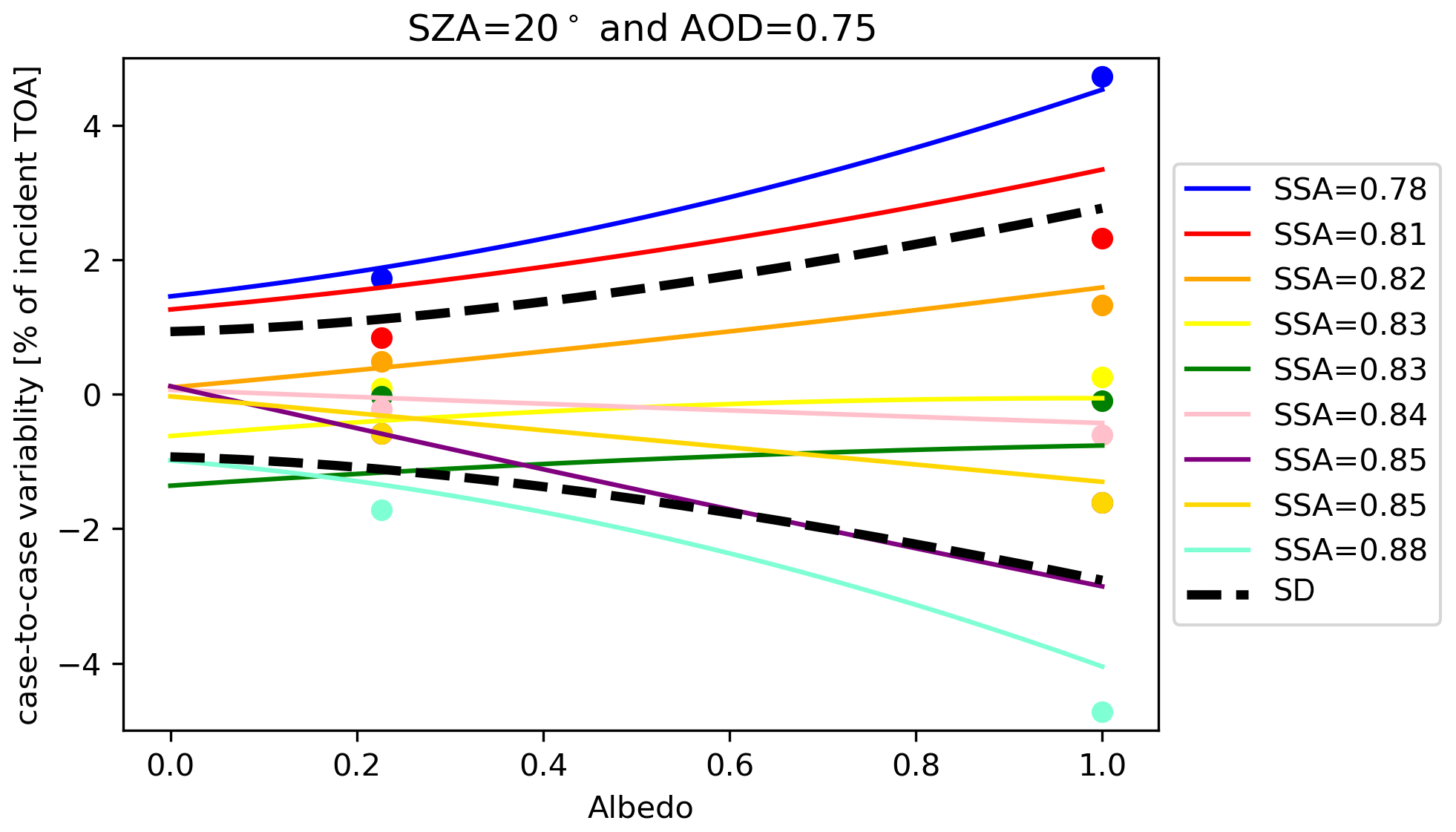
Figure 6The difference between PDARE and DARE for the individual cases at a fixed AOD (0.75) and SZA (20∘). The range of variability is represented by the standard deviation (black dashed curves).
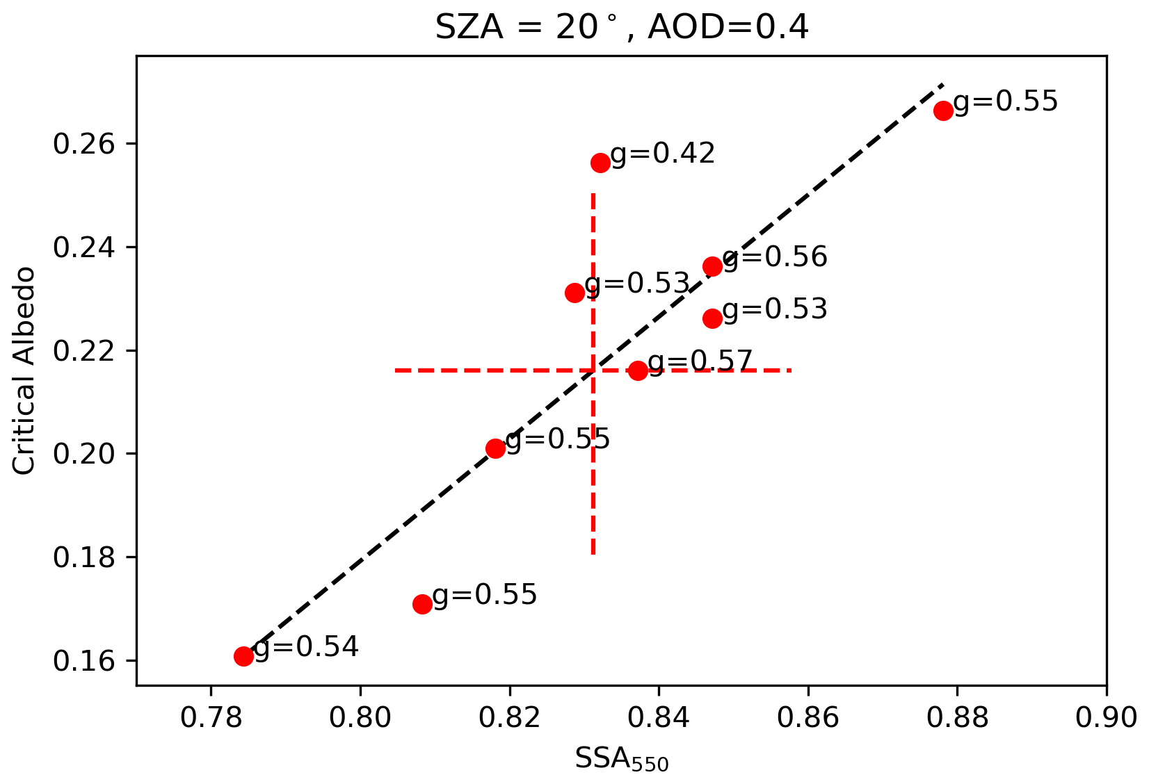
Figure 7Critical albedo as a function of mid-visible SSA. The red dashed cross shows the case-average αcrit.
Figure 6 shows the same as Fig. 5b, but here as the difference between the DARE for individual cases and PDARE (which represents the case-average DARE) expressed as a percentage difference in incident TOA solar flux. The ±σ range of variability (essentially the root mean square (rms difference, shown as dashed black lines in Fig. 7) is calculated from the standard deviation of this difference across all nine cases enumerated by c:
This serves as a metric for the case-to-case variability, which increases with the scene albedo and AOD. For example, the possible range in DARE for a mid-visible albedo of 0.6 and an AOD of 0.75 (SZA = 20∘) would be about 10 ± 2 % (or 136 ± 27 W m−2). This is without accounting for the uncertainty in the input parameters AOD and scene albedo, which have to be propagated through the parameterization via dP∕dAOD and dP∕dα. The uncertainty of 27 W m−2 in parentheses above can be interpreted as the uncertainty in DARE due to insufficient knowledge of SSA, which drives the case-to-case variability: in Figs. 5 and 6, the highest (lowest) SSA values correspond to the lowest (highest) DARE.
The extended parameterization PXDARE (Eq. 13) includes the SSA effect on DARE explicitly through an addition term not included in the PDARE parameterization (Eq. 12): .
In order to quantify the effect of SSA by this term, it is convenient to start with the dependence of the critical albedo on SSA (Fig. 7). To first approximation, this dependence can be represented by a linear fit. The critical albedo also weakly depends on the AOD and rather strongly on the SZA (not shown; for example, it can attain 0.6 at low Sun elevations) (Boucher et al., 1998). In contrast with the SSA, the asymmetry parameter does not drive the critical albedo in any discernible way, nor does it explain the deviation of the case-specific critical albedo from the fit line.
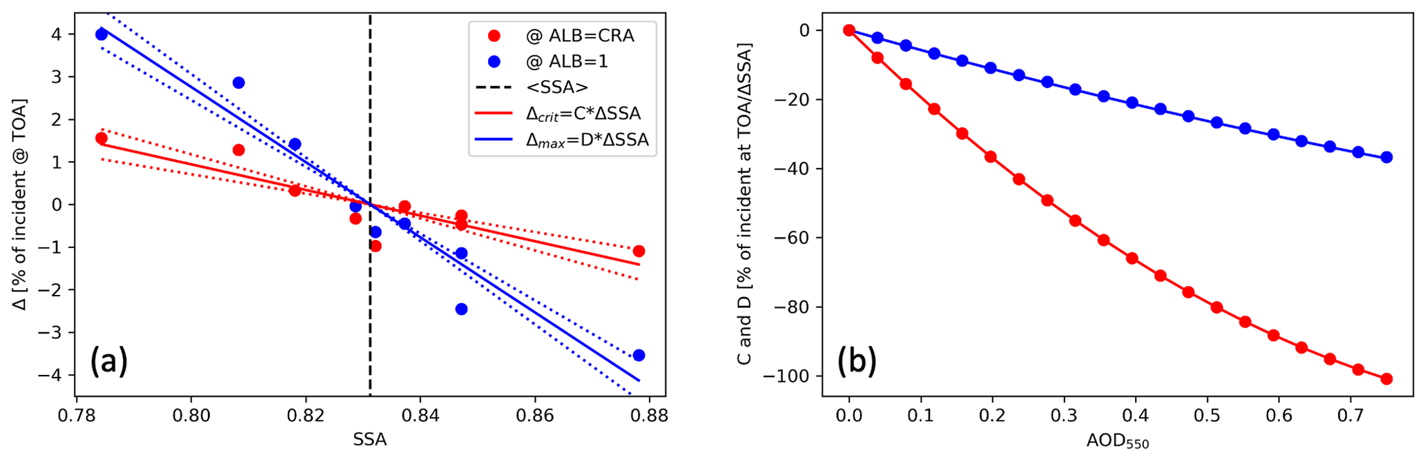
Figure 8(a) DARE perturbations as a function of SSA at the case-average critical albedo (red) and at albedo = 1 (blue) for SZA = 20∘. The vertical black dashed line indicates the case-average SSA. The dotted lines show the uncertainty in the C and D coefficients, which is propagated into the delta correction terms (Eqs. 22 and 23). (b) The dependence of the parameters C (red curve; determined at the critical albedo (Eq. 19) and D (blue curve; determined at albedo = 1 (Eq. 20) coefficients on mid-visible AOD.
In analogy to the SSA dependence of the critical albedo, the case-specific deviations of DARE from the case-average DARE (Fig. 6) can be represented as linear functions Δ(α,SSA) (Fig. 8a). Here, this is done by defining the DARE perturbation Δ(SSA) at two specific albedos: (1) at the case-average critical albedo (i.e., the albedo where DARE changes sign in Fig. 7) and (2) an albedo of 1 (maximum albedo):
where C and D are the slopes of the fit lines of Δ(αSSA) and ΔSSA is the difference between the case-specific SSA and the case-average SSA (, 0.83). The colored dots in Fig. 8a show Δcrit and Δmax, while Fig. 8b shows how the coefficients C and D depend on the AOD. This dependency can be represented as
where C1, C2, D1, and D2 (and the relative uncertainties for the Δcrit and Δmax terms) are tabulated in Table 4b for all solar zenith angles. Inserting Eqs. (20) into (18) and (21) into (19), the perturbations Δcrit and Δmax become
The perturbation at any albedo between the critical albedo and 1 is simply calculated as
while Δ(α)=Δcrit for α < αcrit.
Equations (21), (22), (23), and (24) are used collectively to determine the additional term for the PXDARE parameterization (Eq. 13).
If SSA is known in addition to AOD and scene albedo, then PXDARE captures DARE to greater fidelity than does PDARE. This is shown by the case-to-case variability in Fig. 9, expressed as the difference between the DARE for the individual cases in analogy to Fig. 6. The ±σ range of variability in Fig. 9 is much smaller than that in Fig. 6, showing that the uncertainty in PXDARE (±0.5 % at an albedo of 0.3 of the incident irradiance at TOA) is significantly below the unresolved variability in PDARE due to an unknown SSA (±1.2 % at an albedo of 0.3, up to 2 % at an SZA of 20∘).

Figure 9The difference between PXDARE and PDARE for nine case SSAs at fixed AOD (0.75) and SZA (20∘).
Beyond the case-to-case variability, Fig. 10 confirms that including the SSA information in PXDARE does in fact reproduce DARE well for each individual case, as illustrated by the agreement between the solid (PXDARE) and individual case RTM-calculated DARE. The residuals between the direct RTM DARE output and DARE estimated using PDARE and PXDARE (shown as contours in Fig. 11a and b) provide an estimate of the overall uncertainties inherent within the parameterizations.
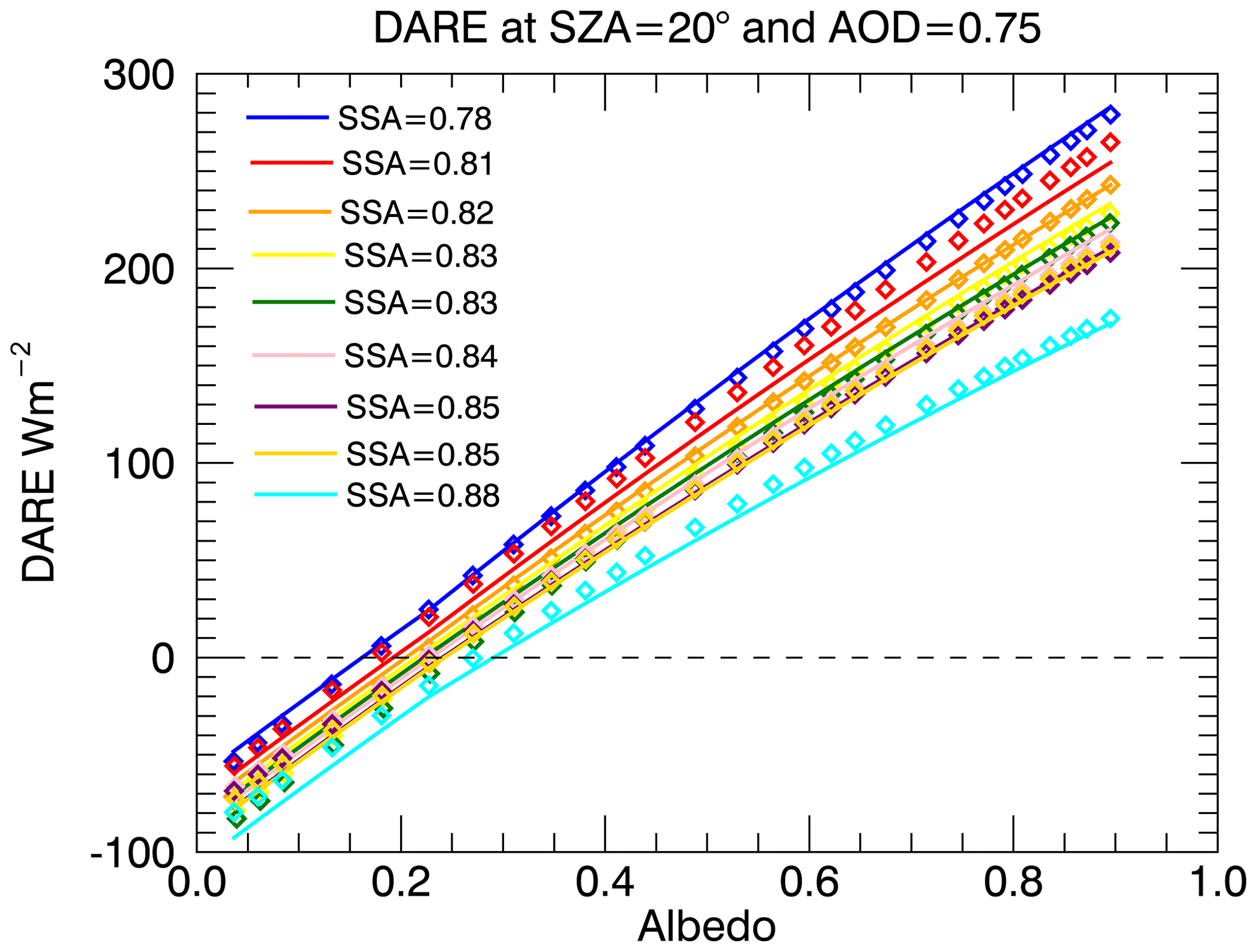
Figure 10DARE as predicted by PXDARE for the nine cases (solid lines) and DARE as calculated by the RTM (dotted colored lines).
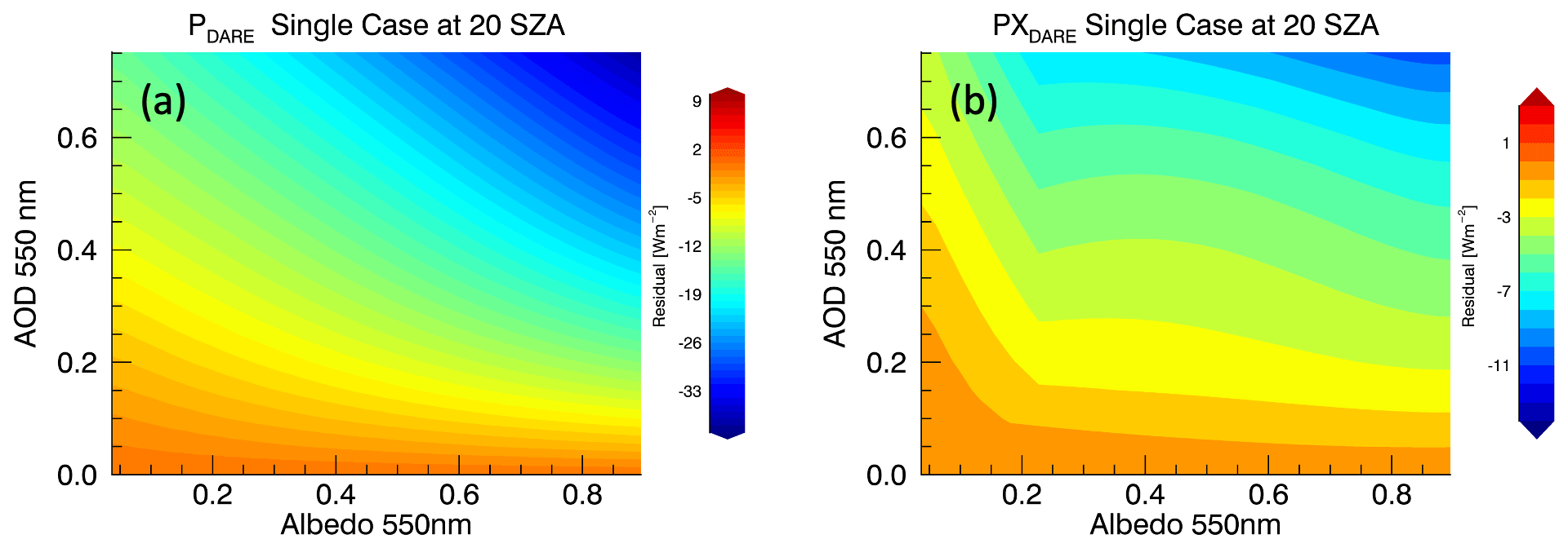
Figure 11Residual plot of directly calculated DARE (RTM output) and predicted BB DARE values using (a) PDARE and (b) PXDARE for a single case at a fixed SZA (20∘). Residual plots for each case can be found in Appendix D. For both figures, the residuals encompass the difference between the RTM and the PDARE and PXDARE parameterizations.
As Fig. 11a shows, the residuals of PXDARE are significantly smaller than those of PDARE. Both PDARE and PXDARE have small uncertainty contributions from a number of factors (e.g., measurement uncertainty of SSFR, RTM uncertainty, conversion and extrapolation from spectrally resolved retrievals to broadband values, the uncertainty of the quadratic fit leading to the L and Q coefficients, and the uncertainty in the fits leading to the C and D coefficients), but PDARE also encompasses the variability due to SSA which leads to a much larger uncertainty in PDARE than PXDARE.
In this paper, we systematically linked aircraft observations of spectral fluxes to aerosol optical thickness and other parameters, using nine cases from the 2016 and 2017 ORACLES campaigns. This observationally driven link is expressed by two parameterizations of the shortwave broadband DARE, (1) in terms of the mid-visible AOD and scene albedo (PDARE) and (2) in terms of the mid-visible AOD, scene albedo, and aerosol SSA (PXDARE). These parameterizations can be used to translate from AOD and scene albedo (optionally also from SSA) to DARE directly, bypassing radiative transfer calculations that are usually required to arrive at DARE from observations. This is advantageous when satellite retrievals provide only limited information such as AOD and scene albedo (by way of cloud fraction and optical thickness), but not aerosol microphysics, hygroscopic growth, or optical properties. However, this parameterization only captures the natural variability of the study region as sampled. It therefore does not necessarily represent the entire southeast Atlantic, let alone during times beyond the ORACLES campaigns. Despite this caveat, one could interpret the parameterization as the start of a DARE climatology built on two (or three) driver variables. Additional observations extending the statistics to other regions and time periods could easily be added to this framework. For example, the 2018 ORACLES data will be incorporated in a separate paper.
We find that the two parameterizations reproduce the case-specific DARE to different degrees. The majority of the case-to-case variability within the ORACLES DARE dataset is attributable to the dependence on AOD and scene albedo. Using just these two variables to span the first parameterization, PDARE, the rms bias of the case-specific DARE with respect to the parameterized baseline is 1 %–2 % of the incident radiation for an SZA of 20∘ and an AOD of 0.75 (Fig. 6), with a DARE value of 10 % of the incident radiation for a scene albedo of 0.6 (Fig. 5b). Translated into flux units, the DARE for this constellation of scene parameters is 136 ± 27 W m−2, where the range of uncertainty stems from the unexplained case-to-case variability as obtained from the rms bias. In other words, this parameterization leads to 20 % DARE uncertainty due to the variability of the system caused by factors other than AOD and scene albedo. If satellites only provided AOD and scene albedo, this would be the uncertainty of the derived DARE (leaving the retrieval uncertainties of AOD and albedo aside for the moment). In reality, the variability is likely even larger than captured with our limited samples, so this estimate is a lower bound on the DARE variability.
Fortunately, our research showed that we can actually explain more of the case-to-case variability by introducing the mid-visible SSA as a third parameter in an extended parameterization PXDARE. This reduces the variability by a factor of 4 by explicitly resolving the case-to-case variability via SSA: a DARE value of 136 ± 6.8 W m−2 corresponds to an SSA of 0.83 (campaign average at 550 nm), whereas 0.81 (typical low SSA value encountered during ORACLES) yields a DARE of 177 ± 10.6 W m−2. The remaining uncertainty (about 5 %) is due to variability drivers beyond AOD, scene albedo, and SSA, such as variable aerosol microphysics or hygroscopicity. It also encompasses the measurement uncertainty of SSFR and 4STAR.
Interestingly, the mid-visible asymmetry parameter (also retrieved for most cases) is not a significant driver of the case-to-case variability. However, the retrieved spectra of SSA and asymmetry parameter can be useful for future satellite retrievals of cloud and aerosol optical thickness in the study region. Since these retrievals are directly tied to the radiative fluxes, they work without assumptions about the scattering phase function, size distribution, or aerosol type, nor do they require smoothness constraints. However, an optical closure study that involves in situ measurements of aerosol microphysics and optical properties in conjunction with Mie calculations is required before our results can be of practical use, especially at wavelengths beyond the visible range where our retrieval uncertainties grow large. Our asymmetry parameter spectra fall off faster with wavelength than usually assumed based on land-based observations, which may be an indication that there is less coarse mode in the ORACLES measurements, which are almost exclusively over ocean.
We cannot judge whether our approach will be useful for predictive models, which usually follow the “bottom-up” paradigm; i.e., they arrive at DARE starting from detailed aerosol and cloud properties via radiative transfer calculations. At the very least, the agreement between the absolute values and spectral dependence of the SSA and asymmetry parameter retrievals coming out of our and other ORACLES/LASIC/CLARIFY-2017/AEROCLO-Sa studies (Zuidema et al., 2016) such as Davies et al. (2019) and Wu et al. (2020) will provide robust constraints of the aerosol optical properties in a range of models. However, we also anticipate that our parameterized, observationally based DARE could serve as a simple, built-in closure for the calculated DARE, adding a “top-down” model constraint, or even prove useful for model tuning.
Our paper is focused on instantaneous DARE and stops short of providing an “all-ORACLES” (diurnally integrated) DARE estimate. A promising approach in this regard is to use geostationary satellite retrievals of cloud and aerosol properties (Peers et al., 2020) in conjunction with in situ aircraft data and radiative transfer calculations. Alternatively, one can use the satellite radiances to extrapolate from the spatially and temporally limited aircraft observations to obtain regional estimates of the diurnally integrated DARE, circumventing the satellite retrievals. This approach, already underway within our group, builds on the P or PX parameterization, specifically by using albedo data from the geostationary Spinning Enhanced Visible and Infrared Imager (SEVIRI) in combination with ORACLES AOD data from HSRL-2 and 4STAR. A grid-box-specific model-to-observation inter-comparison is also underway in the wider ORACLES team. While we limited this paper to the above-layer (TOA) DARE, the radiative effect of aerosols on the layer itself (i.e., the heating rate) is also an important deliverable from ORACLES, which will be presented in a separate follow-up paper.
Making the transition from the spectral to broadband is one of the main hurdles for both the parameterizations presented in this paper and for broadband DARE studies in general. Broadband DARE calculations require accurate aerosol and cloud information for all wavelengths, and it can be difficult to accurately determine the correct spectral dependence of these properties. The cloud albedo is particularly challenging since the spectral dependence depends on the SZA.
In our work, the aerosol optical properties of SSA and g can be retrieved for wavelengths up to 781 nm, and AOD values from 4STAR can be retrieved for up to 1650 nm. Cloud albedo is measured for the entire SSFR wavelength range, but only for a single SZA value (the mean SZA throughout the spiral time period). We therefore must (a) interpolate between wavelengths and (b) extend each optical property to longer wavelengths to the best of our knowledge and compute the cloud albedo for a range of SZAs.
A1 SSA
To extend the retrieved SSA values to the remaining reported 4STAR wavelengths, we rely on the AAOD, defined as
First, we calculate a fit line in log–log space of the AAOD for wavelengths where we have valid SSFR SSA retrievals. We extend that fit to obtain the AAOD for the remaining 4STAR wavelengths. We then re-arrange Eq. (A1) to determine SSA for those wavelengths where we do not have SSFR SSA retrievals. Finally, we set the SSA at wavelengths longer than 1650 nm to the mean of the longest 4STAR wavelengths, 1600 and 1650 nm. A1a illustrates the extension of SSA.
A2 Asymmetry parameter
Using the SSFR-retrieved g values, we calculate a polynomial fit for the available wavelengths. We then extend the fit to longer wavelengths. Once the fit reaches 0, the remaining wavelengths are set to 0. While it would have been possible to instead use the fine-mode Mie calculations (Fig. B1), we chose to utilize the retrievals and approximate the fine mode, jumping to zero lacking other information. An optical closure study, though beyond the scope of this paper, is necessary. Figure A1b illustrates the extension of g.
A3 Developing the parameterization grid
In order to calculate the parameterization, we grid the AOD and albedo spectra, preserving the specific spectral shapes.
A3.1 AOD
We take the measured AOD spectrum at the BOL and multiply that spectrum by a factor to create a grid such that the values at 550 nm range from 0 to 0.75. In this way, each case has a normalized AOD grid at 550 nm while maintaining the specific spectral shape of the measured spectrum. We then extrapolate the AOD spectra to the remaining wavelengths. Figure A1c illustrates the extension and gridding of AOD.
A3.2 Albedo
Obtaining the cloud albedo requires the RTM to be used to maintain accurate representation of the spectral shape. First, we retrieve the cloud properties of effective radius (Reff) and cloud optical thickness (COT) from the measured albedo using the RTM, with retrieval wavelengths of 1200 and 1630 nm. We then grid COT from 0 to 100 while keeping Reff constant at the retrieved value. We run the RTM to calculate a spectral albedo grid for all new pairs of Reff and COT for the range of SZAs. In these calculations, the surface for the cloud retrievals is standard Lambertian with an albedo value of 0.03. The COT range begins at 0, and this translates to a 0 “surface” albedo for the parameterization. It is acknowledged that clouds do not exhibit a Lambertian albedo. However, for irradiance calculations, the cloud albedo (non-Lambertian) can be substituted with a Lambertian albedo. Also, it is acknowledged that a sea surface is even less of a Lambertian reflector than a cloud. However, this is precisely the simplification that we made to fit both cloudy and cloud-free skies into a common framework. Since we are interested in DARE (the difference of fluxes) rather than the fluxes themselves, these simplifications should lead to only negligible effects relative to the contributing measurement uncertainties. Figure A1d illustrates the albedo grid for a single SZA.
While we extend the aerosol and cloud properties as accurately as possible, it is most crucial that the shortest wavelengths are accurate. At the longer wavelengths, the AOD becomes increasingly small, and the optical property accuracy is therefore less critical. This works in our favor since the SSFR retrieval is valid for this wavelength range where the AOD and absorption are large.
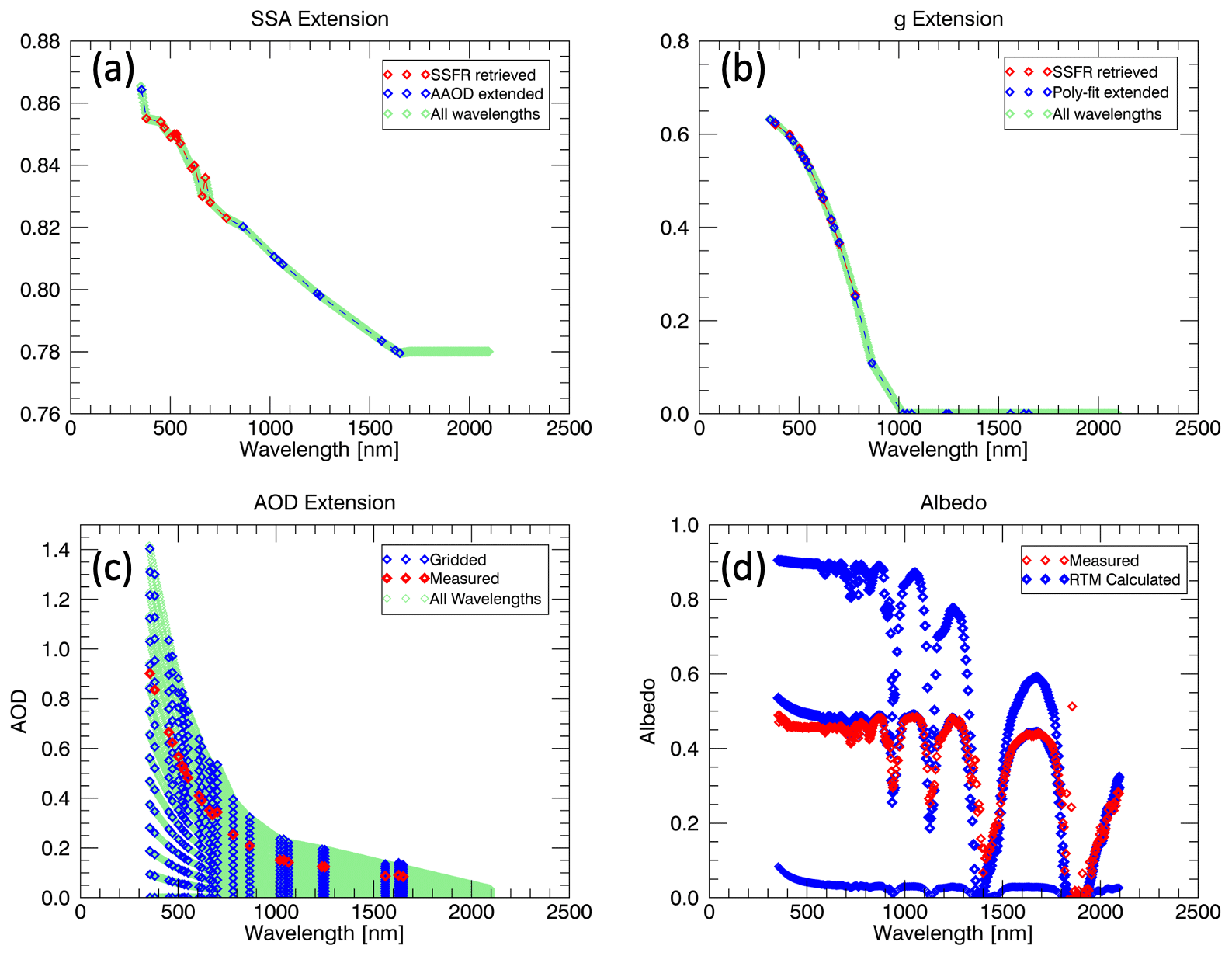
Figure A1One example case of the extension of aerosol properties to longer wavelengths for (a) SSA, (b) g, and (c) AOD. Panel (d) shows the SSFR-measured vs. RT-calculated albedo spectra along with the RT-calculated spectra for 0 COT and 100 COT.
The SSFR spectral irradiance aerosol retrieval is fundamentally different than most other aerosol retrievals, which are rooted in knowledge of the aerosol size distribution along with both the imaginary and real parts of the index of refraction. These methods must utilize Mie calculations to get to the aerosol optical properties of SSA and g. As described in Pistone et al. (2019), ORACLES instrumentation such as 4STAR, the Research Scanning Polarimeter (RSP), and the Airborne Multi-angle SpectroPolarimeter Imager (AirMSPI) utilize this technique to obtain aerosol properties. The SSFR retrieval, on the other hand, circumvents the need for Mie calculations and knowledge of the size distribution or index of refraction by relying on the measured aerosol absorption itself.
However, simple Mie calculations (Fig. B1) verify that a quickly decreasing asymmetry parameter is possible, and it will even decrease to 0 if no coarse mode is present. However, that is unlikely. It is more likely that the asymmetry parameter will eventually go back up again for long wavelengths – a result of even small coarse-mode concentrations.
Beyond the ORACLES-specific instrumentation, AERONET stations across the globe utilize sunphotometers with the same underlying retrieval algorithms as used with 4STAR sky radiances to provide aerosol optical properties. In Fig. B2a and b, we show the mean SSFR SSA and g retrieval spectra compared to the nearest AERONET sites for 2016 and 2017: São Tomé, Ascension, and Namibia.
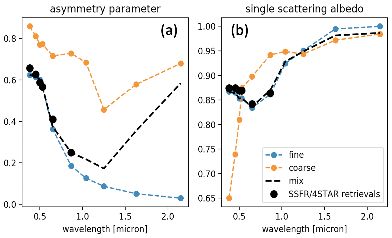
Figure B1Mie calculations of (a) g and (b) SSA compared to SSFR/4STAR-retrieved values. The black dots show the asymmetry parameter spectrum (left) and SSA spectrum (right) as retrieved from SSFR/4STAR; the blue dot-dash line shows a fine-mode aerosol (r = 0.13 nm) with a real index of refraction of 1.6 and an imaginary index of refraction ranging from 0.05 (380 nm) to 0 (2 nm); the orange dot-dash line shows a coarse-mode aerosol (r = 1.3 nm) with the real index of refraction of 1.6 and an imaginary index of refraction ranging from 0.015 (380 nm) to 0.003 (600 nm) (Wagner et al., 2012). The black line shows a mix of coarse/fine aerosol (0.02 : 2 optical thickness ratio).
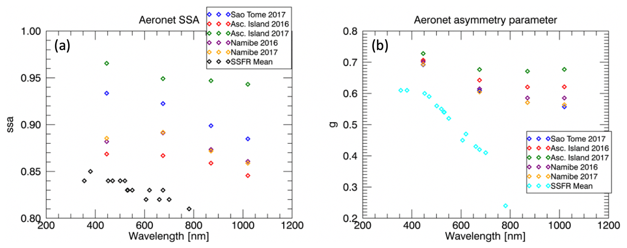
Figure B2Retrieved values of (a) SSA and (b) g compared AERONET-measured values at nearby land sites.
In situ SSA measurements and SSFR SSA retrievals cannot be compared directly since in situ SSA measurements are made continuously throughout the column (spiral), across variations in aerosol concentrations, whereas the SSFR SSA values represent a single value representative of the entire column. In order to best compare the in situ and retrieved SSA values, we calculate a weighted in situ SSA average, using a weighting function based on the transmittance through the aerosol layer.
In past studies (e.g., C19; Pistone et al., 2019), the in situ SSA measurements were averaged with each SSA value weighted by its corresponding measured extinction, which better represents the column SSA than a simple average. However, it is the transmittance rather than the extinction which describes the aerosols' impact on the radiation throughout the layer. Since the SSFR SSA retrieval is based on the change in radiation through the aerosol layer, it is most consistent to weigh the in situ measurements on transmittance rather than extinction.
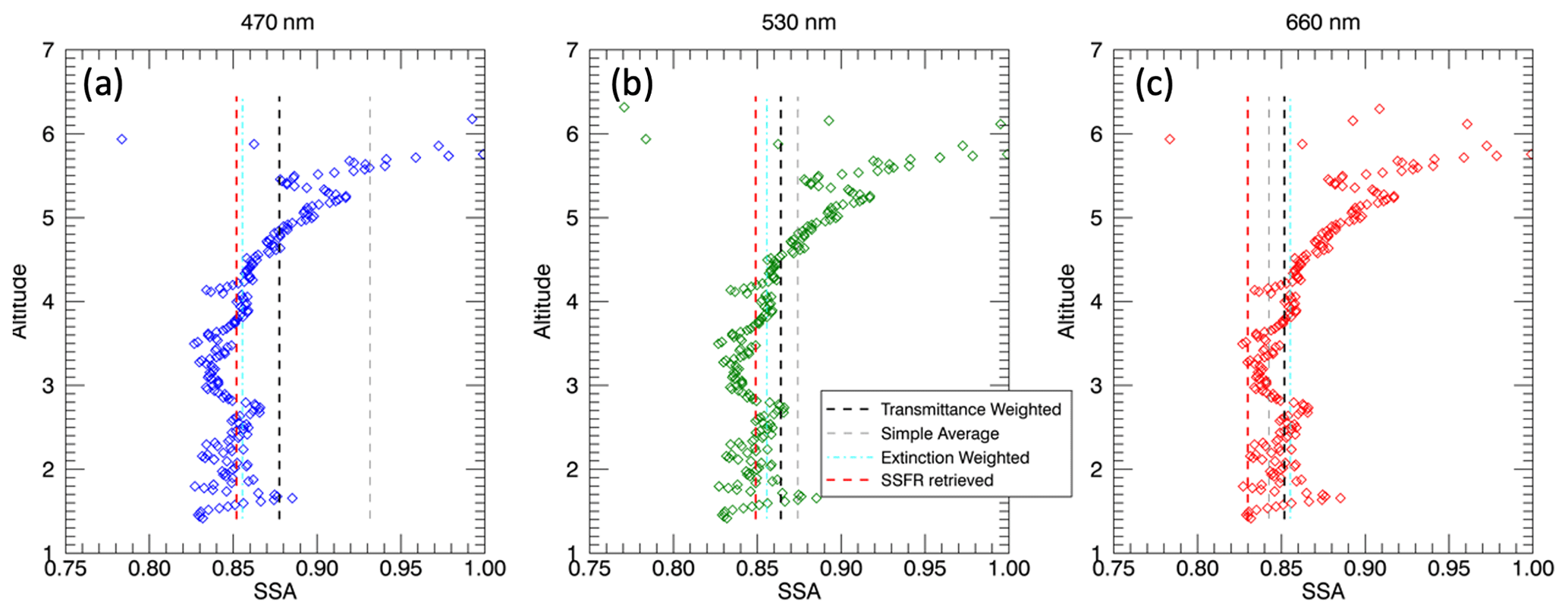
Figure C1An example of one spiral case with the different in situ averages along with the SSFR-retrieved SSA for (a) 450 nm, (b) 530 nm, and (c) 660 nm. The colored points show the in situ data as measured throughout the profile.
For each spiral profile, we take the extinction profile as measured by the in situ instruments to calculate the weighting function as follows:
where βe(z) is the extinction, t(z) is the transmittance, and .
Figure C1 shows the in situ measured SSA profile for one profile case at (a) 470 nm, (b) 530 nm, and (c) 660 nm. The red dashed line shows the SSFR/4STAR-retrieved value; the black dashed line shows the transmittance-weighted in situ SSA value; the grey dashed line shows the extinction-weighted in situ SSA value.
Figures D1 and D2 show the residual values between directly calculated DARE (by the RTM) and DARE calculated using (D1) PDARE and (D2) PXDARE for each case. The residuals are significantly higher when using PDARE vs. PXDARE, illustrating that including the additional constraint of SSA (i.e., PXDARE) greatly improves the parameterization performance.
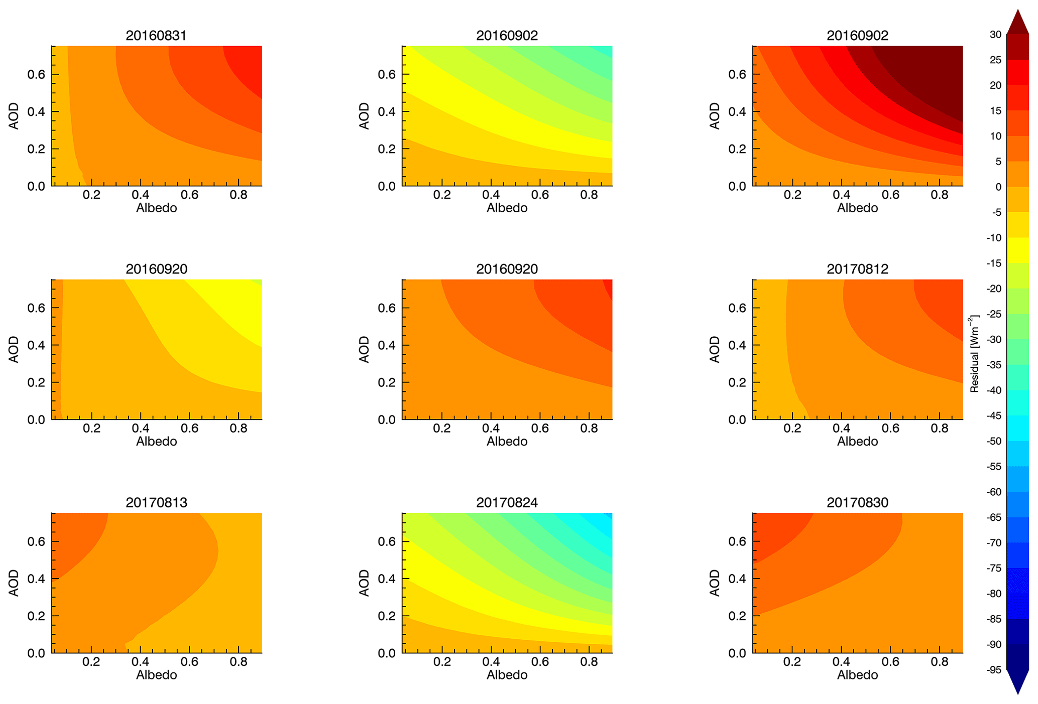
Figure D1Residual plot of directly calculated DARE (RTM output) and predicted BB DARE values using PDARE at a fixed SZA (20∘).

Figure D2Residual plots of directly calculated DARE (RTM output) and predicted broadband DARE values using PXDARE at a fixed SZA (20∘).
Retrievals of SSA for each individual case with the associated retrieval uncertainty are shown as error bars. Figure E1 shows the SSA retrievals for (a) 2016 and (b) 2017.
The 2016 and 2017 ORACLES data are publicly available at https://doi.org/10.5067/Suborbital/ORACLES/P3/2016_V1 (ORACLES Science Team, 2017) and https://doi.org/10.5067/Suborbital/ORACLES/P3/2017_V1 (ORACLES Science Team, 2019). The parameterization coefficients and accompanying code are publicly available at https://doi.org/10.5281/zenodo.4311591 (Cochrane and Schmidt, 2020).
SPC collected SSFR data, performed the bulk of the analysis, and wrote the majority of the paper with input from the other authors. KSS collected SSFR data, helped with the methodology development and data analysis, and helped with developing, writing, and editing the paper. HC, PP, and SK helped with the data collection of SSFR. JR was one of the PIs for the ORACLES campaign and provided 4STAR data. SL was the PI of the 4STAR instrument and helped with the retrieval methodology. KP, MK, MSR, YS, and CF provided 4STAR data. SH, SF, and AD provided in situ data. PZ and SD were on the leadership team for the ORACLES project and helped advise data use. All the co-authors helped in the reviewing and editing of the paper.
The authors declare that they have no conflict of interest.
This article is part of the special issue “New observations and related modelling studies of the aerosol–cloud–climate system in the Southeast Atlantic and southern Africa regions (ACP/AMT inter-journal SI)”. It is not associated with a conference.
This work was supported by NASA grant NNX15AF62G. We thank the ORACLES deployment support teams and the science team for a successful and productive mission. We thank Warren Gore of NASA AMES for his support during the ORACLES mission. Thank you to each of the instrument teams who provided data and expertise on using them.
This research has been supported by NASA (grant no. NNX15AF62G).
This paper was edited by Piet Stammes and reviewed by Jim Haywood and one anonymous referee.
Anderson, G. P., Shepard, A. C., Kneizys, F. X., James, Chetwynd, H., and Eric, P. S.: AFGL atmospheric constituent profiles (0.120 km), Report No. AFGL-TR-86-0110, Air Force Geophysics Lab Hanscom AFB MA, 1986.
Boucher, O., Schwartz, S. E., Ackerman, T. P., Anderson, T. L., Bergstrom, B., Bonnel, B., Chylek, P., Dahlback, A., Fouquart, Y., Fu, Q., Halthore, R. N., Haywood, J. M., Iversen, T., Kato, S., Kinne, S., Kirkevag, A., Knapp, K. R., Lacis, A., Laszlo, I., Mishchenko, M. I., Nemesure, S., Ramaswamy, V., Roberts, D. L., Russell, P., Schlesinger, M. E., Stephens, G. L., Wagener, R., Wang, M., Wong, J., and Yang, F.: Intercomparison of models representing direct shortwave radiative forcing by sulfate aerosols, J. Geophys. Res.-Atmos., 103, 16979–16998, 1998.
Chand, D., Wood, R., Anderson, T. L., Satheesh, S. K., and Charlson, R. J.: Satellite-derived direct radiative effect of aerosols dependent on cloud cover, Nat. Geosci., 2, 181–184, 2009.
Chowdhary, J., Cairns, B., Mishchenko, M., and Travis, L.: Retrieval of aerosol properties over the ocean using multispectral and multiangle photopolarimetric measurements from the Research Scanning Polarimeter, Geophys. Res. Lett., 28, 243–246, https://doi.org/10.1029/2000GL011783, 2001.
Coakley, J. A. and Chylek, P.: The two-stream approximation in radiative transfer: Including the angle of the incident radiation, J. Atmos. Sci., 32, 409–418, https://doi.org/10.1175/1520-0469(1975)032<0409:TTSAIR>2.0.CO;2, 1975.
Cochrane, S. and Schmidt, K. S.: Parameterization Coefficients for AMT article: Empirically-Derived Parameterizations of the Direct Aerosol Radiative Effect based on ORACLES Aircraft Observations, Zenodo, https://doi.org/10.5281/zenodo.4311591, 2020.
Cochrane, S. P., Schmidt, K. S., Chen, H., Pilewskie, P., Kittelman, S., Redemann, J., LeBlanc, S., Pistone, K., Kacenelenbogen, M., Segal Rozenhaimer, M., Shinozuka, Y., Flynn, C., Platnick, S., Meyer, K., Ferrare, R., Burton, S., Hostetler, C., Howell, S., Freitag, S., Dobracki, A., and Doherty, S.: Above-cloud aerosol radiative effects based on ORACLES 2016 and ORACLES 2017 aircraft experiments, Atmos. Meas. Tech., 12, 6505–6528, https://doi.org/10.5194/amt-12-6505-2019, 2019.
Davies, N. W., Fox, C., Szpek, K., Cotterell, M. I., Taylor, J. W., Allan, J. D., Williams, P. I., Trembath, J., Haywood, J. M., and Langridge, J. M.: Evaluating biases in filter-based aerosol absorption measurements using photoacoustic spectroscopy, Atmos. Meas. Tech., 12, 3417–3434, https://doi.org/10.5194/amt-12-3417-2019, 2019.
Dobracki, A., Zuidema, P., Howell, S., Saide, P., Freitag, S., Aiken, A., Coe, H., Podolske, J., Sedlacek, A., Redemann, J., Taylor, J., Thornhill, L., Wood, R., and Wu, H.: Understanding the Lifetime of Observed Biomass Burning Aerosol in the Free Troposphere, American Meteorological Society Annual Meeting, 10–15 January 2021, New Orleans, Louisiana, USA, 2021.
Dubovik, O. and King, M. D.: A flexible inversion algorithm for retrieval of aerosol optical properties from Sun and sky radiance measurements, J. Geophys. Res., 105, 20673–20696, 2000.
Dubovik, O., Holben, B. N., Eck, T. F., Smirnov, A., Kaufman, Y. J., King, M. D., Tanré, D., and Slutsker, I.: Variability of absorption and optical properties of key aerosol types observed in worldwide locations, J. Atmos. Sci., 59, 590–608, https://doi.org/10.1175/1520-0469(2002)059<0590:VOAAOP>2.0.CO;2, 2002.
Dubovik, O., Sinyuk, A., Lapyonok, T., Holben, B. N., Mishchenko, M., Yang, P., Eck, T. F., Volten, H., Munoz, O., Veihelmann, B., van der Zande, W. J., Leon, J.-F., Sorokin, M., and Slutsker, I.: Application of spheroid models to account for aerosol particle nonsphericity in remote sensing of desert dust, J. Geophys. Res., 111, D11208, https://doi.org/10.1029/2005JD006619, 2006.
Dunagan, S., Johnson, R., Zavaleta, J., Russell, P., Schmid, B., Flynn, C., Redemann, J., Shinozuka, Y., Livingston, J., and Segal Rozenhaimer, M.: Spectrometer for Sky-Scanning Sun-Tracking Atmospheric Research (4STAR): Instrument Technology, Remote Sens., 5. 3872–3895, https://doi.org/10.3390/rs5083872, 2013.
Eck, T. F., Holben, B. N., Ward, D. E., Mukelabai, M. M., Dubovik, O., Smirnov, A., Schafer, J. S., Hsu, N. C., Piketh, S. J., Queface, A., Le Roux, J., and Slutsker, I.: Variability of biomass burning aerosol optical characteristics in southern Africa during the SAFARI 2000 dry season campaign and a comparison of single scattering albedo estimates from radiometric measurements, J. Geophys. Res., 108, 8477, https://doi.org/10.1029/2002JD002321, 2003.
Eck, T. F., Holben, B. N., Reid, J. S., Mukelabai, M. M., Piketh, S. J., Torres, O., Jethva, H. T., Hyer, E. J., Ward, D. E., Dubovik, O., Sinyuk, A., Schafer, J. S., Giles, D. M., Sorokin, M., Smirnov, A., and Slutsker, I.: A seasonal trend of single scattering albedo in southern African biomass-burning particles: Implications for satellite products and estimates of emissions for the world's largest biomass-burning source, J. Geophys. Res., 118, 6414–6432, https://doi.org/10.1002/jgrd.50500, 2013.
Emde, C., Buras-Schnell, R., Kylling, A., Mayer, B., Gasteiger, J., Hamann, U., Kylling, J., Richter, B., Pause, C., Dowling, T., and Bugliaro, L.: The libRadtran software package for radiative transfer calculations (version 2.0.1), Geosci. Model Dev., 9, 1647–1672, https://doi.org/10.5194/gmd-9-1647-2016, 2016.
Forster, P., Ramaswamy, V., Artaxo, P., Berntsen, T., Betts, R., Fahey, D. W., aywood, J., Lean, J., Lowe, D. C., Myhre, G., Nganga, J., Prinn, R., Raga, G., Schulz, M., and Van Dorland, R.: Changes in Atmospheric Constituents and in Radiative Forcing, in: Climate Change 2007: The Physical Science Basis, Contribution of Working Group I to the Fourth Assessment Report of the Intergovernmental Panel on Climate Change, edited by: Solomon, S., Qin, D., Manning, M., Chen, Z., Marquis, M., Averyt, K. B., Tignor, M., and Miller, H. L., Cambridge University Press, Cambridge, United Kingdom and New York, NY, USA, 2007.
Hansen, J., Sato, M., and Ruedy, R.: Radiative forcing and climate response, J. Geophys. Res., 102, 6831–6864, https://doi.org/10.1029/96JD03436, 1997.
Haywood, J. M. and Shine, K. P.: The effect of anthropogenic sulfate and soot aerosol on the clear sky planetary radiation budget, Geophys. Res. Letts., 22, 603–606, 1995.
Haywood, J. M., Osborne, S. R., Francis, P. N., Keil, A., Formenti, P., Andreae, M. O., and Kaye, P. H.: The mean physical and optical properties of regional haze dominated by biomass burning aerosol measured from the C-130 aircraft during SAFARI 2000, J. Geophys. Res., 108, 8473, https://doi.org/10.1029/2002JD002226, 2003.
Johnson, B. T., Osborne, S. R., Haywood, J. M., and Harrison, M. A. J.: Aircraft measurements of biomass burning aerosol over West Africa during DABEX, J. Geophys. Res., 113, D00C06, https://doi.org/10.1029/2007JD009451, 2008.
Keil, A. and Haywood, J. M.: Solar radiative forcing by biomass burning aerosol particles during SAFARI 2000: A case study based on measured aerosol and cloud properties, J. Geophys. Res., 108, 8467, https://doi.org/10.1029/2002JD002315, 2003.
Konovalov, I. B., Beekmann, M., Berezin, E. V., Formenti, P., and Andreae, M. O.: Probing into the aging dynamics of biomass burning aerosol by using satellite measurements of aerosol optical depth and carbon monoxide, Atmos. Chem. Phys., 17, 4513–4537, https://doi.org/10.5194/acp-17-4513-2017, 2017.
LeBlanc, S. E., Redemann, J., Flynn, C., Pistone, K., Kacenelenbogen, M., Segal-Rosenheimer, M., Shinozuka, Y., Dunagan, S., Dahlgren, R. P., Meyer, K., Podolske, J., Howell, S. G., Freitag, S., Small-Griswold, J., Holben, B., Diamond, M., Wood, R., Formenti, P., Piketh, S., Maggs-Kölling, G., Gerber, M., and Namwoonde, A.: Above-cloud aerosol optical depth from airborne observations in the southeast Atlantic, Atmos. Chem. Phys., 20, 1565–1590, https://doi.org/10.5194/acp-20-1565-2020, 2020.
Leahy, L. V., Anderson, T. L., Eck, T. F., and Bergstrom, R. W.: A synthesis of single scattering albedo of biomass burning aerosol over southern Africa during SAFARI 2000, Geophys. Res. Lett., 34, L12814, https://doi.org/10.1029/2007GL029697, 2007.
Meyer, K., Platnick, S., Oreopoulos, L., and Lee, D.: Estimating the direct radiative effect of absorbing aerosols overlying marine boundary layer clouds in the southeast Atlantic using MODIS and CALIOP, J. Geophys. Res.-Atmos., 118, 4801–4815, https://doi.org/10.1002/jgrd.50449 2013.
Meyer, K., Platnick, S., and Zhang, Z.: Simultaneously inferring above-cloud absorbing aerosol optical thickness and underlying liquid phase cloud optical and microphysical properties using MODIS, J. Geophys. Res.-Atmos., 120, 5524–5547, https://doi.org/10.1002/2015JD023128, 2015.
Meywerk, J. and Ramanathan, V.: Observations of the spectral clear-sky aerosol forcing over the tropical Indian Ocean, J. Geophys. Res., 104, 24359–24370, 1999.
ORACLES Science Team: Suite of Aerosol, Cloud, and Related Data Acquired Aboard P3 During ORACLES 2016, Version 1, NASA Ames Earth Science Project Office, https://doi.org/10.5067/Suborbital/ORACLES/P3/2016_V1, 2017.
ORACLES Science Team: Suite of Aerosol, Cloud, and Related Data Acquired Aboard P3 During ORACLES 2017, Version 1, NASA Ames Earth Science Project Office, https://doi.org/10.5067/Suborbital/ORACLES/P3/2017_V1, 2019.
Peers, F., Francis, P., Abel, S. J., Barrett, P. A., Bower, K. N., Cotterell, M. I., Crawford, I., Davies, N. W., Fox, C., Fox, S., Langridge, J. M., Meyer, K. G., Platnick, S. E., Szpek, K., and Haywood, J. M.: Observation of absorbing aerosols above clouds over the South-East Atlantic Ocean from the geostationary satellite SEVIRI – Part 2: Comparison with MODIS and aircraft measurements from the CLARIFY-2017 field campaign, Atmos. Chem. Phys. Discuss. [preprint], https://doi.org/10.5194/acp-2019-1176, in review, 2020.
Pilewskie, P., Pommier, J., Bergstrom, R., Gore, W., Howard, S., Rabbette, M., Schmid, B., Hobbs, P. V., and Tsay, S. C.: Solar spectral radiative forcing during the Southern African Regional Science Initiative, J. Geophys. Res., 108, 8486, https://doi.org/10.1029/2002JD002411, 2003.
Pistone, K., Redemann, J., Doherty, S., Zuidema, P., Burton, S., Cairns, B., Cochrane, S., Ferrare, R., Flynn, C., Freitag, S., Howell, S. G., Kacenelenbogen, M., LeBlanc, S., Liu, X., Schmidt, K. S., Sedlacek III, A. J., Segal-Rozenhaimer, M., Shinozuka, Y., Stamnes, S., van Diedenhoven, B., Van Harten, G., and Xu, F.: Intercomparison of biomass burning aerosol optical properties from in situ and remote-sensing instruments in ORACLES-2016, Atmos. Chem. Phys., 19, 9181–9208, https://doi.org/10.5194/acp-19-9181-2019, 2019.
Redemann, J., Pilewskie, P., Russell, P. B., Livingston, J. M., Howard, S., Schmid, B., Pommier, J., Gore, W., Eilers, J., and Wendisch, M.: Airborne measurements of spectral direct aerosol radiative forcing in the Intercontinental chemical Transport Experiment/Intercontinental Transport and Chemical Transformation of anthropogenic pollution, 2004, J. Geophys. Res., 111, D14210, https://doi.org/10.1029/2005JD006812, 2006.
Redemann, J., Wood, R., Zuidema, P., Doherty, S. J., Luna, B., LeBlanc, S. E., Diamond, M. S., Shinozuka, Y., Chang, I. Y., Ueyama, R., Pfister, L., Ryoo, J., Dobracki, A. N., da Silva, A. M., Longo, K. M., Kacenelenbogen, M. S., Flynn, C. J., Pistone, K., Knox, N. M., Piketh, S. J., Haywood, J. M., Formenti, P., Mallet, M., Stier, P., Ackerman, A. S., Bauer, S. E., Fridlind, A. M., Carmichael, G. R., Saide, P. E., Ferrada, G. A., Howell, S. G., Freitag, S., Cairns, B., Holben, B. N., Knobelspiesse, K. D., Tanelli, S., L'Ecuyer, T. S., Dzambo, A. M., Sy, O. O., McFarquhar, G. M., Poellot, M. R., Gupta, S., O'Brien, J. R., Nenes, A., Kacarab, M. E., Wong, J. P. S., Small-Griswold, J. D., Thornhill, K. L., Noone, D., Podolske, J. R., Schmidt, K. S., Pilewskie, P., Chen, H., Cochrane, S. P., Sedlacek, A. J., Lang, T. J., Stith, E., Segal-Rozenhaimer, M., Ferrare, R. A., Burton, S. P., Hostetler, C. A., Diner, D. J., Platnick, S. E., Myers, J. S., Meyer, K. G., Spangenberg, D. A., Maring, H., and Gao, L.: An overview of the ORACLES (ObseRvations of Aerosols above CLouds and their intEractionS) project: aerosol-cloud-radiation interactions in the Southeast Atlantic basin, Atmos. Chem. Phys. Discuss. [preprint], https://doi.org/10.5194/acp-2020-449, in review, 2020.
Ricchiazzi, P., Yang, S., Gautier, C., and Sowle, D.: SBDART: A Research and Teaching Software Tool for Plane-Parallel Radiative Transfer in the Earth's Atmosphere, B. Am. Meteor. Soc., 79, 2101–2114, https://doi.org/10.1175/1520-0477(1998)079<2101:SARATS>2.0.CO;2, 1998.
Russell, P. B., Livingston, J. M., Hignett, P., Kinne, S., Wong, J., Chien, A., Bergstrom, R., Durkee, P., and Hobbs, P. V.: Aerosol-induced radiative flux changes off the United States mid-Atlantic coast: Comparison of values calculated from sunphotometer and in situ data with those measured by airborne pyranometer, J. Geophys. Res., 104, 2289–2307, 1999.
Russell, P. B., Redemann, J., Schmid, B., Bergstrom, R. W., Livingston, J. M., Mcintosh, D. M., Ramirez, S. A., Hartley, S., Hobbs, P. V., Quinn, P. K., Carrico, C. M., Rood, M. J., Ostrom, E., Noone, K. J., Von Hoyningen-Huene, W., and Remer, L.: Comparison of Aerosol Single Scattering Albedos Derived by Diverse Techniques in Two North Atlantic Experiments, J. Atmos. Sci., 59, 609–619, 2002.
Russell, P. B., Bergstrom, R. W., Shinozuka, Y., Clarke, A. D., DeCarlo, P. F., Jimenez, J. L., Livingston, J. M., Redemann, J., Dubovik, O., and Strawa, A.: Absorption Angstrom Exponent in AERONET and related data as an indicator of aerosol composition, Atmos. Chem. Phys., 10, 1155–1169, https://doi.org/10.5194/acp-10-1155-2010, 2010.
Russell, P. B., Redemann, J., Schmid, B., Bergstrom, R. W., Livingston, J. M., Mcintosh, D. M., Ramirez, S. A., Hartley, S., Hobbs, P. V., Quinn, P. K., Carrico, C. M., Rood, M. J., Ostrom, E., Noone, K. J., Von Hoyningen-Huene, W., and Remer, L.: Comparison of Aerosol Single Scattering Albedos Derived by Diverse Techniques in Two North Atlantic Experiments., J. Atmos. Sci. 59, 609–619, 2002.
Russell, P. B., Bergstrom, R. W., Shinozuka, Y., Clarke, A. D., DeCarlo, P. F., Jimenez, J. L., Livingston, J. M., Redemann, J., Dubovik, O., and Strawa, A.: Absorption Angstrom Exponent in AERONET and related data as an indicator of aerosol composition, Atmos. Chem. Phys., 10, 1155–1169, https://doi.org/10.5194/acp-10-1155-2010, 2010.
Schmidt, S. and Pilewskie, P.: Airborne measurements of spectral shortwave radiation in cloud and aerosol remote sensing and energy budget studies, in: Light Scattering Reviews, Vol. 6: Light Scattering and Remote Sensing of Atmosphere and Surface, edited by: Kokhanovsky, A. A., Springer, Berlin, Heidelberg, 239–288, https://doi.org/10.1007/978-3-642-15531-4_6, 2012.
Segal-Rosenheimer, M., Russell, P. B., Schmid, B., Redemann, J., Livingston, J. M., Flynn, C. J., Johnson, R. R., Dunagan, S. E., Shinozuka, Y., Herman, J., Cede, A., Abuhassan, N., Comstock, J. M., Hubbe, J. M., Zelenyuk, A., and Wilson, J.: Tracking elevated pollution layers with a newly developed hyperspectral Sun/Sky spectrometer(4STAR): Results from the TCAP 2012 and 2013 campaigns, J. Geophys. Res.-Atmos., 119, 2611–2628, https://doi.org/10.1002/2013JD020884, 2014.
Shinozuka, Y., Johnson, R. R., Flynn, C. J., Russell, P. B., Schmid, B., Redemann, J., Dunagan, S. E., Kluzek, C. D., Hubbe, J. M., Segal-Rosenheimer, M., Livingston, J. M., Eck, T. F., Wagener, R., Gregory, L., Chand, D., Berg, L. K., Rogers, R. R., Ferrare, R. A., Hair, J. W., Hostetler, C. A., and Burton, S. P.: Hyperspectral aerosol optical depths from TCAP flights, J. Geophys. Res.-Atmos., 118, 12180–12194, https://doi.org/10.1002/2013JD020596, 2013.
Song, S., Schmidt, K. S., Pilewskie, P., King, M. D., Heidinger, A. K., Walther, A., Iwabuchi, H., Wind, G., and Coddington, O. M.: The spectral signature of cloud spatial structure in shortwave irradiance, Atmos. Chem. Phys., 16, 13791–13806, https://doi.org/10.5194/acp-16-13791-2016, 2016.
Stamnes, K., Tsay, S.-C., Wiscombe, W., and Laszlo, I.: DISORT, a General-Purpose Fortran Program for Discrete-Ordinate-Method Radiative Transfer in Scattering and Emitting Layered Media: Documentation of Methodology, Tech. rep., Dept. of Physics and Engineering Physics, Stevens Institute of Technology, Hoboken, NJ, USA, 2000.
Twomey, S.: Atmospheric Aerosols, Section 12.3, Elsevier Scientific Publishing Co., UK, 278–290, 1977.
van der Werf, G. R., Randerson, J. T., Giglio, L., Collatz, G. J., Mu, M., Kasibhatla, P. S., Morton, D. C., DeFries, R. S., Jin, Y., and van Leeuwen, T. T.: Global fire emissions and the contribution of deforestation, savanna, forest, agricultural, and peat fires (1997–2009), Atmos. Chem. Phys., 10, 11707–11735, https://doi.org/10.5194/acp-10-11707-2010, 2010.
Wagner, R., Ajtai, T., Kandler, K., Lieke, K., Linke, C., Müller, T., Schnaiter, M., and Vragel, M.: Complex refractive indices of Saharan dust samples at visible and near UV wavelengths: a laboratory study, Atmos. Chem. Phys., 12, 2491–2512, https://doi.org/10.5194/acp-12-2491-2012, 2012.
Wu, H., Taylor, J. W., Szpek, K., Langridge, J. M., Williams, P. I., Flynn, M., Allan, J. D., Abel, S. J., Pitt, J., Cotterell, M. I., Fox, C., Davies, N. W., Haywood, J., and Coe, H.: Vertical variability of the properties of highly aged biomass burning aerosol transported over the southeast Atlantic during CLARIFY-2017, Atmos. Chem. Phys., 20, 12697–12719, https://doi.org/10.5194/acp-20-12697-2020, 2020.
Yu, H., Kaufman, Y. J., Chin, M., Feingold, G., Remer, L. A., Anderson, T. L., Balkanski, Y., Bellouin, N., Boucher, O., Christopher, S., DeCola, P., Kahn, R., Koch, D., Loeb, N., Reddy, M. S., Schulz, M., Takemura, T., and Zhou, M.: A review of measurement-based assessments of the aerosol direct radiative effect and forcing, Atmos. Chem. Phys., 6, 613–666, https://doi.org/10.5194/acp-6-613-2006, 2006.
Zhang, Z., Meyer, K., Yu, H., Platnick, S., Colarco, P., Liu, Z., and Oreopoulos, L.: Shortwave direct radiative effects of above-cloud aerosols over global oceans derived from 8 years of CALIOP and MODIS observations, Atmos. Chem. Phys., 16, 2877–2900, https://doi.org/10.5194/acp-16-2877-2016, 2016.
Zuidema, P., Redemann, J., Haywood, J., Wood, R., Piketh, S., Hipondoka, M., and Formenti, P.: Smoke and Clouds above the Southeast Atlantic Upcoming Field Campaigns Probe Absorbing Aerosol's Impact on Climate, B. Am. Meteorol. Soc., 97, 1131–1135, https://doi.org/10.1175/BAMS-D-15-00082.1, 2016.
Accompanying material (https://doi.org/10.5281/zenodo.4311591, Cochrane and Schmidt, 2020) includes all necessary coefficients for the parameterization and the code necessary to reconstruct them, including the option to rescale for other top-of-atmosphere irradiance values.
- Abstract
- Introduction
- Data and methods
- From aerosol properties to DARE
- Summary and interpretation
- Appendix A: Extension from spectral to broadband
- Appendix B: Irradiance retrieval
- Appendix C: In situ transmittance weighting
- Appendix D: Residual figures
- Appendix E
- Code and data availability
- Author contributions
- Competing interests
- Special issue statement
- Acknowledgements
- Financial support
- Review statement
- References