the Creative Commons Attribution 4.0 License.
the Creative Commons Attribution 4.0 License.
 | 23 Aug 2021
Total ozone column from Ozone Mapping and Profiler Suite Nadir Mapper (OMPS-NM) measurements using the broadband weighting function fitting approach (WFFA)
Andrea Orfanoz-Cheuquelaf
Alexei Rozanov
Mark Weber
Carlo Arosio
Annette Ladstätter-Weißenmayer
John P. Burrows
A scientific total ozone column product from Ozone Mapping and Profiler Suite Nadir Mapper (OMPS-NM) observations and the retrieval algorithm are presented. The retrieval employs the weighting function fitting approach (WFFA), a modification of the weighting function differential optical absorption spectroscopy (WFDOAS) technique. The total ozone columns retrieved with WFFA are in very good agreement with other datasets. A mean difference of 0.3 % with respect to ground-based Brewer and Dobson measurements is observed. Seasonal and latitudinal variations are well represented and in agreement with other satellite datasets. The comparison of our product with the operational product of OMPS-NM indicates a mean bias of around zero. The comparison with the Tropospheric Monitoring Instrument products (S5P/TROPOMI) OFFL and WFDOAS shows a persistent negative bias of about −0.6 % for OFFL and −2.5 % for WFDOAS. Larger differences are only observed in the polar regions. This data product is intended to be used for trend analysis and the retrieval of tropospheric ozone combined with the OMPS limb profiler data.
- Article
(11364 KB) - Full-text XML
- BibTeX
- EndNote


The majority of the ozone's atmospheric load (O3) resides in the stratosphere. The strong absorption of ultraviolet (UV) B and C radiation by O3 shields the biosphere from biologically damaging UV radiation. O3 heats the atmosphere and creates the temperature inversion. This plays a key role in determining the tropopause height and influences tropospheric weather. Anthropogenic emissions lead to its production in the lower atmosphere. Exposure to this secondary air pollutant causes health problems and vegetation damage (e.g., Schultz et al., 2015; Mills et al., 2018). As tropospheric ozone is a potent greenhouse gas and an essential climate variable, knowledge about the global amount and evolution of this gas is needed, which can only be provided by satellite measurements. Global ozone distribution can be derived using nadir satellite observations.
Since the 1970s, satellite instruments have provided a global picture of total ozone amounts using nadir-viewing geometry. The Backscatter Ultraviolet Ozone (BUV, 1970–1976) experiment superseded by the Solar Backscatter UltraViolet (SBUV, 1978–1990) and the SBUV/2 instrument series (since 1985), the Total Ozone Mapping Spectrometer (TOMS, 1978–2005), the Ozone Monitoring Instrument (OMI, 2004–present), and the Ozone Mapping and Profiler Suite (Suomi NPP OMPS, 2011–present) provide total ozone column (TOC) products sharing the same operational retrieval approaches, known as TOMS (all instruments) and SBUV algorithms (SBUV only) (Labow et al., 2013; Bramstedt et al., 2003; McPeters et al., 2015; Flynn et al., 2004; Bhartia, 2002). The Global Ozone Monitoring Experiment (GOME, 1995–2011) (Burrows et al., 1999), the SCanning Imaging Absorption spectroMeter for Atmospheric CHartographY (SCIAMACHY, 2002-2012) (Bovensmann et al., 1999), and GOME-2 (2006–present) (Munro et al., 2016) also provide TOC products using the differential optical absorption spectroscopy (DOAS) approach (Hao et al., 2014; Van Roozendael et al., 2006).
Measurements of total ozone have also been used in the determination of the tropospheric ozone amount. A widely used approach for that is the residual technique (Fishman and Larsen, 1987). With this technique, the tropospheric ozone is determined by subtracting the stratospheric column retrieved from limb observations from the total ozone column retrieved from another instrument's nadir observations. This was indeed one motivation behind building the pioneering SCIAMACHY instrument, which performed alternating measurements in the nadir- and limb-viewing geometries from 2002 to 2012 (Burrows et al., 1995). Ebojie et al. (2014) combined nadir and limb observations for the first time from the same instrument, SCIAMACHY. OMPS features a combination of limb (LP) and nadir sensors (NM), similar to SCIAMACHY. To use OMPS data to retrieve tropospheric O3 with the limb–nadir matching technique and generate a consistent long-term dataset by combining OMPS data with SCIAMACHY, we developed a scientific TOC product from OMPS-NM observations.
The retrieval approach adapts the weighting function–DOAS technique (WFDOAS), which was successfully applied for SCIAMACHY (Bracher et al., 2005), GOME (Weber et al., 2005), and GOME-2 (Weber et al., 2007), for use with OMPS-NM measurements and is referred to as the weighting function fitting approach (WFFA). While the DOAS technique relies on retrieval from differential absorption only, the WFFA technique uses both the differential structure and the broadband spectral signature of the ozone absorption in the UV spectral range. The latter works better for instruments with a coarser spectral resolution than GOME or SCIAMACHY, such as OMPS.
The WFFA total ozone retrieval has been specifically developed for combining it with the limb ozone profile retrieval from OMPS-LP to retrieve tropospheric O3 and continue with the heritage of SCIAMACHY.
The OMPS-NM instrument and the input data used are described in Sect. 2. A description of a new a priori ozone profile climatology used in the retrieval is given in Sect. 3. The WFFA retrieval algorithm is presented in Sect. 4. Section 5 introduces the datasets used for the validation, and the validation results of the OMPS-WFFA TOC are presented in Sect. 6.
The Ozone Mapping and Profiler Suite (OMPS) is one of the five instruments on board the Suomi National Polar-orbiting Partnership (Suomi NPP). This satellite is part of the Joint Polar Satellite System Program (JPSS), a collaborative program between the National Oceanic and Atmospheric Administration (NOAA) and the National Aeronautics and Space Administration (NASA) (Goldberg and Zhou, 2017). Suomi NPP was launched on 28 October 2011, has a sun-synchronous orbit with 13:30 local time (LT) ascending node, flies at a mean altitude of 824 km, and performs 14 orbits per day.
OMPS is a three-part instrument, namely a nadir mapper (OMPS-NM), a nadir profiler (OMPS-NP), and a limb profiler (OMPS-LP) sensor, collecting data since January 2012. OMPS-NM was designed to accomplish total column retrieval using a two-dimensional charge-coupled device (CCD). The spectrometer registers backscatter solar radiation every 0.42 nm between 300 to 380 nm with a spectral resolution of 1 nm. The footprint of OMPS-NM is approximately 50 × 2800 km2, with a 0.27∘ along-track field of view (FOV) and 110∘ across-track FOV divided into 36 bins. The two central FOVs cover 50 km × 20 km and 50 km × 30 km, and the rest cover approximately 50 km × 50 km each (Flynn et al., 2004, 2014; Seftor et al., 2014).
For the retrieval of OMPS TOC, the Level 1 data, version 2.0 (L1b V2.0), of OMPS-NM were used (Jaross, 2017a). So far, the limb ozone profiles are only retrieved from the central slit of the three vertical slits of OMPS-LP (Arosio et al., 2018), resulting in a horizontal sampling of about 150 km along-track and 3 km across-track (Rault et al., 2021). In order to match our nadir TOC product to OMPS limb profiles for obtaining tropospheric ozone columns, only the central OMPS-NM across-track FOV bins, 10 to 22, are needed and were processed (approximately 50 km × 600 km wide swath). Only pixels with cloud fractions under 0.1 and solar zenith angles smaller than 80∘ were used. The period over which the ozone data are to be retrieved is intended to cover the years from 2012 until 2018. Currently, only the data from 2016 to 2018 have been retrieved. Later data were not considered because of systematic errors in measured radiances of OMPS-LP (Kramarova et al., 2018) that lead to a significant drift in OMPS-LP ozone, which would affect the tropospheric ozone. The cloud fraction and topography information from the OMPS-NM Level 2 (L2) version 2.1 product was used as input in the retrieval.
It is well known that good knowledge of the ozone profile shape helps to increase the quality of TOC retrievals from nadir measurements in the UV spectral range. As discussed by Lamsal et al. (2007), differences in the retrieved total ozone due to the a priori ozone profile might go up to 10 %. Most of the ozone climatologies available so far were created from periods before the year 2012 (McPeters et al., 1997; Paul et al., 1998; Lamsal, 2004; McPeters et al., 2007; Labow et al., 2015; Yang and Liu, 2019). Therefore, it was decided to create a new ozone profile database to have a consistent input for the time frame of this retrieval by using OMPS-LP (Arosio et al., 2018) and ozonesonde observations between January 2012 and December 2018.
The ozone profiles are provided as a function of latitude band, season, and total ozone content as in the ozone climatology from Lamsal (2004). Therefore, the ozone database consists of zonally and latitudinally averaged profiles for five regions: northern polar region (np, 60–90∘ N), northern midlatitudes (nm, 30–60∘ N), tropics (trop, 30∘ N–30∘ S), southern midlatitudes (sm, 30–60∘ S), and southern polar region (sp, 60–90∘ S). Due to the typical annual cycle of the total ozone column, the profiles have been classified in two groups considering the season: winter–spring (ws) and summer–fall (sf), except for the tropics, where no seasonality was considered. The final profiles were grouped and averaged by their total ozone column amount in intervals of 30 DU. For each ozone profile, a temperature profile is provided as well but is not used in the retrieval.
As the total ozone retrieval is sensitive to changes in the ozone profiles in both the stratosphere and the troposphere (Wellemeyer et al., 1997), the database was built by combining stratospheric profiles from OMPS-LP and ozonesonde measurements for the troposphere. The limb profiles are from the scientific zonal average Level 3 product from OMPS-LP provided by Arosio et al. (2018), which contains gridded monthly means between January 2012 and December 2018. These profiles are zonal averages every 5∘ in latitude for 53 altitudes from 8.5 to 60.5 km with a sampling of 1 km. Here, the profiles from 12.5 km of altitude up to the top of the atmosphere were used. The ozonesonde data used are from the World Ozone and Ultraviolet Data Center (WOUDC) (Fioletov et al., 1999) and from the Southern Hemisphere Additional Ozonesondes (SHADOZ) (Thompson et al., 2007). All stations with data between 2012 and 2018 were used: 29 stations from WOUDC and 14 from SHADOZ (Fig. 1). Each ozonesonde profile was convolved using a Gaussian function with 3.3 km full width at half-maximum to obtain a resolution similar to that of the OMPS-LP profiles (Arosio et al., 2018) and sampled onto a grid of 1 km from 0.5 to 20.5 km.
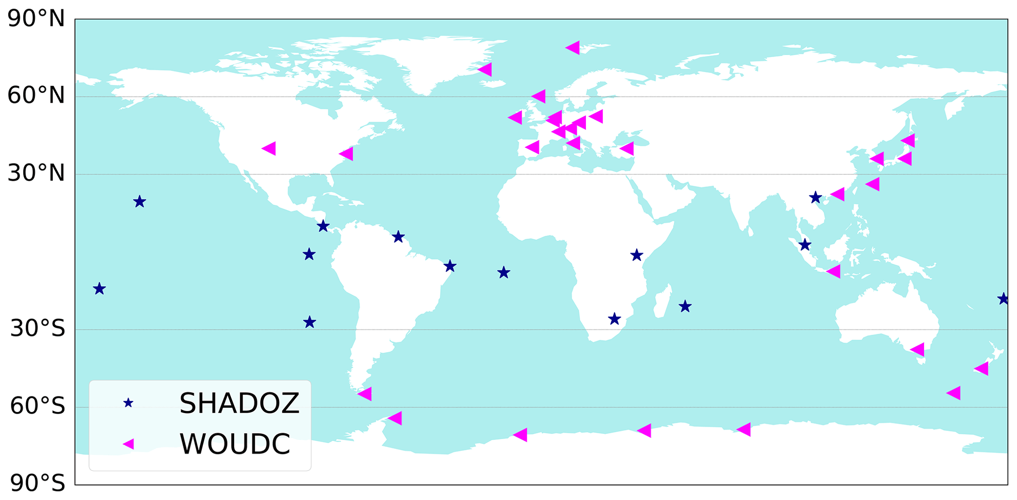
Figure 1Map of the ozonesonde launch sites included in the ozone profile database. Blue stars are the stations from SHADOZ (14 in total) and pink triangles the stations from WOUDC (29 stations). The horizontal lines mark the zonal bands used in the classification of the new ozone climatology.
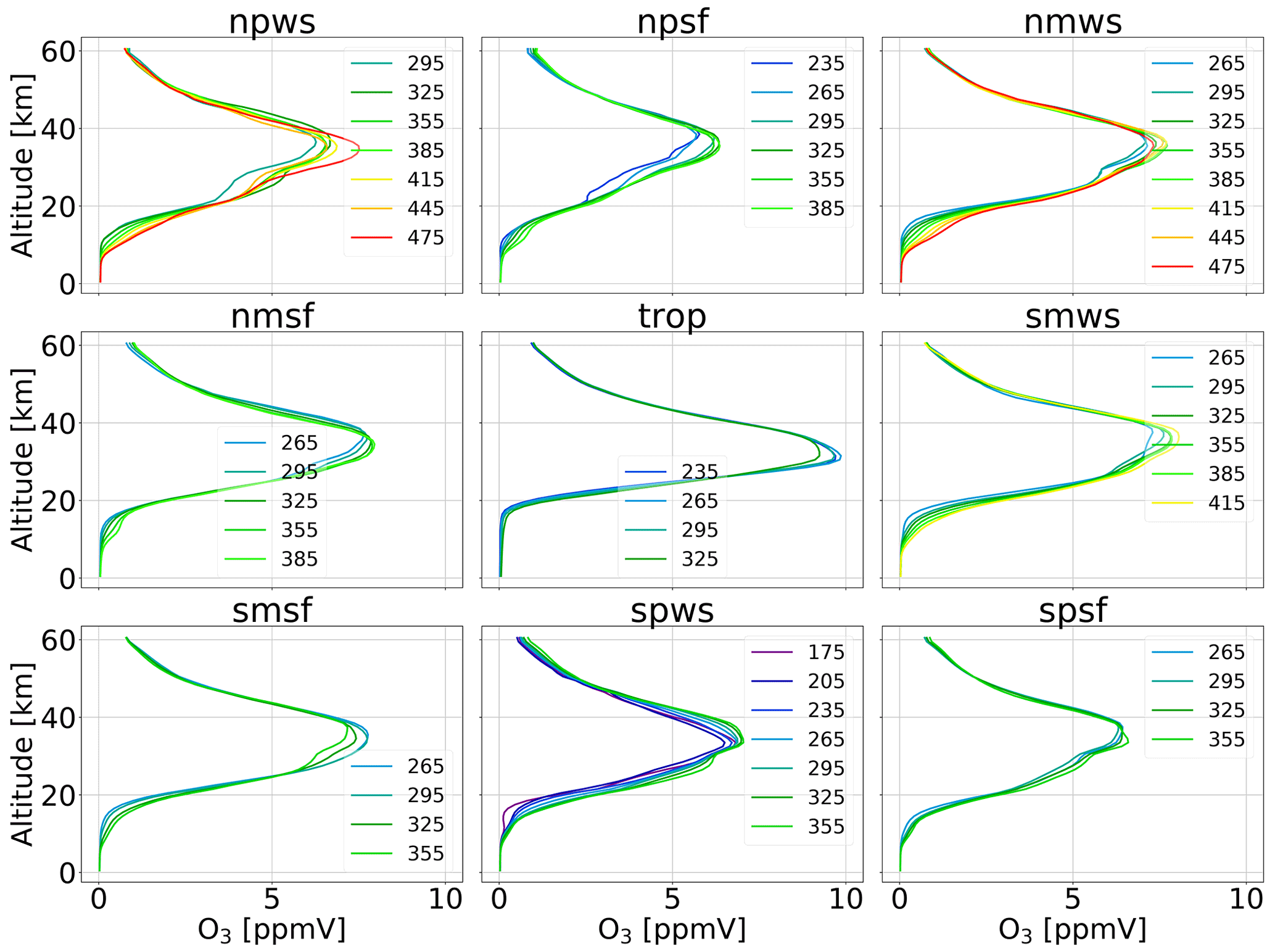
Figure 2Profiles from the ozone a priori database for each latitudinal region, season, and total ozone classification. The labels indicate the total ozone concentration in DU. The titles indicate the region and season (see main text for details).
Every ozone profile in the database was created using the ozonesonde profile up to 11.5 km and the zonal monthly mean limb profile above 20.5 km. In the transition zone between 12.5 and 20.5 km, the merged profile results from a linearly weighted average between the ozonesonde and the limb profile. Each ozonesonde profile was joined with the corresponding zonal monthly mean stratospheric profile, matching the latitude and the month of the ozonesonde. These merged profiles were averaged considering their total ozone content, date, and latitude according to the description above. The resulting ozone climatology profiles in volume mixing ratio units are shown in Fig. 2.
The retrieval algorithm used here is a modification of the weighting function differential optical absorption spectroscopy algorithm (WFDOAS), which has been developed for the retrieval of trace gases in the near-infrared spectrum range from SCIAMACHY measurements (Buchwitz et al., 2000). It was adapted and successfully applied for TOC retrieval in the UV spectral range from nadir-viewing measurements of GOME (Coldewey-Egbers et al., 2005), GOME-2, and SCIAMACHY (Weber et al., 2005; Bracher et al., 2005; Weber et al., 2007).
The algorithm approximates the measured atmospheric optical depth by a Taylor expansion around a first-guess atmospheric state. Also, contributions from interfering species not included in the forward model and a polynomial are included in the fit (Coldewey-Egbers et al., 2005).
For each ground pixel, the natural logarithm of the sun-normalized measured radiance () is fitted by the natural logarithm of the modeled reference intensity (), the weighting functions of ozone () and temperature (), the NO2 cross section as in the standard DOAS approach, the ring spectrum σi,ring, and a low-order polynomial (C). In Eq. (1) the index i references the wavelengths, Vt is the true vertical ozone column, and bt represents the true atmospheric conditions (pressure, temperature, albedo, etc.). is the reference (i.e., used in the forward model) ozone column, is the reference temperature profile, and is the atmospheric state as used in the forward model. ΔV and ΔT represent the corrections to the reference values as a result from the fit. The scalar correction to the temperature profile (ΔT) is a shift applied to the entire vertical temperature profile.
When applying the standard WFDOAS approach to OMPS-NM measurements, the coarse spectral resolution of the latter was found to result in unstable retrievals. To adapt the retrieval technique, it was decided to use a lower-order polynomial, a wider spectral window, and every second spectral point from the input radiance. In the WFDOAS approach, a cubic polynomial is usually used to account for all broadband contributions; consequently, the total column ozone information is obtained from the differential absorption structure only. For OMPS, this resulted in strong variations in the total ozone retrieved from different ground pixels in the across-track direction (for details see Appendix A1). Therefore, a zero-degree polynomial (a constant, C) is used instead of the cubic one, and the broadband spectral signature of ozone absorption is also fitted. To further reduce the impact of the differential ozone absorption structure in the fit, the spectral window was chosen to be 316–336 nm, which is wider than typically used in WFDOAS (325 to 335 nm). In addition, only the odd-numbered spectral points are used in the retrieval, counting from the first spectral point of the selected fitting window (see Appendix A2 for details). Even with a wider spectral window, the use of either all spectral points or the even-numbered ones in some cases resulted in significant discrepancies in the retrieved TOC from ground pixel to ground pixel and in a negative bias of around 2 % with respect to the preferred wavelength selection. The retrieval using the odd-numbered spectral points shows less dependence on the temperature in the fit compared to other wavelength samples (Appendix A2). With these changes, we now refer to the retrieval method as the weighting function fitting approach, WFFA. Apart from using a low-order polynomial and the wider spectral fit window, WFFA is similar to WFDOAS (Coldewey-Egbers et al., 2005). Some further modifications have been implemented, as described below.
The fitting procedure follows an iterative scheme. First, the synthetic radiance and all weighting functions needed in Eq. (1) are computed with a radiative transfer model (RTM). To account for a possible wavelength misalignment between the earthshine spectrum and the solar reference spectrum, the wavelength grid of the earthshine spectrum is adjusted through an iterative nonlinear fit of the shift and squeeze parameters. In the second step, the fit parameters in Eq. (1) (, , , SCDring) and the constant (C) are estimated using a linear least-squares minimization. The resulting total ozone is then passed to the RTM to start the next iteration. The iterative process is terminated when the retrieved ozone column differs by less than 1 DU from the result of the previous iteration.
The reference intensities, as well as the weighting functions, are computed with the RTM SCIATRAN V4.2 (Rozanov et al., 2014) using the ozone profile climatology described in Sect. 3 for a given total ozone, zonal band, and season. During the iterative procedure a new ozone profile is selected according to the retrieved total ozone amount. For each ground pixel, the pressure and temperature profiles are obtained from ECMWF ERA5 (Hersbach et al., 2020). For solar zenith angles (SZAs) larger than 40∘ the pseudo-spherical approximation is employed, whereas for smaller SZAs the plane-parallel atmosphere is used, which is faster. The pseudo-spherical approximation solves the radiative transfer equation for a plane-parallel atmosphere; however, the single-scattering source function is calculated considering the spherical shape of the atmosphere. The ground-level viewing geometry is used in the forward model. Compared with the spherical mode (Rozanov et al., 2000), the use of this approach yields almost identical results (de Beek et al., 2004).
The selected initial-guess value of total ozone for the first pixel processed per FOV is 300 DU. The subsequent pixels use the retrieved TOC from the previous one as an initial value. The ozone absorption cross sections from Serdyuchenko et al. (2014) and the NO2 absorption cross sections from Burrows et al. (1998) are used. An aerosol-free atmosphere is assumed in the model. As in WFDOAS, the effective scene albedo is retrieved near 377 nm using the Lambert equivalent reflectivity (LER) approach (Coldewey-Egbers et al., 2005) (see Appendix A3 for estimation of the related uncertainties).
The ring effect is estimated using the difference in the optical depths calculated by the SCIATRAN model with and without Raman scattering (Rozanov and Vountas, 2014). Lookup tables (LUTs) of radiances accounting for the ring effect, i.e., infilling of Fraunhofer lines and molecular absorption bands, were simulated using SCIATRAN V4.2 and implemented in the retrieval scheme. With the pixel's viewing geometry information, total ozone, surface albedo, and altitude, the LUTs are read and interpolated to obtain the corresponding ring spectrum at high spectral resolution. After convolution of the LUT radiances with and without the ring effect with the instrument response function, the logarithm of the ratio of both convolved radiances is used as the ring spectrum in Eq. (1). A second lookup table provides modeled sun-normalized radiances calculated with and without polarization. From these, correction factors are determined to convert the observed (polarized) radiances into scalar radiances. With the LUTs, the time-consuming RTM modeling of the ring and polarization effects during the retrieval can be avoided. As the ring effect and polarization depend on ozone, the inputs from the LUTs are updated in each iteration.
(Malicet et al., 1995)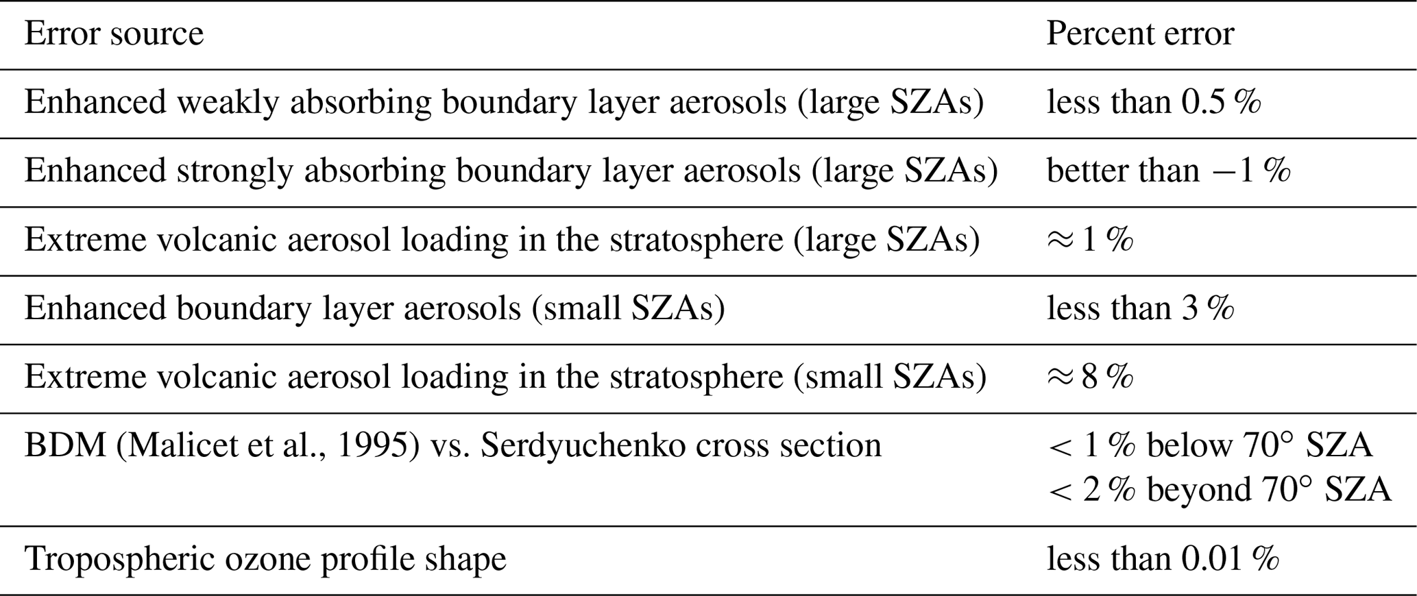
A full analysis of uncertainties and errors was performed for WFDOAS and presented by Coldewey-Egbers et al. (2003). In addition, we checked the major sources of errors that could affect our retrieval differently due to the change in the fitting window. Table 1 presents the results of the sensitivity tests that include enhanced aerosol loading, choice of ozone absorption cross section, and tropospheric ozone profile shape. Details on the enhanced aerosol loading and the tropospheric ozone tests can be found in Appendixes A3 and A4, respectively.
In order to evaluate our scientific product, a comparison with other total ozone column measurements was performed. The NASA product from OMPS-NM, the operational OFFL and scientific WFDOAS products from the Tropospheric Monitoring Instrument on board Copernicus Sentinel-5 Precursor (S5P/TROPOMI), and ground-based Brewer and Dobson measurements were used.
5.1 Ground-based measurements
The comparison with ground-based data was performed using daily means of total ozone columns from 18 Dobson (Basher, 1982) and 30 Brewer (Kerr, 2002) stations, obtained from the WOUDC dataset. Only ozone data derived from direct sun (DS) measurements are included in the analysis as they are the most accurate (Vanicek et al., 2003).
5.2 Operational OMPS-NM total ozone column
The operational OMPS-NM Level 2 (L2) version 2.1 total ozone column product (Jaross, 2017b) is generated using NASA's V8.5 total column retrieval algorithm. This algorithm uses a pair of wavelengths to retrieve cloud fraction and ozone of 317.5 and 331.2 nm for most conditions as well as 331.2 and 360 nm for high amounts of ozone and large SZAs (https://ozoneaq.gsfc.nasa.gov/docs/NMTO3-L2_Product_Description.pdf, last access: 18 August 2021; OMPS Nadir Mapper Level 2 Description). The weak ozone absorption wavelength (331.2 nm) is used to estimate effective surface reflectivity and effective cloud fraction through the mixed Lambert equivalent reflectivity model. The strongly absorbing wavelength (317.5 nm) is used to estimate ozone. The measured radiances are compared with a pre-calculated set of radiances using various ozone and temperature profiles, and the TOC is obtained using piecewise linear interpolation (Bhartia, 2002).
The validation of the NASA data product was presented in McPeters et al. (2019). They performed comparisons with ground-based measurements, Dobson and Brewer stations, and the merged ozone data (MOD) time series (Frith et al., 2014), which, for the period of comparison with OMPS-NM, is a combination of SBUV/2 instruments on three different satellites: NOAA 16, 18, and 19. The comparison with ground-based instruments located in the Northern Hemisphere showed very good agreement with differences to within 0.5 % and an average bias of less than 0.2 % from April 2012 to the end of 2016. Concerning MOD, monthly mean global average showed a bias of −0.2 %.
5.3 S5P/TROPOMI total ozone column
The Sentinel-5 Precursor (S5P) is the first of the atmospheric composition Sentinel satellites as part of the Copernicus Program. It was launched in October 2017 in a sun-synchronous orbit with 13:30 LT ascending node approximately 5 min behind Suomi NPP carrying OMPS. The TROPOspheric Monitoring Instrument (TROPOMI) aboard S5P is a nadir-viewing spectrometer that provides measurements in the ultraviolet, visible, near-infrared, and shortwave infrared spectral bands. TROPOMI has a ground pixel resolution of 3.5 km × 7 km (3.5 km × 5.5 km since August 2019), covering 2600 km across-track (Veefkind et al., 2012).
The L2 product of S5P/TROPOMI used in this study is the offline (OFFL and RPRO) total ozone column product (Lerot et al., 2021). S5P/TROPOMI OFFL and RPRO total ozone are very similar and are obtained using the GODFIT version 4 retrieval (Lerot et al., 2014). The algorithm performs a direct comparison with simulated radiances through nonlinear least-squares inversion using the sun-normalized measured radiance from 325 to 335 nm. The modeled radiances and Jacobians are obtained with the RTM LIDORT (Spurr et al., 2018).
A validation for S5P/TROPOMI OFFL TOC with global ground-based measurements during the period from April to November 2018 showed a mean bias of 0 % to 1.5 % and standard deviations between 2.5 % and 4.5 % for monthly mean co-locations (Garane et al., 2019).
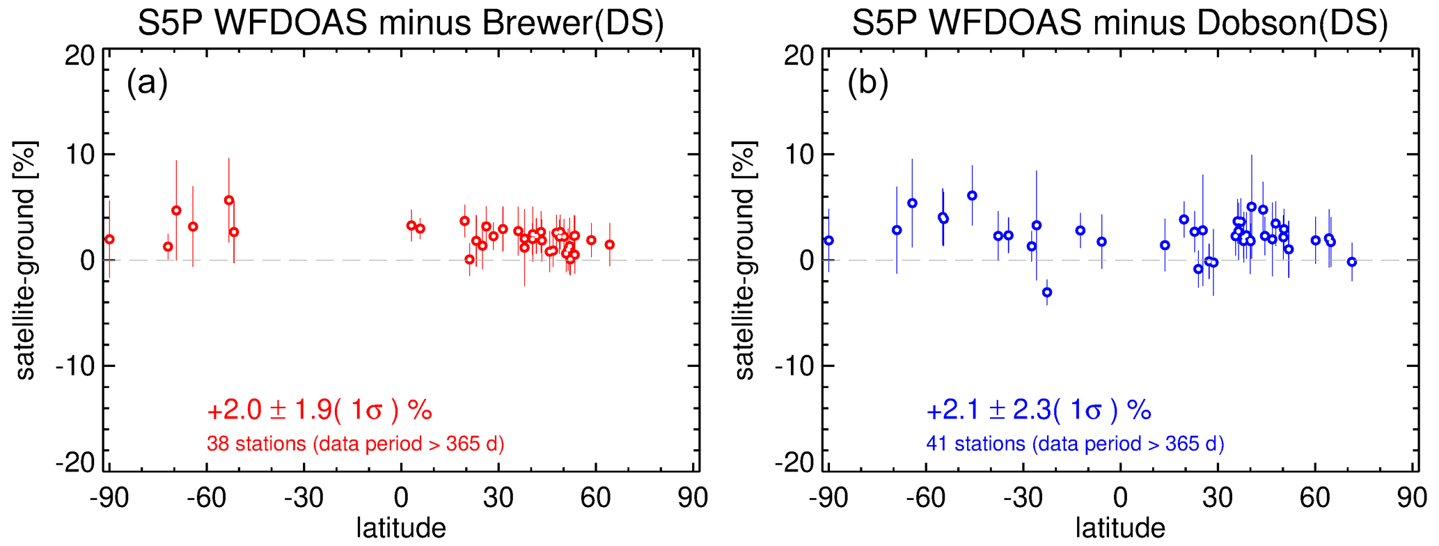
Figure 3Summary of the daily mean comparison between ground-based measurements and S5P/TROPOMI WFDOAS TOC for Brewer (a) and Dobson (b) instruments.
A scientific S5P/TROPOMI product generated with the WFDOAS v4 algorithm was also used. The WFDOAS setup is identical to WFFA described above except for the narrower wavelength window (325–335 nm) and a third-degree polynomial used (Eq. 1). Furthermore, WFDOAS uses temperature profiles reported with the ozone profile climatology rather than reanalysis data as in WFFA. Figure 3 shows a comparison of S5P/TROPOMI WFDOAS results with daily ground-based measurements between November 2017 and September 2019. S5P/TROPOMI-WFDOAS shows a bias of 2.0 % with 1σ of 1.9 % for Brewer instruments and 2.1 % bias with 2.3 % standard deviation for Dobson instruments.
To perform the comparison with ground-based data and between the S5P products, both datasets, OFFL and WFDOAS, have been binned into 0.3∘ × 0.3∘ boxes and averaged daily. These gridded data were also used for the comparison with OMPS-WFFA retrieval. Figure 4 shows the latitude–time comparison between TROPOMI WFDOAS and OFFL, exhibiting a global mean difference of 1.5 % with 0.7 % standard deviation, with WFDOAS being higher than OFFL. Almost no seasonal variability is observed in the differences, and larger differences occur in the Southern Hemisphere polar region during winter–spring.
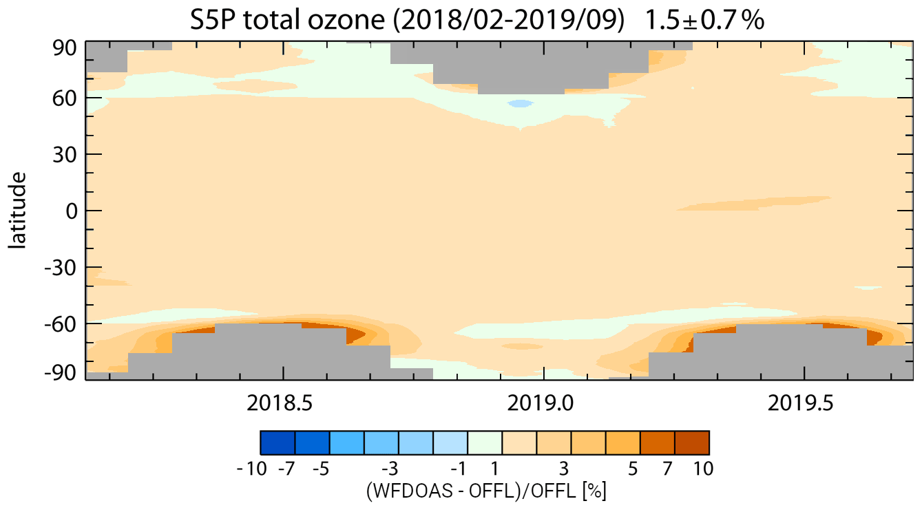
Figure 4Latitude–time comparison between S5P/TROPOMI OFFL and S5P/TROPOMI WFDOAS total ozone from February 2018 to September 2019.
The S5P-WFDOAS product is retrieved using the Serdyuchenko et al. (2014) ozone absorption cross sections. For the WFDOAS approach, the use of the Bass–Paur (BP, shifted by 0.23nm) and BDM (Brion–Daumont–Malicet) ozone absorption cross sections (Paur and Bass, 1985; Malicet et al., 1995) leads to retrieved total ozone being lower by 2 %–3 %. We note that the WFFA approach with a wider spectral window and subtraction of a low-order polynomial is weakly sensitive to the use of different ozone absorption cross sections.
A total of 3 years (2016–2018) of OMPS/WFFA TOC data were daily averaged and gridded onto a 0.5∘ × 0.5∘ grid to perform the analysis and compare with other products. For the validation, percentage differences with respect to comparison datasets were calculated as follows: .
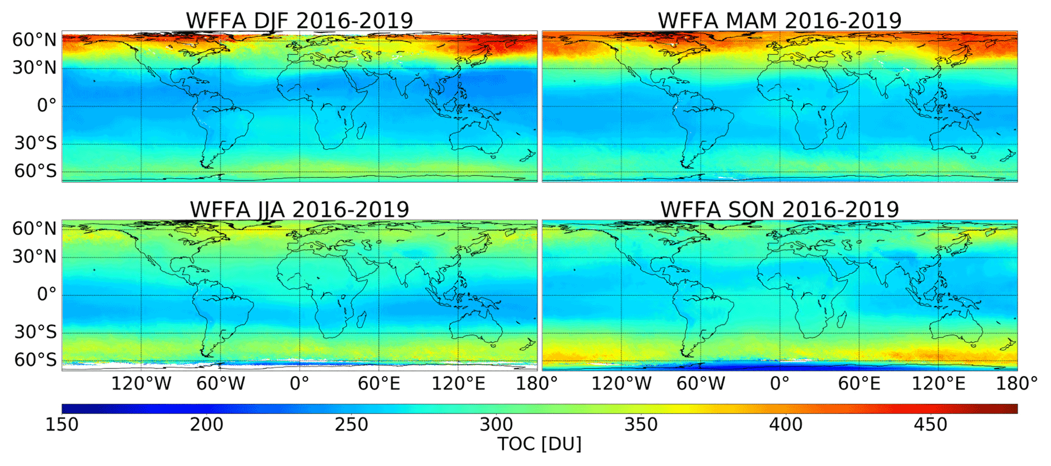
Figure 5Seasonal average maps of WFFA/OMPS-NM total ozone column.
Figure 5 shows seasonal maps of WFFA TOC for the analyzed period. The total ozone generally shows a minimum in the tropical region in all seasons. The meridional gradient of TOC is stronger during winter and spring for both hemispheres. In the subpolar region of the Northern Hemisphere, increased ozone values are observed during DJF and MAM. In the Southern Hemisphere, over the subpolar region, the maximum in TOC during austral spring (SON) is weaker than its counterpart in the Northern Hemisphere. The minimum over the Antarctic during austral spring (“ozone hole”) is observed. Over complex topography areas, like the Himalayas in Asia and the Andes in South America, lower ozone amounts are observed.
6.1 Comparison with ground-based measurements
Daily mean ground-based data for 48 stations were compared with daily satellite data averaged in the grid box that contains the station. Since only cloud-free satellite ground pixels were retrieved, the number of co-located days to be compared at a given station is rather low. Only stations with co-located data for at least 70 d were selected to have a sufficient sample for the comparison. With these criteria, 18 Dobson and 30 Brewer stations were available for the validation during the analyzed period.
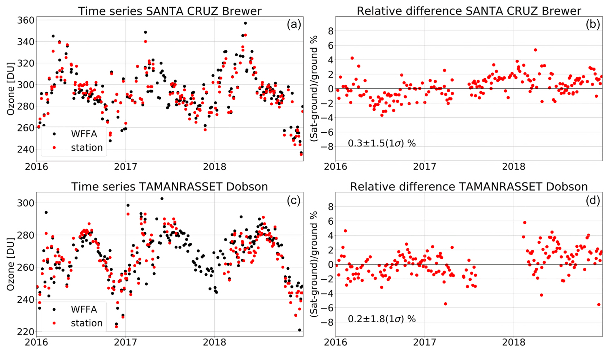
Figure 6(a, c) Examples of daily mean total ozone time series from ground-based measurements (red) and co-located WFFA TOC (black) from 2016 to 2018 in Santa Cruz (28.42∘ N, 16.26∘ W) and Tamanrasset (22.80∘ N, 5.52∘ E). (b, d) Percentage differences between WFFA and ground-based data. Mean relative difference and its standard deviation are indicated.
Daily relative differences between WFFA TOC and the ground-based data were calculated. The mean relative differences vary from −2 % for Rio Gallegos (Brewer; 51.60∘ S, 69.32∘ W) to 4.8 % for Mauna Loa (Brewer; 19.53∘ N, 155.57∘ W). The high bias with respect to Mauna Loa data might result from the station's high altitude (3.4 km), while the grid box's average surface height is much lower (1.0 km). The standard deviation varies from 0.8 % for Paramaribo (Brewer; 5.81∘ N, 55.21∘ W) to 6.6 % for Amberd (Dobson; 40.38∘ N, 44.25∘ E). Figure 6 shows the time series and the relative differences for two selected stations as an example of the comparison: Santa Cruz (Brewer; 28.42∘ N, 16.26∘ W) and Tamanrasset (Dobson; 22.80∘ N, 5.52∘ E). Figure 6 shows that the seasonality of both WFFA and ground-based data is similar. Very good agreement in the seasonality and the TOC values is observed for all considered ground stations. From a total of 48 stations, 28 show a bias of less than 1 %, and 27 stations show standard deviations of less than 3 %.
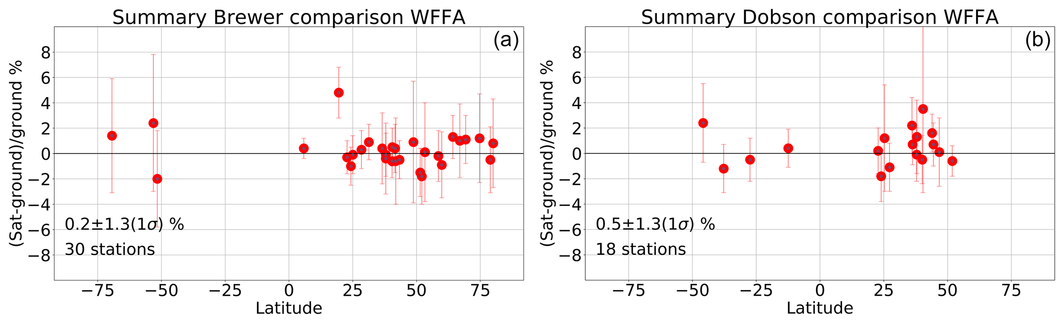
Figure 7Summary of the mean relative differences between WFFA results and ground-based measurements for Brewer (a) and Dobson (b) instruments from 2016 to 2018. Mean differences and their standard deviations are indicated along with the number of stations analyzed.
Figure 7 presents the summary of the comparisons with Brewer (left) and Dobson instruments (right) as a function of latitude. A distinction between the instruments was made because they might show differences of up to 4 % in their direct sun measurements (Feister, 1994; Vanicek, 2006). Overall, the bias between WFFA and ground-based measurements is positive at 0.2 % for Brewer and 0.5 % for Dobson instruments, with a mean standard deviation of 1.3 %. For stations with both instruments, which are Athens (37.98∘ N, 23.73∘ E) and Tamanrasset (22.80∘ N, 5.52∘ E), the differences between Dobson and Brewer are 1.7 % and 0.5 %, respectively. No particular patterns between hemispheres are observed. Averaging all stations, WFFA TOC exhibits a mean bias of 0.3 ± 1.3 (1σ) %.
6.2 Comparison with OMPS-NM operational product and S5P/TROPOMI
WFFA results have been compared to the operational total ozone column product of OMPS-NM L2 v2.1 (OMPS-L2) and two different retrievals from S5P/TROPOMI (OFFL and WFDOAS) as introduced in Sect. 5.
A comparison for one orbit on 10 June 2018 is shown in Fig. 8. The upper panels show the TOC of the central across-track FOV (18) against latitude and SZA for all datasets. The lower panels show the percentage differences of WFFA results with respect to the comparison datasets. The ozone total column reaches a minimum in the tropics increasing towards the poles, with local maxima at 40∘ S and 70∘ N. The absolute maximum is observed at 50∘ N. All satellite data show very good agreement in the variation of TOC with latitude and SZA. The mean bias with respect to OMPS-L2 is 0.39 %. The differences with respect to S5P OFFL and WFDOAS data are −0.36 % and −2.48 %, respectively. S5P WFDOAS exhibits more ozone than the other datasets along the entire orbit. This is expected considering the direct comparisons between the two S5P datasets shown above (Sect. 5.3). Between −70 and 40∘ SZAs (approximately 40∘ S to 60∘ N in latitude), differences with respect to OMPS L2 and S5P OFFL data vary around ±1 %. For larger SZAs, WFFA results differ by less than 2 % with respect to the three comparison datasets, except for the first pixel of the considered orbit. A difference between hemispheres is observed; for the Northern Hemisphere WFFA shows more ozone than S5P OFFL and OMPS-L2, while for the Southern Hemisphere WFFA TOC is lower. The standard deviations of the differences are similar for all three comparison datasets, varying between 1.1 % for OMPS-L2 and 1.4 % for S5P WFDOAS.

Figure 8Ozone total column (a, b) and percentage differences (c, d) for an example orbit against latitude (a, c) and SZA (b, d) for the central FOV (18) of the orbit. OMPS orbit number 34298 on 10 June 2018. Southern Hemisphere SZA values are plotted as negative numbers for clarity.
To carry out a more general comparison by looking at seasonal and global averages, the three comparison datasets were gridded in the same way as WFFA data. For OMPS-L2 the same orbits and ground pixels as those for WFFA were selected (ground pixels with cloud fraction less than 0.1, SZA smaller than 80∘, and only across-track FOVs from 10 to 22) from 2016 to 2018. For S5P all available data (all FOVs and cloudy scenes included) were gridded. The regular production of the OFFL data started on 30 April 2018. To compare an entire 12-month period, WFFA TOC was retrieved until May 2019. Thus, the comparison with S5P/TROPOMI OFFL and WFDOAS comprised data from June 2018 until May 2019. The comparison was only made for daily grid boxes with data available for WFFA.
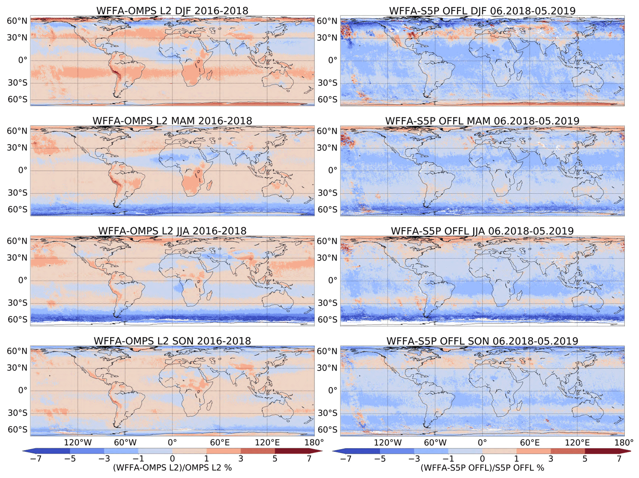
Figure 9Relative differences in the total ozone column between the seasonally averaged WFFA data and two other satellite products. Left panel: relative differences with respect to OMPS-L2. Right panel: relative differences with respect to S5P OFFL.
Figure 9 shows maps of seasonal relative deviations of WFFA results compared to those from OMPS-L2 (left) and S5P OFFL (right). In general, WFFA has a positive bias with respect to OMPS L2 and a negative with respect to S5P OFFL. Larger differences are observed in the polar regions. During austral autumn and winter (MMA and JJA) WFFA TOC is lower than the other two satellite datasets in the polar region, while during the austral summer (DJF) is higher. Over areas with complex topography, like the Himalayas in Asia, the Great Rift Valley in Africa, and the Andes in South America, WFFA ozone values are larger than OMPS-L2 by up to 6 % but are in good agreement with S5P OFFL. As it was seen in Fig. 5, WFFA shows lower ozone for scenes with high surface elevation than in the surrounding areas, the same was observed for OMPS-L2 (not shown) with even lower values than WFFA, which explain the larger differences over, for example, the Andes.
From the differences of WFFA with respect to OMPS-L2, a positive bias over both poles and a bias of around 4 % in southern subtropics and at northern midlatitudes are observed during boreal winter. Globally a mean positive bias of 0.6 ± 1.5 (1σ) % is observed. During boreal spring, the bias dissipates in the southern subtropics and becomes less persistent at northern midlatitudes. Combined with larger negative differences in the southern polar area, this results in a global mean bias of 0.2 ± 1.3 (1σ) % for MAM. In boreal summer, a 2 % bias is observed in the northern subtropics, decreasing in autumn (SON). The higher bias in the summer hemisphere's subtropical areas is possibly related to the Intertropical Convergence Zone (ITCZ). Although only cloud-free scenes are retrieved, some of the ground pixels may still be contaminated by clouds, which might result in small systematic biases. The yearly global mean difference is 0.0 ± 1.3 %.
The comparison between WFFA and S5P/TROPOMI results is shown in the right panels of Fig. 9. Striping is seen in the differences to S5P, most likely due to differences in the grid boxes' sampling. For S5P, the topography distinction is seen over the Andes and the Himalayas only during boreal winter and spring. Patterns similar to those observed for OMPS L2 are seen over the polar regions, except in the northern pole during boreal winter when S5P OFFL TOC is up to 4 % higher than WFFA. The subtropical positive bias band observed for OMPS-L2 is negative and within 1 % for S5P OFFL. For areas where WFFA TOC is less than OMPS-L2 TOC, like over southern subtropics during austral winter, S5P OFFL shows even higher values. The global mean relative differences with respect to S5P OFFL are −0.6 ± 1.5 (1σ) for DJF, −0.8 ± 1.5 (1σ) for MAM, −0.8 ± 1.2 (1σ) for JJA, and −0.8 ± 1.5 (1σ) for SON.
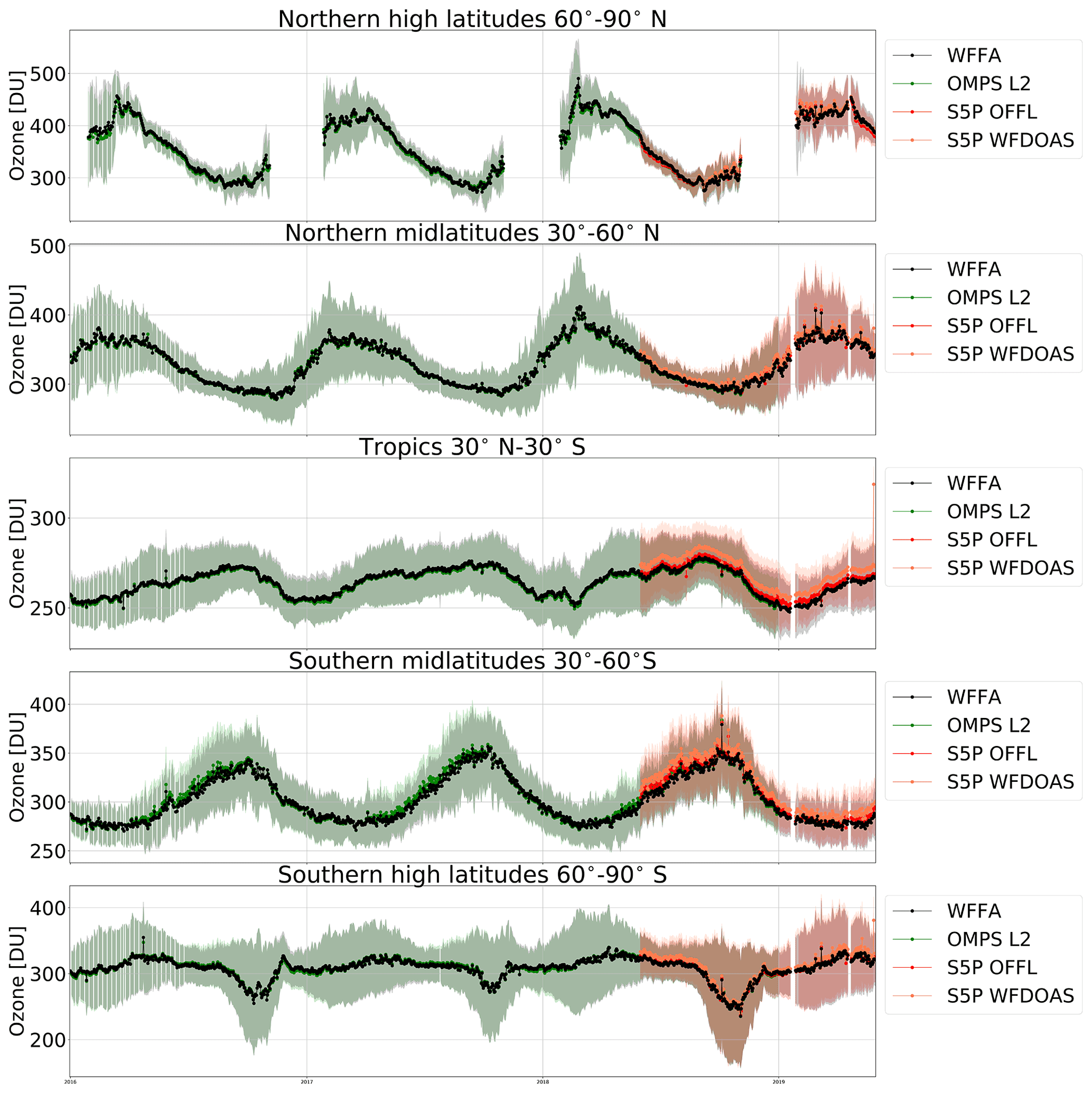
Figure 10Zonal mean time series of WFFA, OMPS-L2, S5P OFFL, and S5P WFDOAS TOC for five latitudinal bands. The shading indicates the standard deviations of the time series.

Figure 11Differences of the zonal mean time series of WFFA with respect to the results from OMPS-L2, S5P OFFL, and S5P WFDOAS for five latitudinal bands. The shading indicates the standard deviations of the time series.
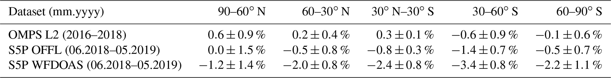
Table 2Relative differences and standard deviations between WFFA/OMPS-NM and OMPS L2, S5P/TROPOMI OFFL, and S5P/TROPOMI WFDOAS in various zonal bands.
For a more detailed analysis, TOC time series for five zonal bands were calculated: high northern latitudes (60–90∘ N), northern midlatitudes (30–60∘ N), tropics (30∘ N–30∘ S), southern midlatitudes (30–60∘ S), and southern high latitudes (60–90∘ S), as shown in Fig. 10. The mean relative differences in these zonal bands are shown in Fig. 11 and summarized in Table 2. In general, the four different datasets follow the same seasonality and short-term variability, generally showing very good agreement. However, the S5P products OFFL and WFDOAS are typically higher than OMPS-L2 and WFFA, particularly in the tropics and at southern midlatitudes. A persistent mean negative bias is observed with respect to S5P WFDOAS, as seen in the comparison for one sample orbit in Fig. 8.
Figure 11 shows larger variations at high northern latitudes, particularly during boreal winter. Nevertheless, the mean differences in the 60–90∘ N band are 0 % with respect to S5P-OFFL and less than 1.2 % for the other datasets. At northern midlatitudes, WFFA shows a bias of 0.2 % with respect to OMPS-L2, −0.5 % with respect to S5P-OFFL, and −2.0 % with respect to S5P-WFDOAS. In the tropics, the differences between the datasets are fairly constant with time, with biases of 0.3 % for OMPS-L2, −0.8 % for S5P-OFFL, and −2.4 % for S5P-WFDOAS; the standard deviations are below 0.8 %. At southern midlatitudes, WFFA shows less ozone than OMPS-L2 during winter by about −3 %. The relative difference decreases in autumn and spring and becomes slightly positive during the summer. The same pattern is observed when comparing with S5P, with the mean relative differences ranging from −1.4 for OFFL to −3.4 % for WFDOAS. At high southern latitudes, WFFA results show similar seasonal behavior as in the midlatitudes. Overall there is a −0.1 % bias with respect to OMPS-L2, and the standard deviation is 0.6 % (1σ). Very good agreement (bias −0.5 %) of both WFFA and OMPS-L2 with S5P-OFFL is observed at these latitudes.
In this study we present a new scientific TOC product from OMPS-NM observations using the WFFA technique, which is a modified retrieval approach adapted from the WFDOAS algorithm. A new ozone profile climatology was generated for the retrieval using OMPS-LP profiles (Arosio et al., 2018) and ozonesondes.
OMPS-WFFA data were validated using ground-based measurements from the WOUDC dataset and three other TOC satellite datasets: OMPS-NM Level 2, S5P/TROPOMI OFFL, and S5P/TROPOMI WFDOAS. The comparison with ground-based measurements shows a mean bias below 1 % for 28 of a total of 48 stations. For 27 stations, the standard deviations of the mean differences are under 3 %. In total, a mean bias of +0.3 % and a standard deviation of 1.3 % were found. These values are similar to those reported by the operational product of OMPS-NM and by S5P/TROPOMI (Sect. 5). All comparisons between WFFA TOC and other satellite products are consistent concerning seasonality and variability with latitude. WFFA TOC presents a zero yearly global mean bias with respect to OMPS-L2, approximately −0.6 % with respect to S5P OFFL, and −2.5 % with respect to S5P WFDOAS. The standard deviations of the differences are around 1.4 % for all satellite validation datasets. Larger differences were found for polar regions and larger SZAs.
The newly created WFFA OMPS-NM total ozone dataset is intended to be used for retrieving tropospheric ozone columns employing the limb–nadir matching technique in combination with OMPS-LP data.
A1 From WFDOAS to WFFA
The use of the original WFDOAS approach in the typical spectral window (325 to 335 nm) with OMPS-NM data results in large variations of the retrieved TOC for different across-track ground pixels. Figure A1 shows ozone anomalies (TOC value minus the mean of all across-track FOVs) for all the orbits of 1 d, averaged over the tropics (10∘ S–10∘ N) as a function of the across-track index. The left panel shows the results from the original WFDOAS approach using a cubic polynomial and the spectral window 325 to 335 nm. There are systematic differences between ground pixels: for instance, more than 5 DU differences between FOVs 18 and 19. The results using a cubic polynomial and wider window (316 to 336 nm) are shown in the central panel. For this configuration, the differences between adjacent pixels are smaller, but a large variation of about 30 DU is observed from the first to the last across-track FOV. The right panel shows the results from the WFFA approach using a constant instead of the cubic polynomial and the fitting window from 316 to 336 nm. The variation between pixels is below 2 DU for across-track FOVs 10 to 22.
A2 All, even, and odd spectral points
Table A1 shows the wavelengths used in the fit for the central across-track FOV (18) for the cases of all, even, and odd spectral points. Since the nonlinear fit adjusts the earthshine spectrum's wavelength grid to the solar reference spectrum, the final wavelength grid is different for every across-track FOV.
The selection of the odd-numbered spectral points was made after investigating the effect of the various wavelength choices on the retrieval. When using odd-numbered wavelengths, the retrieval result does not change much whether the temperature fit parameter is included in the fit or not. For the same orbits as used in the previous section (Sect. A1), the retrieval was applied with and without fitting the temperature parameter for the three wavelength selections. Figure A2 shows the relative differences of the results with and without the temperature parameter. The left panel shows the average difference over the across-track FOVs used in this study as a function of latitude. The average over the tropics as a function of the across-track index is shown in the right panel. It is observed that the dependence on the temperature of the odd sample is significantly weaker both across- and along-track. Below 40∘ N and for the central FOVs, the differences for the odd sample are less than 0.5 %, while for the other two datasets, they are between 0.5 % and 1 %. In the standard WFFA retrieval using the odd-numbered wavelength sample, as shown in the main part of the paper, the temperature is still included in the fit procedure.
A3 Sensitivity to aerosol scenarios
The Lambertian equivalent reflectivity (LER) effective scene albedo represents a first-order correction for non-absorbing aerosols. For the WFDOAS technique, the ozone might be underestimated by 1 % in the presence of absorbing aerosols with a visibility of 2 km (Coldewey-Egbers et al., 2003). Since the WFFA approach is slightly different from WFDOAS, similar sensitivity tests using different aerosol scenarios were performed to confirm the prior results.
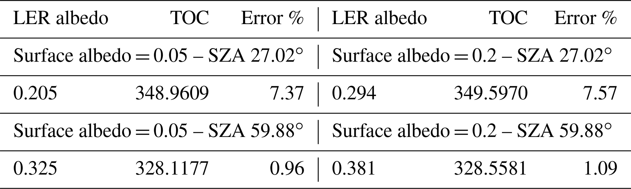
We generated synthetic radiances for different aerosol scenarios using SCIATRAN V4.2 with the aerosol parameterization from LOWTRAN (Kneizys et al., 1988; Shettle and Fenn, 1979). From these radiances, the LER albedo was retrieved and used in the WFFA retrieval. The synthetic radiances were calculated with a total ozone of 325 DU, solar zenith angles of 59.88 and 27.02∘ (chosen from real values of OMPS-NM ground pixels), visibility of 2 km, and surface albedos of 0.05 and 0.2. The different types of boundary layer aerosols are maritime, rural, tropospheric, and urban. One case with extreme volcanic stratospheric aerosol loading was included. The results are summarized in Table A2 for the boundary layer scenarios and in Table A3 for the stratospheric loading.
For large SZAs, the aerosol effect is largely accounted for with the effective scene albedo, particularly for weakly absorbing boundary layer aerosols (urban). In the case of strongly absorbing boundary layer aerosols, uncertainties are somewhat larger but still within 1 %. For small SZAs, the retrieved TOC might be overestimated by about 3 % for weakly absorbing aerosols and by 1 % for strongly absorbing aerosols. In the case of an extreme volcanic aerosol loading in the stratosphere, the retrieved TOC might be overestimated by about 8 % for small SZAs and by about 1 % for large SZAs.
A4 Sensitivity to tropospheric ozone
To investigate the sensitivity of the retrieval to the tropospheric ozone amount, we scaled the lower part of the climatological ozone profiles (below 12 km) by factors of 2 and 5 and repeated the retrieval. At each iterative step the ozone profile to be used in the forward model is extracted from the climatology in accordance with the total ozone column value obtained at the previous iteration (300 DU for the first iteration), and its lower part is scaled as described above. No significant differences in the retrieved total ozone value were identified.
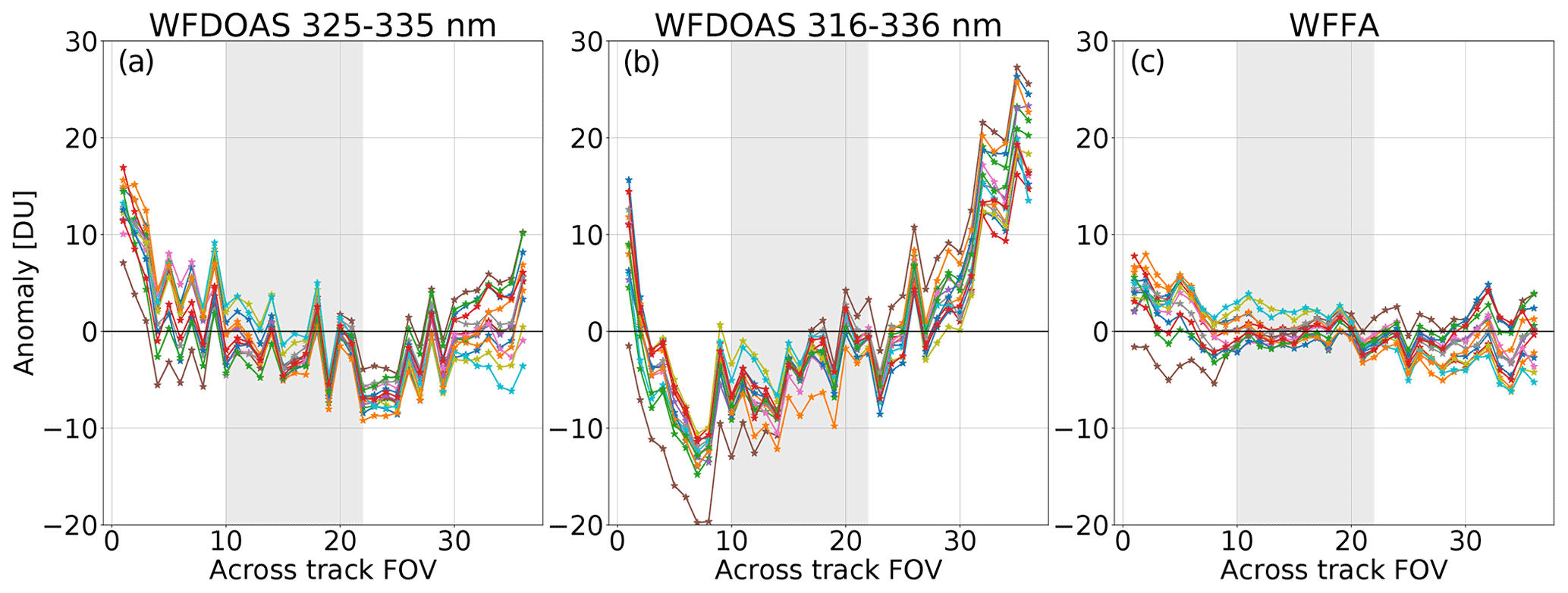
Figure A1Tropical averaged ozone anomalies for all orbits of 1 d (10 January 2018) for different configurations of the retrieval. The grey shading indicates the FOVs used in this study. (a) Original WFDOAS. (b) WFDOAS with a wider spectral window. (c) WFFA.
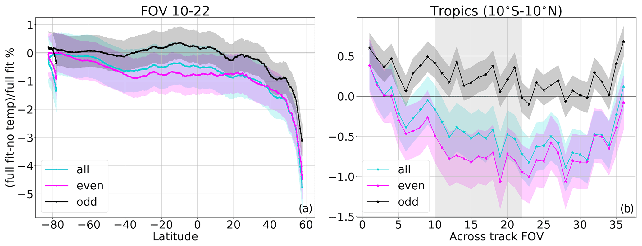
Figure A2Mean relative differences between the results from the fits including and excluding the temperature for the orbits of 1 d (10 January 2018) for different wavelength samples used. (a) Average over the across-track FOVs 10 to 22 as a function of latitude. (b) Average over the tropics as a function of the across-track index. Standard deviations are shown by shadings.
Table A1Wavelengths processed in the retrieval for the FOV 18 in the cases of all, even-, or odd-numbered spectral points (nm).
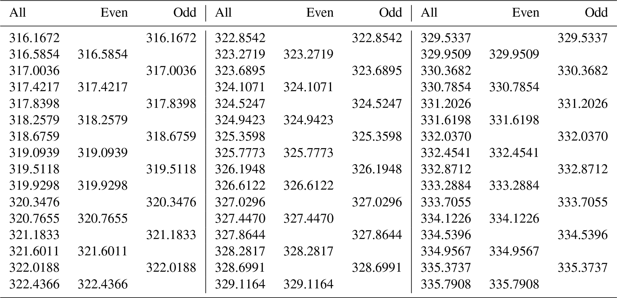
Table A2Results and errors for different boundary layer aerosol scenarios. The true value of TOC is 325 DU.
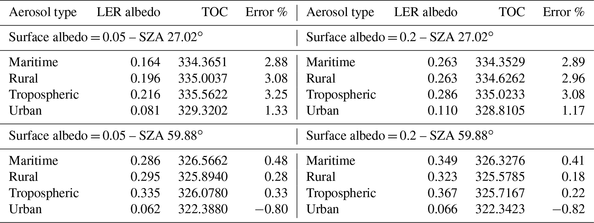
Table A3Results and errors for extreme volcanic stratospheric aerosol loading. The true value of TOC is 325 DU.
The ozone and temperature climatology is available at http://www.iup.uni-bremen.de/UVSAT/datasets/iup-ozone-profile-climatology (Orfanoz-Cheuquelaf et al., 2021).
All authors contributed to the design of the study. AOC developed the retrieval algorithm, performed the computer calculations, and made the comparisons supervised by MW, AR, and ALW with JPB providing scientific conceptual input and oversight. CA provided vertical ozone profiles used in the study from inversions of OMPS-LP observations. AOC led the preparation of the paper. All authors contributed to the writing, editing, and evolution of the paper.
The authors declare that they have no conflict of interest.
Publisher's note: Copernicus Publications remains neutral with regard to jurisdictional claims in published maps and institutional affiliations.
Carlo Arosio acknowledges support from the PRIME program of the German Academic Exchange Service (DAAD) via funds from the German Federal Ministry of Education and Research (BMBF) and ESA's Living Planet Fellowship SOLVE. Most of the calculations reported here were performed on HPC facilities of the IUP, University of Bremen. The limb ozone profiles were processed on the German HLRN (High-Performance Computer Center North). The GALAHAD Fortran library was employed in the retrieval scheme.
This research has been supported by the University and the State of Bremen, ESA-Ozone-CCI+, BMBF SynopSys-Ozone, and the German Research Foundation (DFG; research unit VolImpact (FOR2820), project VolARC, grant nos. INST 144/379-1 and INST 144/493-1).
The article processing charges for this open-access publication were covered by the University of Bremen.
This paper was edited by Michel Van Roozendael and reviewed by three anonymous referees.
Arosio, C., Rozanov, A., Malinina, E., Eichmann, K.-U., von Clarmann, T., and Burrows, J. P.: Retrieval of ozone profiles from OMPS limb scattering observations, Atmos. Meas. Tech., 11, 2135–2149, https://doi.org/10.5194/amt-11-2135-2018, 2018. a, b, c, d, e
Basher, R. E.: WMO Global Ozone Reseaech and Monitoring Project. Report No. 13. Review of the Dobson Spectrophotometer and its Accuracy, Tech. rep., World Meteorological Organization WMO, Geneva, available at: https://www.esrl.noaa.gov/gmd/ozwv/dobson/papers/report13/report13.html (last access: 4 September 2020), 1982. a
Bhartia, P. K.: OMI Algorithm Theoretical Basis Document, Tech. Rep. ATBD-OMI-02, NASA Goddard Space Flight Center, Greenbelt, Maryland, USA, 2002. a, b
Bovensmann, H., Burrows, J. P., Buchwitz, M., Frerick, J., Noël, S., Rozanov, V. V., Chance, K. V., and Goede, A. P. H.: SCIAMACHY: Mission Objectives and Measurement Modes, J. Atmos. Sci., 56, 127–150, https://doi.org/10.1175/1520-0469(1999)056<0127:SMOAMM>2.0.CO;2, 1999. a
Bracher, A., Lamsal, L. N., Weber, M., Bramstedt, K., Coldewey-Egbers, M., and Burrows, J. P.: Global satellite validation of SCIAMACHY O3 columns with GOME WFDOAS, Atmos. Chem. Phys., 5, 2357–2368, https://doi.org/10.5194/acp-5-2357-2005, 2005. a, b
Bramstedt, K., Gleason, J., Loyola, D., Thomas, W., Bracher, A., Weber, M., and Burrows, J. P.: Comparison of total ozone from the satellite instruments GOME and TOMS with measurements from the Dobson network 1996–2000, Atmos. Chem. Phys., 3, 1409–1419, https://doi.org/10.5194/acp-3-1409-2003, 2003. a
Buchwitz, M., Rozanov, V. V., and Burrows, J. P.: A near-infrared optimized DOAS method for the fast global retrieval of atmospheric CH4, CO, CO2, H2O, and N2O total column amounts from SCIAMACHY Envisat-1 nadir radiances, J. Geophys. Res.-Atmos., 105, 15231–15245, https://doi.org/10.1029/2000JD900191, 2000. a
Burrows, J. P., Hölzle, E., Goede, A. P., Visser, H., and Fricke, W.: SCIAMACHY-scanning imaging absorption spectrometer for atmospheric chartography, Acta Astronaut., 35, 445–451, https://doi.org/10.1016/0094-5765(94)00278-T, 1995. a
Burrows, J. P., Dehn, A., Deters, B., Himmelmann, S., Richter, A., Voigt, S., and Orphal, J.: Atmospheric remote-sensing reference data from GOME: part 1. Temperature-dependent absorption cross-sections of NO2 in the 231–794 nm range, J. Quant. Spectrosc. Ra., 60, 1025–1031, https://doi.org/10.1016/S0022-4073(97)00197-0, 1998. a
Burrows, J. P., Weber, M., Buchwitz, M., Rozanov, V., Ladstätter-Weißenmayer, A., Richter, A., DeBeek, R., Hoogen, R., Bramstedt, K., Eichmann, K.-U., and Eisinger, M.: The Global Ozone Monitoring Experiment (GOME): Mission, instrument concept, and first scientific results, European Space Agency, (Special Publication) ESA SP, 56, 151–175, https://doi.org/10.1175/1520-0469(1999)056<0151:TGOMEG>2.0.CO;2, 1999. a
Coldewey-Egbers, M., Weber, M., Lamsal, L. N., Beek, R. D., Buchwitz, M., and Burrows, J. P.: WF-DOAS Algorithm Theoretical Basis Document, Tech. rep., Institute of Environmental Physics, University of Bremen, Bremen, Germany, https://doi.org/10.26092/elib/381, 2003. a, b
Coldewey-Egbers, M., Weber, M., Lamsal, L. N., de Beek, R., Buchwitz, M., and Burrows, J. P.: Total ozone retrieval from GOME UV spectral data using the weighting function DOAS approach, Atmos. Chem. Phys., 5, 1015–1025, https://doi.org/10.5194/acp-5-1015-2005, 2005. a, b, c, d
de Beek, R., Weber, M., Rozanov, V., Rozanov, A., Richter, A., and Burrows, J.: Trace gas column retrieval – an error study for GOME-2, Adv. Space Res., 34, 727–733, https://doi.org/10.1016/j.asr.2003.06.042, 2004. a
Ebojie, F., von Savigny, C., Ladstätter-Weißenmayer, A., Rozanov, A., Weber, M., Eichmann, K.-U., Bötel, S., Rahpoe, N., Bovensmann, H., and Burrows, J. P.: Tropospheric column amount of ozone retrieved from SCIAMACHY limb–nadir-matching observations, Atmos. Meas. Tech., 7, 2073–2096, https://doi.org/10.5194/amt-7-2073-2014, 2014. a
Feister, U.: Comparison between Brewer spectrometer , M 124 filter ozonometer and Dobson spectrophotometer, in: Ozone in the Troposphere and Stratosphere, April 1994, 770–773, available at: https://ui.adsabs.harvard.edu/abs/1994ozts.nasa..770F (last access: 27 October 2020), 1994. a
Fioletov, V. E., Kerr, J. B., Hare, E. W., Labow, G. J., and McPeters, R. D.: An assessment of the world ground-based total ozone network performance from the comparison with satellite data, J. Geophys. Res.-Atmos., 104, 1737–1747, https://doi.org/10.1029/1998JD100046, 1999. a
Fishman, J. and Larsen, J. C.: Distribution of total ozone and stratospheric ozone in the tropics: Implications for the distribution of tropospheric ozone, J. Geophys. Res., 92, 6627, https://doi.org/10.1029/JD092iD06p06627, 1987. a
Flynn, L., Hornstein, J., and Hilsenrath, E.: The ozone mapping and profiler suite (OMPS), in: IEEE International IEEE International IEEE International Geoscience and Remote Sensing Symposium, 2004. IGARSS '04, 20–24 September 2004, Anchorage, AK, USA, Proceedings, vol. 1, 152–155, IEEE, https://doi.org/10.1109/IGARSS.2004.1368968, 2004. a, b
Flynn, L., Long, C., Wu, X., Evans, R., Beck, C. T., Petropavlovskikh, I., McConville, G., Yu, W., Zhang, Z., Niu, J., Beach, E., Hao, Y., Pan, C., Sen, B., Novicki, M., Zhou, S., and Seftor, C.: Performance of the Ozone Mapping and Profiler Suite (OMPS) products, J. Geophys. Res.-Atmos., 119, 6181–6195, https://doi.org/10.1002/2013JD020467, 2014. a
Frith, S. M., Kramarova, N. A., Stolarski, R. S., McPeters, R. D., Bhartia, P. K., and Labow, G. J.: Recent changes in total column ozone based on the SBUV Version 8.6 Merged Ozone Data Set, J. Geophys. Res.-Atmos., 119, 9735–9751, https://doi.org/10.1002/2014JD021889, 2014. a
Garane, K., Koukouli, M.-E., Verhoelst, T., Lerot, C., Heue, K.-P., Fioletov, V., Balis, D., Bais, A., Bazureau, A., Dehn, A., Goutail, F., Granville, J., Griffin, D., Hubert, D., Keppens, A., Lambert, J.-C., Loyola, D., McLinden, C., Pazmino, A., Pommereau, J.-P., Redondas, A., Romahn, F., Valks, P., Van Roozendael, M., Xu, J., Zehner, C., Zerefos, C., and Zimmer, W.: TROPOMI/S5P total ozone column data: global ground-based validation and consistency with other satellite missions, Atmos. Meas. Tech., 12, 5263–5287, https://doi.org/10.5194/amt-12-5263-2019, 2019. a
Goldberg, M. and Zhou, L.: The joint polar satellite system – Overview, instruments, proving ground and risk reduction activities, in: 2017 IEEE International Geoscience and Remote Sensing Symposium (IGARSS), 23–28 July 2017, Fort Worth, TX, USA, vol. 2017-July, 2776–2778, IEEE, https://doi.org/10.1109/IGARSS.2017.8127573, 2017. a
Hao, N., Koukouli, M. E., Inness, A., Valks, P., Loyola, D. G., Zimmer, W., Balis, D. S., Zyrichidou, I., Van Roozendael, M., Lerot, C., and Spurr, R. J. D.: GOME-2 total ozone columns from MetOp-A/MetOp-B and assimilation in the MACC system, Atmos. Meas. Tech., 7, 2937–2951, https://doi.org/10.5194/amt-7-2937-2014, 2014. a
Hersbach, H., Bell, B., Berrisford, P., Hirahara, S., Horányi, A., Muñoz‐Sabater, J., Nicolas, J., Peubey, C., Radu, R., Schepers, D., Simmons, A., Soci, C., Abdalla, S., Abellan, X., Balsamo, G., Bechtold, P., Biavati, G., Bidlot, J., Bonavita, M., Chiara, G., Dahlgren, P., Dee, D., Diamantakis, M., Dragani, R., Flemming, J., Forbes, R., Fuentes, M., Geer, A., Haimberger, L., Healy, S., Hogan, R. J., Hólm, E., Janisková, M., Keeley, S., Laloyaux, P., Lopez, P., Lupu, C., Radnoti, G., Rosnay, P., Rozum, I., Vamborg, F., Villaume, S., and Thépaut, J.: The ERA5 global reanalysis, Q. J. Roy. Meteor. Soc., 146, 1999–2049, https://doi.org/10.1002/qj.3803, 2020. a
Jaross, G.: OMPS/NPP L1B NM Radiance EV Calibrated Geolocated Swath Orbital V2, Greenbelt, MD, USA, Goddard Earth Sciences Data and Information Services Center (GES DISC), https://doi.org/10.5067/DL081SQY7C89, 2017a. a
Jaross, G.: OMPS-NPP L2 NM Ozone (O3) Total Column swath orbital V2, Greenbelt, MD, USA, Goddard Earth Sciences Data and Information Services Center (GES DISC), https://doi.org/10.5067/0WF4HAAZ0VHK, 2017b. a
Kerr, J. B.: New methodology for deriving total ozone and other atmospheric variables from Brewer spectrophotometer direct sun spectra, J. Geophys. Res.-Atmos., 107, ACH 22-1–ACH 22-17, https://doi.org/10.1029/2001JD001227, 2002. a
Kneizys, F. X., Shettle, E. P., Abreu, L. W., Chetwynd, J. H., Anderson, G. P., Gallery, W. O., Selby, J. E. A., and Clough, S. A.: Users Guide to LOWTRAN 7, Tech. rep., Air Force Geophysics Laboratory AFGL, Hanscom Field, Bedford, Massachusetts, USA, 1988. a
Kramarova, N. A., Bhartia, P. K., Jaross, G., Moy, L., Xu, P., Chen, Z., DeLand, M., Froidevaux, L., Livesey, N., Degenstein, D., Bourassa, A., Walker, K. A., and Sheese, P.: Validation of ozone profile retrievals derived from the OMPS LP version 2.5 algorithm against correlative satellite measurements, Atmos. Meas. Tech., 11, 2837–2861, https://doi.org/10.5194/amt-11-2837-2018, 2018. a
Labow, G. J., McPeters, R. D., Bhartia, P. K., and Kramarova, N.: A comparison of 40 years of SBUV measurements of column ozone with data from the Dobson/Brewer network, J. Geophys. Res.-Atmos., 118, 7370–7378, https://doi.org/10.1002/jgrd.50503, 2013. a
Labow, G. J., Ziemke, J. R., McPeters, R. D., Haffner, D. P., and Bhartia, P. K.: A total ozone-dependent ozone profile climatology based on ozonesondes and Aura MLS data, J. Geophys. Res.-Atmos., 120, 2537–2545, https://doi.org/10.1002/2014JD022634, 2015. a
Lamsal, L. N.: Ozone column classified climatology of ozone and temperature profiles based on ozonesonde and satellite data, J. Geophys. Res., 109, D20304, https://doi.org/10.1029/2004JD004680, 2004. a, b
Lamsal, L. N., Weber, M., Labow, G., and Burrows, J. P.: Influence of ozone and temperature climatology on the accuracy of satellite total ozone retrieval, J. Geophys. Res., 112, D02302, https://doi.org/10.1029/2005JD006865, 2007. a
Lerot, C., Van Roozendael, M., Spurr, R., Loyola, D., Coldewey-Egbers, M., Kochenova, S., van Gent, J., Koukouli, M., Balis, D., Lambert, J.-C., Granville, J., and Zehner, C.: Homogenized total ozone data records from the European sensors GOME/ERS-2, SCIAMACHY/Envisat, and GOME-2/MetOp-A, J. Geophys. Res.-Atmos., 119, 1639–1662, https://doi.org/10.1002/2013JD020831, 2014. a
Lerot, C., Heue, K.-P., Romahn, F., Verhoelst, T., and Lambert, J.-C.: S5P Mission Performance Centre Readme OFFL Total Ozone, Tech. Rep., product version V02.02.01, issue 2.2, available at: https://sentinels.copernicus.eu/documents/247904/3541451/Sentinel-5P-Readme-OFFL-Total-Ozone.pdf, last access: 17 August 2021. a
Malicet, J., Daumont, D., Charbonnier, J., Parisse, C., Chakir, A., and Brion, J.: Ozone UV spectroscopy. II. Absorption cross-sections and temperature dependence, J. Atmos. Chem., 21, 263–273, https://doi.org/10.1007/BF00696758, 1995. a, b
McPeters, R., Frith, S., Kramarova, N., Ziemke, J., and Labow, G.: Trend quality ozone from NPP OMPS: the version 2 processing, Atmos. Meas. Tech., 12, 977–985, https://doi.org/10.5194/amt-12-977-2019, 2019. a
McPeters, R. D., Labow, G. J., and Johnson, B. J.: A satellite-derived ozone climatology for balloonsonde estimation of total column ozone, J. Geophys. Res.-Atmos., 102, 8875–8885, https://doi.org/10.1029/96JD02977, 1997. a
McPeters, R. D., Labow, G. J., and Logan, J. A.: Ozone climatological profiles for satellite retrieval algorithms, J. Geophys. Res., 112, D05308, https://doi.org/10.1029/2005JD006823, 2007. a
McPeters, R. D., Frith, S., and Labow, G. J.: OMI total column ozone: extending the long-term data record, Atmos. Meas. Tech., 8, 4845–4850, https://doi.org/10.5194/amt-8-4845-2015, 2015. a
Mills, G., Pleijel, H., Malley, C. S., Sinha, B., Cooper, O. R., Schultz, M. G., Neufeld, H. S., Simpson, D., Sharps, K., Feng, Z., Gerosa, G., Harmens, H., Kobayashi, K., Saxena, P., Paoletti, E., Sinha, V., and Xu, X.: Tropospheric Ozone Assessment Report: Present-day tropospheric ozone distribution and trends relevant to vegetation, Elem. Sci. Anth., 6, 47, https://doi.org/10.1525/elementa.302, 2018. a
Munro, R., Lang, R., Klaes, D., Poli, G., Retscher, C., Lindstrot, R., Huckle, R., Lacan, A., Grzegorski, M., Holdak, A., Kokhanovsky, A., Livschitz, J., and Eisinger, M.: The GOME-2 instrument on the Metop series of satellites: instrument design, calibration, and level 1 data processing – an overview, Atmos. Meas. Tech., 9, 1279–1301, https://doi.org/10.5194/amt-9-1279-2016, 2016. a
Orfanoz-Cheuquelaf, A., Rozanov, A., Weber, M., Arosio, C., Ladstätter-Weißenmayer, A., and Burrows, J. P.: IUP ozone profile climatology, UVSAT – UV Satellite and Science Group, Institute of Environmental Physics, University of Bremen [data set], available at: http://www.iup.uni-bremen.de/UVSAT/datasets/iup-ozone-profile-climatology, last access: 19 August 2021. a
Paul, J., Fortuin, F., and Kelder, H.: An ozone climatology based on ozonesonde and satellite measurements, J. Geophys. Res.-Atmos., 103, 31709–31734, https://doi.org/10.1029/1998JD200008, 1998. a
Paur, R. J. and Bass, A. M.: The Ultraviolet Cross-Sections of Ozone: II. Results and Temperature Dependence, in: Atmospheric Ozone, edited by: Zerefos, C. S. and Ghazi, A., Springer Netherlands, Dordrecht, the Netherlands, 611–616, https://doi.org/10.1007/978-94-009-5313-0_121, 1985. a
Rault, D., Loughman, R. P., Taha, G., and Fleig, A. J.: Algorithm Theoretical Basis Document (ATBD) for the Environment Data Record (EDR) Algorithm of the Ozone Mapping and Profiler Suite (OMPS) Limb Profiler, Tech. rep., NASA Langley Research Center, Hampton, Virginia, available at: http://ozoneaq.gsfc.nasa.gov/media/docs/EDR_ATBD_baseline_version1.pdf, last access: 23 June 2021. a
Rozanov, A. V., Rozanov, V. V., and Burrows, J. P.: Combined differential-integral approach for the radiation field computation in a spherical shell atmosphere: Nonlimb geometry, J. Geophys. Res.-Atmos., 105, 22937–22942, https://doi.org/10.1029/2000JD900378, 2000. a
Rozanov, V., Rozanov, A., Kokhanovsky, A., and Burrows, J.: Radiative transfer through terrestrial atmosphere and ocean: Software package SCIATRAN, J. Quant. Spectrosc. Ra., 133, 13–71, https://doi.org/10.1016/j.jqsrt.2013.07.004, 2014. a
Rozanov, V. V. and Vountas, M.: Radiative transfer equation accounting for rotational Raman scattering and its solution by the discrete-ordinates method, J. Quant. Spectrosc. Ra., 133, 603–618, https://doi.org/10.1016/j.jqsrt.2013.09.024, 2014. a
Schultz, M. G., Akimoto, H., Bottenheim, J., Buchmann, B., Galbally, I. E., Gilge, S., Helmig, D., Koide, H., Lewis, A. C., Novelli, P. C., Plass-Dülmer, C., Ryerson, T. B., Steinbacher, M., Steinbrecher, R., Tarasova, O., Tørseth, K., Thouret, V., and Zellweger, C.: The Global Atmosphere Watch reactive gases measurement network, Elem. Sci. Anth., 3, 1–23, https://doi.org/10.12952/journal.elementa.000067, 2015. a
Seftor, C. J., Jaross, G., Kowitt, M., Haken, M., Li, J., and Flynn, L. E.: Postlaunch performance of the Suomi National Polar-orbiting Partnership Ozone Mapping and Profiler Suite (OMPS) nadir sensors, J. Geophys. Res.-Atmos., 119, 4413–4428, https://doi.org/10.1002/2013JD020472, 2014. a
Serdyuchenko, A., Gorshelev, V., Weber, M., Chehade, W., and Burrows, J. P.: High spectral resolution ozone absorption cross-sections – Part 2: Temperature dependence, Atmos. Meas. Tech., 7, 625–636, https://doi.org/10.5194/amt-7-625-2014, 2014. a, b
Shettle, E. P. and Fenn, R. W.: Models of the aerosols of the lower atmosphere and the effects of humidity variations on their optical properties, Tech. rep., Air Force Geophysics Laboratory AFGL, Hanscom Field, Bedford, Massachusetts, USA, 1979. a
Spurr, R., Loyola, D., Roozendael, M. V., Lerot, C., Lerot, C., and Van, M.: S5P/TROPOMI Total Ozone ATBD, document number: S5P-L2-DLR-ATBD-400A, CI identification: CI-400A-ATBD, issue: 1.6, available at: https://sentinels.copernicus.eu/documents/247904/2476257/Sentinel-5P-TROPOMI-ATBD-Total-Ozone (last access: 17 August 2021), 2018. a
Thompson, A. M., Witte, J. C., Smit, H. G. J., Oltmans, S. J., Johnson, B. J., Kirchhoff, V. W. J. H., and Schmidlin, F. J.: Southern Hemisphere Additional Ozonesondes (SHADOZ) 1998–2004 tropical ozone climatology: 3. Instrumentation, station-to-station variability, and evaluation with simulated flight profiles, J. Geophys. Res., 112, D03304, https://doi.org/10.1029/2005JD007042, 2007. a
Vanicek, K.: Differences between ground Dobson, Brewer and satellite TOMS-8, GOME-WFDOAS total ozone observations at Hradec Kralove, Czech, Atmos. Chem. Phys., 6, 5163–5171, https://doi.org/10.5194/acp-6-5163-2006, 2006. a
Vanicek, K., Stanek, M., and Dubrovsky, M.: Evaluation of Dobson and Brewer total ozone observations from Hradec Králové Czech Republic, 1961–2002, Tech. rep., Prague, available at: https://woudc.org/archive/Metadata/Agencies/CHMI-HK/reevald074_b098_obs.pdf (last access: 27 October 2020), 2003. a
Van Roozendael, M., Loyola, D., Spurr, R., Balis, D., Lambert, J.-C., Livschitz, Y., Valks, P., Ruppert, T., Kenter, P., Fayt, C., and Zehner, C.: Ten years of GOME/ERS-2 total ozone data – The new GOME data processor (GDP) version 4: 1. Algorithm description, J. Geophys. Res., 111, D14311, https://doi.org/10.1029/2005JD006375, 2006. a
Veefkind, J., Aben, I., McMullan, K., Förster, H., de Vries, J., Otter, G., Claas, J., Eskes, H., de Haan, J., Kleipool, Q., van Weele, M., Hasekamp, O., Hoogeveen, R., Landgraf, J., Snel, R., Tol, P., Ingmann, P., Voors, R., Kruizinga, B., Vink, R., Visser, H., and Levelt, P.: TROPOMI on the ESA Sentinel-5 Precursor: A GMES mission for global observations of the atmospheric composition for climate, air quality and ozone layer applications, Remote Sens. Environ., 120, 70–83, https://doi.org/10.1016/j.rse.2011.09.027, 2012. a
Weber, M., Lamsal, L. N., Coldewey-Egbers, M., Bramstedt, K., and Burrows, J. P.: Pole-to-pole validation of GOME WFDOAS total ozone with groundbased data, Atmos. Chem. Phys., 5, 1341–1355, https://doi.org/10.5194/acp-5-1341-2005, 2005. a, b
Weber, M., Lamsal, L. N., and Burrows, J. P.: Improved SCIAMACHY WFDOAS total ozone retrieval: Steps towards homogenising long-term total ozone datasets from GOME, SCIAMACHY, and GOME2, in: Envisat Symposium, 23–27 April 2007, Montreux, Switzerland, ESA SP-636, 2007. a, b
Wellemeyer, C. G., Taylor, S. L., Seftor, C. J., McPeters, R. D., and Bhartia, P. K.: A correction for total ozone mapping spectrometer profile shape errors at high latitude, J. Geophys. Res.-Atmos., 102, 9029–9038, https://doi.org/10.1029/96JD03965, 1997. a
Yang, K. and Liu, X.: Ozone profile climatology for remote sensing retrieval algorithms, Atmos. Meas. Tech., 12, 4745–4778, https://doi.org/10.5194/amt-12-4745-2019, 2019. a
- Abstract
- Introduction
- OMPS-NM
- A priori ozone profile climatology
- Retrieval algorithm
- Validation datasets
- Validation of WFFA total ozone column
- Summary and conclusions
- Appendix A: Retrieval development and sensitivity tests
- Data availability
- Author contributions
- Competing interests
- Disclaimer
- Acknowledgements
- Financial support
- Review statement
- References