the Creative Commons Attribution 4.0 License.
the Creative Commons Attribution 4.0 License.
 | 02 Sep 2021
Evaluating the use of Aeolus satellite observations in the regional numerical weather prediction (NWP) model Harmonie–Arome
Roohollah Azad
Magnus Lindskog
Harald Schyberg
Heiner Körnich
The impact of using wind observations from the Aeolus satellite in a limited-area numerical weather prediction (NWP) system is being investigated using the limited-area NWP model Harmonie–Arome over the Nordic region. We assimilate the horizontal line-of-sight (HLOS) winds observed by Aeolus using 3D-Var data assimilation for two different periods, one in September–October 2018 when the satellite was recently launched and a later period in April–May 2020 to investigate the updated data processing of the HLOS winds. We find that the quality of the Aeolus observations has degraded between the first and second experiment period over our domain. However, observations from Aeolus, in particular the Mie winds, have a clear impact on the analysis of the NWP model for both periods, whereas the forecast impact is neutral when compared against radiosondes. Results from evaluation of observation minus background and observation minus analysis departures based on Desroziers diagnostics show that the observation error should be increased for Aeolus data in our experiments, but the impact of doing so is small. We also see that there is potential improvement in using 4D-Var data assimilation, which generates flow-dependent analysis increments, with the Aeolus data.
- Article
(1122 KB) - Full-text XML
- BibTeX
- EndNote


It is well known that the quality of numerical weather prediction (NWP) forecasts is dependent on the accuracy of the estimation of the initial state (Simmons and Hollingsworth, 2002). The process of combining model information, in the form of a so-called background, with various types of observations for producing a model initial state is referred to as data assimilation. In particular, the use of satellite radiances has been demonstrated to be very important for the quality of NWP (Geer et al., 2017). There are also satellite wind products, such as atmospheric motion vectors (AMVs) derived from tracking cloud and water vapour image sequences. However, there is clearly a lack of direct accurate wind observations for all layers of the atmosphere that are available over all areas of the globe. Existing observing systems already provide valuable data, but there are gaps in the coverage as identified by the World Meteorological Organization (WMO; Anderson and Sato, 2012). Radiosonde locations are unevenly distributed and usually only available twice per day, mainly over land areas. Winds derived from satellite AMVs are only available where there are clouds or sufficient amounts of water vapour and can only measure the wind at these heights. Data from aircraft and air traffic control systems can sample vertical sections, but only during take-off and landing; the rest of the data come from the height of the flight level. There is a clear gap in data coverage over remote areas like the Pacific Ocean and over the poles.
The Aeolus satellite is a polar-orbiting wind profiler and part of the European Space Agency (ESA) Earth Explorer mission (Stoffelen et al., 2005; Martin et al., 2020). Since the launch on 22 August 2018 it has been orbiting the Earth in a sun-synchronous orbit at 320 km of height, providing vertical wind speed profiles measured with a Doppler wind lidar. A Doppler wind lidar is an active instrument, and it derives wind measurements by detecting the shift in the backscatter signal from the onboard laser using an instrument called ALADIN (Atmospheric Laser Doppler Instrument; see Reitebuch et al., 2009). The winds derived from the satellite measurements are perpendicular to the direction of travel, hereafter referred to as the HLOS (horizontal line-of-sight) winds. This means that the wind measured by the Aeolus satellite is dominated by the zonal (east–west) wind component. ALADIN on board the Aeolus satellite measures two modes of scattering, Rayleigh and Mie. The Rayleigh measurements are made in the clear atmosphere and are derived from the molecular backscatter from the atmosphere. They reach a higher altitude than the Mie winds but also have a larger uncertainty. The Mie winds rely on measuring the cloud and aerosol backscatter. The Mie winds have a stronger signal than the Rayleigh ones, and thus Mie winds are more precise and can be derived with a higher vertical resolution. They are also more concentrated to the lower part of the atmosphere.
The Aeolus satellite is the first satellite-based Doppler wind lidar mission in the world and is demonstrating the potential of this technique for obtaining global information on the vertical distribution of the wind. In particular, there is a need for high-resolution wind information with accurate height assignment, so the wind shear, which is important for both diagnosing turbulence and predicting developing baroclinic weather systems, can be accurately taken into account by both regional and global NWP systems.
The Aeolus satellite has now been in orbit for over 2 years. It has been tested extensively by many weather forecasting centres around the world and has been shown to improve the forecast at, for example, the European Centre for Medium-Range Weather Forecasts (ECMWF) (Rennie and Isaksen, 2020) Similar results have been seen in testing by Météo-France, DWD (the German weather service), and the UK Met Office. Observations from the Aeolus satellite are now used in operational global NWP systems at ECMWF, DWD, Météo-France (Martin et al., 2020; Pourret et al., 2021), and the UK Met Office, though only the Mie observations are used at the UK Met Office (Halloran, 2020).
In this study we want to evaluate the suitability of using data from the Aeolus satellite in a limited-area model (LAM). To our knowledge this is the first study investigating the quality and impact of Aeolus data using a kilometre-scale limited-area model with real Aeolus observations. Previous studies, for example Šavli et al. (2018), evaluated the use of pre-launch test data in a 15 km LAM using the WRF model (Weather Research and Forecasting; Skamarock et al., 2008). We use the Harmonie–Arome model (Bengtsson et al., 2017) over the Nordic countries, covering the operational domain of MetCoOp (Meteorological Cooperation; Müller et al., 2017). The use of Aeolus observations in limited-area kilometre-scale data assimilation differs in several respects from global data assimilation. In particular, for a limited-area data assimilation system, Aeolus data are available over the domain only sometimes, and the difference in spatial scales represented by the observation and by the model, respectively, is relatively large. There are also particular operational constraints for kilometre-scale limited-area modelling, such as need for short latency of Aeolus observations. We will look at the overall impact of Aeolus data and the impact of the Rayleigh and Mie observations separately.
We use the Harmonie–Arome (Bengtsson et al., 2017) version (cy43) of the shared Aire Limitée Adaptation dynamique Developpement InterNational (ALADIN)–High Resolution Limited Area Model (HIRLAM) NWP system. The three main components of this system are surface data assimilation, upper-air data assimilation, and the forecast model. Here we focus on the upper-air data assimilation that has been prepared for assimilation of Aeolus HLOS observations. The data assimilation is applied within a 3 h data assimilation window, in which a background state is combined with various types of observations to obtain model initial states. All experiments are run over the MetCoOp domain, covering Norway, Sweden, Finland, and Estonia using a 2.5 km grid size and 65 vertical levels, with a model top at approximately 10 hPa. The model domain is shown in Fig. 1, which also shows the location of the available Aeolus observations. The lateral boundary conditions (LBCs) are provided by the deterministic forecast from the IFS run by ECMWF. These forecasts are launched every 6 h with a 1 h output frequency. In addition, to benefit from the high-quality large-scale information from the ECMWF global forecasts in the regional MetCoOp data assimilation, a spectral large-scale mixing of the background state fields with the lateral boundary ECMWF IFS fields is applied.
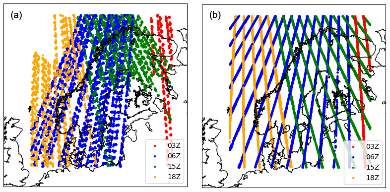
Figure 1Available Aeolus overpasses during the experiment periods: 14 September to 14 October 2018 for laser A (a) and 20 April to 19 May 2020 for laser B (b). The colour indicates the time of the overpass.
In the main part of this paper we use the Harmonie–Arome (cy43) standard data assimilation setup with a three-dimensional variational data assimilation (3D-Var). The data assimilation uses all available conventional observations, aircraft data, and AMSU-A/MHS radiances from polar-orbiting satellites NOAA-18, NOAA-19, MetOp-A, and MetOp-B as well as Aeolus HLOS winds. For the satellite radiance data a variational bias correction (VarBC) based on Dee (2005) and Dee and Uppala (2009) is applied. Background error statistics are calculated from an ensemble of forecast differences (Berre, 2000; Brousseau et al., 2012). These are produced by ensemble data assimilation experiments (EDA; Bonavita et al., 2012) with perturbed observations carried out with the Harmonie–Arome system applying ECMWF global EDA forecasts as lateral boundary conditions. Scaling is applied to the derived statistics in order to be in agreement with the amplitude of Harmonie–Arome +3 h forecast errors. Background and observation errors are assumed to have a Gaussian error distribution as characterized by their error covariances. Observation errors are assumed to be uncorrelated, and their Gaussian distribution within the minimization of the cost function is represented by the error variances. Assumed observation error statistics for all types of observations, except Aeolus HLOS, are static and based on data assimilation studies. The observation-handling main components are the observation operators, which project the model state on the observed quantities, and the background check, which rejects observations assumed to be affected by gross errors and identified by large observation minus background departures. In addition, a thinning is applied to some spatially dense data (such as satellite radiances and aircraft observations) in order to alleviate effects of spatially correlated observation errors not represented in the data assimilation.
The Aeolus HLOS observation operator H consists of a vertical interpolation to the level of the observation, followed by a projection of the model wind field on the horizontal line of sight from the observed position in the direction towards the satellite. An Aeolus HLOS observation, yi, is rejected if it does not satisfy the following inequality:
where σo,i is the observation error standard deviation, σb,i is the background error standard deviation, L is the rejection limit, and [H(xb)]i denotes the projection of the model background state xb on observation i.
The Aeolus product used in this study is the L2B wind product, which provides the HLOS wind speed. This is developed by the ECMWF, KNMI, and the rest of the Aeolus Data, Innovation, and Science Cluster (DISC) team under contract from the ESA. The L2B processing also provides an estimate of the observation instrument noise and corrections for temperature and pressure dependencies of the Rayleigh winds using a priori information from the ECMWF model (Rennie and Isaksen, 2020).
The first set of experiments in this study for laser A was run from 14 September 2018 to 14 October 2018 as recommended by the ESA. ALADIN showed some decay in laser energy over time, and this was a period during which the ESA considered the data quality to be quite good.
In June 2019 the ESA reconfigured ALADIN to use a second available laser, laser B, to improve the data quality, since laser A had degraded in data quality. We have run a second set of experiments focusing on the performance of laser B, starting 20 April 2020 and ending 19 May 2020. This period was chosen because the Aeolus data with M1 temperature-based bias corrections (Rennie and Isaksen, 2020) became available, so the data should have a higher quality than for the previous weeks.
During the second period, Aeolus was used operationally by the ECMWF, so indirectly there will be some influence from Aeolus data in the LBCs for this set of experiments. For all experiments, for both the laser A and the laser B period, the same set of LBCs is used for all parallel experiments. Thus, only the impact from the kilometre-scale limited-area data assimilation of Aeolus data will be investigated in this study. To exploit the impact from the LBC and from the large-scale mixing from introduction of Aeolus data a coordinated experiment with the ECMWF would have been needed, with the ECMWF providing two sets of LBC data with and without assimilation of Aeolus in the ECMWF global model. The use of the same LBC data for both parallel experiments can therefore limit the potential impact we can see from the Aeolus data. The impact of LBC and large-scale mixing vs. regional model data assimilation in Harmonie–Arome is discussed in Randriamampianina et al. (2021).
All the experiments run 3D-Var data assimilation every third hour. The model runs a 12 h forecast at the main cycles at synoptic times (00:00, 06:00, 12:00, 18:00 UTC) and only a 3 h forecast for the remaining cycles. For both periods we run the same set of experiments, namely
-
a reference experiment in which no Aeolus data are assimilated,
-
an experiment assimilating both types of Aeolus data,
-
an experiment assimilating only the Mie data, and
-
an experiment assimilating only the Rayleigh data.
The Aeolus satellite is a research satellite and the first satellite-based wind lidar mission in the world. The HLOS wind observations used in this study are L2B wind products provided by the ECMWF and KNMI, which are suitable for data assimilation in NWP systems (Rennie and Isaksen, 2020). For each Aeolus measurement 20 laser pulses are accumulated, corresponding to a horizontal resolution of approximately 2.9 km. The observations are then made by averaging up to 30 individual measurements for both Rayleigh and Mie channels, which results in horizontally averaged wind data of 86 km. The higher signal-to-noise ratio observed for the Mie channel made it possible to have the horizontal integration length decreased to 12 km. This was implemented in March 2019. To avoid the systematic errors caused by the Rayleigh–Brillouin scattering, corrections are made for the temperature and pressure dependence of Rayleigh data using a priori information from the ECMWF model (Dabas et al., 2008). Moreover, the wind data are retrieved in 24 bins in the vertical in which the resolution varies from 0.25 km near the surface to 2 km at the higher levels. Future investigations concerning the observation collection and processing, as well as how it can be modified to better suit the needs of kilometre-scale regional modelling, are probably needed.
The method used to derive the wind speed data from the raw measurements and the knowledge of how to best use the data in an NWP model are continually under development. Also, the L2B processing software is continuously updated so there are some differences in the processing of the HLOS data for our chosen periods, most notably the correction introduced for the orbital bias caused by the difference in mirror temperature (Rennie and Isaksen, 2020). One aspect that can be improved in future versions of our kilometre-scale data assimilation system is how we handle the different spatial scales represented by the observations and the model. To deal with model noise and spatial representation of observations, a careful evaluation of data assimilation in terms of initializing targeted spatial scales needs further evaluation for the quite different spatial characteristics of the Mie and Rayleigh winds. For example, model noise over the ocean has been demonstrated to be successfully handled by application of a so-called supermodding approach (Mile et al., 2021).
There are some differences in how the HLOS data are assimilated in our Harmonie–Arome experiments. For the first period, with laser A in September–October 2018, we followed the recommendations from the ECMWF (Rennie and Isaksen, 2020) and added a 1.35 m s−1 bias correction to the Mie data. Further, we rejected poor-quality data with large observation errors by specifying an upper limit to the observation error. These limits were set to 4.5 m s−1 for the Mie data and 8 m s−1 for the Rayleigh data. The input data were also limited to one orbit per assimilation window, corresponding to the orbit which had the most observations over the MetCoOp domain.
For the second period, with laser B, the data available for the Mie were of a higher resolution (12 km horizontal distance rather than 86 km as was the case for the laser A period for both the Mie and Rayleigh data). Following our own experience with using Aeolus HLOS data (see Sect. 5.1), we also decided to inflate the observation errors of the Mie data with a factor of 1.25 and also add a lower acceptable limit on the observation error so that all observations with an error lower than 1.5 m s−1 were adjusted upwards to have an observation error of 1.5 m s−1. The upper limit of the observation error of the Mie data was also slightly adjusted and set to 5 m s−1 rather than 4.5 m s−1. For the Rayleigh data all observation errors below 1 m s−1 were set to 1 m s−1, and the upper limit of the observation error for the Rayleigh data was kept at 8 m s−1. All Rayleigh winds below 850 hPa were also rejected due to the poor quality of returned signals in the boundary layer.
The available Aeolus overpasses for the full experiments are shown in Fig. 1; the laser A coverage is shown in the left-hand panel and the laser B coverage is shown in the right-hand panel. The orbits during the laser A period are more irregular than during the laser B period. The higher density of observations of the Mie observations, due to the changes in data sampling during the laser B period, is also seen by the much smaller gaps between the available observations. For both periods, the 06:00 UTC cycle is the cycle that has the most Aeolus observations over the MetCoOp domain.
In order to have a general idea of the performance of the Aeolus HLOS winds over the MetCoOp domain, we studied the difference between the observed values and the model background, which in this case is the 3 h forecast from the previous cycle. In Fig. 2 we show the observation minus background (O − B) statistics, bias, and standard deviation (SD) for both types of HLOS winds compared against the other two sources of wind observations in the upper atmosphere in the experiment, radiosonde, and aircraft data. The bias is close to zero for all the data types in both periods. The only exception is the Rayleigh observations slightly below 400 hPa, which is caused by an undetected “hot pixel” (Fig. 8 Rennie and Isaksen, 2020; Weiler et al., 2020). The standard deviation shows a larger discrepancy between the Aeolus data, both against each other and for the two different periods. Starting with the laser A period, we can see that the Mie data show similar values as the aircraft and radiosonde data, with a standard deviation near 3 m s−1. The Rayleigh data, as expected, show a larger standard deviation of around 4 m s−1. For the laser B period, both the Mie and Rayleigh data quality has worsened. The standard deviation in the Mie data has increased from 3 to 4 m s−1, which is comparable to the Rayleigh values in the laser A period. The accumulation length between the laser A and laser B period was reduced from 86 to 12 km, which increases the signal-to-noise ratio (SNR); this also contributes to the lower accuracy seen in the laser B data. The standard deviation of the Rayleigh data has also increased by nearly 2 m s−1 and there are also larger fluctuations in the vertical profile. This reduced quality of wind data from laser B is caused by the laser's returning energy signal, which was decreasing for this period.
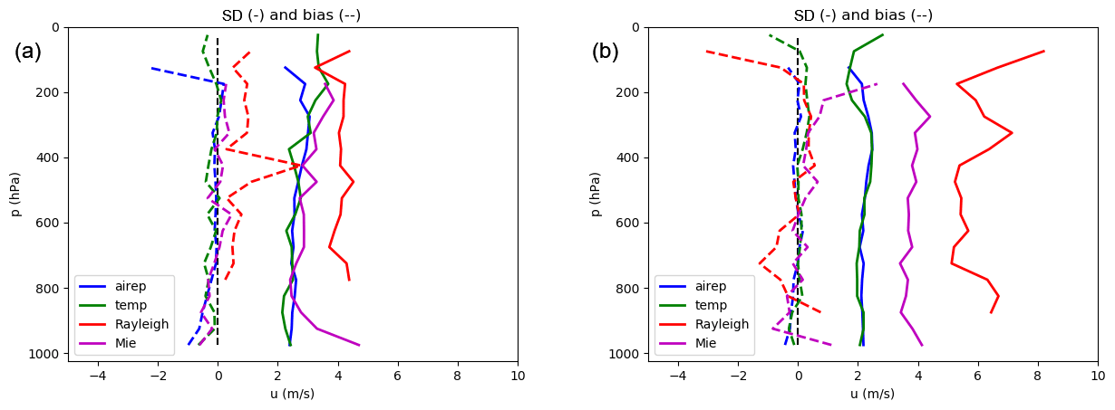
Figure 2The standard deviation and bias of the observation minus background (O − B) for the laser A (a) and laser B (b) periods of Aeolus HLOS data (Rayleigh in red lines and Mie in magenta lines) against aircraft (blue lines) and radiosonde data (green lines).
During these two periods there is also a discrepancy in the availability of upper-air wind observations. For the laser A period, Aeolus observations (both Mie and Rayleigh) correspond to 14 % of the total wind observations in the upper air, with the rest of the data coming from radiosondes (35 %) and aircraft measurements (51 %). For the laser B period, in the spring of 2020 there were considerably fewer aircraft observations available due to the limited number of flights during this period because of travel restrictions brought in as a measure against the Covid-19 situation. For this period there are as many Aeolus observations as there are aircraft observations; both types of data make up 37 % of the total number of observations, and radiosonde data make up the remaining 26 % of upper-air wind observations.
In the early period of the Aeolus satellite there were reports of discrepancy in the bias depending on the direction of travel of Aeolus (Rennie and Isaksen, 2020; Martin et al., 2020). Over the MetCoOp domain the HLOS observations available at 03:00 and 06:00 UTC come from the descending part of the orbit (the satellite is travelling southward) and the observations at 15:00 and 18:00 UTC are from the ascending phase of the orbit (satellite travelling northwards). In Fig. 3 we show the bias of the O − B values for ascending and descending orbits for both periods for both Mie (left) and Rayleigh (right). The top row shows the O − B statistics for the laser A period (September–October 2018); for the bias a clear difference between the descending and ascending orbits can be seen in both Mie and Rayleigh data. There is a much smaller difference in the standard deviation; the Mie data have a smaller standard deviation for ascending orbits, whereas for the Rayleigh data the descending orbits have a smaller standard deviation. The same comparison for the laser B period (April–May 2020) does not show the same difference in bias for ascending and descending orbits, except for the very lowest level of Rayleigh data. The differences in standard deviation are also much lower, particularly for the Rayleigh data. If the bias identified in the laser A period cannot be solved by a future refined reprocessing of the observations one could consider introducing an adaptive variational bias correction (Dee, 2005) for the Aeolus HLOS data.

Figure 3The bias and standard deviation of the observation minus background (O − B) for the laser A (a, b) and laser B (c, d) periods of Aeolus HLOS data. The Mie data are in the left-hand column, and the Rayleigh data are in the right-hand column. Blue lines mark ascending orbits and red lines descending ones. The black dotted line shows the respective number of Aeolus observations.
4.1 Impact on analyses
A first step to understanding the impact that Aeolus data have on our NWP system is to compare the observation minus background (O − B) statistics with the observation minus analysis (O − A) values. The upper panels of Fig. 4 show the difference between O − B and O − A departures for both types of HLOS data and for both periods. The lower panels of Fig. 4 show mean specified observation error standard deviations for Mie and Rayleigh data for the two periods and also corresponding estimated background error standard deviations. There is a clear difference between O − B and the O − A standard deviation for both Mie and Rayleigh data, meaning that the Aeolus observations have an impact on the upper-air initial states of the NWP system. The Mie data, with smaller observation errors, adjust the initial state more than the Rayleigh data for both periods. The exact deviation between O − A and O − B is also influenced by the magnitude of the standard deviations of the background error equivalents and the influences from other types of observations. There is a clear difference in average observation error (bottom half, Fig. 4) between the two periods. Average observation errors are larger for both Mie and Rayleigh data during the laser B period. This is also reflected in the larger O − B and O − A standard deviations for the laser B period than for the laser A period. It should be noted that the departure statistics presented here mainly provide information on the observation quality and influence of the data on the initial states. Information on the impact on actual forecast quality is limited.

Figure 4Standard deviations of O − B (solid lines) and O − A (dashed lines) departures for Mie (blue) and Rayleigh (red) observations during the laser A period (a) and laser B period (b). The mean observation errors for the same data are shown in the lower half of the figure, together with the background error (black dashed lines).
Another way to investigate the impact of the Aeolus data on the Harmonie–Arome model initial state is to calculate the degree of freedom of signal (DFS). DFS is the derivative of the analysis increments in observation space with respect to the observations used in the analysis system and can be calculated using a randomization technique as proposed by Chapnik et al. (2006). This has the advantage that the total impact of all Aeolus HLOS observations on the initial state can be estimated and compared with the impact of other observation types. The absolute DFS represents the information brought into the analyses by the different observation types in terms of number, distribution, estimated instrumental accuracy, and observation operator definition. It provides information on the weight given to all observations of one particular type within the analysis system. There is also a possibility of estimating the DFS per observation through calculation of relative DFS by normalizing the absolute DFS by the number of observations belonging to one particular type of observation (Randriamampianina et al., 2011). The information obtained with relative DFS is comparable with O − B and O − A statistics.
Figure 5 shows the DFS of all wind observations used in the data assimilation, SYNOP, radiosonde, and aircraft data as well as Aeolus data. The column to the left shows the DFS for all Aeolus data; the middle one is for the Mie data, and the right-hand one is for Rayleigh data. This DFS calculation is done using all cycles of the day and for all cycles with Aeolus data every fifth day of the experiment period, which for the figure shown is the laser B period. The reason for using cycles from every fifth day is to use independent weather situations in the DFS statistics. The DFS clearly shows that for the Aeolus data the relative impact (bottom row) is significantly larger than the absolute impact (top and middle rows). This is an indication that a relatively large weight is given to the Aeolus HLOS observations and that there are rather few Aeolus HLOS observations. The relative DFS shown in the lower panels of the middle and right columns show, consistent with Fig. 4, that a larger weight is given to the Mie observations than to the Rayleigh observations. It should be kept in mind that large relative DFS is not necessarily a good thing and the results should be interpreted with care since it might be an indication of overfitting of observations, which might have detrimental effects on forecast quality. In our case the observation and background errors have, however, been carefully studied with the Desroziers approach and with a restrictive position on reducing the observation error compared with the model background equivalent. From the corresponding upper panels in Fig. 5 it is evident that despite fewer observations, Mie observations have a larger influence on initial state than the Rayleigh observations, and the Mie data have the largest relative impact of all the observations. The Rayleigh data on their own also have a larger relative than absolute impact on the DFS values, but their relative importance is the smallest of the four observation types instead of the largest. When using all Aeolus data, the relative DFS of the Aeolus data is equal to that from the radiosonde data, which has the largest absolute DFS value. If we repeat the DFS calculation, but only use the cycles for the same set of days when there are Aeolus observations (top row Fig. 5), the absolute DFS for Aeolus increases. In two cases (all Aeolus data and Mie only) it has the third-largest DFS of the four observation types.
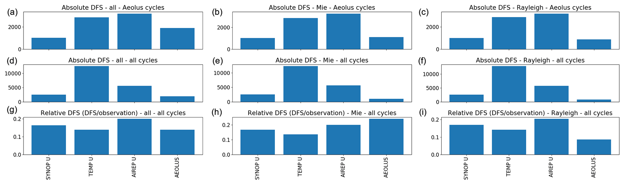
Figure 5Degree of freedom of signal (DFS) for the experiment with all Aeolus data (a, d, g), only Mie data (b, e, h), and only Rayleigh data (c, f, i) for the laser B period compared with other sources of wind data. The absolute DFS for all cycles with Aeolus data is shown in the top row; the middle row shows the absolute DFS for all cycles, and the relative DFS for all cycles is shown in the bottom row.
4.2 Impact on forecasts
To verify the wind forecast, we compare it to radiosonde data. These are available twice per day, and in the MetCoOp domain we can find up to 18 radiosonde stations. Because of the different availability times of the radiosonde and Aeolus HLOS observations, only some of the forecasts which are analysed in this section start from a data assimilation wherein Aeolus HLOS data have been used. In order to see as much impact of the Aeolus data as possible, we verify the forecasts after 6 h so that as far as possible the forecasts will have started from a data assimilation which contained Aeolus data. The forecasts starting at 06:00 and 18:00 UTC will generally have used Aeolus data in the data assimilation, but this is not the case for all as the Aeolus satellite track changes. The 6 h forecasts from these cycles will be valid at 12:00 and 00:00 UTC and are verified against the radiosonde data.
The error standard deviation of the wind speed and direction for the 6 h forecasts for both periods for four different set-ups (no Aeolus data – Ref, Mie only, Rayleigh only, and both Mie and Rayleigh) is shown in Fig. 6. For the laser A period we can see a small improvement in the SD of the wind speed for the Mie-only experiment below 800 hPa. At 800 hPa there is also a small improvement in the SD of the wind direction. For the laser B period the verification shows the worst wind speed SD values for the Mie-only experiment, whereas the best SD for the wind direction below 500 hPa is also seen in the Mie-only experiment. Overall the impact of using Aeolus data is mostly neutral. The impact on other variables, such as temperature and pressure, is neutral for all experiments.
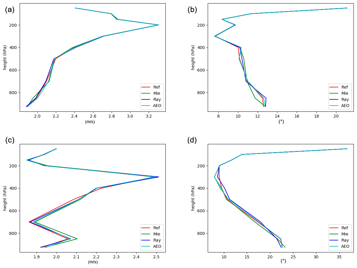
Figure 6The error standard deviation of the wind speed (a, c) and wind direction (b, d) for the laser A period (a, b) and laser B period (c, d) for the 6 h forecast valid at 00:00 and 12:00 UTC. The experiment without Aeolus data is shown in red, the Mie only in green, the Rayleigh only in blue, and the experiment using both Mie and Rayleigh in cyan. Note the different sizes of the x axis.
The bias of the wind speed for the 6 h forecast for this set of experiments (not shown) is around −0.2 m s−1 for all experiments, and periods with the largest bias (−0.4 m s−1) are found at 400 hPa of height. The differences in bias between the different experiments are very small and vary with height in terms of which experiment shows the lowest value of the bias. In general the wind speed bias is between 0 and −0.4 m s−1 for laser A and between 0.1 and −0.5 m s−1 for laser B. The bias for the wind direction varies with height, and a negative bias is found near the surface and for the higher vertical heights.
We also looked at the O − B statistics for aircraft data for the cycles wherein Aeolus data were used by the background forecast to investigate the quality of the 3 h forecast. As expected, the large-scale mixing smoothed out the results, and the resulting SD of O − B is neutral when comparing the Mie-only and Rayleigh-only experiment to the control forecast (without Aeolus data in the assimilation). This investigation was only conducted for the laser B experiment, but we anticipate that it would give a similar result for the laser A data.
The impact on the forecast verification of using Aeolus data in the data assimilation was neutral for the other meteorological parameters for both the laser A and laser B periods.
5.1 Tuning of error statistics in the present assimilation system
Following the method described by Desroziers et al. (2005), we analysed the observation and background errors for the experiment actively assimilating the Aeolus HLOS winds. The result is shown by the solid lines in Fig. 7. This method is limited by the fact that it assumes that the background error and observation error covariances are correctly specified. With this in mind, running the Desroziers diagnostics for our results shows that the wind speed background errors (red solid lines) are smaller than wind speed observation errors for Aeolus (black solid lines). The estimation of the optimal values of these two parameters using the Desroziers method shows that while the background values should still be more trusted than the observations, both of them are trusted too much and should be given less weight since the estimated values of σB and σO are larger than the ones that are used by the model. The importance of a proper representation of σB values in limited-area model data assimilation has been studied by Lindskog et al. (2006). They found a positive impact on average verification scores and that, in addition, a substantial positive impact is demonstrated for an individual synoptically active case by adjusting the observation error.

Figure 7(a) The mean standard deviation of the background error (σB, red line) and the observation error (σO, black) used by the data assimilation and the estimated values of σB (blue) and σO (green) from the Desroziers diagnostics. The settings for the updated data assimilation are drawn with dashed lines. (b) The ratio between what was used (blue solid line) and the estimated ratio (green solid line) as well as the ratio used in the experiment with updated settings (blue dashed line).
A new experiment was run in which the background error is increased (the background is less trusted)1 and the observation errors were also changed. A previous experiment used the observation errors as reported in the Aeolus data themselves. Since the Desroziers diagnostic also indicated that the observations were given a too much weight, we manually changed all observation errors under 1.5 m s−1 so that they were considered by the data assimilation system to have a 1.5 m s−1 observation error and thus given less weight in the data assimilation process. In another experiment we tested manually lowering the upper observation error as well, but this experiment showed us that the higher observation errors should be trusted and that artificially lowering them decreased the forecast skill.
The new values of σB and σO are shown on the left-hand side of Fig. 7 in dashed lines, comparing them to the original values (in the same colours but with solid lines). We have increased the error more for the background than for the observations because the σO will also have an impact on the other observations used in the data assimilation. The goal is that the ratio of σB and σO of the values used should also be close to what is estimated by the Desroziers diagnostics. Below 400 hPa this is achieved (blue dashed line in Fig. 7, right), but between 400 and 100 hPa, the ratio of the updated settings is smaller than the recommended value.
An experiment using the updated settings indicated by the Desroziers diagnostics was run for the full laser A period, and it resulted in similar O − B as the reference experiment but smaller O − A values (not shown) by on average 0.45 m s−1 SD. This means that overall the observations have been given more weight in the data assimilation and thus influence the analysis more. Looking at the verification scores, the impact of the change in background and observation error settings is neutral.
In order to investigate whether there was a difference between the two types of HLOS observations, we ran the Desroziers diagnostic for the two experiments assimilating only Mie or only Rayleigh winds. These showed that the Desroziers diagnostic recommended a larger increase in the σO for the Mie-only experiment than what was shown by the same diagnostics when run for the Rayleigh-only experiment. Taking these results into account when running the laser B experiments, we decided to inflate the observation errors for the Mie observations.
We also ran the Desroziers diagnostics for the laser B period for the experiment assimilating both Mie and Rayleigh data from Aeolus. Again the diagnostics recommended an increase in the background and observation errors, though both suggested increases were smaller than the ones derived from the laser A period. Since the laser B experiment used the default setting for the background error, it is not obvious why the recommended increase by the Desroziers diagnostic is smaller. It is easier to understand why the increase recommended for the observation error was smaller, since this was already increased for the Mie observations in the laser B experiment due to the shorter accumulation length (see Sect. 3).
5.2 Refined data assimilation technique
The potential for enhanced use of Aeolus HLOS wind observations by application of an enhanced data assimilation technique has been exploited. This was achieved within a single observation data assimilation framework in which the currently used 3D-Var method was compared with a four-dimensional variational data assimilation (4D-Var; Courtier et al., 1994) framework. Two main advantages of 4D-Var compared to 3D-Var are that observations are used at their appropriate time and that (a simplified version of) the forecast model is used when minimizing the penalty function (Gustafsson et al., 2012). The latter implies a flow dependency of data assimilation corrections of the background, which has a clear potential advantage for Aeolus HLOS data assimilation. As described by Gustafsson et al. (2018) data assimilation is less developed for kilometre-scale models than for the meso-beta-scale models. Nevertheless, a four-dimensional variational data assimilation methodology has been developed for the Harmonie–Arome kilometre-scale forecasting system and has the potential to further enhance the use of observations.
The single Aeolus HLOS observation parallel 3D-Var/4D-Var experiment was designed for the data assimilation cycle on 25 May 2020 at 06:00 UTC. 3D-Var is designed to have a 3 h data assimilation time window extending from 04:30 to 07:30 UTC. The present 4D-Var version is designed to have a 2 h data assimilation window starting at 05:00 UTC and ending at 07:00 UTC. The background state for 3D-Var is a 3 h forecast produced from a Harmonie–Arome initial state valid on 25 May 2020 at 03:00 UTC. The background state for 4D-Var is a 2 h forecast produced from the initial state valid on 25 May 2020 at 03:00 UTC. The 3D-Var initial state is computed at 06:00 UTC by minimizing a penalty function. The equivalent 4D-Var initial state at 06:00 UTC is produced by generating an initial state valid at 05:00 UTC, followed by a non-linear propagation of the increments to 06:00 UTC. From the 3D-Var- and 4D-Var-generated analyses valid at 06:00 UTC, forecasts can be launched. The single simulated Aeolus HLOS observation is on 25 May 2020 at 06:50 UTC. It is located at 65.3∘ latitude, 15.0∘ longitude, and at a vertical level of 679 hPa. The simulated Aeolus HLOS observation was from an ascending satellite orbit (north to south) and with the instrument looking in a direction approximately towards the west. With this configuration a westerly observed wind gives a negative Aeolus HLOS observation (positive direction defined to be for the wind direction away from the lidar, and the negative direction is towards the lidar). Here the observed value is −7.0 m s−1, with an assigned observation error standard deviation of approximately 0.7 m s−1. This corresponds to an accurate Mie Aeolus HLOS observation.
The 3D-Var background wind field at model levels around 3 km as well as the wind and temperature fields at 10 km are shown together with the location of the single Aeolus HLOS observation in Fig. 8. A frontal structure is evident along the Swedish–Norwegian border with sharp gradients and an approximate north–south flow along the front line. The single observation (marked with a dot) was positioned slightly east of the frontal area and valid 50 min after the valid time of the 3D-Var background state.
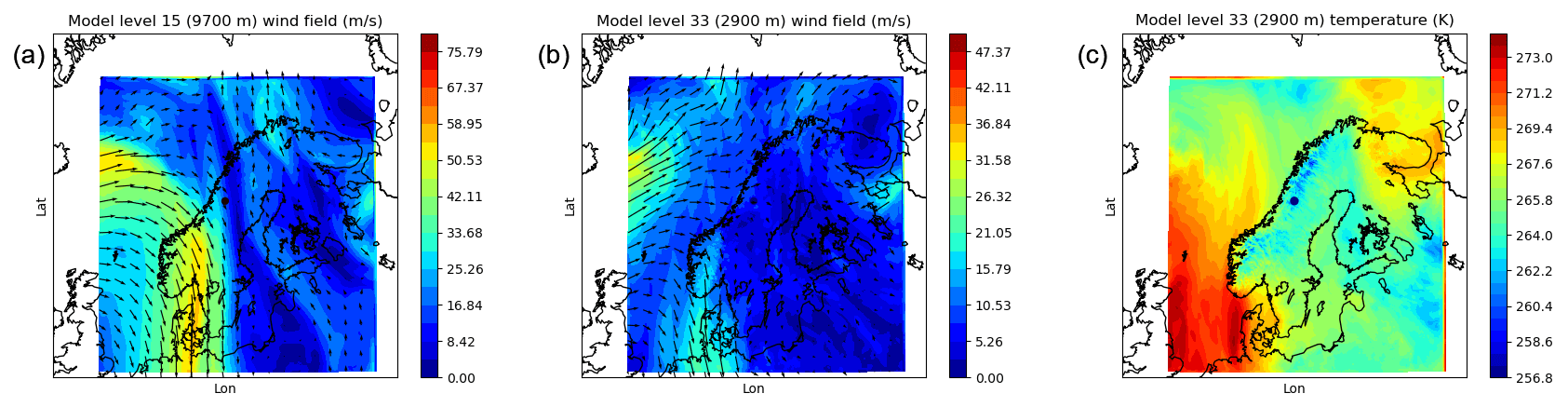
Figure 8Wind (a, b) and temperature (c) field of +3 h forecast launched on 25 May 2020 at 03:00 UTC and valid on 25 March 2020 at 06:00 UTC. Also shown is the horizontal location of a single Aeolus HLOS observation with a dot.
In Fig. 9 the horizontal wind field assimilation increments at 06:00 UTC for model level 33 (around 3 km) induced by the single Aeolus HLOS simulated observation is shown for 3D-Var (left) and 4D-Var (right). An important difference between 3D-Var- and 4D-Var-induced increments is that 3D-Var increments have a considerably larger magnitude than the 4D-Var increments. Furthermore, the 4D-Var increments have a smaller spatial scale and they are more flow-dependent than the 3D-Var increments. This flow dependency is evident in small-scale variations due to the flow over a mountainous region and also due to a more north–south component of the 4D-Var increments, in agreement with the flow of the background state. This enhanced flow dependency is due to the utilization of the forecast model within the 4D-Var assimilation procedure. The main reason for the large difference in magnitude of assimilation increments between 3D-Var and 4D-Var is that with 4D-Var the observation is compared with a background model equivalent valid at 06:50 UTC, while with 3D-Var the observation is compared with a model equivalent valid at 06:00 UTC. In this highly flow-dependent case with large wind increments this will result in 3D-Var observation minus background departures of −2.3 m s−1 and in 4D-Var observation minus background departures of −0.5 m s−1.
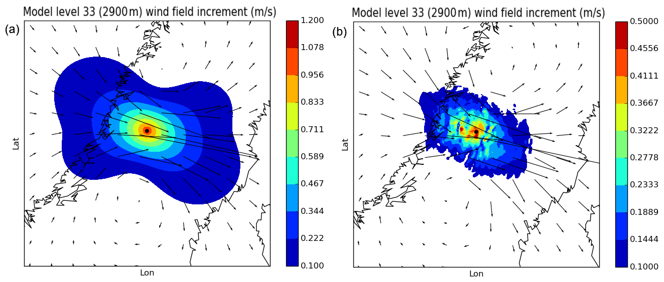
Figure 9Model level 33 (around 3 km) 3D-Var (a) and 4D-Var (b) analysis increments on 25 May 2020 at 06:00 UTC, with resulting Aeolus HLOS observation (position marked with a dot). Please note the difference in colour scale used for the two panels.
The idealized Aeolus HLOS single-observation study has indicated that there can be a clear benefit in the use of Aeolus HLOS observations from application of more flow-dependent and advanced assimilation technique taking the exact time of the observations into better account, and it also should make better use of the model within the data assimilation process.
Aeolus HLOS wind profiles have been added to the 3D-Var data assimilation in a regional high-resolution NWP system. In this study we have used the Harmonie–Arome model running over the MetCoOp domain covering the Nordic countries. We have used the assimilation system to investigate the quality of the Aeolus satellite winds for two different 4-week periods, one early in the life of the satellite in September–October 2018 and the other after more than 2 years of operations in April–May 2020, and the impact of the Aeolus data on the Harmonie–Arome NWP system has been investigated.
We conclude that Aeolus Mie data are demonstrated to be of considerably higher quality and more suitable for assimilation in our regional kilometre-scale forecasting system than Rayleigh data during the two periods we studied. The Mie data are of a quality comparable to radiosonde and aircraft observations for the laser A period, while Rayleigh has a lower quality. For the laser B period, even though the Mie quality is lower with respect to the laser A period, it still has the same relative higher quality compared to the Rayleigh data. Another difference in the Mie data between the laser A and the laser B period is the decrease in accumulation length from 86 km to nearer 12 km.
We have shown that the Aeolus data have an impact on the analysis as seen in the difference between O − B and O − A SD profiles as well as through DFS analysis. From the DFS analysis we see that the Mie data have a larger impact on the analysis than the Rayleigh data and that the relative impact of the Aeolus data is larger than the absolute impact. Given that the information content from the Aeolus data, as seen in the absolute DFS, is small relative to the other sources of upper-air data it is not unexpected that the Aeolus data have a mostly neutral impact on the verification of forecasts, with some small improvements seen in the wind speed and direction at selected height intervals. For the laser A period we noticed somewhat better verification scores if using Mie data only. This result is consistent with the analysis of the quality of Aeolus data. In future analyses of the impact of Aeolus observations we would also like to investigate the impact on the two wind components.
Different approaches for further enhancing the impact of Aeolus data by new adoptions of the Harmonie–Arome data assimilation system were investigated. Such enhancements concerned tuned error statistics and application of a refined flow-dependent assimilation technique. Results from analysis of error statistics based on the Desroziers approach indicated that potential optimizations of currently used error statistics concerning Aeolus could be carried out. Application of such modifications resulted in a rather neutral impact on forecast quality. Clear potential was, however, seen using a 4D-Var assimilation technique, allowing for taking the actual time of the observation into better account and using the forecast model itself within the assimilation process.
All in all, we have found that the Aeolus data have a small impact on the Harmonie–Arome forecast. However, there are some small positive changes to the analysis which can be seen in the O − A and O − B statistics. As proposed by Stoffelen et al. (2020), having several Doppler wind lidar instruments in orbit and thus more overpasses would be more beneficial as we would have more data available, potentially for all our forecast cycles.
In the future, it would also be interesting to use the reprocessed data for the laser A period and rerun these experiments in order to conduct a deeper analysis of the impact of the resolution, both vertical and horizontal, vs. observation quality in our regional model. It would also be interesting to more fully examine the potential improvement in the impact of Aeolus data on both analyses and forecasts if 4D-Var data assimilation is used for a longer trial. In addition, it would be fruitful to coordinate the study with an ECMWF Aeolus experiment to fully exploit the impact of Aeolus from regional data assimilation, LBC, and large-scale mixing. Moreover, in this study we mainly focused on observation error standard deviations, whereas potential observation error correlations would be a subject for future studies.
Another aspect that can be improved in future versions of our kilometre-scale data assimilation system is how we handle the fact that observations and the model represent different spatial scales. In the case of observations representing courser spatial scales than the model this scale difference has been demonstrated to be successfully handled by application of a so-called supermodding approach (Mile et al., 2021).
The ACCORD consortia cooperate on the development of a shared system of model codes. The Harmonie–Arome model is part of the ACCORD system, and all members are allowed to licence the Harmonie–Arome code within their home country for non-commercial research. Access to the codes can be obtained by contacting one of the member institutes (http://www.accord-nwp.org/?Members, last access: 1 June 2020) (ACCORD, 2020).
The Aeolus observation data can be downloaded from https://earth.esa.int/eogateway/missions/aeolus/data (ESA, 2021).
SH is the main author and, together with RA, was responsible for running the experiments and performing data analysis. RA also provided input on the paper and contributed to the 4D-Var experiment. ML is responsible for the 4D-Var experiments and wrote part of the paper. HS and HK contributed to the writing of the paper.
The authors declare that they have no conflict of interest.
Publisher's note: Copernicus Publications remains neutral with regard to jurisdictional claims in published maps and institutional affiliations.
This article is part of the special issue “Aeolus data and their application (AMT/ACP/WCD inter-journal SI)”. It is not associated with a conference.
SMHI was funded by Rymdstyrelsen (Swedish National Space Agency) Dnr 279/18. Met Norway was funded by the ESA (European Space Agency) PRODEX (PROgramme de Développement d'Expériences scientifiques) programme.
This paper was edited by Ad Stoffelen and reviewed by three anonymous referees.
Anderson, E. and Sato, Y. (Eds.): Fifth WMO Workshop on the Impact of Various Observing Systems on NWP, Sedona, Arizona, USA, 22–25 May 2012, WMO, 2012. a
A Consortium for Convection-scale modelling Research and Development (ACCORD): NWP model code, ACCORD [code], available at: http://www.accord-nwp.org/?Members, last access: 1 June 2020. a
Bengtsson, L., Andrae, U., Aspelien, T., Batrak, Y., Calvo, J., de Rooy, W., Gleeson, E., Hansen-Sass, B., Homleid, M., Hortal, M., Ivarsson, K.-I., Lenderink, G., Niemelä, S., Nielsen, K. P., Onvlee, J., Rontu, L., Samuelsson, P., Muñoz, D. S., Subias, A., Tijm, S., Toll, V., Yang, X., and Køltzow, M. O.: The HARMONIE-AROME Model Configuration in the ALADIN-HIRLAM NWP System, Mon. Weather Rev., 145, 1919–1935, https://doi.org/10.1175/MWR-D-16-0417.1, 2017. a, b
Berre, L.: Estimation of synoptic and meso scale forecast error covariances in a limited area model, Mon. Weather Rev., 128, 664–667, 2000. a
Bonavita, M., Isaksen, L., and Holm, E.: On the use of EDA background error variances in the ECMWF 4D Var, Q. J. Roy. Meteor. Soc., 138, 1540–1559, https://doi.org/10.1002/qj.1899, 2012. a
Brousseau, P., Berre, L., Bouttier, F., and Desroziers, G.: Flow-dependent background-error covariances for a convective-scale data assimilation system, Q. J. Roy. Meteor. Soc., 138, 310– 322, https://doi.org/10.1002/qj.920, 2012. a
Chapnik, B., Desroziers, G., Rabier, F., and Talagrand, O.: Diagnosis and tuning of observational error in a quasi-operational data assimilation setting, Q. J. Roy. Meteor. Soc., 132, 543–565, 2006. a
Courtier, P., Thépaut, J.-N., and Hollingsworth, A.: A strategy for operational implementation of 4D-Var using an incremental approach, Q. J. Roy. Meteor. Soc., 120, 1367–1388, 1994. a
Dabas, A., Denneulin, M., Flamant, P., Loth, C., Garnier, A., and Dolfi-Bouteyre, A.: Correcting winds measured with a Rayleigh Doppler lidar from pressure and temperature effects, Tellus, 60A, 206–215, https://doi.org/10.1111/j.1600-0870.2007.00284.x, 2008. a
Dee, D.: Bias and data assimilation, Q. J. Roy. Meteor. Soc., 131, 3323–3343, 2005. a, b
Dee, D. and Uppala, S.: Variational bias correction of satellite radiance data in the ERA-Interim reanalysis, Q. J. Roy. Meteor. Soc., 135, 1830–1841, 2009. a
Desroziers, G., Berre, L., Chapnik, B., and Poli, P.: Diagnosis of observation, background and analysis-error statistics in observation space, Q. J. Roy. Meteor. Soc., 131, 3385–3396, https://doi.org/10.1256/qj.05.108, 2005. a
European Space Agency (ESA): Aeolus Data, available at: https://earth.esa.int/eogateway/missions/aeolus/data (last access: 1 June 2020), 2021. a
Geer, A. J., Baordo, F., Bormann, N., Chambon, P., English, S. J., Kazumori, M., Lawrence, H., Lean, P., Lonitz, K., and Lupu, C.: The growing impact of satellite observations sensitive to humidity, cloud and precipitation, Q. J. Roy. Meteor. Soc., 143, 3189–3206, https://doi.org/10.1002/qj.3172, 2017. a
Gustafsson, N., Huang, X.-Y., Yang, X., Mogensen, K., Lindskog, M., Vignes, O., Wilhelmsson, T., and Thorsteinsson, S.: Four-dimensional variational data assimilation for a limited area model, Tellus A, 64, 14985, https://doi.org/10.3402/tellusa.v64i0.14985, 2012. a
Gustafsson, N., Janjic, T., Schraff, C., Leuenberger, D., Weissmann, M., Reich, H., Brousseau, P., Montmerle, T., Wattrelot, T., Bučánek, A., Mile, M., Hamdi, R., Lindskog, M., Barkmeijer, J., Dahlbom, M., Macpherson, B., Ballard, S., Inverarity, G., Carley, J., Alexander, C., Dowell, D., Liu, S., Ikuta, Y., and Fujita, T.: Survey of data assimilation methods for convective-scale numerical weather prediction at operational centres, Q. J. Roy. Meteor. Soc., 144, 1218–1256, https://doi.org/10.1002/qj.3179, 2018. a
Halloran, G.: Assessment and assimilation of L2B winds at the Met Office, in: Aeolus cal/val virtual workshop, 2–6 November 2020, available at: https://www.dropbox.com/s/4vh02bq7wy3snio/Gemma_Halloran_Oral_AssessmentandAssimilationMetOffice.pdf?dl=0 (last access: 30 August 2021), 2020. a
Lindskog, M., Gustafsson, N., and Mogensen, K.: Representation of background error standard deviations in a limited area model data assimilation system, Tellus, 58A, 430–444, 2006. a
Martin, A., Weissmann, M., Reitebuch, O., Rennie, M., Geiß, A., and Cress, A.: Validation of Aeolus winds using radiosonde observations and numerical weather prediction model equivalents, Atmos. Meas. Tech., 14, 2167–2183, https://doi.org/10.5194/amt-14-2167-2021, 2021. a, b, c
Mile, M., Randriampianina, R., Marseille, G.-J., and Stoffelen, A.: Supermodding – A special footprint operator for mesoscale data assimilation using scatterometer winds, Q. J. Roy. Meteor. Soc., 147, 1382–1402, https://doi.org/10.1002/qj.3979, 2021. a, b
Müller, M., Homleid, M., Ivarsson, K.-I., Køltzow, M. A. O., Lindskog, M., Midtbø, K. H., Andrae, U., Aspelien, T., Berggren, L., Bjørge, D., Dahlgren, P., Kristiansen, J., Randriamampianina, R., Ridal, M., and Vignes, O.: AROME-MetCoOp: A Nordic Convective-Scale Operational Weather Prediction Model, Weather Forecast., 32, 609–627, https://doi.org/10.1175/WAF-D-16-0099.1, 2017. a
Pourret, V., Savli, M., Mahfouf, J.-F., Raspaud, D., Doerenbecher, A., Bénichou, H., and Payan, C.: Operational assimilation of Aeolus winds in the Météo-France global NWP model ARPEGE, Q. J. Roy. Meteor. Soc., in preparation, 2021. a
Randriamampianina, R., Iversen, T., and Storto, A.: Exploring the assimilation of IASI radiances in forecasting polar lows, Q. J. Roy. Meteor. Soc., 137, 1700–1715, https://doi.org/10.1002/qj.838, 2011. a
Randriamampianina, R., Bormann, N., Køltzow, M. A. O., Lawrence, H., Sandu, I., and Wang, Z. Q.: Relative impact of observations on a regional Arctic numerical weather prediction system, Q. J. Meteor. Soc., 147, 2212–2232, https://doi.org/10.1002/qj.4018, 2021. a
Reitebuch, O., Lemmerz, C., Nagel, E., Paffrath, U., Durand, Y., Endemann, M., Fabre, F., and Chaloupy, M.: The Airborne Demonstrator for the Direct-Detection Doppler Wind Lidar ALADIN on ADM-Aeolus. Part I: Instrument Design and Comparison to Satellite Instrument, J. Atmos. Ocean. Tech., 26, 2501–2515, https://doi.org/10.1175/2009JTECHA1309.1, 2009. a
Rennie, M. P. and Isaksen, L.: The NWP impact of Aeolus Level 2B winds at ECMWF, ECMWF technical memo, 864, 2020. a, b, c, d, e, f, g
Šavli, M., Žagar, N., and Anderson, J. L.: Assimilation of horizontal line of sight winds with a mesoscale EnKF data assimilation system, Q. J. Roy. Meteor. Soc., 144, 2133–2155, https://doi.org/10.1002/qj.3323, 2018. a
Simmons, A. J. and Hollingsworth, A.: Some aspects of the improvement in skill of numerical weather prediction, Q. J. Roy. Meteor. Soc., 128, 647–677, https://doi.org/10.1256/003590002321042135, 2002. a
Skamarock, W., Klemp, J., Dudhi, J., Gill, D., Barker, D., Duda, M., Huang, X., Wang, W., and Powers, J.: A Description of the Advanced Research WRF Version 3, Technical Note, TN 475 STR, 2008. a
Stoffelen, A., Pailleux, J., Källén, E., Vaughan, J. M., Isaksen, L., Flamant, P., Wergen, W., Andersson, E., Schyberg, H., Culoma, A., Meynart, R., Endemann, M., and Ingmann, P.: The atmospheric dynamics mission for global wind field measurement, B. Am. Meteorol. Soc., 86, 73–88, https://doi.org/10.1175/BAMS-86-1-73, 2005. a
Stoffelen, A., Benedetti, A., Borde, R., Dabas, A., Flamant, P., Forsythe, M., Hardesty, M., Isaksen, L., Källén, E., Körnich, H., Lee, T., Reitebuch, O., Rennie, M., Riishøjgaard, L.-P., Schyberg, H., Straume, A. G., and Vaughan, M.: Wind profile satellite observation requirements and capabilities, B. Am. Meteorol. Soc., 101, E2005–E2021, https://doi.org/10.1175/BAMS-D-18-0202.1, 2020. a
Weiler, F., Kanitz, T., Wernham, D., Rennie, M., Huber, D., Schillinger, M., Saint-Pe, O., Bell, R., Parrinello, T., and Reitebuch, O.: Characterization of dark current signal measurements of the ACCDs used on board the Aeolus satellite, Atmos. Meas. Tech., 14, 5153–5177, https://doi.org/10.5194/amt-14-5153-2021, 2021. a
This is done by changing the value of the REDNMC variable, which is set to 0.6, representing a decrease from its original value of 1.0.
- Abstract
- Introduction
- Description of the NWP model and study choice
- Characteristics of Aeolus data
- Impact on the NWP system
- Potential for enhanced use of Aeolus data
- Conclusions
- Code availability
- Data availability
- Author contributions
- Competing interests
- Disclaimer
- Special issue statement
- Financial support
- Review statement
- References