Calibration and assessment of electrochemical low-cost sensors in remote alpine harsh environments

This work presents results from an original open-source low-cost sensor (LCS) system developed to measure tropospheric O₃ in a remote high altitude alpine site. Our study was conducted at the Col Margherita Observatory (2543 m above sea level), in the Italian Eastern Alps. The sensor system mounts three commercial low-cost ${\mathrm{O}}_{\mathrm{3}}/{\mathrm{NO}}_{\mathrm{2}}$ sensors that have been calibrated before field deployment against a laboratory standard (Thermo Scientific; 49i-PS), calibrated against the standard reference photometer no. 15 calibration scale of the World Meteorological Organization (WMO). Intra- and intercomparison between the sensors and a reference instrument (Thermo Scientific; 49c) have been conducted for 7 months from May to December 2018. The sensors required an individual calibration, both in laboratory and in the field. The sensor's dependence on the environmental meteorological variables has been considered and discussed. We showed that it is possible to reduce the bias of one LCS by using the average coefficient values of another LCS working in tandem, suggesting a way forward for the development of remote field calibration techniques. We showed that it is possible reconstruct the environmental ozone concentration during the loss of reference instrument data in situations caused by power outages. The evaluation of the analytical performances of this sensing system provides a limit of detection (LOD) <5 ppb (parts per billion), limit of quantification (LOQ) <17 ppb, linear dynamic range (LDR) up to 250 ppb, intra-Pearson correlation coefficient (PCC) up to 0.96, inter-PCC >0.8, bias >3.5 ppb and ±8.5 at 95 % confidence. This first implementation of a LCS system in an alpine remote location demonstrated how to obtain valuable data from a low-cost instrument in a remote environment, opening new perspectives for the adoption of low-cost sensor networks in atmospheric sciences.

1 Introduction

The troposphere is a very complex system which is subject to continuous inputs, production and removal processes of ozone from natural phenomena and human activities (lifetime ∼ 25 d; Young et al., 2013). In southern Europe, the background tropospheric ozone concentration appears to be significantly affected by three main air mass transport processes, namely the (i) transport of polluted air masses on regional and long-range scales, (ii) downward transport of stratospheric air masses and (iii) transport of mineral dust (Cristofanelli and Bonasoni, 2009). Large gaps remain in the surface observation network, despite many years of research and monitoring of surface ozone on regional and global scales, especially in terms of areas without monitoring and in terms of regions that have monitoring programmes but no public access to the data archive (Schultz et al., 2017). Future improvements in the database would require better data harmonisation, enhanced data sharing and monitoring in data sparse regions to develop and integrate in situ networks, complementary to satellite instruments, in order to improve measurement accuracy and spatiotemporal sampling (O'Neill et al., 2015). Therefore, covering in situ spatial data gaps to increase the effectiveness of satellite observations, which must be calibrated using ground-based reference measurements (WMO-GAW, 2017), is necessary to achieve a better agreement between observations and models.

Tropospheric ozone was chosen for this pilot study due to its high relevance to the Earth's climate (Tørseth et al., 2012), ecosystems and human health. It is one of the most important atmospheric gases involved in photochemical reactions (Crutzen et al., 1999). Ozone is the precursor of oxidising substances like OH⁻ and ${\mathrm{NO}}_{\mathrm{3}}^{-}$, and it is a key agent determining the oxidation capacity of the troposphere (Gauss et al., 2003). Tropospheric ozone influences climate as it plays a central role in the radiative budget of the atmosphere (Stocker et al., 2013, p. 55, https://www.ipcc.ch/site/assets/uploads/2018/02/WG1AR5_TS_FINAL.pdf, last access: 7 September 2021), and it is the third most important greenhouse gas in the free troposphere (Forster et al., 2007). Furthermore, surface ozone is a dangerous secondary pollutant causing harm to human health and ecosystems (Cooper et al., 2014; Jacobson and Jacobson, 2002).

Earth monitoring is a key aspect in improving our understanding of global processes and climate. In this framework, remote areas, such as mountain regions, are considered reference background sites due to their sensitivity to climate change (Bonasoni et al., 2008; ISAC-CNR, 2020; Cristofanelli et al., 2006; Barbante et al., 2004; Gabrieli and Barbante, 2014). Therefore, data coming from high-altitude observatories provide valuable insights on the Earth's climate and are crucial for the climate communities.

At present, the problem of establishing the spatiotemporal representativeness of measurements of ozone remains a difficult task, especially in presence of great spatial variability as in the case of remote regions. Increasing the number of reference-grade observatories devoted to long-term baseline observations in the alpine area is not practicable due to the high costs of construction, maintenance and labour. Moreover, global atmospheric observatories have to be located in remote areas to reduce the influence of local source pollution, thus increasing the logistical costs and discomfort for the personnel. In this context, remote sensing can not fully solve the spatial problem as satellite systems can only meet the established requirements if they are supported by correlative data of known quality, reliable ground-based observations and quantitative science (Dobber et al., 2006; ESA, 2020).

Emerging commercial low-cost sensors (LCSs) present a unique opportunity to overcome the challenge of increasing the spatial density of monitoring sites. The rapid development and continuous improvement of low-cost technologies are demonstrating notable applications (Hertel et al., 2015; Hagan et al., 2018). Nowadays high-quality LCSs are beginning to play a role in areas such as modelling or emissions validation in support of state-of-the-art instrumentation and established networks (Mead et al., 2013; EuNetAir, 2020; Borrego et al., 2016, 2018; Heimann et al., 2015; Castell et al., 2015). While most LCS network applications are designed for the built environment (Kim et al., 2018; Mueller et al., 2017; Jiang et al., 2005; Bauman et al., 2013; Andersen and Culler, 2014; Levis et al., 2005; Andersen et al., 2017) (e.g. smart cities and indoor air quality), there is a lack of studies in remote alpine regions where data are crucial for the climate and meteorological research community. The World Meteorological Organization Global Atmosphere Watch (WMO GAW) recognises that the fate of the next generation of monitoring stations could be dramatically modified by the breakthroughs of new LCS technologies (Lewis et al., 2018), but there are still open issues to be addressed, such as the (i) standardisation of tools and protocols to ensure growth in the number of low-cost nodes without having to fundamentally change the LCS network architecture, (ii) compatibility with established observing systems architecture (e.g. Zhang and Director, 2010), (iii) the simplification of the remote system management and (iv) the assurance of data quality.

In this work, we aim to assess the reliability of LCSs for monitoring near-surface ozone concentrations in a remote alpine region, focusing on the precision, accuracy and reliability of LCS measurements compared with a reference instrument. We carried out two laboratory calibration experiments, in April and July 2018, in order to evaluate the LCS performances and their stability over time in a controlled environment before field deployment. We conducted our study from March to December 2018 at the Col Margherita Atmospheric Observatory (MRG). Due to the harsh weather conditions recorded at Col Margherita, this site was considered ideal for testing the performances of the LCSs in view of the modern challenge of deploying low-cost applications in real world difficult situations.

2 Materials and methods

2.1 Site description

Col Margherita site is characterised by an alpine climate. Considering the 2008–2018 time window, the annual mean temperature was 3.2 ^∘C, with August as the warmest month, with an average temperature of 11.8 ^∘C, and January as the coldest month, with an average temperature of −4.7 ^∘C. The average annual rain precipitation was 1485 mm, with August as the wettest month, with 161.9 mm, and December as the driest month, with 59.5 mm (Trentino, 2021). Although not particularly high, the location is representative of the synoptic conditions of the free troposphere as represented on maps at around 700 hPa. This is possible since the site is distant and scarcely influenced by surrounding orographic barriers (Fig. 1). Despite the fact that the location could have been affected by pollutants emitted by major cities and transported by local winds (Masiol et al., 2015; Diémoz et al., 2019), recent studies showed that the atmospheric composition of Col Margherita is related to air masses on a regional scale. In particular during winter, the observatory is located above the atmospheric boundary layer so that local sources are not significant (Barbaro et al., 2020; Sprovieri et al., 2016). About 20 000 people live within 10 km of the MRG observatory area and about 70 000 within 50 km (ISTAT, 2011; Veneto, 2020; Trento, 2020; Alto-Adige, 2020).

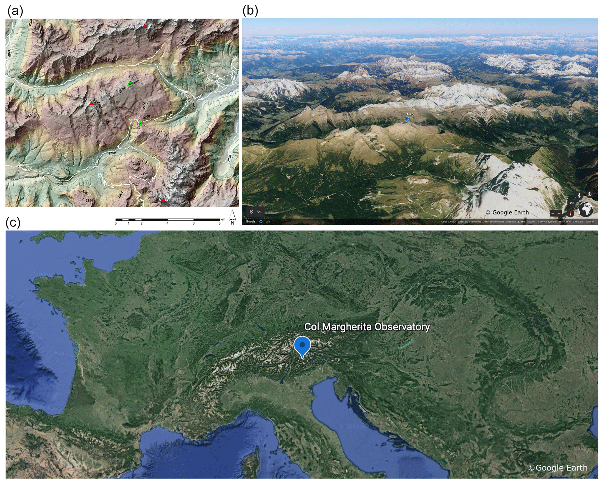
Figure 1 (a) Surrounding area of the Col Margherita Observatory (MRG; 46.36683^∘ N, 11.79192^∘ E; 2543 m a.s.l.). Geographical key points and their distance from the MRG observatory are Passo Valles (SSE) at 2032 m a.s.l. and 3.2 km away, Cima Bocche (ESE) at 2745 m a.s.l. and 3.3 km away, Cima dell'Uomo (NNE) at 3010 m a.s.l. and 4.6 km away and Cimon della Pala (SSE) at 3184 m a.s.l. and 9.3 km away. (b) 3D aerial view of the Col Margherita (© Google Earth). (c) Satellite view of central Europe and the location of the Col Margherita Observatory (© Google Earth).

2.2 MRG observatory description

The MRG observatory is a GAW Regional Station (WIGOS ID 0-380-0-MRG) led by the Institute of Polar Sciences of the National Research Council of Italy (ISP-CNR). It is located on the southeastern side of the Italian Alps (46.36683^∘ N, 11.79192^∘ E), based at an altitude of 2543 m above mean sea level (hereafter m a.s.l.). It was chosen as representative for the surrounding alpine region (Barbaro et al., 2020). The observatory is a prefabricated insulated shelter with external dimensions of 3.00 m × 2.42 m × 3.22 m. The observatory is equipped with a complete automatic weather station mounted on a 3 m mast.

2.3 Low-cost sensors

We used the AlphaSense OX-B431 commercial passive sensor which belongs to the class of electrochemical sensors that operate in amperometric mode. These low-cost sensors are sensitive to ozone (O₃) and nitrogen dioxide (NO₂). These oxidising sensors generate a current that is linearly proportional to the fractional volume of the target gases.

AlphaSense provides a calibration certificate and reference regression coefficients for each sensor. The manufacturer declares that the calibration was conducted in a controlled environment (temperature 22 ± 3 ^∘C; relative humidity 40 ± 15 %) using the ozone generator (Thermo Scientific; model 49i-PS; flow 0.5 L min⁻¹), and it was performed considering two points, i.e. zero and span (1 part per million (hereafter ppm)). The technical sheet (http://www.alphasense.com/, last access: 7 September 2021) reports that the sensor limit of detection is in the range of units of parts per billion (hereafter ppb), a sensitivity that is required for detecting environmental ozone concentration. The manufacturer declares that the sensor voltage output is linear up to 20 ppm of the target gas.

In total, three equivalent sensors were installed on the sensing system in order to evaluate intracompatibility between measurements and calibration stability as a function of time. Laboratory calibration was performed at the Institute of Atmospheric Sciences and Climate (CNR-ISAC) headquarters (Bologna, Italy) before field deployment. Field calibration was evaluated through intercomparison with a reference UV absorption O3 analyser installed at the monitoring site. The reference instrument referred to the standard reference photometer no. 15 (SRP 15) calibration scale (GAW report no. 252; WCC-Empa report no. 19/3) through an intercomparison with the calibrator hosted at the CNR-ISAC laboratory (serial no. 1404860524) in June 2017. The sensing system (Fig. 2) was designed to be easily built. It consists of parts that may be purchased online, and they are easy to replace in case of failure. The sensing system was composed of an International Protection (IP)56 enclosure with three holes for the working low-cost sensors and two additional holes for waterproof power and ethernet connectors. An additional LCS was placed inside the box as a spare sensor. It was not necessary to use it throughout the experiment. The enclosure was neither heated nor regulated nor insulated. Sensor holes, located at the bottom of the enclosure, were watertight with rubber O-ring seals. A bag of silica gel was placed inside the box to keep the environment dry. More detailed description of the hardware components of the sensing system and the approximate cost of the system's part are reported in Sect. S1 in the Supplement.

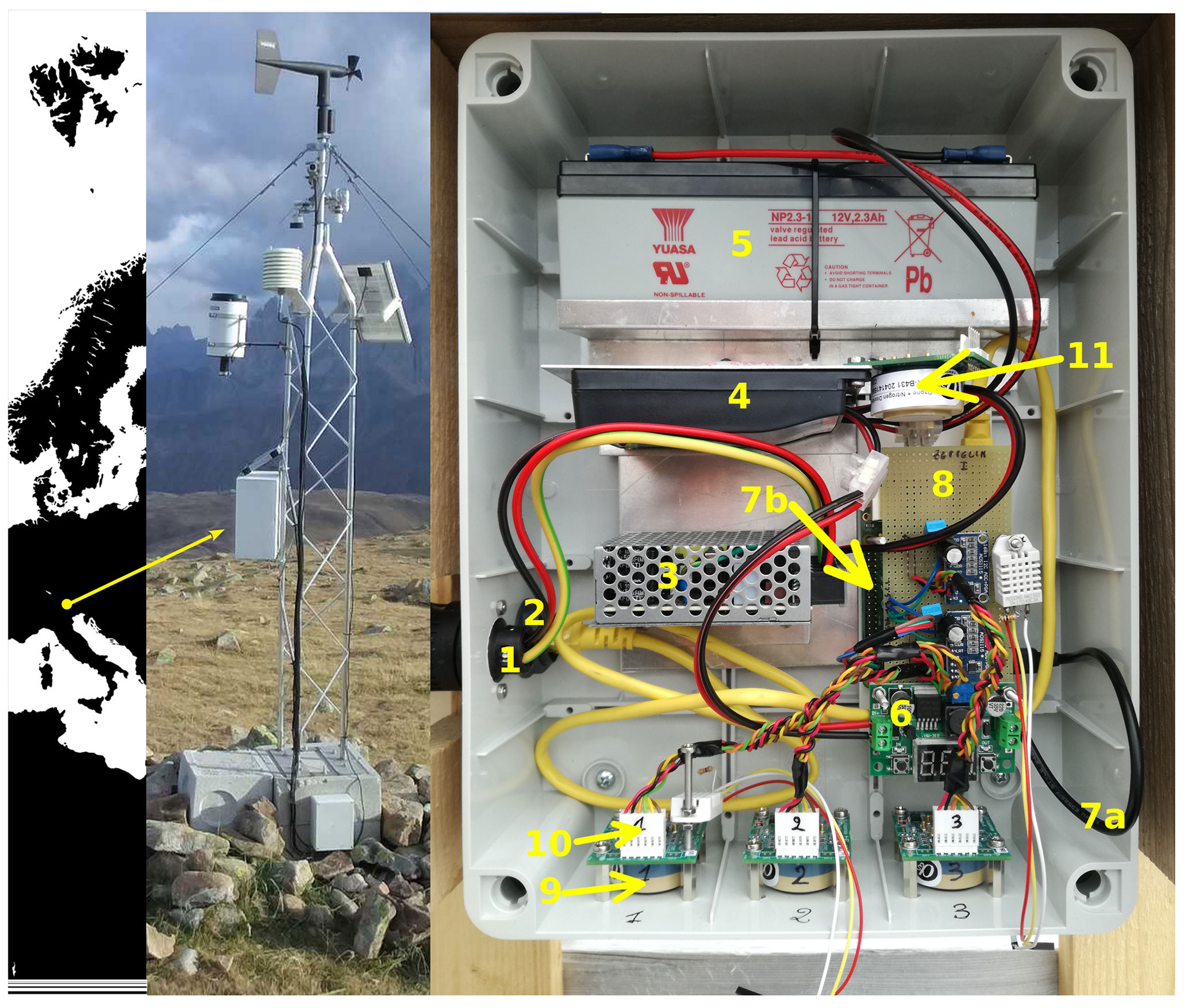
Figure 2 The low-cost sensing system and its components. (1) AC power in, (2) ethernet, (3) power supply, (4) charge regulator, (5) battery, (6) DC/DC converter, (7a) USB power wire, (7b) Raspberry Pi, (8) data acquisition board, (9) working sensor, (10) sensor's plug and (11) spare sensor.

2.4 Sensors calibration

Before field installation, LCSs were calibrated by comparing the analogue voltage output of the low-cost sensors with the ozone concentration generated by an ozone calibrator (Thermo Scientific; 49i-PS) with traceability to the WCC-Empa SRP 15 (calibration in 2017). Each sensor was installed on a specific gassing hood equipped with $\mathrm{1}/{\mathrm{4}}^{\prime \prime }$ (6.35 mm) barbed Swagelok fitting through which the calibration gas was fluxed using a digital mass flow meter. The calibration procedure was designed for the calibration of reference-grade instruments used in the WMO network. It consists of 21 steps in which the reference ozone (flow 0.9 L min⁻¹) spans from 0 to 250 ppb, with a declared precision of 1 ppb and zero noise of 0.25 ppb. Each step lasts for 20 min, and the sensor total calibration time is 7 h. The reference concentration step sequence simulates a pseudo-random variation in ozone concentration. This procedure allows the evaluation of the sensor's tolerance and its ability to respond to sudden and unpredictable (small/large and increasing/decreasing) changes in the ozone concentration, assesses whether the sensor suffers from memory effect or loss of sensitivity and estimates drifts in the instrumental response. The reproducibility and the stability of the sensors calibration parameters were evaluated by performing two laboratory calibrations. In total, three sensors (Mrg1 – AlphaSense serial no. 204141855; Mrg2 – serial no. 204141543; Mrg3 – serial no. 204141544) were calibrated in Bologna between 18 and 19 April 2018, deployed at Col Margherita for a month, then removed on 22 June and re-calibrated between 11 and 12 July under the same conditions of the first calibration. The sensing system was finally re-installed at the Col Margherita Observatory on 17 July. During both calibration periods, the laboratory temperature and humidity were controlled and maintained at ≈ 22.5 ^∘C and ≈ 50 %, respectively. During laboratory calibration, the analogue voltage output of the LCSs was recorded every second. Values were then aggregated to 1 min averages and time matched with the ozone concentration data set generated (1 min) by the reference instrument.

2.5 Field installation and data acquisition parameters

The installation of the sensing system was carried out on 25 May 2018 at the Col Margherita Observatory. The LCS instrument was mounted in the automatic weather station (AWS) mast, 1 m above the ground. The gas inlet through which the reference UV absorption ozone analyser sucks in the air (≈0.6 L min⁻¹) was located on the roof of the observatory at 5 m above the ground. The comparison between the reference instrument in Col Margherita and the LCSs of ozone was performed when both the systems were running, considering the time window from May to December 2018. The analogue voltage output of the LCSs was recorded every 5 s during the field experiment. The values were treated for data processing, as described in Sect. 2.6, then aggregated to hourly averages and finally time matched with the reference ozone concentration data set validated through manual and automatic data preprocessing (Naitza et al., 2020).

2.6 LCS data processing

The LCS raw data were preprocessed to discover possible outliers during the laboratory calibration and the field evaluation. The filter used was based on the computation of a local polynomial (R function LOESS, R Core Team; Cleveland et al., 1992) and the median absolute deviation (MAD) between this polynomial and the measurements within a moving window. We define the outliers as measurements deviating more than 5 times the MAD from the local polynomial (Mueller et al., 2017). If the MAD was smaller than the 50 % quantile of all differences (| local polynomial − measurement |) it was substituted by this value. This approach prevents the exclusion of measurements during time periods with almost no variation on the ozone concentration. We considered a time window of 20 s, chosen after evaluating the time series autocorrelation lag (R function ACF; R core Team; Brockwell et al., 1991) for the laboratory calibration LCS data set. The resulting laboratory calibration outliers were less than the 0.1 % of the total LCS measurements (see Fig. S2.1).

A time window of 1 h was considered before averaging the data to hourly means for the field LCS data set. This procedure excluded less than 0.5 % of 5 s raw data, mainly generated during the turning on phase of the LCS system (see Fig. S2.2). Minutes containing fewer than nine valid observations (75 %) were excluded, and hourly averages were considered if there were data for at least 45 min (75 %). Besides, 82 h for the Mrg2 sensor were manually excluded from the data set. From 01:00 Central European Time (CET) on 5 November to 23:00 CET on 8 November, the WE electrode of the Mrg2 sensor showed completely different behaviour compared to the other two sensors (see Fig. S2.3).

Harsh weather conditions caused many periods of absence of the main AC current at MRG observatory. This made the reference ozone data set discontinuous during the summer. On 14 September, a problem in the pump of the reference instrument was diagnosed, and the reference instrument was dismantled for maintenance until the 25 October. On 29 October, we faced a power outage due to a severe storm (Storm Adrian; see Fig. S5.1). Another problem with the pump of the reference instrument was encountered on 14 December, and the instrument was dismantled.

Therefore, the final comparison between the reference instrument and the LCSs of ozone was performed on the ≈ 45 % of the LCS data, considering the time window from 30 May to 14 December 2018, when both the systems were running.

Evaluation of LCS accuracy was considered by skimming the data to see if the threshold value for relative humidity (RH) had been overcome. We considered a multivariate analysis of variance (ANOVA) model to evaluate the effect of the meteorological variables on the LCS measurements.

The limit of detection (LOD) was calculated as the average zero signal plus 3 times the standard deviation. The limit of quantitation (LOQ) was calculated as the average zero signal plus 10 times the standard deviation (Analytical Methods Committee, 1987; Standardization, 2019; Harris, 2010).

3 Results

3.1 Laboratory calibration of LCSs

Laboratory calibration was performed through a linear model as follows:

$$\begin{array}{}\text{(1)}& V_{\mathrm{OUT}}={\mathit{\beta }}_{\mathrm{0}}+{\mathit{\beta }}_{\mathrm{1}}\cdot \left[O_{\mathrm{3}}\right],\end{array}$$

where $V_{\mathrm{OUT}}=V_{\mathrm{WE}}-V_{\mathrm{AUX}}$ is the LCS analogue output signal, [O₃] is the ozone reference concentration in parts per billion (ppb), β₀ (millivolt; hereafter mV) is the intercept, and β₁ (millivolts per parts per billion; hereafter mV ppb⁻¹) is the slope. Linear model agreement between the reference and the LCS was evaluated using the Pearson correlation coefficient (PCC). Evaluation of bias was performed using the mean absolute error (MAE) as follows:

$$\begin{array}{}\text{(2)}& \mathrm{MAE}={\displaystyle \frac{{\sum }_{i=\mathrm{1}}^n\left|e_i\right|}{n}},\end{array}$$

where e_i was the difference between the prediction (y_i) and the true value (x_i, $e_i=y_i-x_i$), and n was the number of observations.

A summary of the calibration experiments and comparison with the calibration values declared by AlphaSense is reported in Table 1. As an example of the laboratory experiment, the Mrg1-calibrated ozone measurements and analogue output signal registered against the reference ozone in July are shown in Fig. 3, using the main and secondary y axis, respectively. The linear regressions of the laboratory calibrations are shown in Fig. 4. We did not see a change in the analytical performances of the LCSs between the two calibration experiments (two sample t test; p value >0.7). The mean voltage response of Mrg1 was 18.1 ± 0.6 mV, when reference ozone concentration was 0.4 ± 0.1 ppb, and reached 100.2 ± 0.6 mV, when reference ozone concentration was 249.75 ± 0.04 ppb. The precision of the Mrg1 sensor, calculated as the relative standard deviation (RSD), was ≈ 3.2 % close to the LOD and decreased to ≈ 0.6 % for ozone concentrations higher than 200 ppb (Thompson, 1988; Horwitz and Albert, 1997; see Fig. S4.1). MAE for Mrg1 was 3.6 ppb, LOD for Mrg1 was 4 ppb and LOQ for Mrg1 was 14 ppb. The instrumental response to the ozone concentration was linear in the interval considered (R²=0.998). Through our laboratory experiment, we can confirm the linear dynamic range (LDR) for Mrg1 between the LOD (4 ppb) and 250 ppb. The AlphaSense data sheet reports that the instrumental response of the OX-B431 sensor was linear up to 2 ppm. Details on results for Mrg2 and Mrg3 can be found in Sect. S4.

Compared to the linear regression parameters given by the manufacturer, we obtained an average difference of about 4.2 % on the intercept and an average difference of about 21.6 % on the slope.

Table 1 In the first half of the table, the linear model regression coefficients and accuracy metrics obtained during the laboratory calibration are reported. Pearson correlation coefficient (PCC), intercept (β₀), regression coefficient (β₁), linear dynamic range (LDR), relative standard deviation limits (RSD), bias (MAE), limit of detection (LOD) and limit of quantification (LOQ) are shown. In the second half of the table, below the regression coefficients, intercept (${\mathit{\beta }}_{\mathrm{0}}^{\prime }$) and slope (${\mathit{\beta }}_{\mathrm{1}}^{\prime }$) transcribed from sensor's data sheet are reported. Mean absolute error (MAE) between ${\mathit{\beta }}_i^{\prime }$ and β_i (averages) is given in the first two columns. LCS statistics have been performed over 300 1 s values for each ozone concentration step for a total of ≈ 6.5 k calibration points per sensor. Significant digits are in accordance with the calibration data sheet.

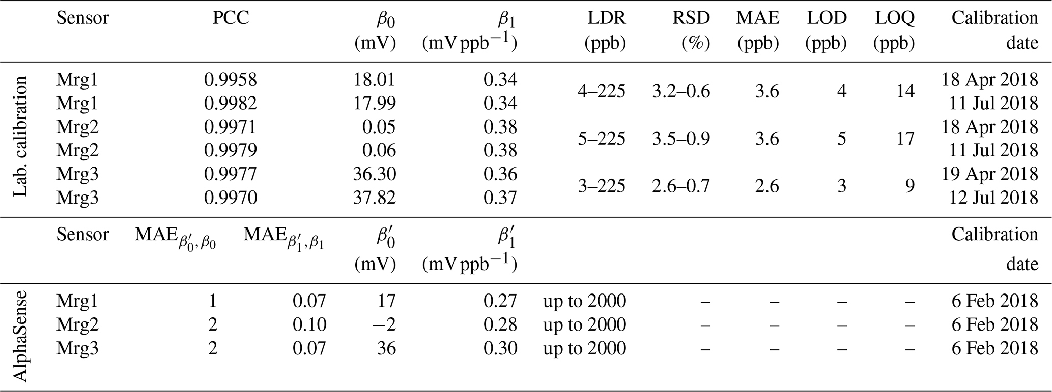
Figure 3 After calibration, voltage data (V_OUT) of the low-cost sensor is expressed in ppb (black) and compared to the reference ozone concentration (green). The sensor's ozone concentration, obtained using the intercept, and the regression coefficient, provided by AlphaSense, are also shown (grey). Calibration date is 11 July 2018.

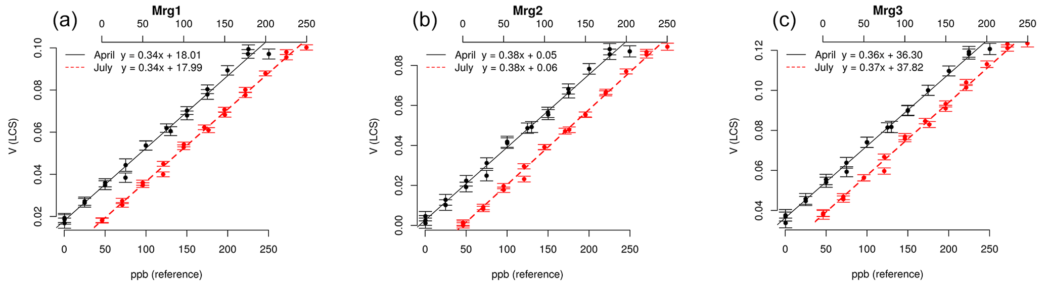
Figure 4 Laboratory calibration of the low-cost sensors. Linear regressions obtained during April (black) and July (red) are shown. From left to right, the results for sensors Mrg1, Mrg2 and Mrg3 are reported, respectively. To improve the visibility of the graphs, two shifted x axes are given. The bottom axis refers to the April experiment, while the upper axis refers to the July experiment.

3.2 Field experiment

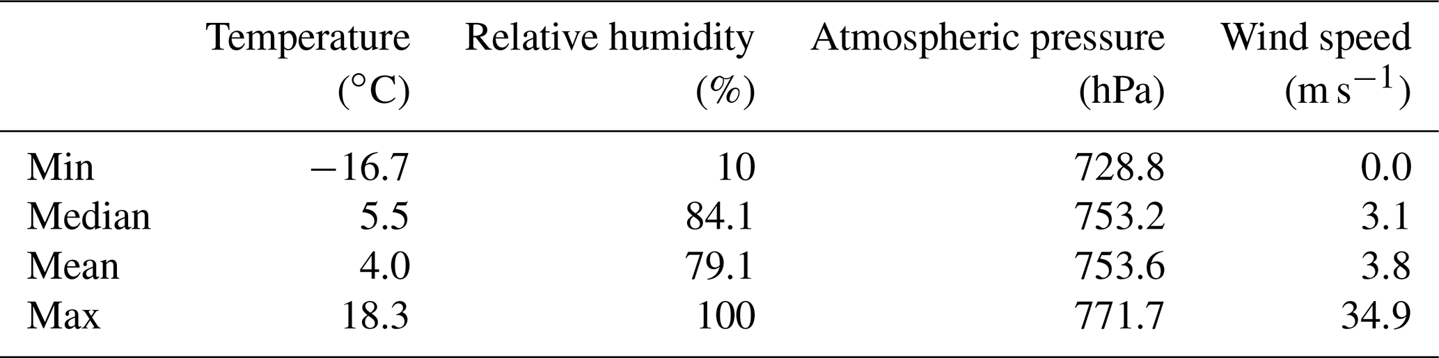
Field measurements were conducted from 30 May to 14 December 2018. We measured about 4800 h data that were collected in a wide range of environmental temperatures (degrees Celsius), pressures (hectopascals), wind speeds (metres per second) and RH (percent), as summarised in Table 2.

Table 2 Summary of the meteorological data (temperature, relative humidity, atmospheric pressure and wind speed) recorded at Col Margherita during the field experiment from 30 May to 14 December 2018.

3.3 Correlation and bias between LCSs – intracomparison

A first estimate to verify that the LCSs were in agreement with each other during field measuring was done calculating their PCC and bias, referred to as MAE, throughout the period considered and their variation trends over time. A summary of the inter-PCC and inter-MAE trends is reported in Table 3. The comparison is consistent, except for the month of October. Out of the 744 h observations collected during the month, only 59 observations were considered for the analysis, which is when both the LCS system and the reference instrument were working (from 25 to 28 October; see Sect. 2.6). Since there were no signs of malfunction, and given the low environmental variability in the ozone concentration during the 3 d analysed (29 ppb < O₃ < 47 ppb calculated by the reference instrument and 25 ppb < O₃ < 46 ppb calculated averaging the LCS measurements), we hypothesised that the low correlation value between LCSs could have been due to the inherent variability in the sensors' measurements. Indeed, if all 744 LCS hourly observations in October were considered, we could have calculated the following: PCC${}_{\mathrm{1},\mathrm{2}}=\mathrm{0.86}$, PCC${}_{\mathrm{1},\mathrm{3}}=\mathrm{0.85}$ and PCC${}_{\mathrm{2},\mathrm{3}}=\mathrm{0.86}$, which is a result consistent with the other periods described in Table 3.

The statistical analysis over 1772 h observations from 30 May to 14 December gives ${\mathrm{PCC}}_{\mathrm{1},\mathrm{2}}=\mathrm{0.90}$, PCC${}_{\mathrm{1},\mathrm{3}}=\mathrm{0.95}$ and PCC${}_{\mathrm{2},\mathrm{3}}=\mathrm{0.93}$, while MAE${}_{\mathrm{1},\mathrm{2}}=\mathrm{4.4}$ ppb, MAE${}_{\mathrm{1},\mathrm{3}}=\mathrm{2.8}$ ppb and MAE${}_{\mathrm{2},\mathrm{3}}=\mathrm{4.4}$ ppb.

Table 3 Stability of LCS intracorrelation (PCC_i,j) and bias (MAE_i,j), considering the period from 30 May to 14 December 2018. The indices i and j refer to the LCSs between which the comparison is made, e.g. PCC_1,2 is the Pearson correlation between the sensors Mrg1 and Mrg2. For each statistical metric, its total, monthly values and the number of hourly observations that are used to perform the calculation are reported.

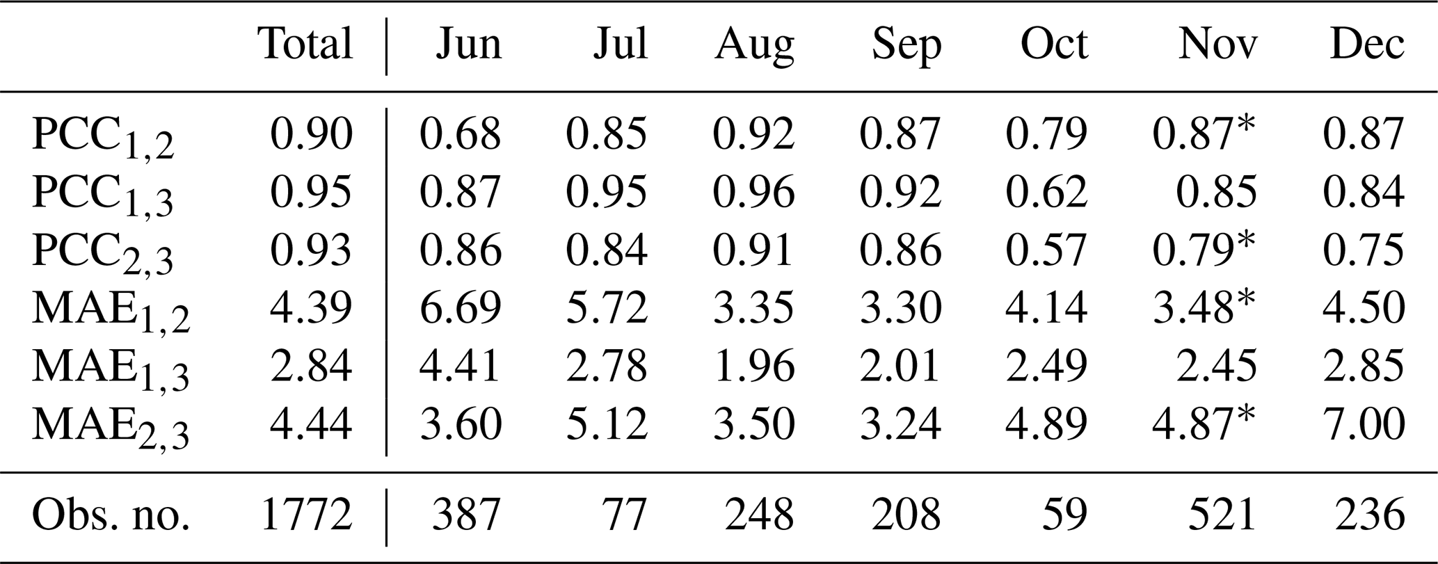
^* Due to the malfunction of the Mrg2 sensor, 82 h observations from 5 to 8 November 2020 of this sensor have been excluded from the LCS data set.

3.4 Correlation and bias between low-cost sensors and reference – intercomparison

We measured the correlation and the bias between the LCSs and the reference instrument to evaluate the performances of the LCSs in a real-case scenario where there could be no possibility to improve the laboratory calibration model. In addition to the calculation of the MAE, we consider also the root mean square error (RMSE) and, to highlight the sign of the bias, the mean bias error (MBE), defined as follows:

$$\begin{array}{}\text{(3)}& {\displaystyle }& {\displaystyle }\mathrm{RMSE}=\sqrt{{\displaystyle \frac{{\sum }_{i=\mathrm{1}}^n(e_i{)}^{\mathrm{2}}}{n}}}\text{(4)}& {\displaystyle }& {\displaystyle }\mathrm{MBE}={\displaystyle \frac{{\sum }_{i=\mathrm{1}}^n{e}_i}{n}}.\end{array}$$

In this context, the true value is the ozone measured by the reference instrument in Col Margherita. The statistical analysis, considering both the whole data set and the trend of each sensor, is reported in Table 4. On average, the PCC between the sensors and the reference was ≈0.8, with the smallest values registered in December. The average MAE was ≈5 ppb, and RMSE was ≈7 ppb. The bias was not constant through the period. It was larger during summer, and it decreased during autumn, with the MBE showing a change in the sign. Probable causes that might affect the accuracy of the LCS measurements could be the environmental temperature and relative humidity, whose dependence is also described in the sensor data sheet and further investigated in Sects. 3.4.1 and 3.5.

We observed cases with poor agreement. Perhaps lower ozone concentrations and/or low environmental variation in ozone concentrations encountered in the midwinter periods influenced the data quality from the sensors or even the reference instrument. This could explain the low correlation observed during December. Also, as discussed in Sect. 3.3, we hypothesised that the low correlation value between LCSs and reference during October could have been due to the short amount of time where both systems were running. The cases of June for Mrg2 and all the LCSs during July were peculiar. Perhaps a role played by the temperature difference between the inside and outside of the box could explain the lower correlation.

Table 4 Intercorrelation and bias between the LCSs calibrated in the laboratory and the reference. Statistical metrics considered are the Pearson correlation coefficient (PCC), mean absolute error (MAE), root mean square error (RMSE) and mean bias error (MBE). For each statistical metric, its total, monthly values and the number of hourly observations that are used to perform the calculation are reported. The sum of the hourly observations in the monthly analysis differs from the total of 1793 observations by the data from 31 May to 14 June.

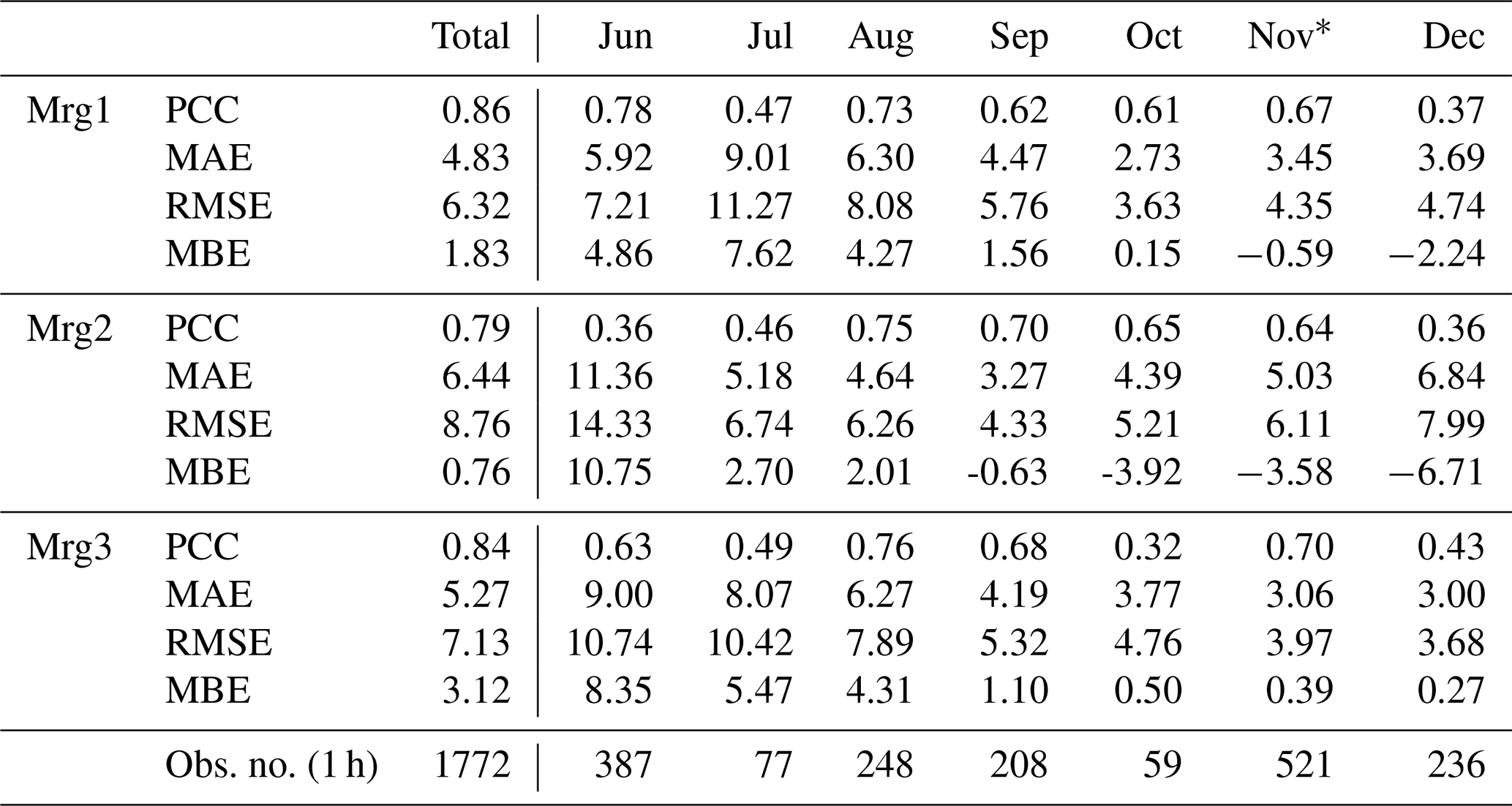
^* Due to the malfunction of the Mrg2 sensor, 82 h observations from 5 to 8 November 2020 of this sensor have been excluded from the LCS data set.

3.4.1 Relative humidity threshold

The AlphaSense Application Note 106 (AAN 106) reports that the low-cost sensors must operate in a RH range from 15 % to 90 %. We evaluated that the exclusion of the observations collected outside the RH interval does not improve the correlation and accuracy metrics between the LCSs and the reference instrument. Thus, considering the poor improvement obtained through skimming, we did not exclude further LCS measurements from the data set.

3.5 Environmental low-cost sensors model

We evaluated the relationship between the bias and the temperature, relative humidity, atmospheric pressure, solar radiation, wind speed and wind direction to further investigate which meteorological variables were contributing to the bias (e_i) between the LCSs (${\mathrm{O}}_{\mathrm{3}}^{\mathrm{lcs}}$) and the reference ozone concentration (${{\mathrm{O}}_{\mathrm{3}}}^{\mathrm{R}}$). Figure 5 shows the correlation plots for temperature, relative humidity and LCS signal, while the remaining plots for the non-correlating variables are reported in Fig. S5.6. The bias showed a correlation trend with the air temperature (PCC ≈0.53; p value $<\mathrm{2}e-\mathrm{16}$) and relative humidity (PCC ≈0.45; p value $<\mathrm{2}e-\mathrm{16}$), while no evidence of correlation was shown with the incident solar radiation (PCC ≈0.05; p value ≈0.1), the atmospheric pressure (PCC ≈0.24; p value ≈0.3), the wind speed (PCC $\approx -\mathrm{0.22}$; p value ≈0.1) or the wind direction (PCC $\approx -\mathrm{0.10}$; p value ≈0.4). We finally observed that the bias was dependent on the sensor signal itself (PCC ≈0.55; p value $<\mathrm{2}e-\mathrm{16}$).

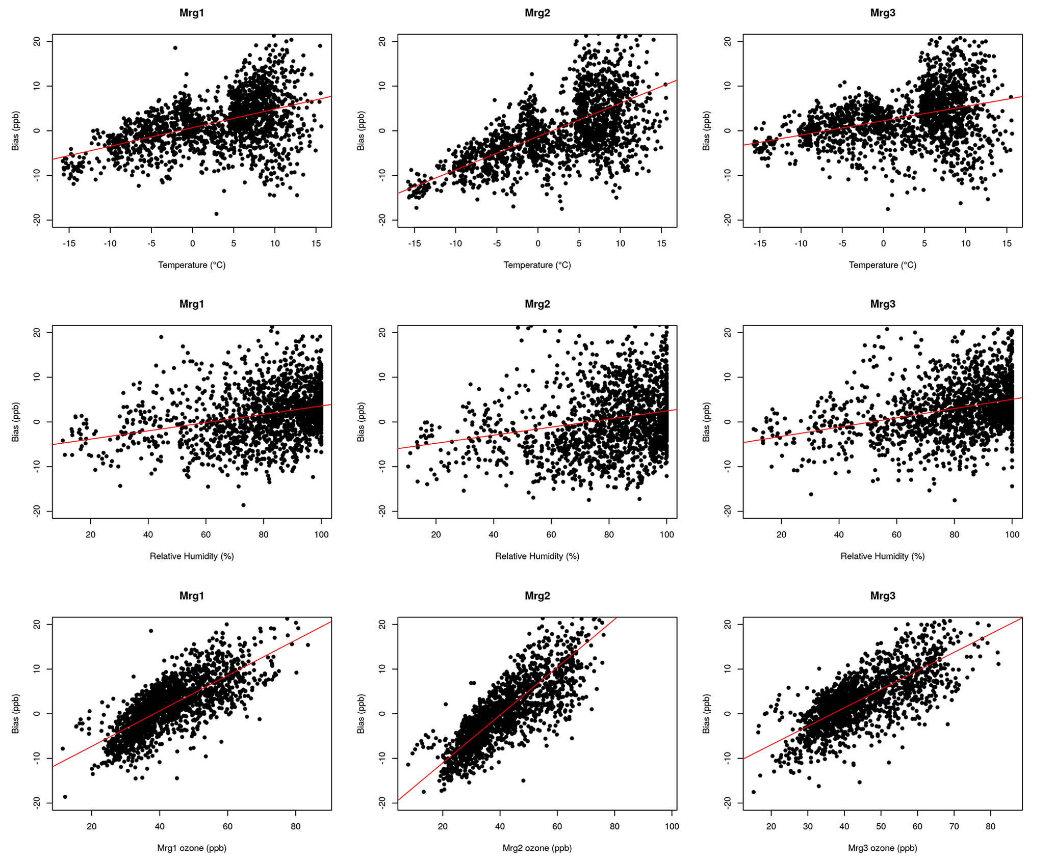
Figure 5 The environmental variables with a non-negligible linear correlation with the LCS bias.

We considered the following statistical multivariate linear model to evaluate the sensors bias under specific meteorological conditions and LCS signal, implementing in the model only the explanatory variables as previously described:

$$\begin{array}{}\text{(5)}& e_j=a_{\mathrm{0},j}+a_{\mathrm{1},j}T+a_{\mathrm{2},j}\mathrm{RH}+a_{\mathrm{3},j}{{\mathrm{O}}_{\mathrm{3}}}^{\mathrm{lcs},j},\end{array}$$

where bias (e_j, $j=\mathrm{1},\mathrm{2},\mathrm{3}$) is the difference in the ozone concentration measurement between the jth LCS and the reference, a_i,j denote the model coefficients, T is the ambient air temperature, RH is the relative humidity, and ${{\mathrm{O}}_{\mathrm{3}}}^{\mathrm{lcs},j}$ are the jth LCS ozone readings obtained from Eq. (1).

We thus used Eq. (5) to improve the laboratory calibration model and to achieve a better estimation of the field (F) ozone concentration measured by the jth low-cost sensors (${{\mathrm{O}}_{\mathrm{3}}}^{F,j}$) as follows:

$$\begin{array}{}\text{(6)}& {{\mathrm{O}}_{\mathrm{3}}}^{F,j}={{\mathrm{O}}_{\mathrm{3}}}^{\mathrm{lcs},j}-e_j.\end{array}$$

3.6 Performance of the model

We considered three case scenarios to evaluate the performance of the model. A summary of the values obtained are reported in Table 5.

3.6.1 Scenario 1

The first scenario considered the whole reference data set to model the bias and correct the LCS measurements. The intercorrelation between the LCSs and the reference improved by ≈1 %. The accuracy between the LCS measurements and the reference improved by ≈60 %, lowering the average bias (MAE) from ≈5.5 to ≈3.2 ppb, with 50 % of the bias distribution between $\approx \pm \mathrm{2.5}$ ppb and 95 % between $\approx \pm \mathrm{8.5}$ ppb (Fig. 6). The corrected LCS data set, obtained by the continuous calibration of the LCSs in Col Margherita, could be used to reconstruct the environmental ozone concentration in case of loss of reference data, a situation that may occur due to power outages or during the instrumental calibration when the reference instrument is not present at the observatory. During our experiment, we obtained 1556 1 h additional ozone measurements, considering the time periods where the LCSs and the AWS were collecting data (see Sect. S5).

Figure 6 (a) Bias between the reference instrument and the Mrg1 sensor after the LCS correction, (b) bias of the Mrg2 sensor after LCS correction, (c) bias of the Mrg3 sensor after correction and (d) comparison of the LCS bias before and after correction.

3.6.2 Scenario 2

A second scenario still considered the whole reference data set, but it aims to evaluate the intracompatibility of the LCS bias model. This might be useful if considering the use of the bias model of one low-cost sensor for the calibration of another low-cost sensor. This approach opens the possibility of performing a remote calibration in the surrounding area of the Col Margherita. A remote calibration allows the deployment of a local sensor network where the remote stand-alone sensor's signal is corrected using the bias model studied in a location where a reference instrument is always present. We compared the coefficients of the bias model of each low-cost sensor. Subsequently, we evaluated the accuracy between one of the LCSs and the reference, correcting its data set using the averaged model coefficients of all the three LCSs (scenario 2a). Next, we evaluated the accuracy between a LCS and the reference, correcting its LCS data set using the averaged value of the other two LCS coefficients (scenario 2b). The average value of the intercept coefficient (a₀) is −27.76 ± 8.94 %. The average value of the temperature coefficient (a₁) is 0.26 ± 8.11 %. The average value of the RH coefficient (a₂) is 0.11 ± 5.41 %, and the average values of the LCS coefficient (a₃) is 0.45 ± 11.32 %.

3.6.3 Scenario 2a

We considered the average coefficient values and their relative standard deviations to model the bias of each sensor and to calculate the corrected LCS ozone data set. In this scenario the intercorrelation between the LCSs and the reference improved by ≈1 %. The accuracy between the LCS measurements and the reference improved, lowering the average bias (MAE) to ≈3.3 ppb. In total, 50 % of the bias distribution confidence interval (CI) was $\approx \pm \mathrm{2.6}$ ppb, and the 95 % CI was $\approx \pm \mathrm{8.7}$ ppb.

3.6.4 Scenario 2b

We corrected the ozone measurements of each low-cost sensor using the average model coefficients of the other two low-cost sensors. The intercorrelation metrics between the LCSs and the reference improved by ≈1 %. The accuracy between the LCS measurements and the reference improved, lowering the average bias (MAE) to ≈3.5 ppb. In total, 50 % of the bias distribution CI was $\approx \pm \mathrm{3}$ ppb, and the 95 % CI was $\approx \pm \mathrm{9}$ ppb.

3.6.5 Scenario 3

The third scenario examined the execution of consequential field calibrations. It represents the situation where there is no chance to lay on local or remote calibration. The low-cost sensing system has to be installed alone, except for scheduled calibration periods during which a reference instrument is placed aside the low-cost sensor to model the bias. The calibrating periods must be chosen to depict as much as possible all the seasonal meteorological conditions of the site.

We modelled the bias considering only the June and the December reference data set. These periods represent the annual extremes of the meteorological conditions at Col Margherita (Table 2 and Sect. S5.2). Data used for field calibration are 423 1 h observations from 30 May to 21 June 2018 and 236 1 h observations from 1 to 14 December 2018.

In this scenario, the intercorrelation between the LCSs and the reference improved by ≈1 %. The accuracy between the LCS measurements and the reference improved by lowering the average bias (MAE) to ≈3.3 ppb. In total, 50 % of the bias distribution CI was $\approx \pm \mathrm{2.7}$ ppb, and the 95 % CI was $\approx \pm \mathrm{8.7}$.

Table 5 Summary of the performances of the LCS bias model in the three scenarios considered. In scenario 1, we corrected one LCS bias using its environmental model coefficients within the full data set. In scenario 2a, we corrected a LCS bias averaging the environmental model coefficients of all the LCSs within the full data set. In scenario 2b, we corrected a LCS bias averaging the environmental model coefficients of the others two LCSs within the full data set. In scenario 3, we corrected a LCS bias using the LCS calculated environmental model coefficients considering only the annual extremes meteorological conditions at Col Margherita. For each case, the final Pearson correlation coefficient (PCC) and mean absolute error (MAE) between the low-cost sensor and the reference instrument, the bias distribution median and the bias distribution confidence interval (CI) at 95 % are reported.

4 Discussion

We summarised the LCS analytical performance results obtained through two laboratory calibration experiments and a ≈7 months field experiment performed at the Col Margherita Observatory.

4.1 Detection limits

The LCSs were capable of detecting ozone in the typical environmental ppb range. During the laboratory calibration experiments, we observed that the LOD of the LCSs was about 5 ppb, and the LOQ was about 15 ppb. We noticed that the LCS response to ozone concentration was linear (PCC >0.99) up to 250 ppb, and these analytical performances of the LCSs did not change after two laboratory calibration experiments conducted 3 months apart from one another. When used in the field, the linear regression coefficients obtained through laboratory calibration, at fixed temperature and humidity, are not capable of fully describing the behaviour of the LCSs (PCC ≈0.8).

4.2 LCS calibration

We observed that all the sensors require an individual double calibration (both in laboratory and in the field), and that the calibration values declared by the manufacturer could be insufficiently accurate for an environmental study. Attention should be paid when deciding whether to perform a single field calibration (few days), since this can be insufficient; it is very unlikely that one single calibration exercise is representative of the environmental and meteorological conditions of a whole year. A solution, which increases the logistic efforts and costs, might be to perform many field calibrations covering at least the extremes of the meteorological year condition, in order to depict as much as possible the behaviour of the sensors in the environment. An attractive solution might be to perform a remote calibration. We showed that we can improve the LCS accuracy using the bias correction coefficients optimised for other similar LCSs (scenario 2b). Our results represent an “optimum level” of performances since we used the entire data set to derive the calibration coefficients, and the performance of the remote calibrations was evaluated under very similar meteorological and environmental conditions. Given these fascinating results, further studies on the accuracy and robustness of a remote calibration will be conducted.

4.3 Precision

The evaluation of the LCS intracorrelation during the field experiment revealed that the sensors behave in a similar but not identical way (intra-PCC≈0.9); thus, it is important to increase the reliability and reproducibility of the measurements considering LCS redundancy. This is particularly important when using the sensors in the field without any reference. We indeed detected a case during which one of the three LCSs was not working properly (Fig. S2.3). These anomalies could not be detectable if redundancy is not considered. The precision of the LCSs, described by the RSD, was evaluated in the laboratory with a constant reference ozone concentration. We observed that, near the LOD, the LCS RSD is ≈3.5 %, decreasing to ≈1.6 % at ≈50 ppb, and reaches the asymptotic value of ≈0.8 % for larger ozone concentrations (>200 ppb). We did not notice a deterioration of the LCS precision between the two laboratory calibration experiments. During the field campaign it is not trivial to evaluate the precision in terms of RSD because there is neither a constant reference ozone concentration nor a constant meteorological situation. Thus, since it is not possible to evaluate the precision in field, we assumed that the precision during the field experiments was compatible with the precision studied in the laboratory.

4.4 Bias

The LCS average bias, measured through the MAE between the LCS and the reference instrument during the field experiment, was ≈3.5 ppb (≈ 6 ppb without performing the bias correction). The LCS electrical noise measured in the laboratory was ≈1.5 ppb (see Fig. S3.1) and bias >4 ppb. During the field experiment, we observed that the LCS bias is dependent on the air temperature, RH and the LCS electrodes voltage. It is possible to build a multivariate linear model able to describe about 60 % the bias variance during the period in which the LCS operates in co-location with the reference instrument. It is of interest that the environmental model coefficients do not differ much from one another (≈ 8.5 %). We noticed that it is possible to reduce the bias of one LCS using the average coefficient values of another LCS, suggesting the possibility of performing a remote field calibration of the sensors in the surrounding area of the observatory.

4.5 Reliability

We have not measured differences in the analytical performances between the two LCS calibration experiments. We showed that, during the field experiment, the LCS response to the reference ozone concentration was affected by the local meteorology, and its dependence can be analytically described. We observed that a time-dependent model for correcting the bias was not necessary for our field experiment but would be reasonably needed for long-term monitoring when LCS ageing will not be negligible. The rapid response (≈30 ppb s⁻¹) and the small memory effect, measured both during the laboratory experiments and in the field experiment, allowed the measurement of rapid variations in the ozone concentration.

The sensor's data sheet reports that NO₂ interferes with the ozone measurements. Since there was not a NO₂ analyser during our field experiment at the MRG observatory, we were not able to measure the concentration of this gaseous pollutant. We referred to a local study (Costantino, 2016) to deduce the amount of NO₂ that could have interfered with our experiment. This work was based on the data of the regional environmental agency and included a survey on ozone and nitrogen dioxide at Passo Valles (2.032 m a.s.l., about 3.2 km away from the MRG and about 500 m lower in altitude than MRG) was conducted from 1 January 2007 to 1 January 2011. The average annual concentration of NO₂ at Passo Valles was 2±1 ppb, and the average annual concentration of ozone was $\approx \mathrm{47}\pm \mathrm{3}$ ppb. As a comparison, despite referring to different years, the ozone concentration at Col Margherita was $\approx \mathrm{40}\pm \mathrm{10}$ ppb during 2018, ≈15 % lower than what was recorded at Passo Valles. It is worth noticing that the monitoring site at Passo Valles is next to a road, which could be a local source of NO₂ pollution. Therefore, even if it was not possible to know the NO₂ concentration at MRG, the mean values measured at Passo Valles suggest that a few ppb of NO₂ may have interfered with our experiment at MRG. Nevertheless, it has been observed that NO₂ concentrations are decreasing all over Europe (Jamali et al., 2020; Castellanos and Boersma, 2012), with mean average values ranging from 0.15 to 0.36 ppb, while the 25th and 50th percentiles ranged from 0.05 to 0.19 ppb and from 0.16 to 0.40 ppb, respectively (Cristofanelli et al., 2021). It is unlikely that NO₂ interference could have been detected by our LCS system in MRG and, thus, explains some of the bias we observed between the LCSs and the reference instrument.

We showed that the LCSs was subjected to many considerable “stresses” throughout the field experiment. During the summer period, we faced some severe power outages which caused data losses. These events were due to heavy thunderstorms and bad weather conditions that are characteristic of the alpine summer season. Moreover, the LCSs faced a severe storm (Storm Adrian on 29 October 2018; see Fig. S5.1) which caused a great deal of damage all through the north of Italy and caused a general blackout in the Col Margherita area. It is worth noting that the LCS system was the only one that remained on during the Storm Adrian storm blackout. When the power returned, the system showed no damage.

5 Conclusions

We found that O₃ low-cost gas sensors can provide concentration measurements with a bias of only a few ppb (±8.5 ppb at 95 % of confidence) throughout the period of field operation. We found that all of the sensors required an individual calibration. We observed that laboratory calibration is not sufficient to explain the behaviour of the sensors during this field experiment. Therefore, performing a sensor field calibration near a reference site is necessary, and this requires infrastructure. Since the quality of the sensor calibration depends on the description of the environmental conditions (i.e. pollutant concentrations and meteorology), we showed that reference instrumentation is necessary for performing periodic field calibrations. In this work, we discussed three procedures for field calibration of the LCSs. We showed how to improve the LCS analytical performance when a reference instrument is always present or when it is available for scheduled calibration periods. Finally, we showed how to improve O₃ measurements of stand-alone LCSs with a remote calibration prototype. Comparison with a reference-grade instrument revealed that the sensor's bias is impacted by changes in environmental temperature and relative humidity. These effects can be reduced by applying a correction function, and we showed that a multivariate linear model can describe up to 60 % of the bias variability. We noticed that the bias model coefficients were comparable between each sensor (≈8.5 % of difference). Demonstrating the possibility of performing remote calibrations of low-cost sensors without a reference instrument. Future studies should focus on the improvement of the mathematical description of the LCS working principle, and on their environmental dependence, to evaluate to what extent a single bias model could be used for a sensors network in an alpine area. Achievable technical improvements for the enhancement of the analytical performance of the LCS system are still open as low-cost technology improves. Other improvements include an improved housing for the sensing system with thermal insulation and humidity control, while ensuring circulation of ambient air that does not impact the energy efficiency of the instrument. This study demonstrates how to obtain valuable ozone data from a low-cost instrument in a remote, harsh, high-altitude alpine environment and shows procedures for the design of adequate monitoring strategies in the study of tropospheric gases in remote areas.