the Creative Commons Attribution 4.0 License.
the Creative Commons Attribution 4.0 License.
 | 16 Sep 2021
Application of a mobile laboratory using a selected-ion flow-tube mass spectrometer (SIFT-MS) for characterisation of volatile organic compounds and atmospheric trace gases
Rebecca L. Wagner
Naomi J. Farren
Jack Davison
Stuart Young
James R. Hopkins
Alastair C. Lewis
David C. Carslaw
Over the last 2 decades, the importance of emissions source types of atmospheric pollutants in urban areas has undergone significant change. In particular, there has been a considerable reduction in emissions associated with road vehicles. Understanding the role played by different source sectors is important if effective air pollution control is to be achieved. Current atmospheric measurements are made at fixed monitoring sites, most of which do not include the measurement of volatile organic compounds (VOCs), so our understanding of the temporal and spatial variation of pollutants is limited. Here we describe the application of a mobile laboratory using a selected-ion flow-tube mass spectrometer (SIFT-MS) and other trace gas instrumentation to provide on-road, high-spatial- and temporal-resolution measurements of CO2, CH4, VOCs and other trace gases. We then illustrate the potential of this platform for developing source characterisation methods that account for the similarity in correlation between species. Finally, we consider the benefits of high-spatial- and temporal-resolution measurements in characterising different types of sources, which would be difficult or impossible for single-species studies.
- Article
(10828 KB) - Full-text XML
- BibTeX
- EndNote


Air pollution in many urban areas is a major problem due to a myriad of emissions sources and dense populations, leading to increased potential for human exposure. Among important air pollutants, volatile organic compounds (VOCs) are a class of pollutants that can significantly affect the chemistry of the atmosphere and human health. VOCs play an important role in atmospheric chemistry as they react rapidly with hydroxyl radicals and nitrogen oxides in the presence of sunlight to form products such as ozone (O3) (Zhang et al., 2019) and peroxyacetyl nitrate (Roberts, 1990; Roberts et al., 2003). O3 can cause respiratory irritation (Nuvolone et al., 2018) and damage to ecosystems (Grulke and Heath, 2020). Peroxyacetyl nitrate has been shown to have adverse effects on plant growth and human health at high concentrations (Vyskocil et al., 1998), and it has also been shown to thermally decompose to form NOx, which leads to enhanced O3 production (Heald et al., 2003). VOCs themselves can undergo gas-to-particle conversions to produce secondary organic aerosol (Kourtchev et al., 2016). Also, some VOCs can cause acute irritations and damage to internal organs (Shuai et al., 2018), and chronic human exposure to benzene can induce haematological problems and cancer (Kampa and Castanas, 2008).
To combat air quality and health issues in urban areas, it is important that the composition and sources of VOCs are understood. Vehicular emissions of VOCs have historically been of central importance to issues such as O3 and secondary organic aerosol formation. But the composition and sources of these species in urban areas are highly complex, and it is difficult to determine the role played by VOCs from road vehicles relative to other sources. While VOC emissions from vehicle exhaust have been aggressively reduced over the past few decades in Europe through the introduction of technologies such as three-way catalysts on gasoline vehicles, they still present an important source of emissions, accounting for 4 % of total UK VOC emissions in 2017 (Lewis et al., 2020).
Nevertheless, the reduction in vehicular emissions means it is likely that other sources of emissions, such as volatile chemical products (VCPs), solvent use, cooking, residential wood burning and industry, have become more important. Mass balance analysis by McDonald et al. (2018) concluded that emissions from VCPs now account for half of the fossil fuel VOC emissions in industrialised cities. Lewis et al. (2020) estimated that in the UK, VOC emissions from solvent use and industrial processes account for 63 % of total VOC emissions. This change in the contribution of VOC emissions from different sources is not reflected in current VOC measurements made at stationary monitoring sites in the UK, which measure only 13 of the 20 most significant VOCs (Lewis et al., 2020) due to set-up taking place 30 years ago when road transport was the dominant VOC emissions source.
The current understanding of urban air pollution depends on hourly or daily measurements of a limited number of atmospheric pollutants recorded at stationary monitoring sites. These measurements are unable to represent relative contributions of different source types and complex temporal and spatial variations of pollutants. To overcome this problem, mobile laboratories equipped with fast-response instruments have been used for high spatial and temporal measurements of pollutants. Several studies have shown the use of on-road mobile laboratories for measurements of gaseous pollutants (Pirjola et al., 2004, 2014; Wu et al., 2013; Bush et al., 2015; Apte et al., 2017; Ars et al., 2020; Vojtisek-Lom et al., 2020) and particles (Pirjola et al., 2004, 2014; Bush et al., 2015; Saarikoski et al., 2017; Popovici et al., 2018; Alas et al., 2019). These studies highlight the use of mobile laboratories for the spatial mapping of pollutants and also other mobile measurements such as vehicle plume-chase studies. However, these studies focus on measurements of common pollutants such as carbon dioxide (CO2), nitrogen oxides (NOx) and methane (CH4), which typically represent specific emissions sources in urban areas, such as transportation or gas leakages.
VOCs in urban areas are emitted from a much wider range of sources than road transport, as discussed above. To make sure these complex sources are better understood, the number of compounds measured has to be expanded and their spatial emissions in urban areas better resolved. The incorporation of mass spectrometers into a mobile laboratory allows for measurements of dominant VOC species at high spatial resolution. Previous studies involving mobile measurements using mass spectrometry have used a proton-transfer-reaction mass spectrometer (PTR-MS). A PTR-MS is a term used for an instrument which consists of an ion source that is directly connected to a drift tube and a mass analysing system, which consists of a quadrupole of time-of-flight mass analyser. Standard PTR-MS instruments include a proton-transfer-reaction quadrupole mass spectrometer (PTR-QMS), which can detect and resolve product ion masses at single-unit mass resolution. Airborne measurements of VOCs using PTR-MS have been carried out to identify dominant emissions sources (Shaw et al., 2015) and also to determine VOC fluxes (Karl et al., 2009; Vaughan et al., 2017). Early on-road measurements of VOCs using PTR-MS in a mobile laboratory were carried out by the Aerodyne Research Institute in vehicle plume-chase experiments (Kolb et al., 2004; Herndon et al., 2005). More recent measurements carried out by Aerodyne (Knighton et al., 2012; Yacovitch et al., 2015) have focused on spatial mapping of petrochemical emissions. VOC emissions from the oil and gas industry, such as benzene, toluene and other aromatics, have also been investigated using PTR-MS in a mobile laboratory (Warneke et al., 2014).
More recent studies by the NOAA group have used proton-transfer-reaction time-of-flight mass spectrometers (further referred to as PTR-TOF) in mobile laboratories to measure VOCs in urban areas in the US. A PTR-TOF can detect and resolve product ions at much higher mass resolution, with currently available commercial instruments having a mass resolution greater than 4000. Measurements have revealed the emerging importance of varying emissions sources of VOCs such as VCPs (Coggon et al., 2018; Gkatzelis et al., 2021a, b; Shah et al., 2020; Stockwell et al., 2021), which have been shown to be a major source of petrochemical emissions of VOCs in US cities and therefore play an important role in contributing to the formation of O3 and secondary organic aerosol. Further measurements using the NOAA PTR-TOF have also shown substantial VOC emissions from concentrated animal feeding operations (Yuan et al., 2017) and from residential and crop residue burning (Coggon et al., 2016). Other measurements using PTR-TOF in a mobile laboratory to investigate emissions sources have been carried out to discriminate and spatially map VOC sources with the use of statistical methods (Richards et al., 2020) and also to investigate emissions from the oil and gas industry (Edie et al., 2020). These studies exhibit the potential of mass spectrometry in a mobile laboratory to distinguish and examine varying emissions sources of VOCs in urban areas.
The work described here differs from previous studies by using a selected-ion flow-tube mass spectrometer (SIFT-MS) to target 13 compounds at a 2.5 s time resolution, which has some important advantages when compared to PTR-TOF. An important advantage of the Voice200 ultra SIFT-MS (used in this study) is that it provides easy-to-use software and is suitable for a wide range of users compared to PTR-TOF, which requires considerable expertise. Therefore, the method described in this paper could be used by non-research organisations, such as regulators or governments. Another difference is that SIFT-MS uses multiple reagent ions, which can be switched in real time (discussed in Sect. 2.2.1). Some PTR-TOF instruments also utilise selective reagent ionisation, with the use of multiple reagent ions, but these have reagent ion switching times typically of the order of tens of seconds compared to SIFT-MS switching times of milliseconds. The use of multiple reagent ions also allows for measurement of a wider range of species, such as nitrogen dioxide (NO2), nitrous acid (HONO) and ammonia (NH3), which PTR-TOF is unable to measure, and separation of isomeric compounds (Lehnert et al., 2020). This means that mobile laboratories utilising SIFT-MS could be used for a wider range of applications.
Lehnert et al. (2020) concluded that SIFT-MS is sensitive enough to perform trace gas measurements in ambient air, and it also performs well when analysing complex mixtures at varying humidities. A disadvantage of SIFT-MS is that it cannot measure as many compounds at the same time resolution as PTR-TOF, which can potentially measure hundreds of VOCs every second. But SIFT-MS can be used with careful selection of compounds, which ensures that target emissions sources can be investigated at an appropriate time resolution. The utilisation of multiple reagent ions allows for measurements of VOCs and trace gases across a wide range of applications such as breath analysis (Španěl and Smith, 2008; Castada and Barringer, 2019), analysis of emissions from consumer products (Langford et al., 2019; Yeoman et al., 2020) and ambient air quality measurements (Prince et al., 2010; Crilley et al., 2019). These studies present successful measurements of a wide range of VOCs and atmospheric trace gases, showing that SIFT-MS is suitable for measurements in urban areas.
Here we will describe a mobile laboratory equipped with SIFT-MS and other trace gas instrumentation to provide high-spatial- and temporal-resolution measurements of CO2, CH4, VOCs and other trace gases alongside meteorological and geospatial data. We also detail the steps carried out to ensure data quality of these mobile measurements. Examples of data are shown, illustrating that SIFT-MS is a suitable instrument for mobile measurements and highlighting the potential of this platform for spatial mapping of pollutants. We also discuss source characterisation methods that account for the similarity in correlation between species and development of new methods that will provide further insight into emissions sources in urban areas.
2.1 Description of the mobile laboratory
The platform used for mobile measurements is the WACL Air Sampling Platform (WASP), which is a Nissan NV400SE L3H2 with interior dimensions of length 3450 mm, width 1650 mm, height 1750 mm and a payload of 1000 kg. The walls and floor in the rear of the van are overlaid and fitted with 50 mm of insulation. The rear of the van contains an air-conditioning system, which can be controlled from the driver cab and maintains the rear of the van at a constant temperature, overcoming any instrumental heating. The instruments are mounted and secured with aircraft-style L-tracks, which are built into the flooring and the ceiling. These allow for ratchet strapping of the SIFT-MS instrument and the instrument rack, where the computer system and the ultra-portable greenhouse gas analyser (UGGA) sit. The power in the van is supplied by two 12VDC 230Ah batteries that are charged whilst driving by a 240VAC inverter. Alternatively they can be charged when stationary by an external main power port. The total battery life with the instruments and air-conditioning running is about 2 h whilst driving.
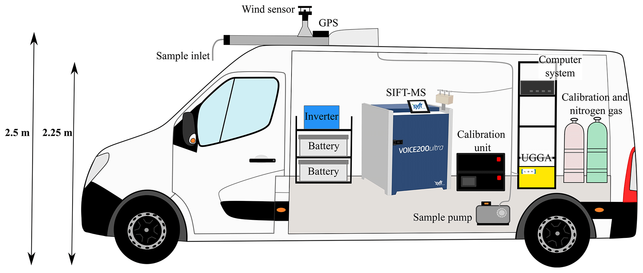
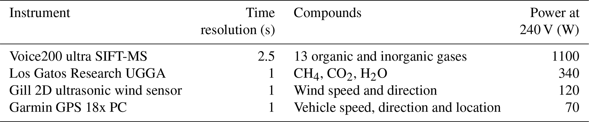
The front-facing sample inlet of the van sits at 2.25 m off the ground, at windscreen height of the WASP, and is made from a 6 m length of PTFE (Teflon) tubing with a diameter of 12.5 mm ( inch). Sample air is drawn from the outside through the sample inlet by a pump located in the rear at a flow rate of 40 SLPM and is then fed into the instruments mounted in the rear. Real-time location of the WASP is recorded by a Garmin GPS 18x PC, and wind speed and direction are measured using a Gill 2D ultrasonic wind sensor (which was not used in this study), both of which are fitted on the roof of the WASP at a height of 2.5 m. Data outputs of the roof sensors and the UGGA are stored on a computer system in the van, and the outputs of the SIFT-MS are stored in the internal system of the instrument. Ethernet port connections between the computer system and the SIFT-MS mean that data for all of the instruments can be visualised in real time in the driver cab whilst measurements are carried out. A schematic of the WASP is shown in Fig. 1, and further details of the instrumentation are provided in Table 1. Note that the instrument fit in the WASP is flexible and easily altered due to the relatively large size and payload that the WASP can accommodate.
2.2 Instrumentation
2.2.1 Selected-ion flow-tube mass spectrometer (SIFT-MS)
A Voice200 ultra SIFT-MS manufactured by Syft Technologies (Christchurch, New Zealand) was used to quantify VOCs and inorganic gases. The SIFT-MS principles of operation are discussed in detail elsewhere (Smith and Spanel, 1996; Smith and Španěl, 2005), but a brief outline is included here. The instrument consists of a switchable reagent ion source capable of rapidly switching between multiple reagent ions: H3O+, NO+ and , which are generated in a microwave plasma ion source from a mixture of air and water at a pressure of approximately 440 mTorr. The reagent ions are then extracted into the upstream quadrupole chamber maintained at a pressure of approximately Torr using a 70 L s−1 turbo-molecular pump and then pass through an array of electrostatic lenses and the upstream quadrupole mass filter. Those not rejected by the mass filter are injected into the flow tube where they are thermalised in a stream of nitrogen prior to selectively ionising target analytes. The product ions then flow into the downstream quadrupole mass filter and the secondary electron multiplier detector, where the ions are separated by their mass-to-charge ratios () and the ion counts are measured. The mixing ratios of analyte compounds in the flow tube are calculated using the ion–molecule reactions that take place within the SIFT-MS using Eq. (1), where [A] is the analyte mixing ratio, γ is the instrument calibration factor, [P+] is the product ion, [R+] is the reagent ion, tr is the reaction time and k is the rate constant.
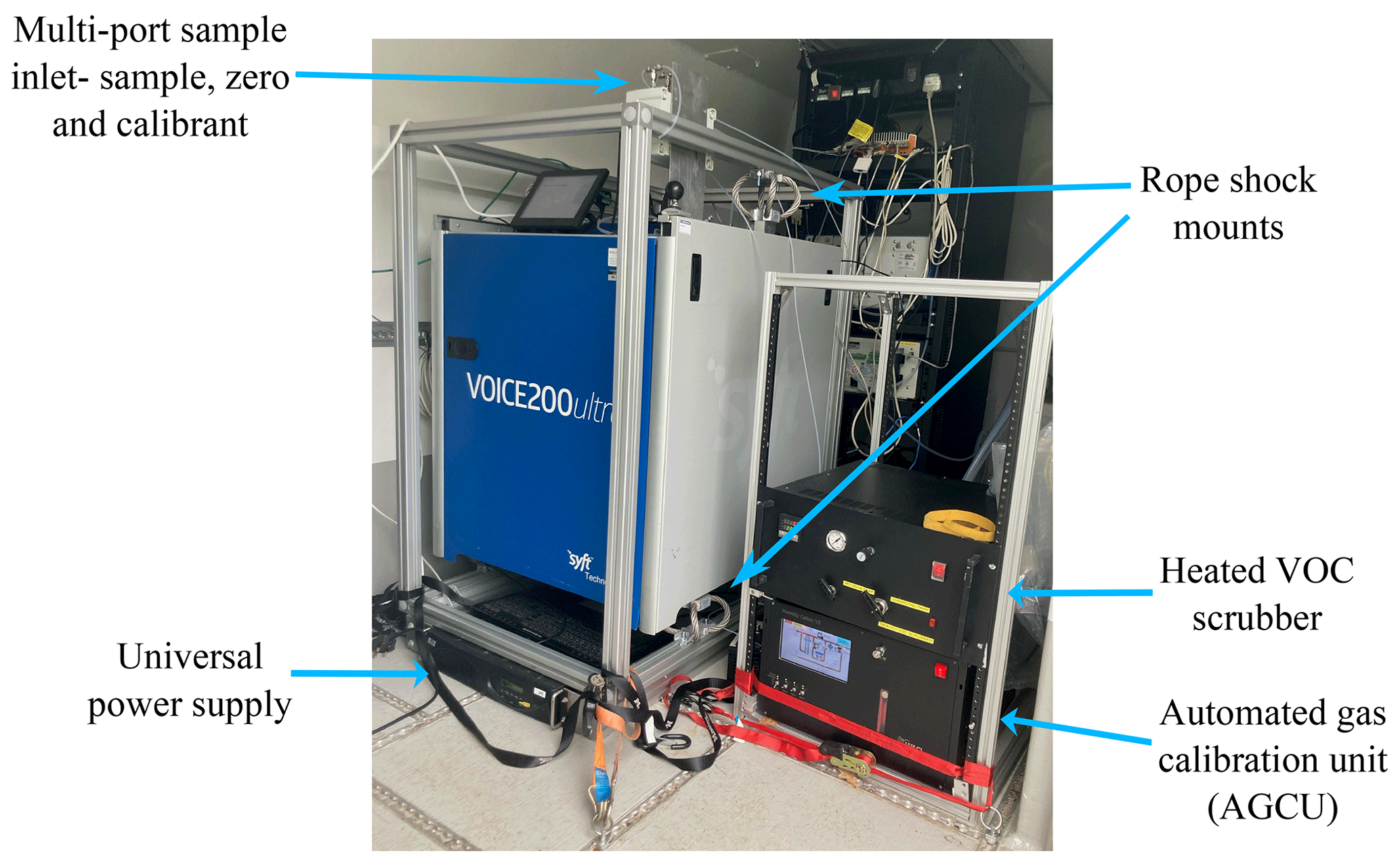
Figure 2The Voice200 ultra SIFT-MS with in-house-built multi-port inlet and heated VOC scrubber, alongside the custom-built automated gas calibration unit (AGCU).

Figure 3Schematic of the internal gas flow paths in the automated gas calibration unit (AGCU).
Figure 2 shows the SIFT-MS inside the WASP, with an in-house multi-port sample inlet capable of autonomously selecting between sample, zero and calibrant gases using the instrument software (Labsyft 1.6). The multi-port inlet uses three PTFE internally coated solenoid valves (12VDC, Gems). The SIFT-MS is suspended in a rope-shock mounted rack, which reduces the three-dimensional vibration the instrument is subjected to during mobile measurements. Whilst driving, the SIFT-MS was operated using a flow-tube pressure of 460 mTorr, a nitrogen carrier gas (Research grade, BOC) with a flow rate of 0.6 Torr L s−1 and a sample flow rate of 100 SCCM. On the right in Fig. 2 is a custom-built automated gas calibration unit (AGCU) and a heated VOC zero air generator. The heated VOC scrubber consists of palladium-coated alumina pellets heated to 380 ∘C, which produces zero air whilst maintaining the humidity of the sample gas. Mass flow controllers (MFCs) (Alicat) in the AGCU measure and control the flows of diluent zero air and the VOC standard (1 ppm certified National Physical Laboratory, UK), and they allow for controlled dilution ratios in the parts per trillion to parts per million (ppt–ppm) range. Automated stepwise changes to the dilution ratios are made, which generates a multi-point calibration curve for routine external calibration of the SIFT-MS. Figure 3 shows a simplified schematic of the internal gas flow paths in the AGCU, and calibration of the compounds is discussed further in Sect. 3.1.
Table 2The compounds measured by the SIFT-MS and their corresponding reagent ions, molecular masses and product ion chemical formulas.
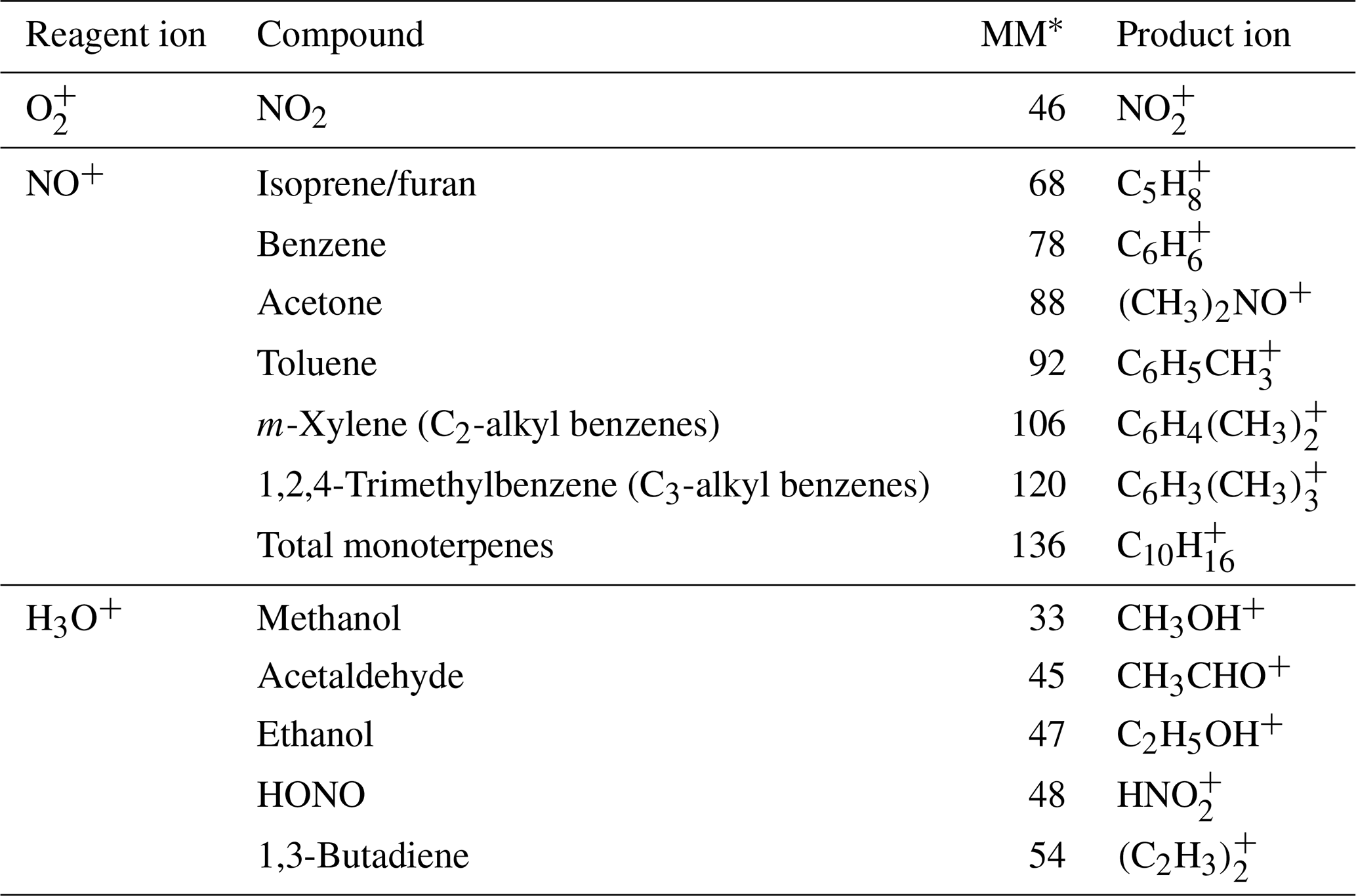
∗ Molar mass in g mol−1.
The SIFT-MS was used to measure 13 different VOCs and inorganic gases during mobile measurements around the city of York, UK. The compounds targeted with the SIFT-MS were chosen to cover a range of emissions sources to help with source apportionment analysis. The compounds measured by the SIFT-MS and the corresponding reagent ions, molecular masses and product ion chemical formulas are shown in Table 2. To maximise spatial data density during mobile measurements, the instrument acquisition rate was minimised with only a single product ion monitored for each compound. Therefore, the sampling method used during measurements has an acquisition rate of 2.5 s with a 90 ms ion dwell time.
2.2.2 Ultra-portable greenhouse gas analyser (UGGA)
A Los Gatos Research ultra-portable greenhouse gas analyser (UGGA) was used to quantify carbon dioxide (CO2), methane (CH4) and water vapour (H2O). The UGGA instrument uses off-axis integrated-cavity output spectroscopy (off-axis ICOS) to quantify mixing ratios of gaseous species, which has been described in detail previously (Gupta, 2012), but a brief description is included here. Off-axis ICOS uses a laser and an optical cavity in an off-axis configuration (Tan and Long, 2010), which enhances the measured absorption of light by a sample by creating an effective optical path length of several thousand metres. The measured absorption spectrum is recorded, and when this is combined with the measured gas temperature and pressure in the cell, effective path length and known line strength, it can be used to determine a quantitative measurement of mixing ratio.
The UGGA was used at a 1 Hz time resolution, with a response time of 10 s. The precision of the UGGA over 1 s is 2 ppb for CH4 and 500 ppb for CO2, and the limit of detection (LoD) is 3 ppb for CH4 and 800 ppb for CO2. The precision and LoD of the UGGA were calculated using 2σ and 3σ, respectively, of gas-canister-only measurements made whilst driving. The measurement range of the UGGA is 0.01–100 and 1–20 000 ppm for CH4 and CO2, respectively. A quantitative measurement of mixing ratio could be determined directly from the UGGA without the need for calibration during each drive, but the UGGA was calibrated with external gas cylinders before and after the measurement period.
2.3 Measurement location
In the summer of 2020, the WASP was used to make measurements around the city of York, UK. Figure 4 shows the measurement route that was driven by the WASP. The route starts at the University of York and then passes into and around the inner ring road of the city and has a total distance of 15.1 km. York has a population of approximately 200 000 people, and air pollution in the city is thought to be dominated by vehicle emissions, especially around the inner ring road, due to congestion. The measurement route in York was designed to capture a variety of potential emissions sources, such as hairdressers, beauty salons, dry cleaners and eateries, to determine dominant sources. Measurements were carried out for a total of 10 d between 30 June and 23 July 2020 during periods of dry weather between the hours of 10:00 and 17:00 BST. The route was driven 30 times in total, and the dates and times of each drive are included in the Appendix (Table A1). It should be noted that during the measurement period the COVID-19 stringency index was 64.35 (taken from Our World in Data, 2021), indicating reduced economic and traffic activity. This could affect both the concentration and detection of different VOC species due to possible decreased emissions.
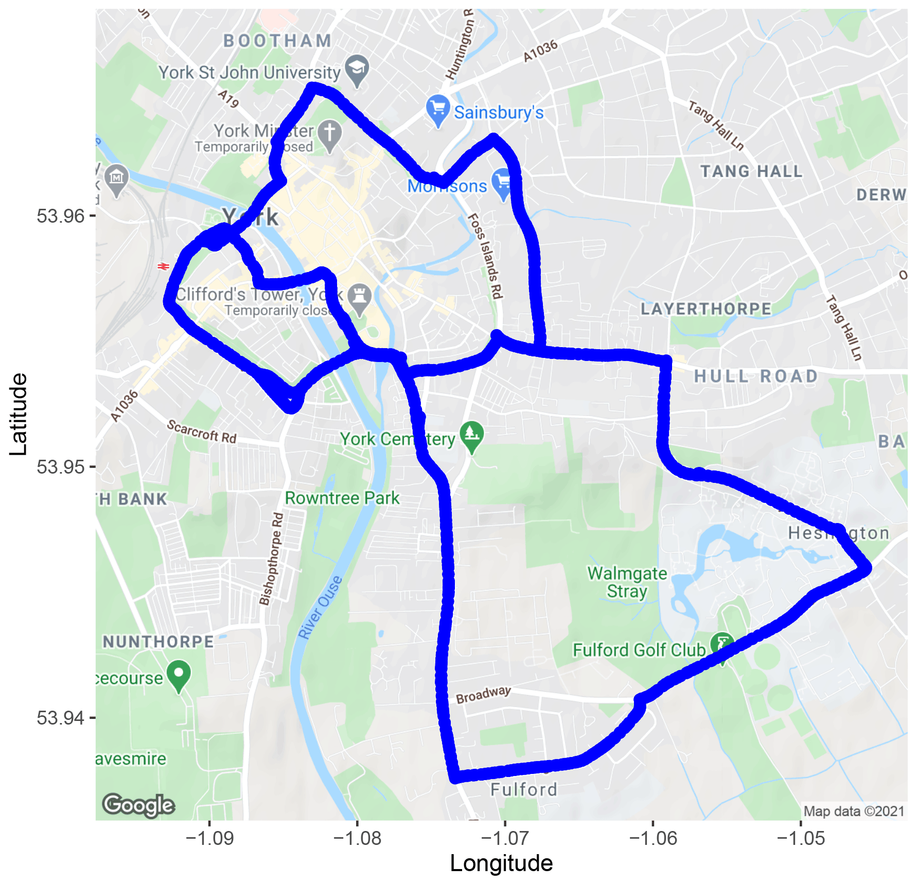
Figure 4Measurement route driven by the WASP for mobile measurements around York (© Google). Visualised by the ggmap R package (Kahle and Wickham, 2013).
3.1 Calibration and data quality assurance
The mixing ratios of all of the compounds measured by the SIFT-MS were dependent on the compound-specific rate constant and daily generated instrument calibration factor (ICF – γ, Eq. 1). The daily ICF was derived using a 2 ppm gas standard to validate the mass-dependent ion transmission of the instrument; details of the gas standard are included in the Appendix in Table A2. A zero offset was applied for all of the compounds, which was taken from zero air for VOCs and from a nitrogen blank for other compounds, such as HONO and NO2. In the case of acetaldehyde, total monoterpenes, NO2 and HONO, the mixing ratios were determined directly from the daily ICF. The remaining compounds were externally calibrated using the automated gas calibration unit (AGCU, discussed in Sect. 2.2.1) and a 1 ppm 14-component VOC gas standard (National Physical Laboratory). These compounds include acetone, benzene, butadiene, ethanol, isoprene, methanol, m-xylene (C2-alkyl benzenes), toluene and trimethylbenzene (C3-alkyl benzenes). Figure 5 shows the multi-point calibration of these compounds, which was carried out at the start and end of each day (pre- and post-drive). Both pre- and post-drive SIFT-MS calibrations were performed to ensure specific VOC compound sensitivities did not change during mobile operation. Due to operational time constraints associated with switching on the SIFT-MS at the start and end of each day, the chosen calibration procedure had to be as concise as possible. In order to assess both intra- and inter-calibration reproducibility daily, duplicate calibration steps were carried out both before and after mobile operation. The calibrations were performed at VOC mixing ratios of 10, 5, 1 and 0 ppb, and each of the mixing ratio steps lasted for 3 min.
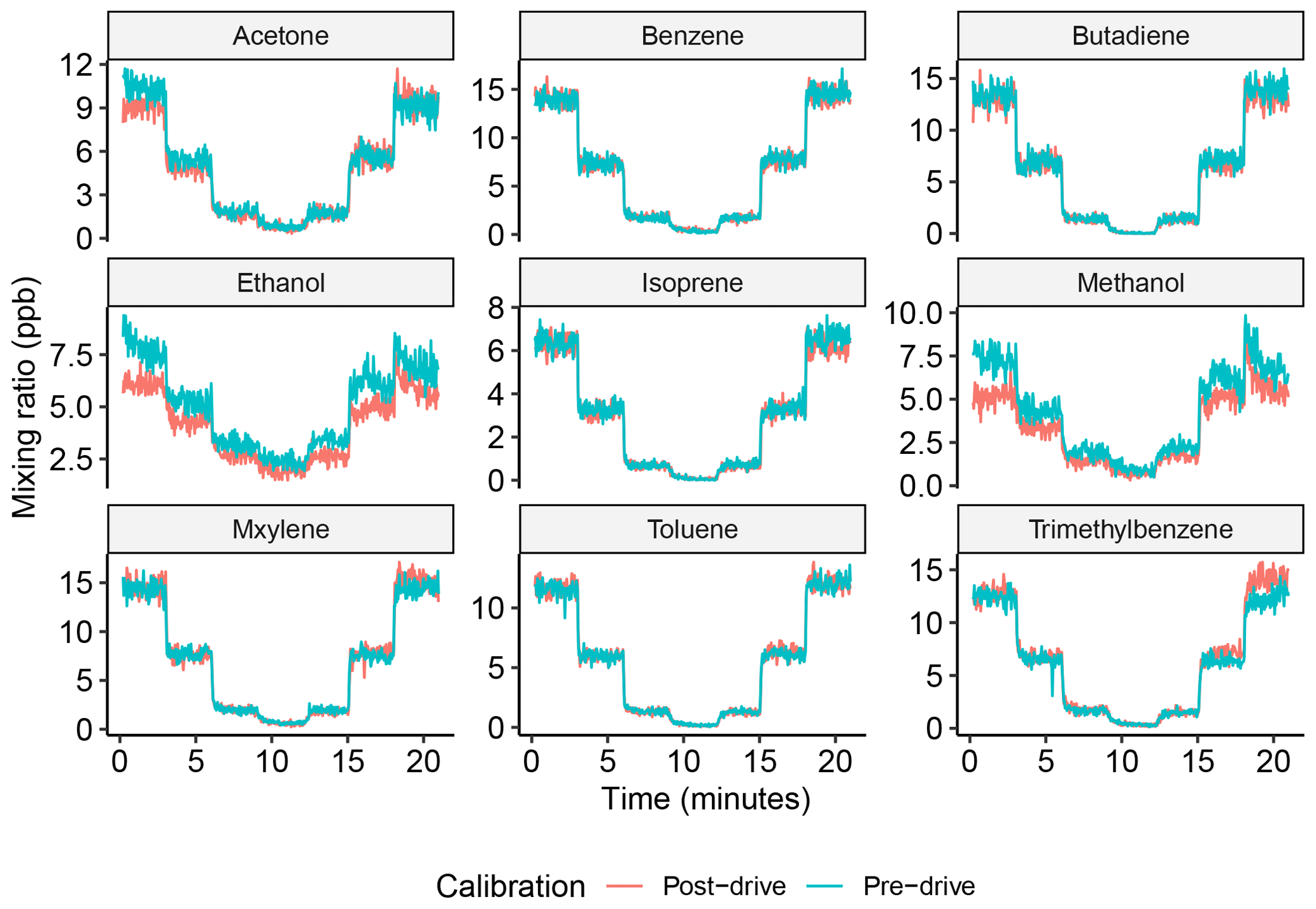
Figure 5Multi-point calibration for VOC gas standard compounds over 10, 5, 1 and 0 ppb. The blue line shows the calibrations performed pre-drive, and the pink line shows the calibration performed post-drive.
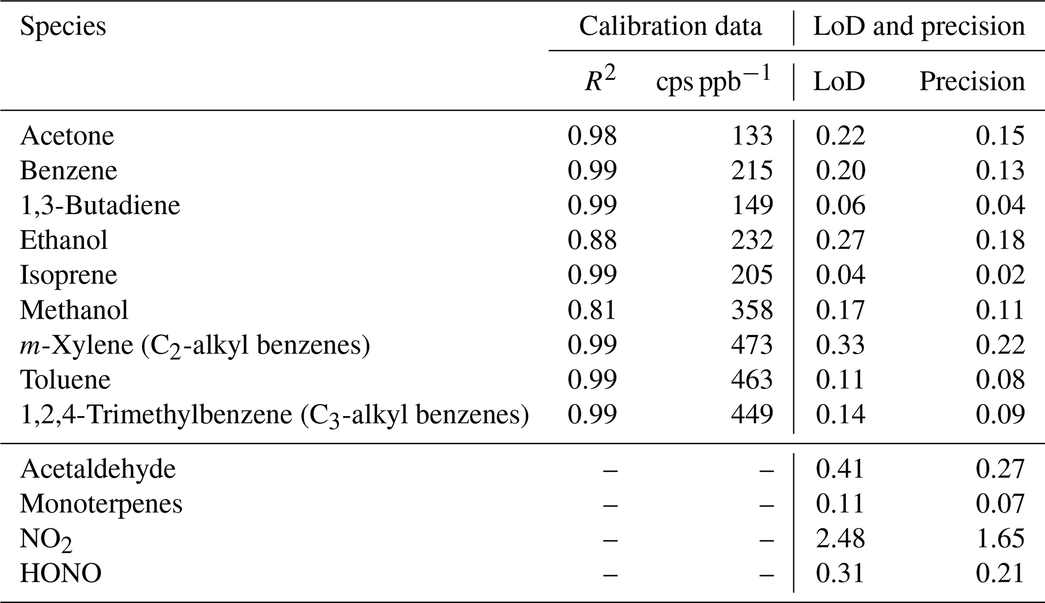
Table 3The coefficient of determination (R2) and the ion counts per second per part per billion (cps ppb−1) calculated from the SIFT-MS calibrations. The limit of detection (LoD) and precision of compounds measured by the SIFT-MS (in ppb) for every 2.5 s measurement. Compounds in the upper part of the table were externally calibrated.
The left- and right-hand steps of the calibrations showed good agreement (as shown in Fig. 5). The left-hand calibration steps were used to condition the internal surfaces and SIFT-MS inlet and were therefore not used for calibration. Compound-specific calibration curves were obtained from the average of the last minute of each 3 min right-hand step of the post-drive calibrations, and data influenced by mixing ratio transitions were removed. Calibrations were carried out daily, and results were applied to the mixing ratio data obtained during mobile measurements. Figure 5 also shows good agreement for the majority of the compounds between the pre- and post-drive calibrations, and differences in the mixing ratios may have been due to changes in ambient temperature, as pre-drive calibrations were usually performed in the morning when the temperature was lower. This may have led to the alcohols sticking on the sample lines or mixing with condensation in the line during calibrations. Additional data from the calibrations, including the coefficient of determination (R2) values and ion counts per second per part per billion (cps ppb−1), are included in Table 3.
Table 3 shows the precision and the limit of detection (LoD) for the SIFT-MS compounds, which were calculated using 2 (precision) and 3 (LoD) times the standard deviation (σ) of measurements made when sampling zero air or nitrogen gas. The precision and the LoD shown in Table 3 were calculated over 2.5 s, which is the acquisition rate of the SIFT-MS measurements.
To ensure that the VOC mixing ratios measured by the SIFT-MS were independent of instrumental noise, instrument dark counts using the H3O+ reagent ion ( 25) were routinely measured during mobile operation, which is shown in the Appendix (Fig. A1) along with benzene concentration and counts per second (cps) for the benzene product ion ( 78). There was typically minimal instrument noise (0–40 cps for 25) observed during a 45 min mobile measurement period. Furthermore, significant increases in the mixing ratio of benzene corresponded to large increases in 78 (>40 cps), therefore showing that these were due to real increases in ambient concentrations. Periods of elevated noise (>100 cps) were routinely removed to improve measurement accuracy. During the 10 d of measurements, a total of approximately 26.5 h of measurements were made and only 3 min of the measurements had to be removed due to excess instrument noise, which may have been due to extreme vibrations or movement when driving. Movement and vibration effects on instrument noise whilst driving were further investigated by sampling the SIFT-MS instrument on nitrogen only, which is shown in the Appendix (Fig. A2). The run did not show any significant changes in instrument noise whilst driving, and there were no increases in compound mixing ratios, therefore showing that the driving motion had only a minimal effect on measurement accuracy.
3.2 Summary of measurements and spatial distribution
Figure 6 shows a statistical summary of the mobile measurements carried out in York in a box-and-whisker plot. The plot shows that butadiene, isoprene, HONO and monoterpene mixing ratios were consistently below 0.5 ppb, suggesting a lack of emission sources for these compounds in York, either generally or as a result of COVID-19 restrictions. The majority of the measurements of butadiene and HONO were below the limit of detection, so these compounds are not to be included in any further analysis. For the other compounds there is greater variation in the mixing ratios. The greatest variation for compounds measured by SIFT-MS is seen for vehicle-emissions-related compounds, such as benzene, toluene, m-xylene and NO2, in addition to other species such as acetaldehyde and ethanol. The variation in ethanol may also be related to emissions from vehicles or fuel evaporation due to ethanol addition in gasoline fuel. Ethanol variation could also result from use of VCPs. Acetaldehyde variation may be due to emissions from vehicles as an oxidation product or other atmospheric processes. It is difficult to say exactly what emissions source is responsible for the variation in ethanol and acetaldehyde, but methods such as spatial mapping, correlation and ratio analysis can be used to investigate different sources. It is still worth noting that the variation of all of the compounds is still small, which is likely due to COVID-19 restrictions and reduced economic and traffic activities around York. The majority of the measurements (90.2 % – excluding butadiene and HONO) made by the SIFT-MS significantly exceeded the LoD calculated for each compound (Table 3), and the 30 m aggregated median concentrations used for spatial mapping were on average a factor of 2.2 higher than the LoD. This provides confidence that the observed compound peaks correspond to real increases in ambient concentrations. The typical spatial distance for the 2.5 s recorded by the SIFT-MS was 14 m as the average speed of the mobile laboratory was 20 km h−1 during measurements around York.
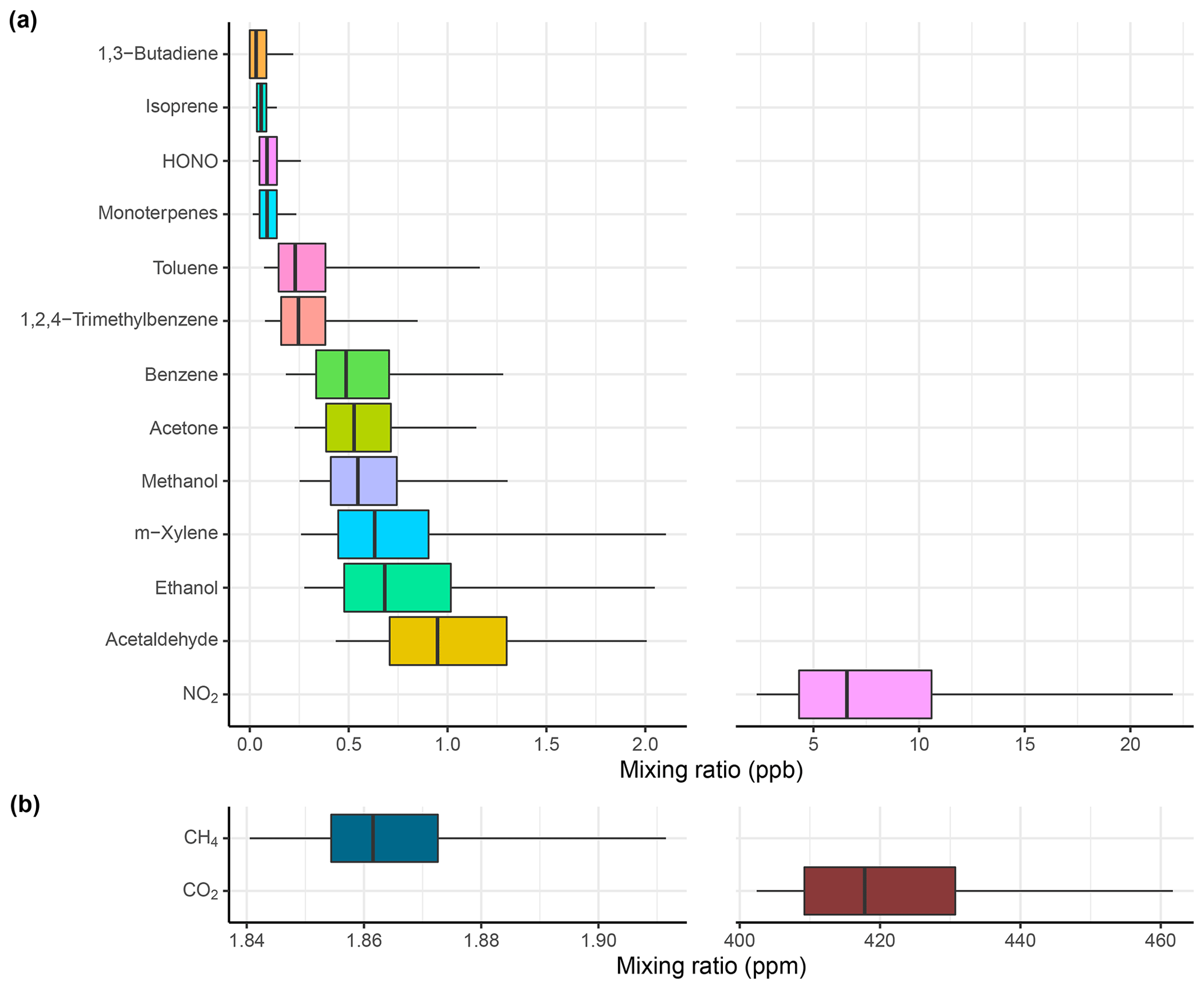
Figure 6Summary of measurements made by (a) the SIFT-MS (in ppb) and (b) the UGGA (in ppm) during 30 repeat drives around York. The box outline contains the 25th to the 75th percentile, and the middle line shows the median mixing ratio for each compound. The whiskers represent the 5th and 95th percentile for the mixing ratios of each compound. It is worth noting that NO2 and CO2 are on individual scales due to differing ranges in their mixing ratios.
To spatially map the measurements made by the WASP mobile laboratory the data points were “snapped” to the nearest 30 m segment of road using GPS data (Apte et al., 2017). The points in each 30 m segment of road were then aggregated to give the median value. The median was selected as it would represent a realistic picture of air pollution and emissions sources on the measurement route and remove any biases that may occur from directly sampling vehicle exhaust.
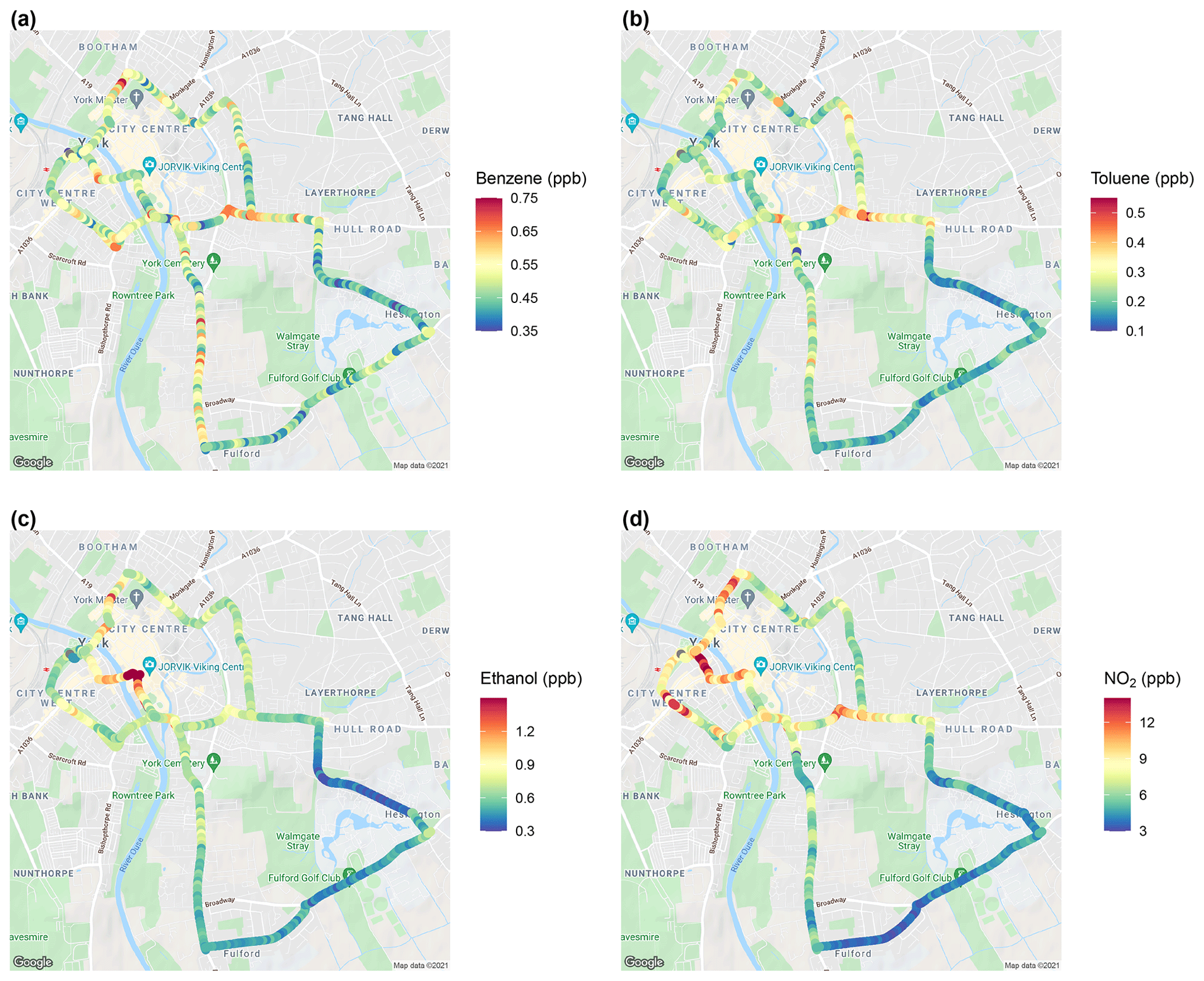
Figure 7Spatial mapping of median values of (a) benzene (ppb), (b) toluene (ppb), (c) ethanol (ppb) and (d) NO2 (ppb) from mobile measurements around York (© Google). Visualised by the ggmap R package (Kahle and Wickham, 2013).
Figure 7 shows the mixing ratios of benzene, toluene, ethanol and NO2 recorded along the York measurement route as examples of spatial mapping of compounds using the WASP and the SIFT-MS. The plot shows low mixing ratios on Heslington Lane (blue–green at the bottom of Fig. 7) for all of the compounds. The mixing ratios increase around the city centre, where there is higher congestion and emissions may be dominated by vehicles. NO2 mixing ratios considerably increase in the city centre to above 12 ppb and elevated levels are seen at road junctions, which is expected as NO2 is strongly indicative of diesel vehicles. Particularly high levels of NO2 are observed past the train station and on roads with many bus stations. Increases in the median benzene and toluene mixing ratios are relatively small, but they show similarities to each other with some elevated levels at road junctions, which is indicative of emissions from road vehicles. Ethanol is at background levels for the majority of the route, with considerable increases seen in the city centre of above 1.2 ppb (red in the centre of the map), which may possibly originate from businesses in the city centre, such as bakeries and breweries. It is important to look at correlations of species with one another in order to determine sources of VOC compounds in York.
3.3 Spatial correlation mapping
Spatial mapping is useful as it can highlight hotspots of VOCs and trace gases, but they are insufficient in determining and separating emissions sources in urban areas. A method for source apportionment is to consider the correlation between many species over particular roads or areas that measurements have been made. Areas that contain different emissions sources should have different correlations; for example, an area dominated by vehicle emissions should show strong correlations with VOCs associated with vehicles such as benzene and toluene, and these correlations will be different to other sources, such as evaporative emission of solvents. Figure 8 shows the Spearman correlation of compounds for all of the measurements made by the SIFT-MS and UGGA in York.
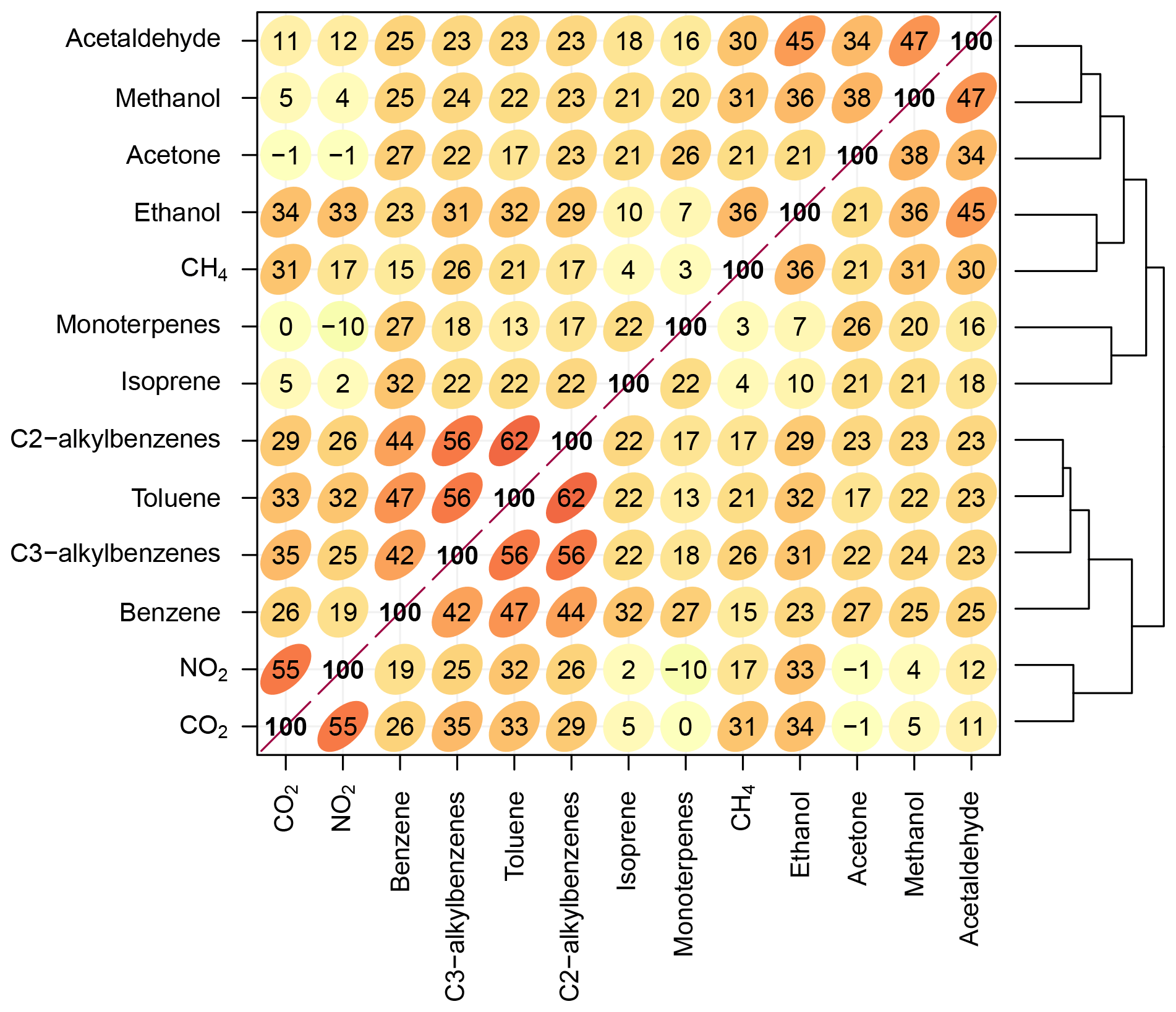
Figure 8Spearman correlation of the compounds measured using the WASP and the SIFT-MS during measurements in York. Note that hierarchical clustering is applied to the correlation matrices to group species that are most similar to one another. A higher correlation coefficient between species is represented by a higher number, a darker red colour and an ellipse (shape). The lines on the right-hand side show the hierarchical clustering between compounds and represent clusters of species with similar patterns and/or behaviours.
Hierarchical clustering is applied to the correlation matrices to group species that are most similar to one another. For example, benzene, toluene, C2-alkyl benzenes and C3-alkyl benzenes appear next to each other in Fig. 8 and show a clear cluster, indicating similar behaviour, likely related to their common sources of gasoline evaporation and engine exhaust emissions. There are other clusters of VOCs which are indicative of different source types – for example, commons solvents such as acetaldehyde, methanol and acetone are clustered together in linked urban emissions likely not relating to road transport. Other trace gases associated with tailpipe emissions also appear in a single cluster, e.g. NO2 and CO2. Ethanol is equally correlated with the vehicle-related cluster (benzene, toluene, C2-alkyl benzenes and C3-alkyl benzenes) and a non-vehicle-related cluster (acetaldehyde, methanol and acetone), indicating that the sources of ethanol in York are complex and that there is not one dominating emissions source. In the future, the aim is to apply this method to smaller spatial scales, at which it is expected that spatially varying patterns of correlation may enable specific emissions sources to be identified, potentially at the individual building scale.
The correlation plot shown in Fig. 8 is also useful as it can be used as a guide for further analysis. Correlations between species can be investigated on a smaller scale through ratio analysis using quantile regression, such as the toluene-to-benzene ratio, which will be discussed in Sect. 3.4.
3.4 Evaporative source characterisation
Determining the importance of different sources in the emissions of atmospheric pollutants is difficult, and calculating the ratios between compounds can be used as an indicator of dominating emissions sources. The toluene-to-benzene (T B) ratio has been used in many studies to determine the dominant source of these compounds, and it will be used here. Both toluene and benzene are emitted directly from vehicle exhaust and more widely by industry and may also be present due to evaporative emissions from fuels and solvents. Therefore, the T B ratio is a useful indicator of the relative importance of different sources. A T B ratio of 1–2 indicates a traffic influence (Langford et al., 2019; Simpson et al., 2020), and a T B ratio of over 2 indicates solvent or evaporative influences (Simpson et al., 2020).
A characteristic of mobile measurements is the transient nature of emission sources. For sources such as road vehicle exhaust, the measurements will depend on the traffic conditions, which are inherently variable. With repeat measurements, these variations can be averaged-out to reveal consistent spatial patterns (Apte et al., 2017), which is shown by the spatial maps in Fig. 7. Some sources can, however, be highly transient such as the evaporative emissions from road vehicle fuel stations. The emission source from fuel stations can be highly variable and can depend on many variables: for example, the number of vehicles being refuelled. Furthermore, these sources will be intermittently detected due to the prevailing wind direction. It will often be the case that no plume is detected because the wind is from the wrong direction.
In terms of concentration measurements, some source contributions may show as infrequent high concentrations (or ratios of concentrations) that have little or no effect on median values. Taking the median value of concentrations, as used by Apte et al. (2017) and in Fig. 7, will down-weight the contribution from less frequent, higher concentrations. Considering the median is useful when investigating consistent emissions sources, however, there is potentially important information and intermittent sources that can be missed.
As an example, we consider the T B ratio to be indicative of both road vehicle exhaust and potentially evaporative emissions. The T B ratio can be derived from the slope of an ordinary least squares (OLS) regression relating the two species. The linear regression ratio between toluene and benzene derived across all of the repeat drives per a 30 m segment of road is shown plotted on a map of York in Fig. 9. Figure 9 shows hotspots in the T B ratio of above 4 on Hull Road and James Street (which joins Hull Road, both of which are labelled). On Hull Road there are two road vehicle fuel stations, and on James Street there is an industrial area including a bus depot. The increased T B ratio along these roads is significant as it is continuously high for multiple 30 m segments. These two roads only account for about 5 % of the route and may represent an important source of toluene. However, OLS regression considers the mean response and does not capture the full distribution of relationships that exist between toluene and benzene across all 30 of the repeat drives. To address this issue we adopt quantile regression to provide increased distributional information.

Figure 9A spatial map showing the toluene-to-benzene (T B) ratio calculated using ordinary least squares (OLS) regression (© Google). The ratio was calculated using toluene and benzene measurements made during all 30 repeat drives around York, and each point represents the ratio for a 30 m segment of road. Elevated ratios on Hull Road and James Street are labelled with red arrows. Visualised by the ggmap R package (Kahle and Wickham, 2013).
While an OLS regression line minimises the distance of the trend line to each point of data, quantile regression attempts to define a line such that a certain proportion of the data is found above and below it (Koenker, 2021). For example, the median quantile regression slope would have 50 % of the data either side of it, whereas the slope associated with the 90th percentile would have 90 % of the data below and 10 % above. Through a quantile regression approach, the influence on the response variable by the predictor variable can be understood at different values of the response variable. The value and/or significance of a slope estimate could significantly vary between different quantiles. For example, a predictor variable may have a large influence on the response variable associated with “average” members of a population, but not those belonging to lower or higher quantiles. In the context of mobile measurements, high quantile values are used to explore the nature of transient evaporative sources that can be difficult to identify through OLS regression.
In a further development, rather than dividing the road network into discrete, non-overlapping 30 segments to calculate the T B ratio, a Gaussian kernel smoother is used. This approach has the advantage of providing a continuous weighting function that gives more weight to data close to the location of interest, while down-weighting data collected further away. The approach also avoids arbitrarily dividing the road up into sections, whereby it can be difficult to determine an appropriate section length. Additionally, the Gaussian kernel weighting can be used directly in quantile regression modelling (or other statistical models), effectively providing a continuous estimate of the T B ratio spatially, for different quantile values.

Figure 10The toluene-to-benzene (T B) ratio along the distance of Hull Road at quantiles of 0.99 (purple), 0.95 (dark blue), 0.9 (turquoise), 0.75 (green) and 0.5 (yellow) calculated using a Gaussian kernel smoother. The large peak at around 860 m corresponds to a road vehicle fuel station, indicating evaporative emissions from this source.
Figure 10 shows the results of the Gaussian kernel smoother along the distance of Hull Road at varying quantiles of 0.5, 0.75, 0.9, 0.95 and 0.99 using benzene and toluene measurements from all of the repeat drives. The plot shows that as the percentiles increase, so does the T B ratio. This is significant as the higher quantiles represent intermittent sources that would be missed by considering only the 50th percentile. While the median T B ratio peak is around 4, the higher quantiles (0.75 to 0.99) converge on a ratio closer to 7 or 8, which will be more representative of the intermittent evaporative source than the median slope value or the OLS regression slope. On Hull Road there is a road vehicle fuel station situated at around 860 m, which corresponds to the large increase in the T B ratio, and this is highly likely due to evaporative emissions from the fuel station due to the absence of other potential sources at this location.
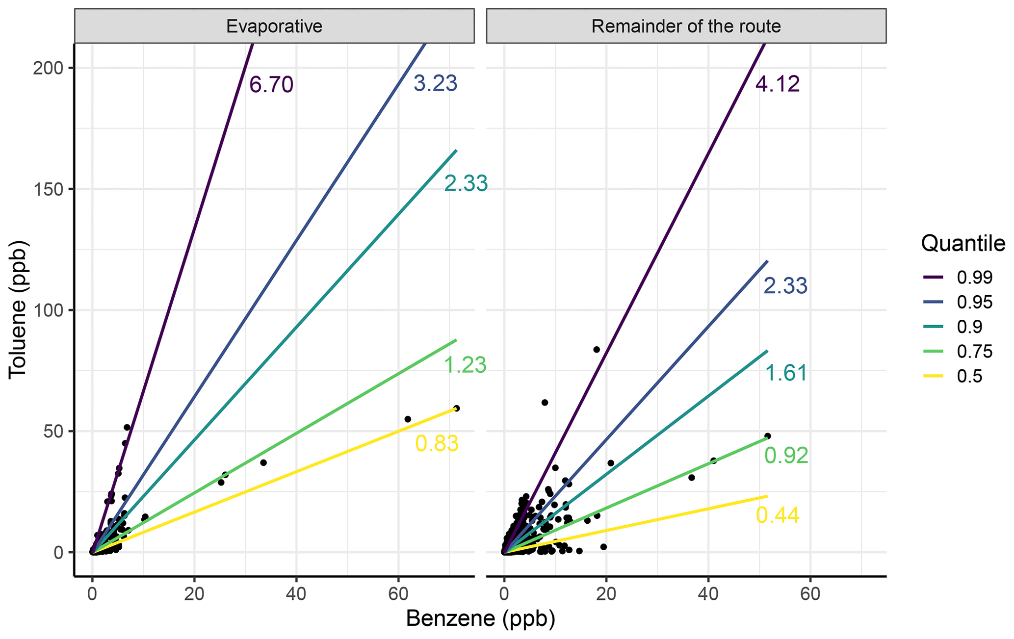
Figure 11The toluene-to-benzene (T B) ratio for the evaporative areas (Hull Road and James Street) and for the remainder of the route at quantiles of 0.99 (purple), 0.95 (dark blue), 0.9 (turquoise), 0.75 (green) and 0.5 (yellow), with the corresponding slope values also displayed. The toluene and benzene values for each of the comparative figures were produced using data collected from all 30 repeat measurement drives.
Figure 11 shows a comparison of the T B ratio for the roads with a higher T B ratio (Hull Road and James Street) – labelled as evaporative – and the remainder of the route. Figure 11 shows that at higher quantiles, the evaporative area has a much higher T B ratio than the remainder of the route (6.70 compared to 4.12) but that it is still significant and corresponds to an intermittent source. The figure also shows that at lower quantiles of 0.5 and 0.75, both of the comparison plots agree well, with similar T B ratios, representing emissions from vehicle exhausts. These results suggest that on the whole route, there is only a minor contribution of evaporative sources (about 5 % of the length) that can clearly be identified in the data. Extending the route in York or making measurements in other urban areas with a wider range of source types would help develop these methods further.
The SIFT-MS has been used to perform high temporal and spatial measurements of multiple VOCs in an urban area, and we present some examples of this. The spatial mapping examples highlight the use of the SIFT-MS to reveal hotspots of pollutants that can be investigated by further measurements in that area or through analysis, which helps to reveal emissions sources. The correlations of species have been shown using a correlation matrix alongside hierarchical clustering, which groups species dependent on their similarities and can be used to determine emissions sources of certain species. Correlations between species can be used to determine further analysis for the measurements made by the SIFT-MS in the mobile laboratory. For example, compound correlations can be further investigated through ratio analysis, which can be indicative of specific emissions sources. We have investigated the toluene-to-benzene ratio to determine the influence of different sources on their emissions. Gaussian kernel weighting was directly used in quantile regression modelling to provide an estimate of the T B ratio spatially, which indicated evaporative emissions at higher quantile values. These methods will be further developed in the future for source apportionment and characterisation of different source types along the whole of the York route, which can be used to increase understanding of air pollution in urban areas and for future emissions regulations.
A UV photometric O3 instrument will be added together with an ICAD NOx instrument, which will make for good comparison to the SIFT-MS-measured NO2. Future applications will be to return to measurements around York once travel activities return to normal, as the current COVID-19 situation appears to have had an effect on air pollution during the measurement period due to decreased traffic and closed facilities. The upgrades discussed here highlight the potential to investigate vehicle emissions as the use of the SIFT-MS allows for direct measurements of high-concentration tailpipe emissions and for investigation of currently unregulated pollutants from vehicles. Future experiments investigating vehicle emissions include plume chase, whereby the mobile laboratory would follow a vehicle and sample the exhaust emissions for a period of time, and individual vehicle exhaust plume sampling using the laboratory alongside remote sensing instruments by the side of the road and sampling vehicles as they pass. Additionally, direct measurements from the tailpipe will be used to highlight compounds of interest that can then be targeted by the SIFT-MS.
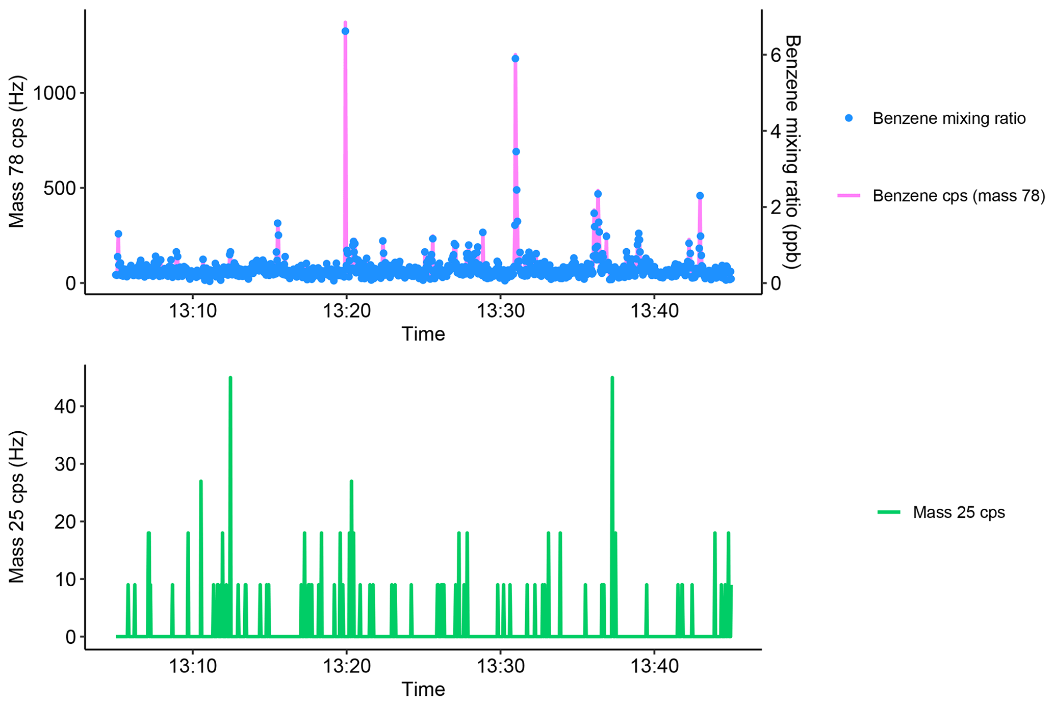
Figure A1Example of instrument noise during mobile measurements. The blue points show the mixing ratio of benzene, and the pink line shows the corresponding counts per second for the benzene ion counts per second (mass 78). The green line shows the variation of mass 25 during mobile measurements, which does not contain any periods of elevated noise.
Table A1Details of the number of times the route was driven each day and the times that the drives took place. Time zone is BST.
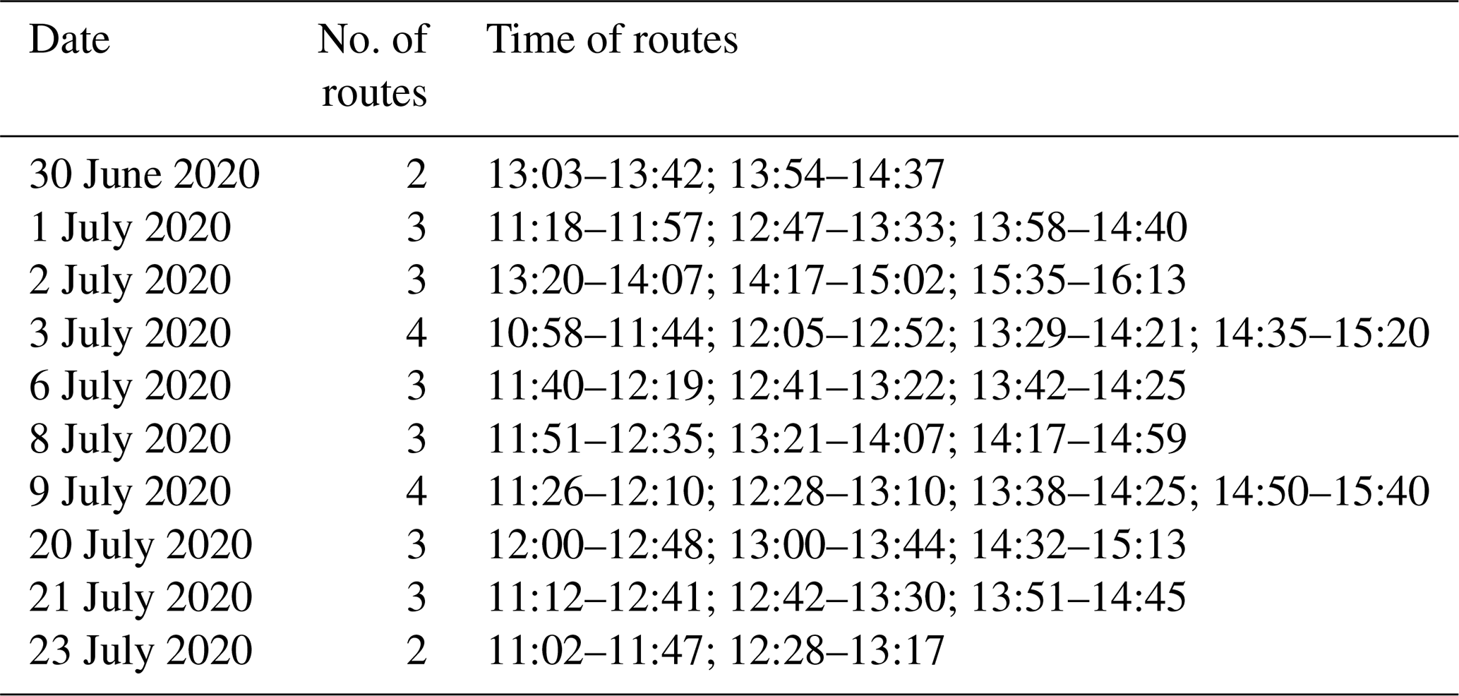
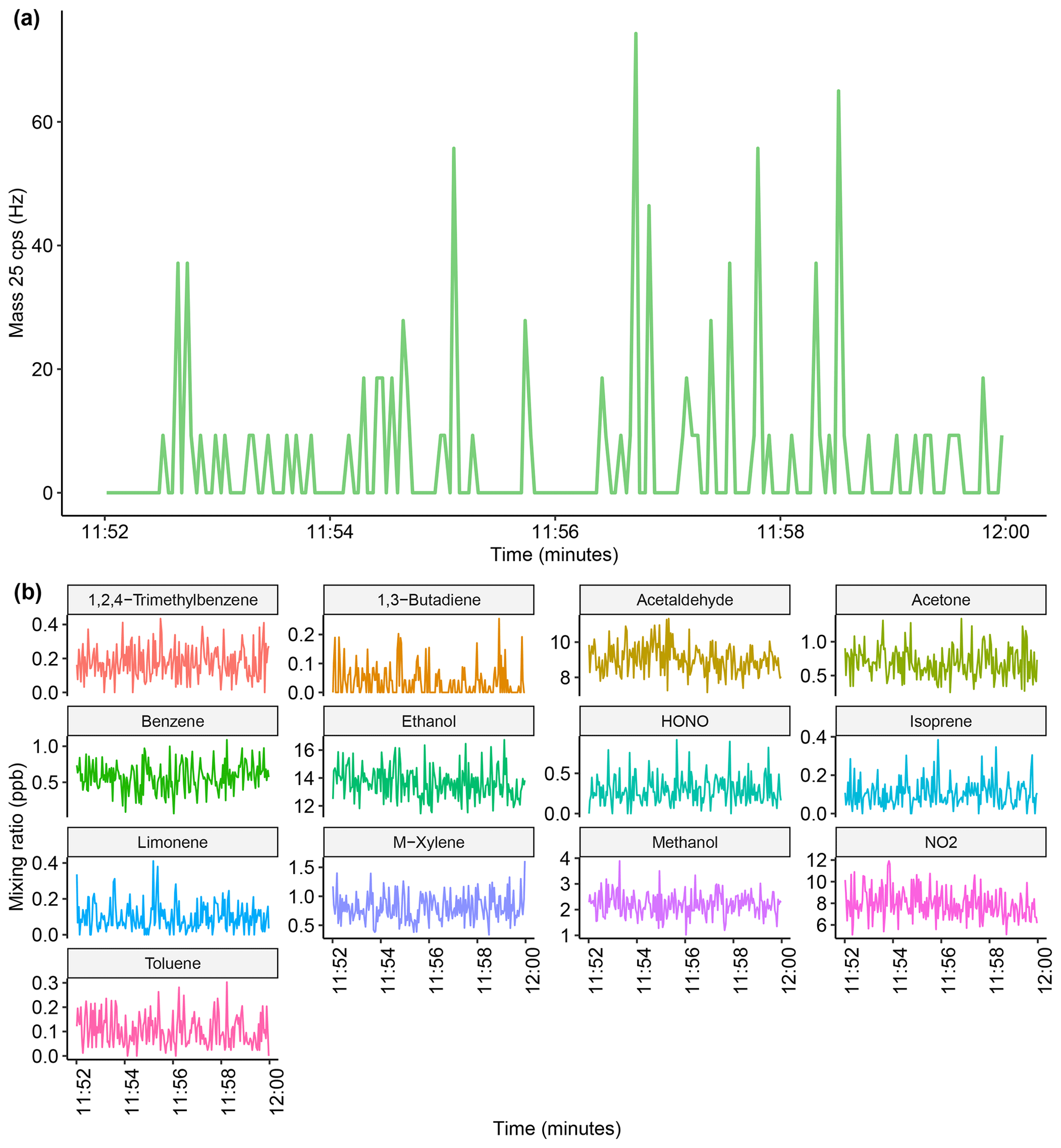
Figure A2(a) Counts per second of mass 25, which represents instrument noise, and (b) mixing ratios of the compounds during a nitrogen-only mobile measurement.
Table A2Compounds and their molecular masses in the Syft 2 ppm standard gas, which was used to generate the daily instrument calibration factor (ICF).
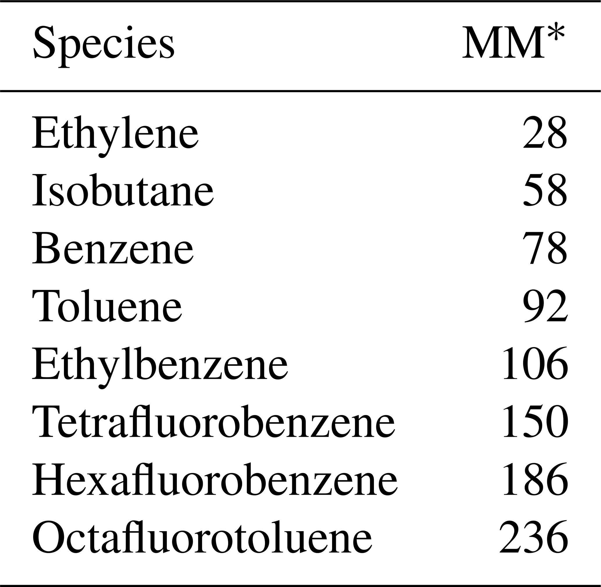
∗ Molar mass in g mol−1.
All data sets used and produced for the purposes of this work are available upon request from the corresponding author.
RLW prepared the paper with contributions from all co-authors. RLW and MDS designed and carried out the measurements. ACL, JRH and SY designed and built the mobile laboratory. DCC, NJF and JD assisted with data analysis and scientific discussion.
The authors declare that they have no conflict of interest.
Publisher's note: Copernicus Publications remains neutral with regard to jurisdictional claims in published maps and institutional affiliations.
The authors would also like to thank Stuart Grange and Shona Wilde for help with data analysis and visualisation. We would also like to thank Chris Anthony for driving of the WASP around York.
This research has been supported by the NERC Panorama Doctoral Training Partnership (grant no. NE/S007458/1).
This paper was edited by Anna Novelli and reviewed by two anonymous referees.
Our World in Data: COVID-19: Stringency Index, available at: https://ourworldindata.org/grapher/covid-stringency-index?tab=chart&country=~GBR, last access: 1 June 2021. a
Alas, H. D. C., Weinhold, K., Costabile, F., Di Ianni, A., Müller, T., Pfeifer, S., Di Liberto, L., Turner, J. R., and Wiedensohler, A.: Methodology for high-quality mobile measurement with focus on black carbon and particle mass concentrations, Atmos. Meas. Tech., 12, 4697–4712, https://doi.org/10.5194/amt-12-4697-2019, 2019. a
Apte, J. S., Messier, K. P., Gani, S., Brauer, M., Kirchstetter, T. W., Lunden, M. M., Marshall, J. D., Portier, C. J., Vermeulen, R. C., and Hamburg, S. P.: High-Resolution Air Pollution Mapping with Google Street View Cars: Exploiting Big Data, Environ. Sci. Technol., 51, 6999–7008, https://doi.org/10.1021/acs.est.7b00891, 2017. a, b, c, d
Ars, S., Vogel, F., Arrowsmith, C., Heerah, S., Knuckey, E., Lavoie, J., Lee, C., Pak, N. M., Phillips, J. L., and Wunch, D.: Investigation of the spatial distribution of methane sources in the greater Toronto area using mobile gas monitoring systems, Environ. Sci. Technol., 54, 15671–15679, https://doi.org/10.1021/acs.est.0c05386, 2020. a
Bush, S. E., Hopkins, F. M., Randerson, J. T., Lai, C.-T., and Ehleringer, J. R.: Design and application of a mobile ground-based observatory for continuous measurements of atmospheric trace gas and criteria pollutant species, Atmos. Meas. Tech., 8, 3481–3492, https://doi.org/10.5194/amt-8-3481-2015, 2015. a, b
Castada, H. Z. and Barringer, S. A.: Online, real-time, and direct use of SIFT-MS to measure garlic breath deodorization: a review, Flavour Frag. J., 34, 299–306, https://doi.org/10.1002/ffj.3503, 2019. a
Coggon, M. M., Veres, P. R., Yuan, B., Koss, A., Warneke, C., Gilman, J. B., Lerner, B. M., Peischl, J., Aikin, K. C., Stockwell, C. E., Hatch, L. E., Ryerson, T. B., Roberts, J. M., Yokelson, R. J., and de Gouw, J. A.: Emissions of nitrogen-containing organic compounds from the burning of herbaceous and arboraceous biomass: Fuel composition dependence and the variability of commonly used nitrile tracers, Geophys. Res. Lett., 43, 9903–9912, https://doi.org/10.1002/2016GL070562, 2016. a
Coggon, M. M., McDonald, B. C., Vlasenko, A., Veres, P. R., Bernard, F., Koss, A. R., Yuan, B., Gilman, J. B., Peischl, J., Aikin, K. C., Durant, J., Warneke, C., Li, S. M., and De Gouw, J. A.: Diurnal Variability and Emission Pattern of Decamethylcyclopentasiloxane (D5) from the Application of Personal Care Products in Two North American Cities, Environ. Sci. Technol., 52, 5610–5618, https://doi.org/10.1021/acs.est.8b00506, 2018. a
Crilley, L. R., Kramer, L. J., Ouyang, B., Duan, J., Zhang, W., Tong, S., Ge, M., Tang, K., Qin, M., Xie, P., Shaw, M. D., Lewis, A. C., Mehra, A., Bannan, T. J., Worrall, S. D., Priestley, M., Bacak, A., Coe, H., Allan, J., Percival, C. J., Popoola, O. A. M., Jones, R. L., and Bloss, W. J.: Intercomparison of nitrous acid (HONO) measurement techniques in a megacity (Beijing), Atmos. Meas. Tech., 12, 6449–6463, https://doi.org/10.5194/amt-12-6449-2019, 2019. a
Edie, R., Robertson, A. M., Soltis, J., Field, R. A., Snare, D., Burkhart, M. D., and Murphy, S. M.: Off-Site Flux Estimates of Volatile Organic Compounds from Oil and Gas Production Facilities Using Fast-Response Instrumentation, Environ. Sci. Technol., 54, 1385–1394, https://doi.org/10.1021/acs.est.9b05621, 2020. a
Gkatzelis, G. I., Coggon, M. M., McDonald, B. C., Peischl, J., Aikin, K. C., Gilman, J. B., Trainer, M., and Warneke, C.: Identifying Volatile Chemical Product Tracer Compounds in U.S. Cities, Environ. Sci. Technol., 55, 188–199, https://doi.org/10.1021/acs.est.0c05467, 2021a. a
Gkatzelis, G. I., Coggon, M. M., Mcdonald, B. C., Peischl, J., Gilman, J. B., Aikin, K. C., Robinson, M. A., Canonaco, F., Prevot, A. S., Trainer, M., and Warneke, C.: Observations Confirm that Volatile Chemical Products Are a Major Source of Petrochemical Emissions in U.S. Cities, Environ. Sci. Technol., 55, 4343, https://doi.org/10.1021/acs.est.0c05471, 2021b. a
Grulke, N. E. and Heath, R. L.: Ozone effects on plants in natural ecosystems, Plant Biol., 22, 12–37, https://doi.org/10.1111/plb.12971, 2020. a
Gupta, M.: Cavity-Enhanced Laser Absorption Spectrometry for Industrial Applications, Gases & Instrumentation International, 23–29, available at: http://www.lgrinc.net/documents/Cavity-Enhanced Laser Absorption Spectrometry for Industrial Applications May_June 2012.pdf (last access: 8 February 2021), 2012. a
Heald, C. L., Jacob, D. J., Fiore, A. M., Emmons, L. K., Gille, J. C., Deeter, M. N., Warner, J., Edwards, D. P., Crawford, J. H., Hamlin, A. J., Sachse, G. W., Browell, E. V., Avery, M. A., Vay, S. A., Westberg, D. J., Blake, D. R., Singh, H. B., Sandholm, S. T., Talbot, R. W., and Fuelberg, H. E.: Asian outflow and trans-Pacific transport of carbon monoxide and ozone pollution: An integrated satellite, aircraft, and model perspective, J. Geophys. Res.-Atmos., 108, 4804, https://doi.org/10.1029/2003JD003507, 2003. a
Herndon, S. C., Jayne, J. T., Zahniser, M. S., Worsnop, D. R., Knighton, B., Alwine, E., Lamb, B. K., Zavala, M., Nelson, D. D., McManus, J. B., Shorter, J. H., Canagaratna, M. R., Onasch, T. B., and Kolb, C. E.: Characterization of urban pollutant emission fluxes and ambient concentration distributions using a mobile laboratory with rapid response instrumentation, Faraday Discuss., 130, 327–339, https://doi.org/10.1039/b500411j, 2005. a
Kahle, D. and Wickham, H.: ggmap: Spatial Visualization with ggplot2, R J., 5, 144–161, available at: https://journal.r-project.org/archive/2013-1/kahle-wickham.pdf (last access: 20 July 2021), 2013. a, b, c
Kampa, M. and Castanas, E.: Human health effects of air pollution, Environ. Pollut., 151, 362–367, https://doi.org/10.1016/j.envpol.2007.06.012, 2008. a
Karl, T., Apel, E., Hodzic, A., Riemer, D. D., Blake, D. R., and Wiedinmyer, C.: Emissions of volatile organic compounds inferred from airborne flux measurements over a megacity, Atmos. Chem. Phys., 9, 271–285, https://doi.org/10.5194/acp-9-271-2009, 2009. a
Knighton, W. B., Herndon, S. C., Wood, E. C., Fortner, E. C., Onasch, T. B., Wormhoudt, J., Kolb, C. E., Lee, B. H., Zavala, M., Molina, L., and Jones, M.: Detecting fugitive emissions of 1,3-butadiene and styrene from a petrochemical facility: An application of a mobile laboratory and a modified proton transfer reaction mass spectrometer, Ind. Eng. Chem. Res., 51, 12706–12711, https://doi.org/10.1021/ie202794j, 2012. a
Koenker, R.: quantreg: Quantile Regression, available at: https://cran.r-project.org/package=quantreg (last access: 20 July 2021), 2021. a
Kolb, C. E., Herndon, S. C., Mcmanus, J. B., Shorter, J. H., Zahniser, M. S., Nelson, D. D., Jayne, J. T., Canagaratna, M. R., and Worsnop, D. R.: Mobile laboratory with rapid response instruments for real-time measurements of urban and regional trace gas and particulate distributions and emission source characteristics, Environ. Sci. Technol., 38, 5694–5703, https://doi.org/10.1021/es030718p, 2004. a
Kourtchev, I., Giorio, C., Manninen, A., Wilson, E., Mahon, B., Aalto, J., Kajos, M., Venables, D., Ruuskanen, T., Levula, J., Loponen, M., Connors, S., Harris, N., Zhao, D., Kiendler-Scharr, A., Mentel, T., Rudich, Y., Hallquist, M., Doussin, J. F., Maenhaut, W., Bäck, J., Petäjä, T., Wenger, J., Kulmala, M., and Kalberer, M.: Enhanced volatile organic compounds emissions and organic aerosol mass increase the oligomer content of atmospheric aerosols, Sci. Rep., 6, 1–9, https://doi.org/10.1038/srep35038, 2016. a
Langford, V. S., Padayachee, D., McEwan, M. J., and Barringer, S. A.: Comprehensive odorant analysis for on-line applications using selected ion flow tube mass spectrometry (SIFT-MS), Flavour Frag. J., 34, 393–410, https://doi.org/10.1002/ffj.3516, 2019. a, b
Lehnert, A.-S., Behrendt, T., Ruecker, A., Pohnert, G., and Trumbore, S. E.: SIFT-MS optimization for atmospheric trace gas measurements at varying humidity, Atmos. Meas. Tech., 13, 3507–3520, https://doi.org/10.5194/amt-13-3507-2020, 2020. a, b
Lewis, A. C., Hopkins, J. R., Carslaw, D. C., Hamilton, J. F., Nelson, B. S., Stewart, G., Dernie, J., Passant, N., and Murrells, T.: An increasing role for solvent emissions and implications for future measurements of volatile organic compounds: Solvent emissions of VOCs, Philos. T. Roy. Soc. A, 378, 2183, https://doi.org/10.1098/rsta.2019.0328, 2020. a, b, c
McDonald, B. C., De Gouw, J. A., Gilman, J. B., Jathar, S. H., Akherati, A., Cappa, C. D., Jimenez, J. L., Lee-Taylor, J., Hayes, P. L., McKeen, S. A., Cui, Y. Y., Kim, S. W., Gentner, D. R., Isaacman-VanWertz, G., Goldstein, A. H., Harley, R. A., Frost, G. J., Roberts, J. M., Ryerson, T. B., and Trainer, M.: Volatile chemical products emerging as largest petrochemical source of urban organic emissions, Science, 359, 760–764, https://doi.org/10.1126/science.aaq0524, 2018. a
Nuvolone, D., Petri, D., and Voller, F.: The effects of ozone on human health, Environ. Sci. Pollut. R., 25, 8074–8088, https://doi.org/10.1007/s11356-017-9239-3, 2018. a
Pirjola, L., Parviainen, H., Hussein, T., Valli, A., Hämeri, K., Aaalto, P., Virtanen, A., Keskinen, J., Pakkanen, T. A., Mäkelä, T., and Hillamo, R. E.: “Sniffer” – A novel tool for chasing vehicles and measuring traffic pollutants, Atmos. Environ., 38, 3625–3635, https://doi.org/10.1016/j.atmosenv.2004.03.047, 2004. a, b
Pirjola, L., Pajunoja, A., Walden, J., Jalkanen, J.-P., Rönkkö, T., Kousa, A., and Koskentalo, T.: Mobile measurements of ship emissions in two harbour areas in Finland, Atmos. Meas. Tech., 7, 149–161, https://doi.org/10.5194/amt-7-149-2014, 2014. a, b
Popovici, I. E., Goloub, P., Podvin, T., Blarel, L., Loisil, R., Unga, F., Mortier, A., Deroo, C., Victori, S., Ducos, F., Torres, B., Delegove, C., Choël, M., Pujol-Söhne, N., and Pietras, C.: Description and applications of a mobile system performing on-road aerosol remote sensing and in situ measurements, Atmos. Meas. Tech., 11, 4671–4691, https://doi.org/10.5194/amt-11-4671-2018, 2018. a
Prince, B. J., Milligan, D. B., and McEwan, M. J.: Application of selected ion flow tube mass spectrometry to real-time atmospheric monitoring, Rapid Commun. Mass Sp., 24, 1763–1769, https://doi.org/10.1002/rcm.4574, 2010. a
Richards, L. C., Davey, N. G., Gill, C. G., and Krogh, E. T.: Discrimination and geo-spatial mapping of atmospheric VOC sources using full scan direct mass spectral data collected from a moving vehicle, Environ. Sci.-Proc. Imp., 22, 173–186, https://doi.org/10.1039/c9em00439d, 2020. a
Roberts, J. M.: The atmospheric chemistry of organic nitrates, Atmos. Environ. A-Gen., 24, 243–287, https://doi.org/10.1016/0960-1686(90)90108-Y, 1990. a
Roberts, J. M., Jobson, B. T., Kuster, W., Goldan, P., Murphy, P., Williams, E., Frost, G., Riemer, D., Apel, E., Stroud, C., Wiedinmyer, C., and Fehsenfeld, F.: An examination of the chemistry of peroxycarboxylic nitric anhydrides and related volatile organic compounds during Texas Air Quality Study 2000 using ground-based measurements, J. Geophys. Res.-Atmos., 108, 4495, https://doi.org/10.1029/2003jd003383, 2003. a
Saarikoski, S., Timonen, H., Carbone, S., Kuuluvainen, H., Niemi, J. V., Kousa, A., Rönkkö, T., Worsnop, D., Hillamo, R., and Pirjola, L.: Investigating the chemical species in submicron particles emitted by city buses, Aerosol Sci. Tech., 51, 317–329, https://doi.org/10.1080/02786826.2016.1261992, 2017. a
Shah, R. U., Coggon, M. M., Gkatzelis, G. I., McDonald, B. C., Tasoglou, A., Huber, H., Gilman, J., Warneke, C., Robinson, A. L., and Presto, A. A.: Urban Oxidation Flow Reactor Measurements Reveal Significant Secondary Organic Aerosol Contributions from Volatile Emissions of Emerging Importance, Environ. Sci. Technol., 54, 714–725, https://doi.org/10.1021/acs.est.9b06531, 2020. a
Shaw, M. D., Lee, J. D., Davison, B., Vaughan, A., Purvis, R. M., Harvey, A., Lewis, A. C., and Hewitt, C. N.: Airborne determination of the temporo-spatial distribution of benzene, toluene, nitrogen oxides and ozone in the boundary layer across Greater London, UK, Atmos. Chem. Phys., 15, 5083–5097, https://doi.org/10.5194/acp-15-5083-2015, 2015. a
Shuai, J., Kim, S., Ryu, H., Park, J., Lee, C. K., Kim, G. B., Ultra, V. U., and Yang, W.: Health risk assessment of volatile organic compounds exposure near Daegu dyeing industrial complex in South Korea, BMC Public Health, 18, 528, https://doi.org/10.1186/s12889-018-5454-1, 2018. a
Simpson, I. J., Blake, D. R., Blake, N. J., Meinardi, S., Barletta, B., Hughes, S. C., Fleming, L. T., Crawford, J. H., Diskin, G. S., Emmons, L. K., Fried, A., Guo, H., Peterson, D. A., Wisthaler, A., Woo, J.-H., Barré, J., Gaubert, B., Kim, J., Kim, M. J., Kim, Y., Knote, C., Mikoviny, T., Pusede, S. E., Schroeder, J. R., Wang, Y., Wennberg, P. O., and Zeng, L.: Characterization, sources and reactivity of volatile organic compounds (VOCs) in Seoul and surrounding regions during KORUS-AQ, Elementa: Science of the Anthropocene, 8, 37, https://doi.org/10.1525/elementa.434, 2020. a, b
Smith, D. and Spanel, P.: The novel selected-ion flow tube approach to trace gas analysis of air and breath, Rapid Commun. Mass Sp., 10, 1183–1198, https://doi.org/10.1002/(SICI)1097-0231(19960731)10:10<1183::AID-RCM641>3.0.CO;2-3, 1996. a
Smith, D. and Španěl, P.: Selected ion flow tube mass spectrometry (SIFT-MS) for on-line trace gas analysis, Mass Spectrom. Rev., 24, 661–700, https://doi.org/10.1002/mas.20033, 2005. a
Španěl, P. and Smith, D.: Quantification of trace levels of the potential cancer biomarkers formaldehyde, acetaldehyde and propanol in breath by SIFT-MS, J. Breath Res., 2, 046003, https://doi.org/10.1088/1752-7155/2/4/046003, 2008. a
Stockwell, C. E., Coggon, M. M., Gkatzelis, G. I., Ortega, J., McDonald, B. C., Peischl, J., Aikin, K., Gilman, J. B., Trainer, M., and Warneke, C.: Volatile organic compound emissions from solvent- and water-borne coatings – compositional differences and tracer compound identifications, Atmos. Chem. Phys., 21, 6005–6022, https://doi.org/10.5194/acp-21-6005-2021, 2021. a
Tan, Z. and Long, X.: Off-axis integrated cavity output spectroscopy and its application, Opt. Commun., 283, 1406–1409, https://doi.org/10.1016/j.optcom.2009.11.081, 2010. a
Vaughan, A. R., Lee, J. D., Shaw, M. D., Misztal, P. K., Metzger, S., Vieno, M., Davison, B., Karl, T. G., Carpenter, L. J., Lewis, A. C., Purvis, R. M., Goldstein, A. H., and Hewitt, C. N.: VOC emission rates over London and South East England obtained by airborne eddy covariance, Faraday Discuss., 200, 599–620, https://doi.org/10.1039/c7fd00002b, 2017. a
Vojtisek-Lom, M., Arul Raj, A. F., Jindra, P., Macoun, D., and Pechout, M.: On-road detection of trucks with high NOx emissions from a patrol vehicle with on-board FTIR analyzer, Sci. Total Environ., 738, 139753, https://doi.org/10.1016/j.scitotenv.2020.139753, 2020. a
Vyskocil, A., Viau, C., and Lamy, S.: Peroxyacetyl nitrate: review of toxicity, Hum. Exp. Toxicol., 17, 212–220, https://doi.org/10.1177/096032719801700403, 1998. a
Warneke, C., Geiger, F., Edwards, P. M., Dube, W., Pétron, G., Kofler, J., Zahn, A., Brown, S. S., Graus, M., Gilman, J. B., Lerner, B. M., Peischl, J., Ryerson, T. B., de Gouw, J. A., and Roberts, J. M.: Volatile organic compound emissions from the oil and natural gas industry in the Uintah Basin, Utah: oil and gas well pad emissions compared to ambient air composition, Atmos. Chem. Phys., 14, 10977–10988, https://doi.org/10.5194/acp-14-10977-2014, 2014. a
Wu, F. C., Xie, P. H., Li, A., Chan, K. L., Hartl, A., Wang, Y., Si, F. Q., Zeng, Y., Qin, M., Xu, J., Liu, J. G., Liu, W. Q., and Wenig, M.: Observations of SO2 and NO2 by mobile DOAS in the Guangzhou eastern area during the Asian Games 2010, Atmos. Meas. Tech., 6, 2277–2292, https://doi.org/10.5194/amt-6-2277-2013, 2013. a
Yacovitch, T. I., Herndon, S. C., Roscioli, J. R., Floerchinger, C., Knighton, W. B., and Kolb, C. E.: Air Pollutant Mapping with a Mobile Laboratory during the BEE-TEX Field Study, Environmental Health Insights, 9, 7, https://doi.org/10.4137/EHI.S15660, 2015. a
Yeoman, A. M., Shaw, M., Carslaw, N., Murrells, T., Passant, N., and Lewis, A. C.: Simplified speciation and atmospheric volatile organic compound emission rates from non-aerosol personal care products, Indoor Air, 30, 459–472, https://doi.org/10.1111/ina.12652, 2020. a
Yuan, B., Coggon, M. M., Koss, A. R., Warneke, C., Eilerman, S., Peischl, J., Aikin, K. C., Ryerson, T. B., and de Gouw, J. A.: Emissions of volatile organic compounds (VOCs) from concentrated animal feeding operations (CAFOs): chemical compositions and separation of sources, Atmos. Chem. Phys., 17, 4945–4956, https://doi.org/10.5194/acp-17-4945-2017, 2017. a
Zhang, J. J., Wei, Y., and Fang, Z.: Ozone pollution: A major health hazard worldwide, Front. Immunol., 10, 2518, https://doi.org/10.3389/fimmu.2019.02518, 2019. a