the Creative Commons Attribution 4.0 License.
the Creative Commons Attribution 4.0 License.
 | 16 Sep 2021
Characterizing the performance of a POPS miniaturized optical particle counter when operated on a quadcopter drone
Zixia Liu
Martin Osborne
Karen Anderson
Jamie D. Shutler
Andy Wilson
Justin Langridge
Steve H. L. Yim
Suresh Babu
Sreedharan K. Satheesh
Paquita Zuidema
Tao Huang
Jack C. H. Cheng
We first validate the performance of the Portable Optical Particle Spectrometer (POPS), a small light-weight and high sensitivity optical particle counter, against a reference scanning mobility particle sizer (SMPS) for a month-long deployment in an environment dominated by biomass burning aerosols. Subsequently, we examine any biases introduced by operating the POPS on a quadcopter drone, a DJI Matrice 200 V2. We report the root mean square difference (RMSD) and mean absolute difference (MAD) in particle number concentrations (PNCs) when mounted on the UAV and operating on the ground and when hovering at 10 m. When wind speeds are low (less than 2.6 m s−1), we find only modest differences in the RMSDs and MADs of 5 % and 3 % when operating at 10 m altitude. When wind speeds are between 2.6 and 7.7 m s−1 the RMSDs and MADs increase to 26.2 % and 19.1 %, respectively, when operating at 10 m altitude. No statistical difference in PNCs was detected when operating on the UAV in either ascent or descent. We also find size distributions of aerosols in the accumulation mode (defined by diameter, d, where 0.1 ≤ d ≤ 1 µm) are relatively consistent between measurements at the surface and measurements at 10 m altitude, while differences in the coarse mode (here defined by d > 1 µm) are universally larger. Our results suggest that the impact of the UAV rotors on the POPS PNCs are small at low wind speeds, but when operating under a higher wind speed of up to 7.6 m s−1, larger discrepancies occur. In addition, it appears that the POPS measures sub-micron aerosol particles more accurately than super-micron aerosol particles when airborne on the UAV. These measurements lay the foundations for determining the magnitude of potential errors that might be introduced into measured aerosol particle size distributions and concentrations owing to the turbulence created by the rotors on the UAV.
- Article
(3821 KB) - Full-text XML
- BibTeX
- EndNote


Atmospheric aerosols have a significant impact on Earth's climate as they affect the radiative balance of the Earth–atmosphere system through the direct effect, which refers to absorption and scattering of solar and terrestrial radiation, and the indirect effect, which refers to the ability of aerosols to act as cloud condensation nuclei (CCN) (Haywood and Boucher, 2000; Boucher et al., 2013). Aerosol concentration and their intrinsic properties are spatially inhomogeneous owing to different emission sources, deposition processes, transports, and chemical reactions (e.g. Bellouin et al., 2005; Jimenez et al., 2009; Lack and Cappa, 2010; Atkinson et al., 2018; Yim et al., 2019; Yim, 2020).
Among these properties, particle size distributions (PSDs) and number concentrations (PNCs) are of fundamental importance in determining the impact of aerosols on the atmospheric radiation budget via the aerosol direct and indirect effects. Based on observations of the size distributions of aerosols and aerosol refractive index, aerosol optical properties can be inferred (e.g. Atkinson et al., 2015). The size of aerosol particles is also of primary importance in cloud formation and precipitation (Yin et al., 2000; Liu et al., 2018, 2020). As a result, in order to better understand the effect of aerosols on climate change, it is important to obtain a comprehensive and accurate characterization of the spatial distribution of aerosol concentration and properties. Aerosols can also impact atmospheric visibility (e.g. Horvath, 1981), air quality, and health (e.g. Li et al., 2003; Gu and Yim, 2016; Gu et al., 2018, 2020; Shi et al., 2020). In terms of scales, satellite observations (e.g. Bellouin et al., 2005) are able to provide near-global coverage of aerosol optical depths but are only able to provide bulk measurements of properties of the aerosol size distribution (e.g. fine mode fraction) and aerosol optical properties (e.g. aerosol absorption). Dedicated field sites (e.g. Zuidema et al., 2016) or dedicated sampling with aircraft instrumentation (e.g. Haywood et al., 2003a, 2021) are able to make much more detailed aerosol microphysical measurements but are costly, and aircraft cannot sample aerosols at low altitude in built-up urban regions owing to obvious safety concerns.
The atmospheric science community frequently utilizes optical particle counters (OPCs) and Mie scattering theory for sizing individual aerosol particles (e.g. Burkart et al., 2010). Measurements of aerosols by small, unmanned aerial vehicles (UAVs) have many advantages, such as low cost, ease and cost of deployment, and ease of access to inaccessible areas such as those close to urban conurbations. However, owing to payload restrictions, UAVs require light-weight, miniaturized OPCs. The Portable Optical Particle Spectrometer (POPS) is an advanced and small low-cost, light-weight, and high-sensitivity OPC, particularly designed for UAVs and balloon sondes (Gao et al., 2013, 2016). In brief, the POPS samples particles by drawing air through an inlet tube into an optical chamber, where it is illuminated by a 405nm laser. A sheath air flow is used to focus the sample air into the centre of the laser beam, and the sample flow is maintained at a near-constant rate by an automatically regulated on-board pump. Individual particle sizes are then inferred by comparing the recorded signal amplitudes to scattering amplitudes calculated using Mie scattering theory.
The POPS has been carried by balloon sondes to study the vertical profile of the Asian Tropopause Aerosol Layer (Yu et al., 2017), but quantitative data when deployed on a quadcopter drone are very sparse. There have been some recent side-by-side tests of miniaturized OPC instruments against more established instrumentation in controlled environments. For example, Bezantakos et al. (2018) compared a newly developed miniaturized OPC against a GRIMM OPC across a range of atmospheric conditions. There have also been some very limited comparisons of miniaturized UAV-borne OPC instrumentation against measurements on large atmospheric tower-based instrumentation (Ahn, 2019). Neither of these studies used a POPS OPC. Questions about the impact of inlets and aircraft boundary layer depths on aerosol measurements have been the subject of research on aerosol for decades (Huebert et al., 1990; Sanchez-Marroquin et al., 2019). A similar significant question related to deploying the POPS instrument on a quadcopter drone is whether the turbulence generated by the multiple rotors and the attitude adjustment required to maintain positional stability impact the measurements of the aerosol concentrations and size distributions, and if so, to what extent. Here we provide the first comprehensive documentation of the performance of the POPS on a multi-rotor UAV. We first investigated the performance of the POPS instrument in a closely controlled environment on the ground in a 3-week comparison of the POPS against reference instruments. The POPS was deployed at the Atmospheric Radiation Measurements (ARM) mobile facility on Ascension Island during co-location of the Layered Atlantic Smoke Interaction with Clouds (LASIC; Zuidema et al., 2016) and CLoud–Aerosol–Radiation Interaction and Forcing: Year-2017 (CLARIFY-2017; Haywood et al., 2021) measurement campaigns. Subsequently, when back in the UK, we examined the influence of the drone rotors and variability in the drone attitude on the measured aerosol number concentration and size distribution. Section 2 presents the methodology used in the ground-based comparison on Ascension Island. Section 2 also provides details of the methodology adopted for the UAV-mounted flights in the UK. Section 3 presents the results before conclusions and future work are presented in Sect. 4.
2.1 A 20 d comparison
As part of the CLARIFY-2017 and LASIC campaign, the POPS was deployed at the ARM mobile site on Ascension Island located in the mid-Atlantic (7.96∘ S, 14.37∘ W) alongside an ARM-operated SMPS. The time period for sampling for both instruments analysed here was from 20 August to 9 September 2017 (20 d) continuously, during which time biomass burning aerosol originating from the African continent was frequently present (Zuidema et al., 2018; Haywood et al., 2021). The SMPS and the POPS were connected to a common aerosol inlet; however, in the case of the SMPS, the sample air was dried before it entered the instrument.
In common with other OPCs, the POPS size distributions are influenced by the refractive index assumed in the Mie calculations. The manufacturer (Handix Scientific) provides a calibration for the POPS using well-sized latex spheres with a refractive index (RI) of 1.615+0.001i at 405 nm. Prior to deployment to Ascension Island, the manufacturer's calibration of the POPS was adjusted through independent lab-based measurements using latex spheres at the UK's Facility for Airborne Atmospheric Research (FAAM, https://www.faam.ac.uk/, last access: 8 December 2020). Mie calculations were made for the specific geometry of the POPS sampling chamber and laser polarization. The calibration procedure and associated Mie calculations are detailed in Appendix A. Errors in the PSDs can be caused by sampling aerosols with a different refractive index to that of latex, particularly if they are significantly absorbing (e.g. Haywood et al., 2003b). The independent lab-based calibration binning criteria were therefore adjusted assuming a RI of 1.54+0.027i at 405 nm, which is expected to be more representative of the biomass burning aerosol particles sampled at the ARM site during the CLARIFY deployment (Peers et al., 2019). In contrast to the optical sizing nature of the POPS, the SMPS that was operated by the ARM mobile facility uses particle mobility subsequent to application of an electrostatic charge to size aerosol particles, a method which is independent of the refractive index (Ruzer and Harley, 2012).
In addition to applying fundamentally different methods to measure the size of particles, the POPS and SMPS cover different ranges of size distributions. The POPS measures particles within the diameter range from around 0.12–4.44 µm (for RI at 405 nm), while the SMPS covers diameter ranging from around 0.01 to 0.45 µm.
2.2 Drone-mounted POPS
The POPS required a carefully designed bespoke rig to fit it safely to a quadcopter drone for deployment. A DJI Matrice 200 V2 was used because it had a sufficient power and payload capacity to lift the POPS and even with the relatively high payload could offer reasonable endurance. The maximum flight time of the Matrice is 24 min with the maximum payload (1.45 kg). University of Exeter and Met Office staff designed and fitted the POPS to the Matrice airframe (Fig. 1). The POPS was installed at the bottom left of the fuselage and fixed on the customized 3-D-printed landing gear. The inlet tube of the POPS (red oval in Fig. 1) reached 20 cm above the rotors. The diameter of the inlet tube is 1 mm and the sample flow rate is 3 cm3 s−1, yielding a flow velocity of 3.8 m s−1. No attempt has been made to optimize this simple tube inlet for drone applications. The data were collected during 14 test flights in total from 18 December 2019 to 9 March 2020 to determine any impact of the rotors and attitude of the UAV on the data from the POPS. Each test flight was planned to be separated into three stages. During the first stage, the drone was on the ground with the rotors off for 10 min (G_NR). In the second stage, the drone was on the ground with the rotors on for the next 10 min (G_R). In the last stage the drone hovered at a fixed position and fixed altitude of 10 m above the surface for 10 min (FLY). A summary of date and time of each test flight is given in Table 1. There are some deviations from the G_NR, G_R, and FLY routines. T1 was a pre-test so there was no FLY. Additionally, due to high wind speeds and associated operational safety concerns, T9 and T13 had to reduce the test time of FLY to 7 and 5 min, respectively. Three vertical profiles were made at the end of T10, T12, and T13, the details of which are provided in the caption of Table 1. The main purpose of profiling during T10, T12, and T13 was to investigate (1) the stability in the POPS instrument when profiling up and down as this is likely to be a prime operating manoeuvre when flying scientific sorties in the future; (2) the performance of the POPS at different vertical ascent and descent rates; and (3) the accuracy of the POPS on the way up and way down, which could conceivably be influenced by turbulent disturbance by the rotors, particularly on vertical descents when the aerosol inlet will be in the wake of the drone rotors. The test flights were all performed at the Streatham campus of the University of Exeter (50.73∘ N, 3.53∘ W), UK.
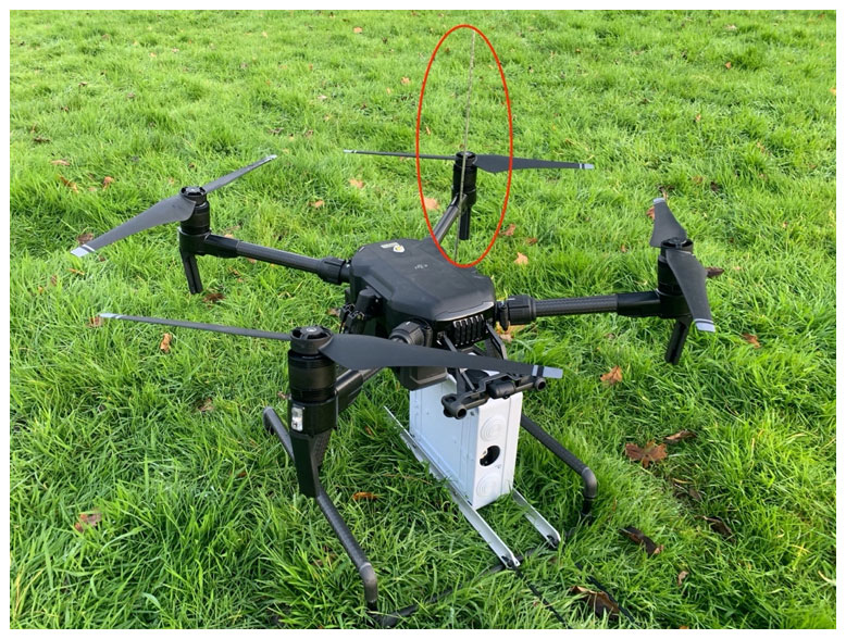
Figure 1The DJI Matrice 200 V2 with the POPS (white box at the left bottom of the fuselage). The red oval shows the inlet tube leading to the POPS.
Table 1Summary of the PNCs of each test flight at three stages. n/a = not applicable. The numbers denoted by ±x represent the standard deviation in the PNCs during the measurement time period. An asterisk (∗) indicates that profiles were also performed as documented here. T10: 5–60 m at 0.5 m s−1; T12: 5–70 m at 1.0 m s−1; T13: 2–90 m at 1.0 m s−1.
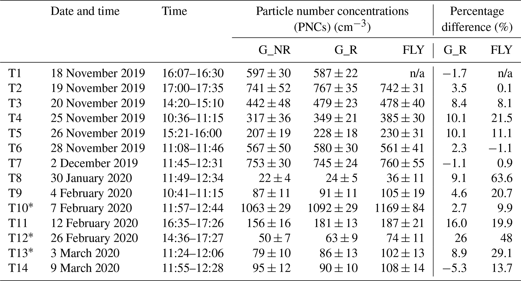
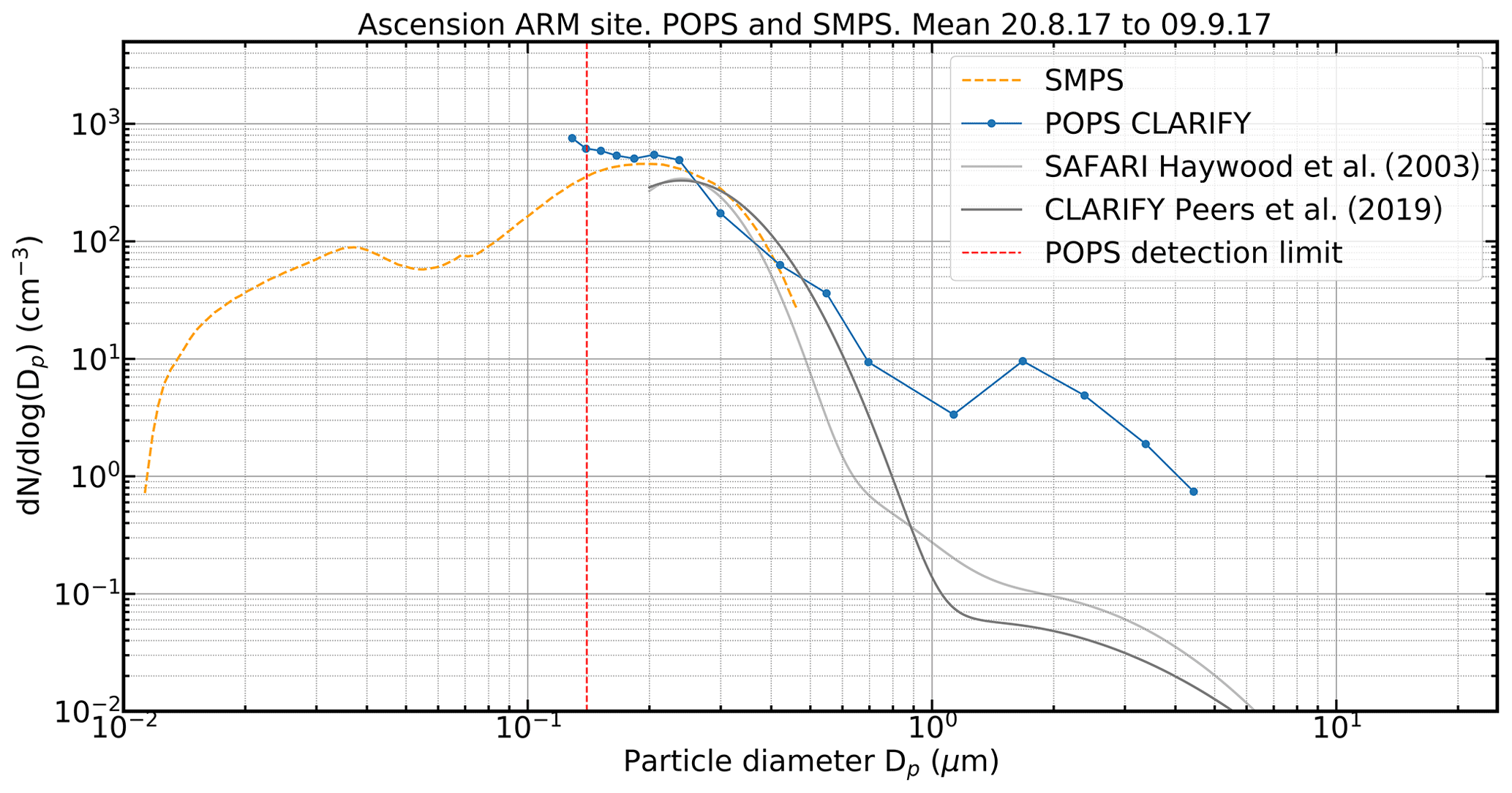
Figure 2PSDs from POPS, SMPS, and data fitted to a wing-mounted PCASP from CLARIFY-2017 and SAFARI-2000. POPS and SMPS data were collected at the ARM mobile site on Ascension Island from 20 August to 9 September 2017. The PCASP data from CLARIFY were collected from a flight on 4 September 2017 (Peers et al., 2019). The PCASP data from SAFARI-2000 represent a mean from 11 flights performed off the coast of Namibia (Haywood et al., 2003b). Note that the CLARIFY-210 and SAFARAI-2000 PCASP distributions are “scaled” to the SMPS size distribution to aid comparison. The POPS and SMPS values are not scaled.
3.1 Comparison of POPS data against data from LASIC/CLARIFY-2017
Figure 2 shows the mean PSD measured by the POPS and SMPS for the 20 d period, respectively. Figure 2 represents the whole size range of the two instruments as well as the fitted PSD from measurements with a wing-mounted PCASP-100X mounted on the UK's Bae146 FAAM aircraft from a flight during CLARIFY-2017 (Peers et al., 2019), which has been shown to be representative of biomass burning aerosol during the wider CLARIFY-2017 measurement campaign (Wu et al., 2020). The POPS and SMPS were sampling at around 330 m altitude a.s.l. when at the LASIC site, while the PCASP data from the CLARIFY campaign were collected from 1.9–7.3 km a.s.l. That the POPS and SMPS show close overlap at the peak concentrations indicates that the counting statistics and the particle concentrations are similar between the instruments. The mean PSD measured by the POPS and SMPS shows reasonable agreement. Although the agreement is not as good as that demonstrated in other comparisons against SMPS instruments (e.g. Gao et al., 2016), any resulting errors in derived optical parameters are likely to be small provided the fit is reasonable over the 0.2–1.0 µm diameter range. Measurements of biomass burning aerosol over the Atlantic from the SAFARI-2000 campaign suggest that particles in this range contribute 93 % of the scattering at 0.55 µm (e.g. Table 1, Haywood et al., 2003b). The PSD from the wing-borne PCASP-100X that was operated on the FAAM bears a close resemblance to the SMPS and POPS PSDs except at particle sizes < 0.2 µm diameter and > 0.7 µm diameter. The discrepancy at particle sizes < 0.2 µm might be expected because the fits that are adopted by Haywood et al. (2003a) and Peers et al. (2019) do not account for these small particles as they were developed with simplicity in mind for global general circulation models and for satellite retrievals, respectively. Aerosols > 0.7 µm diameter that were observed by the POPS that were not present in the CLARIFY-2017 or SAFARI-2000 data may well be generated by dust generation from the arid surface of Ascension Island or by super-micron sea salt from breaking waves. Taylor et al. (2020) document the enhanced influence of the oceanic component of aerosols in the marine boundary layer, but this is not included in the CLARIFY-2017 or SAFARI-2000 log-normal fits, which represent biomass burning aerosols only. Thus, the POPS instrument appears to provide a reasonably quantitative measure of optically active sub-micron biomass burning aerosols.
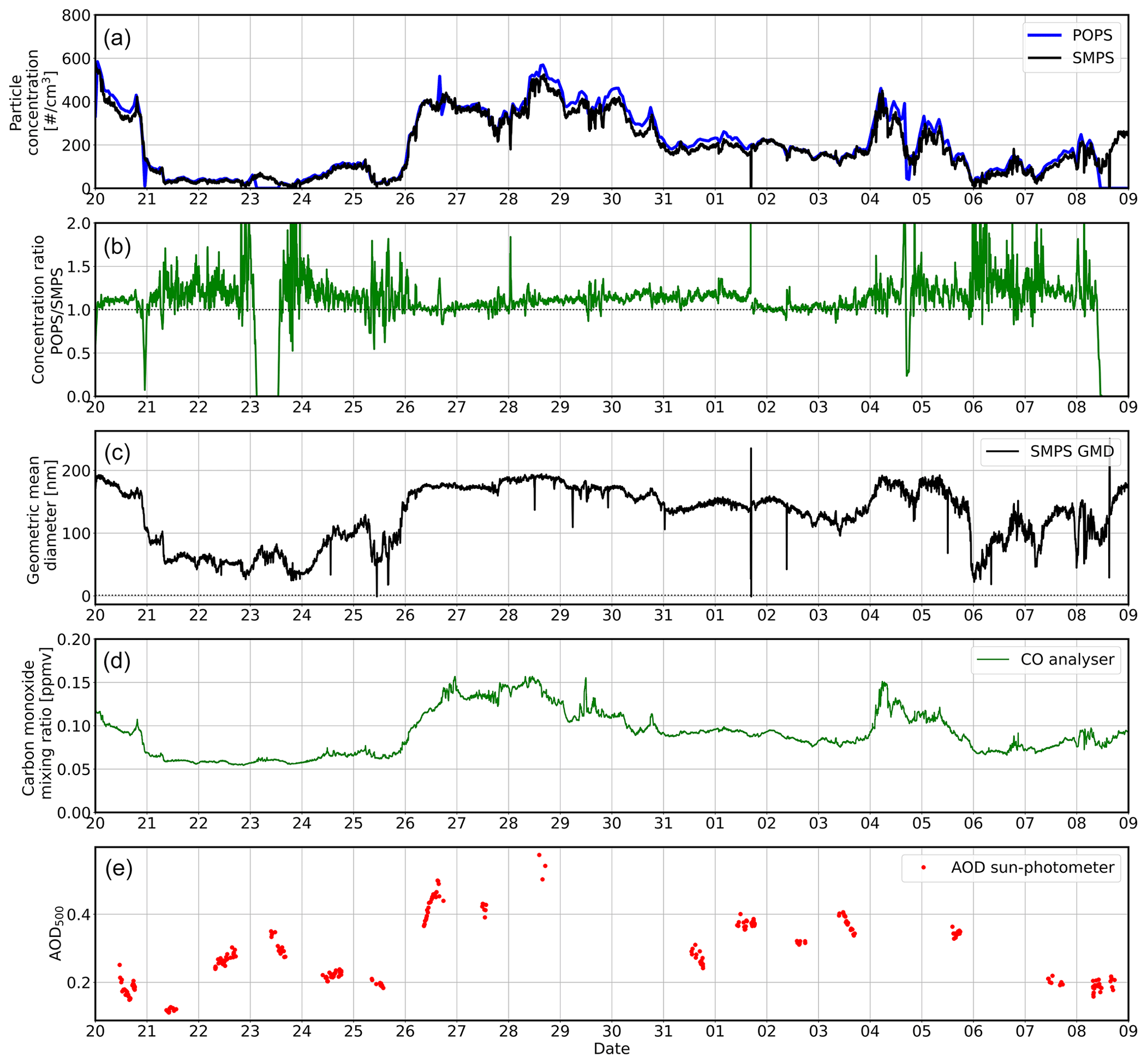
Figure 3(a) Time series of SMPS and POPS particle concentrations in the diameter range 120–450 nm measured during the LASIC/CLARIFY-2017 campaign. (b) Ratio of the POPS to SMPS concentrations shown in (a). (c) Geometric mean diameter from SMPS. (d) Carbon monoxide mixing ratio from Los Gatos Research CO analyser, and (e) AOD from Cimel sun-photometer.
We also investigated the overall particle number concentration from the POPS and examine the time series of the POPS measurements against some other key variables measured by the SMPS and other instrumentation at the ARM mobile facility. Figure 3a presents the 20 d intercomparison of the PNCs from the POPS and SMPS, and 3b shows the ratio of the two concentration measurements (POPS/SMPS). They show a good agreement between two instruments, while the geometric mean diameter (GMD) of the size distribution (Fig. 3c) is above 0.12 µm. Again, this illustrates that the POPS instrument measures accumulation mode aerosols reasonably accurately.
We would expect biomass burning aerosols to be associated with an increase in carbon monoxide (CO; Haywood et al., 2003b; Wu et al., 2020), and the concentrations measured by both the POPS and SMPS instruments are well correlated with the CO volume mixing ratio (as measured by a co-located CO analyser – Fig. 3d). The concentration data also show some correlation with the AODs as measured by a co-located AERONET Cimel sun photometer (Fig. 3e), although this AOD is a column measurement rather than a point measurement so the influence of vertical profile will likely be important (e.g. Wu et al., 2020; Haywood et al., 2021).
3.2 Test flight results
To determine the impact of rotors and drone attitude on the POPS, we focus on the comparison of PSD and PNC at three different stages: G_NR, G_R, and FLY. Table 1 summarizes the mean PNC with standard deviation and the PNC percentage differences of each flight at different stages.
3.2.1 Particle number concentration (PNC)
Compared with the mean PNC at G_NR, the mean PNC at G_R changed from −1 % to 26 %, and that at FLY changed from −1 % to 63 %, respectively. However, it is apparent that the differences of PNCs are much lower in the cases T1, T2, T6, T7, and T10 (less than 10 %) in both stages. Figure 4 shows the probability density functions of PNC in each case. A constant bin width is utilized across the G_NR, G_R, and FLY PDFs of each flight. Unpaired two-sample t tests were selected to detect the similarity of the PNCs at different stages as the t test is the most popular parametric test for samples following normal distribution for calculating the significance of a small sample size (De Winter, 2013). Here the PNC of G_NR was set as the control group, while that of G_R and FLY was set as the perturbation groups using the mean PNC at each stage every 30 s. Before the t test, Levene's test was performed, which is an inferential statistic used to assess the equality of variances for a variable calculated for two or more groups (Burkholder, 1962). If Levene's test cannot be passed, then the unequal variances t test, which is a more conservative test, was be applied for the groups. The results (p value) of the t test of each test flight are shown in Table 2.
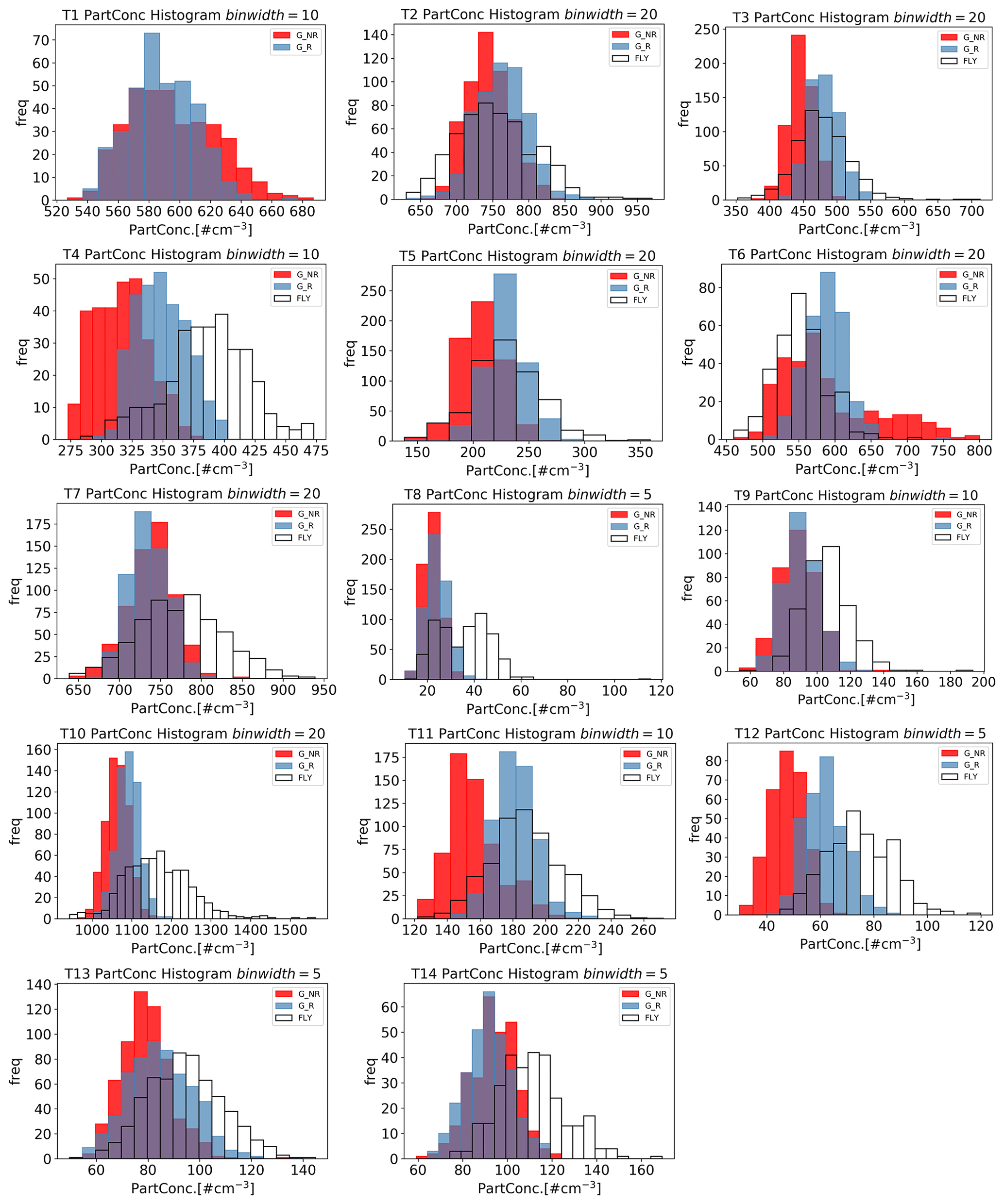
Figure 4Probability density functions (PDFs) of PNCs in each case. A constant bin width is utilized across the G_NR, G_R, and FLY PDFs of each flight.
Table 2Summary of the dates, time, wind speed, and t test results (p value) of each test flight. Wind speed values (at 1.5 m) are the wind speed in the hour closest to the experiment time. From T10 to T14 the wind speed data are not available (NA) because the instrument recording the data had broken. Flights highlighted in bold font indicate that the results are not significantly different at 5 % significance. Flights marked in italic font indicate that the PNC on the ground with the rotor on are not significantly different from G_NR, and flights marked in standard font indicate that there are significant differences in both G_R and FLY when compared to G_NR.

For a significance level (α) set as 0.05, there are five test flights that passed the t test in both G_R and FLY stages (p value ≥ α), which means the PNC measured at G_R and FLY stage corresponded well with those measured at G_NR. These test numbers have been marked in bold italic font in Table 2. This result indicates that the impact of rotors and UAV attitude was not significant in these five cases. The other three cases (T8, T9, and T14) passed the t test in the G_R stage, which are marked in italic font. The rest of test flights did not pass the t test in either stage (marked in standard font). Through comparing the weather conditions, we find that the wind speed (Table 2) was relatively lower (0.5–2.6 m s−1) in the cases which pass the t test at both stages. The wind speed in Table 2 was provided from observations at Exeter airport with 1 h resolution. During the actual experiment, when the wind speed was high, visual observations by the drone pilot suggested that the drone swung from side to side in the air, causing increased variability in the pitch, yaw, and altitude of the drone. As previously noted, on T9 and T13 the drone was forced to land early to ensure safety due to the high (> 7 m s−1) instantaneous wind speed.
To determine the impact of wind speed on PNC observed by the POPS, the cases are separated into two categories: low wind speed (w < 2.6 m s−1) cases and high wind speed (2.6 < w < 7.7 m s−1) cases. The PNC root mean square differences (RMSD) and mean absolute differences (MAD) at G_R and FLY for all cases, low wind speed cases, and high wind speed cases are given in Table 3. For all cases, PNC RMSD is less than 10.2 % at G_R and less than 26.2 % at FLY, and MAD is less than 7.8 % at G_R and less than 19.1 % at FLY. However, in the low wind cases, the RMSD and MAD fall to 2.4 % and 2.3 % at G_R, and 5 % and 3 % at FLY, respectively. In contrast, RMSD and MAD in the high wind cases increase to 12.6 % and 10.9 % at G_R and to 31.4 % and 26.3 % at FLY, respectively. The variability in the pitch, yaw, and altitude of the drone also impacted the orientation of the inlet of the POPS, which ideally should be perpendicular to the horizontal plane. Variations in the orientation of the inlet led to increased scatter in the sample flow rate. Table 4 shows mean sample flow rates with standard deviation at G_NR, G_R, and FLY for all cases. It is clear that for G_NR, the mean flow rates were constant across all tests and the standard deviation in the flow rates were very low. Comparing with G_NR, the mean sample flow rate and the standard deviation were almost unchanged for G_R. This shows that operating the rotors alone did not impact the sample flow rate. However, while the mean flow rate during FLY was identical to G_NR, the standard deviations increased during the FLY stage, particularly for the tests under high wind speeds. The mean value of the standard deviation for low wind speed cases was 0.13, while for the high wind speed cases it was 0.21, which may influence the accuracy of the POPS measurements.
Table 3Summary of RMSD and MAD for all cases, low wind cases, and high wind cases.
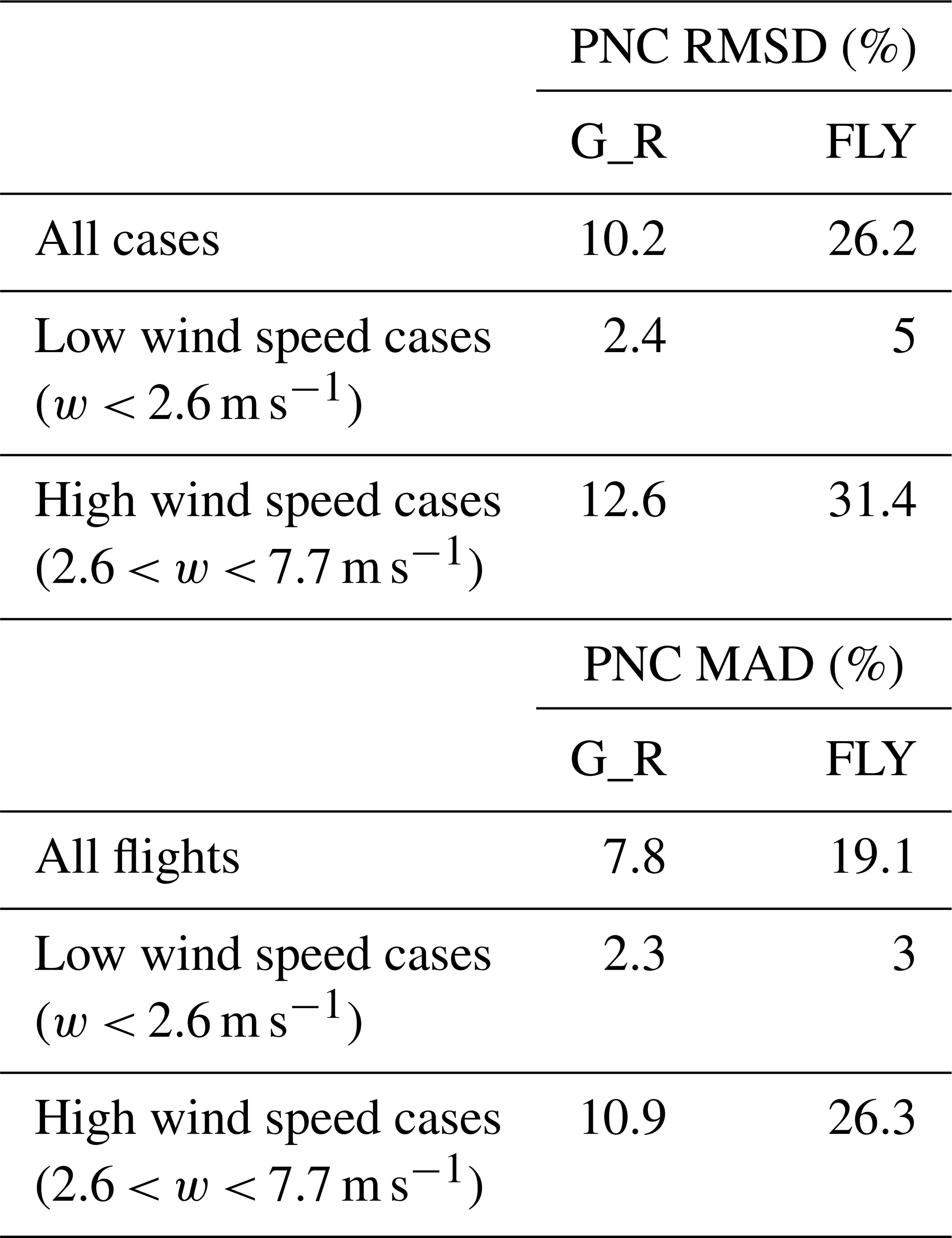
Table 4Summary of the sample flow rates of each test flight at three stages. n/a = not applicable. The numbers denoted by ±x represent the standard deviation in the sample flow rates during the measurement time period.

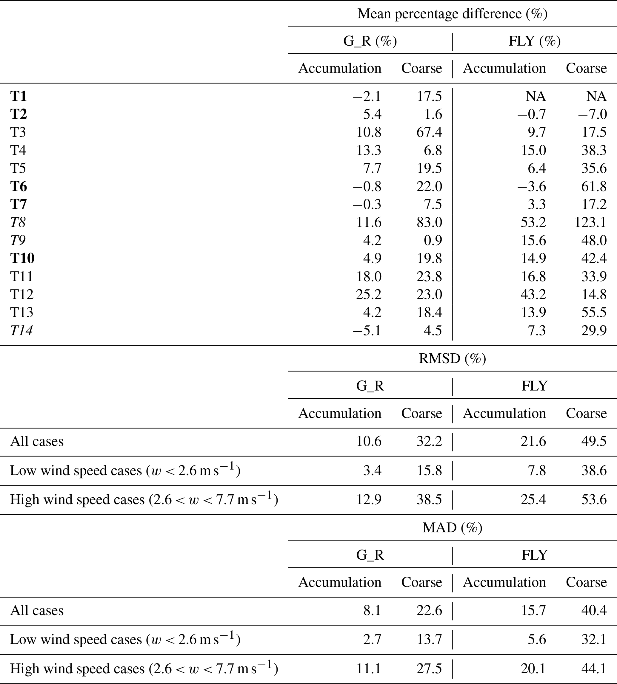
Table 5Summary of mean percentage differences of size distribution between G_NR and G_R and between G_NR and FLY of each flight. The size distributions are separated into two modes: accumulation mode (0.1 ≤ d ≤ 1 µm) and coarse mode (d > 1 µm).
3.2.2 The particle size distribution (PSD)
The PSDs at different stages and the mean PSD ratios at G_R to G_NR and FLY to G_NR of each test flight are shown in Fig. 5, which indicates that the cases with high similarity of PNCs (T1, T2, T6, T7, and T10) show agreement of the PSD. It also shows that the differences in sub-micron sizes are less than those in super-micron sizes at G_R and FLY. Therefore, the size distribution was separated into two modes, the accumulation mode (0.1 ≤ d ≤ 1.0 µm) and the coarse mode (d > 1.0 µm), to make a statistical analysis. Table 5 summarizes the PSDs percentage differences for two modes at G_R and FLY for each case. The PSDs RMSD and MAD for two modes at G_R and FLY for all cases, low wind cases, and high wind cases are given in Table 5. The percentage differences of the PSDs are less than 5.4 % and 14.9 % in low wind cases at the accumulation mode at G_R and FLY, respectively, while the variation in the PSD in the coarse mode is perhaps due to lower counting statistics at these sizes. In contrast PSDs of other cases show differences across the whole spectrum. Even in the accumulation mode, the differences of the PSDs between FLY and G_NR are up to 53.2 % in the case T8. PSDs RMSD and MAD at the accumulation mode are 3.4 % and 2.7 % respectively at G_R in the low wind speed cases, but up to 12.9 % and 11.1 % at G_R in the high wind speed cases. These statistics again indicate that impacts of rotors and UAV attitude on the POPS measurements appear to be reduced in low wind speeds relative to higher wind speeds. PSD RMSDs and MADs at the coarse mode at G_R and at the accumulation and coarse mode at FLY show the same result. Generally speaking, RMSDs and MADs indicate the impact of rotors and UAV attitude on the performance of the POPS in measuring the accumulation mode is lower than in measuring the coarse mode, for all cases. RMSDs in accumulation mode were 10.6 % at G_R and 21.6 % at FLY, while those in coarse mode were 32.2 % and 49.5 % for all cases. MADs showed the same trend as RMSDs. In the absence of independent multi-stage meteorological tower measurements (e.g. Ahn, 2019), it is difficult to assess how much of the variability in PNCs and PSDs is real, particularly when the drone is flying; there may be changes in PNC with altitude when compared to the surface PNCs owing to surface deposition. Alternatively, there may be trends in the particle concentrations that occur during the entire measurement period, which spanned around 30 min duration. We determine trends in the G_NR and G_R statistics by determining the mean slope (particles s−1) during the operating periods; only flights T4 and T6 show trends of greater than 0.1 particles s−1 (6 particles min−1) when averaged over both G_NR and G_R. Figure 4 shows that there is potentially an increase in the concentrations that are measured during T4, and that there is potentially a bi-modal number concentration measured during the G_NR sampling period for T6. As no trends are evident for the other flights, it can be inferred that there is no evidence of a significant systematic trend in atmospheric concentrations across all flights; any such trends are likely to be random. However, a potential solution to any concern would be to change the three-stage sequence from G_NR, G_R, and FLY to a five stage sequence of G_NR, G_R, FLY, G_R, and G_NR. This sequence is suggested for future investigations.

Figure 5Particle size distribution at three stages: the drone on the ground with rotors off (G_NR) (red line), on the ground with rotors on (G_R) (blue line), and flying at 10 m (FLY) (grey line), in each POPS test. The ratios of the PSD at G_R to G_NR (blue dash line) and at FLY to G_NR (grey dash line) of each flight are given in each plot.
3.2.3 The PNC during vertical profiles
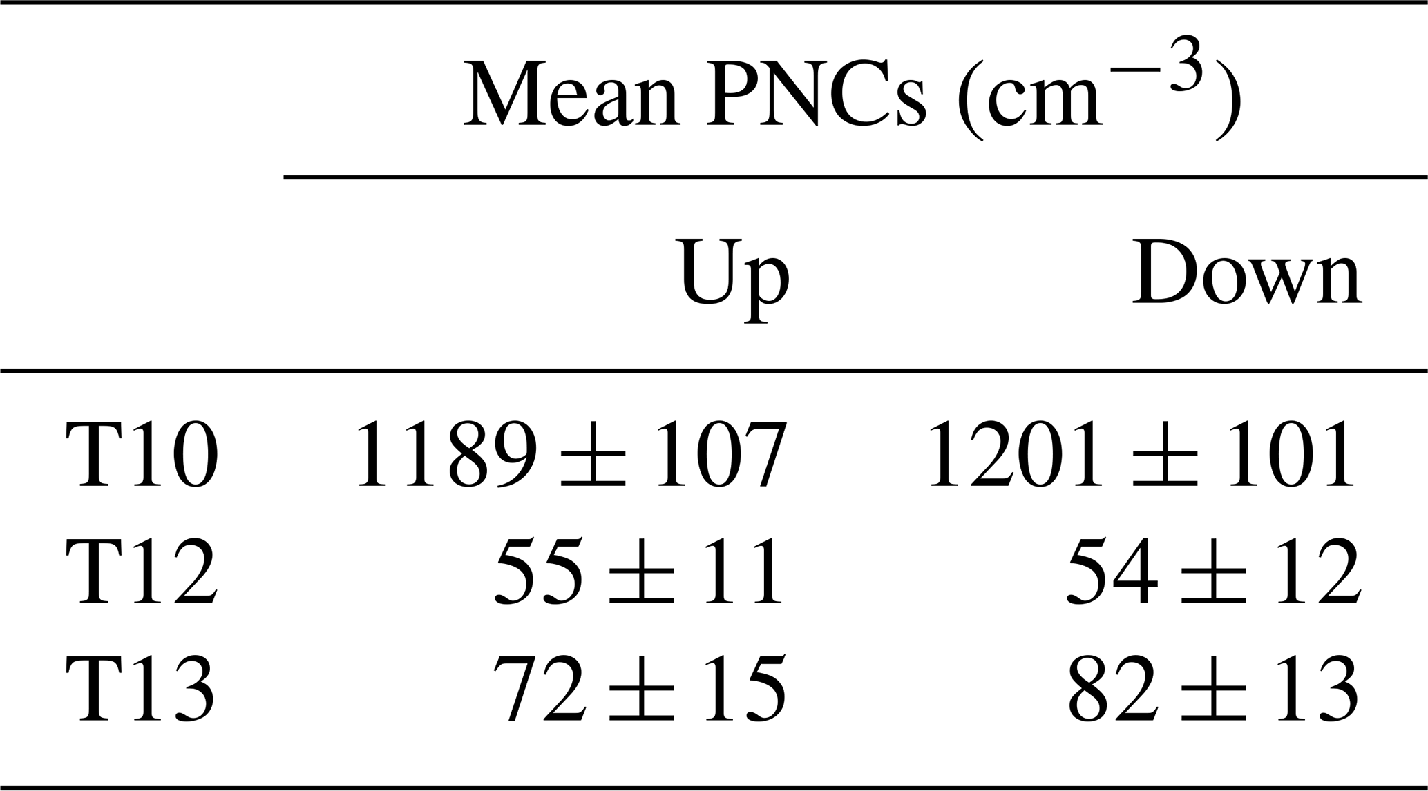
Figure 6 presents the results of the vertical profile runs in T10, T12, and T13. The mean PNCs with standard deviation on the way up and down are shown in Table 6. The PNCs measured on the way up and way down show agreement. The best agreement is found in the high number concentration, low wind speed case (T10), where the PNCs differ by an average of 0.5 % between ascent and descent. Even in the high wind speed cases when the variability might be expected to be largest owing to changes in the pitch and yaw of the drone, general agreement is found indicating that the vertical speed of the drone (which was approximately 0.5 to 1 m s−1) does not appear to have a significant impact. Note that the vertical profiles do indicate some variability in the vertical distribution with PNCs ranging from 1207 ± 83, 69 ± 14, and 90 ± 11 cm−3 close to the surface to 1189 ± 107, 55 ± 11, and 72 ± 15 cm−3 in ascent and 1395 ± 83, 69 ± 5, and 89 ± 6 cm−3 close to the surface to 1201 ± 101, 54 ± 12, and 82 ± 13 cm−3 in descent for flights T10, T12, and T13. The close-to-surface data were collected by the UAV-mounted POPS when the drone was 1–3 m above the surface. This variability with height emphasizes the utility of small, instrumented UAVs for measuring PNCs and PSDs at low altitudes; measurements at such altitudes are impossible to probe with heavily equipped atmospheric research aircraft operating under standard aviation safety protocols.
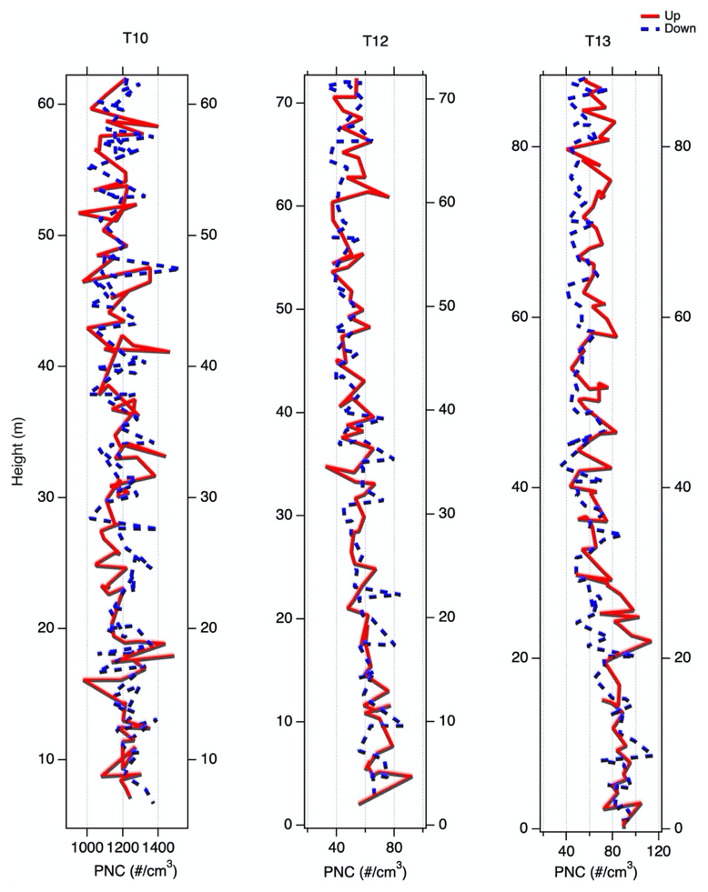
Figure 6Vertical profiles of the particle number concentration in the profile runs of T10, T12, and T13. The red line shows the observed concentration on the way up and the blue dash line shows that on the way down, respectively.
Table 6Mean PNC with standard deviations on the way up and down in three vertical profile runs.
We have investigated the performance of POPS against a reference SMPS instrument while on the ground and also while operated on a quadcopter drone, DJI Matrice 200 V2, which is the first documented test of the performance of a POPS instrument on a UAV. The investigation includes two parts. The first is a long-term comparison between the POPS and other instruments during the CLARIFY-2017/LASIC and SAFARI-2000 project. The results show that the PNC measured by the POPS and that measured by the SMPS and PCASP indicate agreement in the optically important size range centred at around 0.3 µm diameter. This indicates that despite its small size, when operating under controlled conditions on the ground, the POPS instrument performs relatively well. In the second part, we tested the impact of drone's rotors, and indirectly the attitude of the drone, on the performance of the POPS with a focus on two aspects, the PNC and PSD. We found RMSDs and MADs in PNC when operating a POPS on a small quadcopter to be less than 10.2 % and 7.8 %, respectively, when operating on the ground, and less than 26.2 % and 19.1 %, respectively, at 10 m altitude under wind speed conditions of up to 7.7 m s−1. For wind speed of less than 2.6 m s−1, RMSDs and MADs fell to 2.4 % and 2.3 % when operating on the ground, and to 5 % and 3 % at 10 m altitude. We also found no statistical difference in PNC when operating the UAV in either ascent or descent. As for the PSD, the accumulation mode aerosol size distributions were relatively invariant between measurements at the surface and measurements at 10 m altitude with RMSD and MAD of less than 21.6 % and 15.7 %, respectively. The differences between coarse mode super-micron aerosols measured at the surface and at 10 m altitude were universally greater than those measured at the surface with a RMSD and MAD approaching 49.5 % and 40.4 %, but it is unclear whether this is due to loss of coarse mode aerosol particles to the surface or whether this is due to interference from the rotors. This impact appears to be most prevalent at the larger end of the POPS size range. While the increase in PNC from G_NR to G_R might be explained by generation or resuspension of aerosols from the surface by the rotors of the UAV, the increase from G_R to FLY is more difficult to attribute. The surface acts as a net sink in aerosols through dry deposition which could lead to an increase in PNC with altitude (e.g. Pellerin et al., 2017), but there are confounding factors from changes in the attitude of the drone and rapid changes in the attitude necessary for stabilizing the position of the UAV during FLY that could also influence the measurements. Indeed, there is evidence that fast adjustments to the attitude of the UAV increase the variability in the flow rate reported by the POPS sensor, particularly at higher wind speeds, where these corrections are larger. These results suggest that, when the wind speed is modest, the POPS and UAV and very simple inlet combination examined here appear able to measure the aerosol PSD and PNC with reasonable fidelity, particularly for sub-micron aerosols.
In follow-up scientific observations, the POPS deployed on the quadcopter drone will be used to measure the aerosol properties in the atmospheric boundary layer (ABL) under polluted conditions. Concentrations of pollutants in the ABL frequently have a strong correlation with atmospheric stability (Wang et al., 2013; Chambers et al., 2015) with stable conditions leading to the build-up of pollutants in the ABL. Wind speeds are frequently low in stable conditions due to the lack of convection-driven turbulence. Because these future measurements are likely under stable, non-turbulent conditions, wind speed effects are not likely to cause significant problems. For other applications of the POPS on a quadcopter drone, such as the dispersion of pollutants in down-wind driven plumes, attention should be paid to the influence of the higher wind speeds.
A1 POPS calibration
The calibration procedure used to adjust the POPS size bins for refractive index followed the general OPC calibration methodology described in Rosenberg et al. (2012) and Gao et al. (2016). By sampling a series of mono-disperse particles of known refractive index we compared the scattering amplitudes measured by the POPS to scattering amplitudes calculated using Mie theory. Scaling the Mie-calculated amplitudes to match the measured scattering amplitudes results in a scaling factor that accounts for the POPS laser energy and detector efficiency. The scaling factor can then be used to convert Mie-calculated scattering amplitudes for any refractive index to the arbitrary units of the POPS.
A2 Calibration measurements
The calibration used NIST traceable polystyrene latex (PSL) spheres in 22 sizes, ranging from 0.147 to 3 µm. The manufacturer's stated refractive index is 1.615−0.001i. An air source and a nebulizer cup were connected via rubber tubing to the POPS inlet and a few minutes of data collected for each of the 22 sizes of PSL sphere. The result was a histogram of POPS digitizer values for each size. We fitted normal distributions to these and took the mode and standard deviation as the POPS scattering value and associated error.
A3 Polarized Mie scattering calculations for the POPS geometry
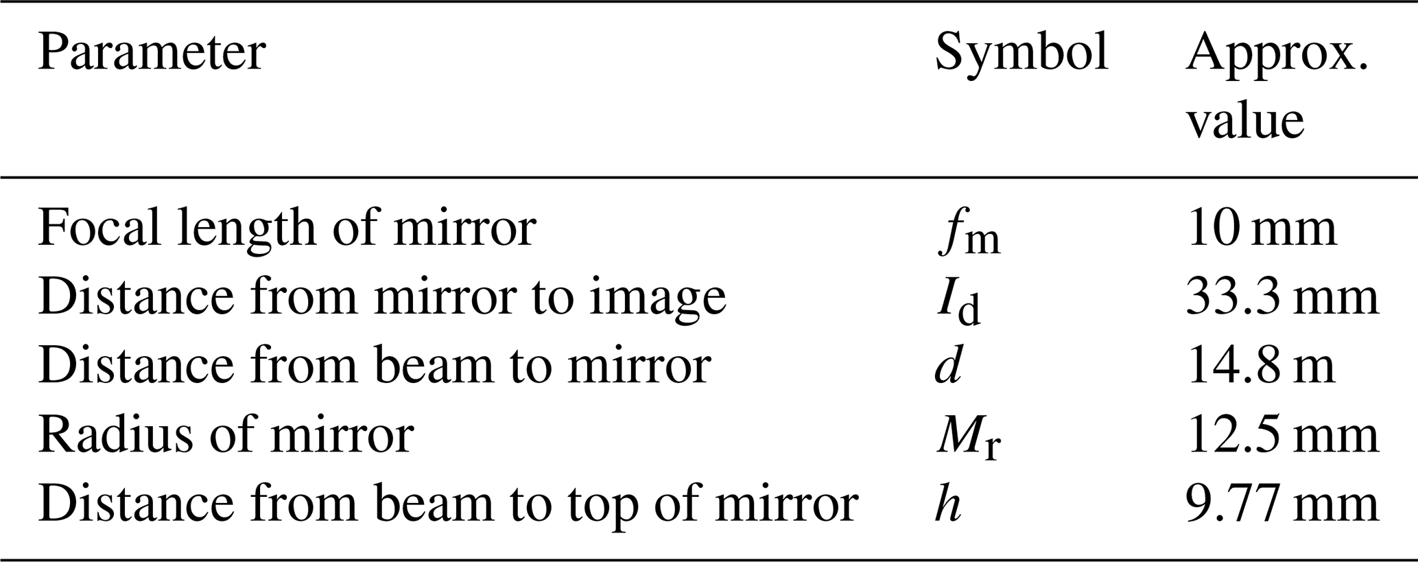
The Mie scattering calculations were made using the miepython library available from https://pypi.org/project/miepython/ (last access: 12 March 2021). We calculated POPS specific scattering amplitudes for spherical particles by integrating the scattering phase functions over only the POPS collection angles. Gao et al. (2016) describes the geometry of the POPS detection chamber and this is shown in Fig. A1.
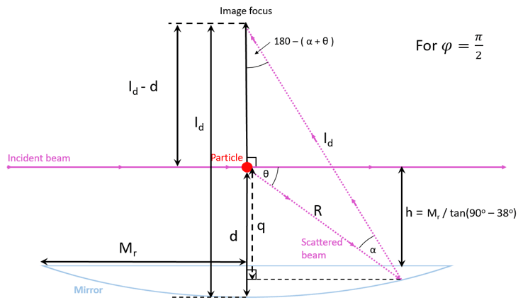
Figure A1Geometry of POPS optical chamber. Values for the fixed parameters are listed in Table A1.
According to Bohren and Huffman (2008), for a homogeneous spherical particle illuminated by an electromagnetic plane wave , the scattered wave as observed a constant distance from the particle can be written as
where are the components of the electric fields parallel and perpendicular to the scattering plane, and S1 and S2 are elements of the amplitude scattering matrix describing the angular distribution of the scattered light. According to Gao et al. (2016) the POPS laser diode is oriented such that the plane of polarization of the laser is perpendicular to the scattering plane (so perpendicular to the plane of the page in Fig. 1), and so zero. As the diagonal elements of the amplitude scattering matrix are zero, E∥s is also zero, meaning that the scattered field contains no component parallel to the scattering plane. Therefore, the scattering amplitude for the POPS, σpops, is given by
where θ and φ are the zenith and azimuthal scattering angles respectively (we measure φ from horizontal – that is downwards from the plane perpendicular to the page in Fig. A1). Dp is particle diameter, Qsca is the Mie scattering efficiency factor, and Fpops is a weighting function that accounts for the collection angles of the POPS. To construct the weighting function Fpops we find the combinations of θ and φ for which the phase function hits the collection mirror (Fpops=1) and when it is outside of the mirror (Fpops=0). From Fig. A1 and the information given in Table A1, for and , the scattered beam hits the collection mirror a vertical distance q from the axis of the incident beam given by
where
and
and using the lens equation
For a given value of θ, as the azimuthal angle φ rotates away from , the distance q will shorten by a factor of cos (90−φ), and when q is less than the distance h (the distance from the beam to the horizon of the mirror) the scattered beam will no longer hit the mirror. So finally, for we have
Table A1Parameters derived from information in Gao et al. (2016).
A4 Results
The blue curve in Fig. A2 is the result of using Eqs. (A1) and (A7) and a refractive index of 1.615−0.001i for particle diameters 0.1 to 4 µm (as a sanity check, this curve is nearly identical in shape to that shown in Fig. 6 of Gao et al., 2016). The scattering amplitudes measured during the calibration using PSL spheres are plotted in red. The vertical error bars are 1 standard deviation of the normal distribution. The Mie scattering curve has been scaled (using a least squares fit) to match the scattering amplitudes measured during the calibration.
The black curve in Fig. A2 is the result of using a biomass-burning-like refractive index of 1.54−0.27i in the Mie calculations. This curve has also been scaled using the same factor as the blue PSL sphere curve.
A5 Bin boundaries for biomass-burning-like particles
For particle sizing, we used 16 bins logarithmically spaced along the scattering amplitude axis. We then used a monotonic fit to the scaled scattering amplitude curve for biomass burning to relate these bin boundaries to particle diameters, giving the bin boundaries as shown in Fig. A3.
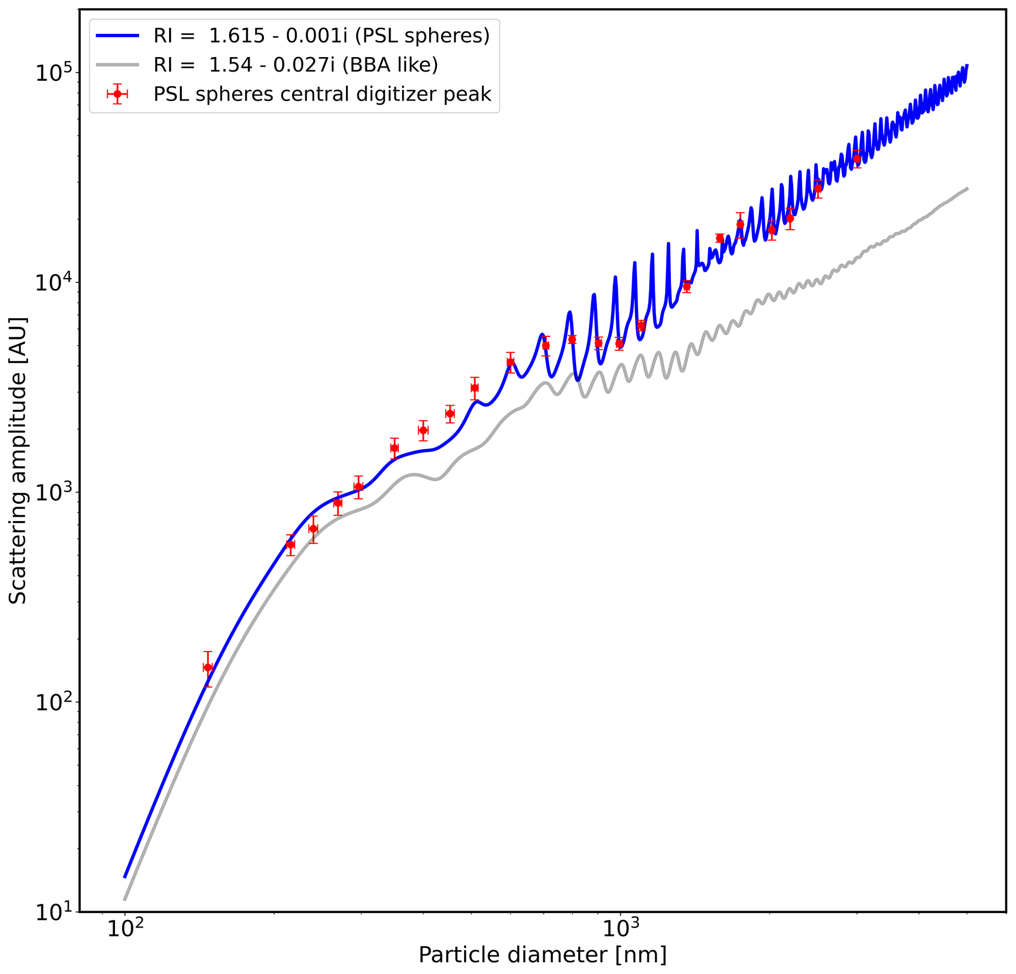
Figure A2POPS scattering amplitudes for particles from 0.1 to 4 µm. Calculations for the blue curve used the refractive index for PSL spheres and for the black curve a refractive index for biomass burning particles. The red points are the real scattering amplitudes measured during the calibration with PSL spheres. Both the blue and black curves have been scaled using the same scaling factor.
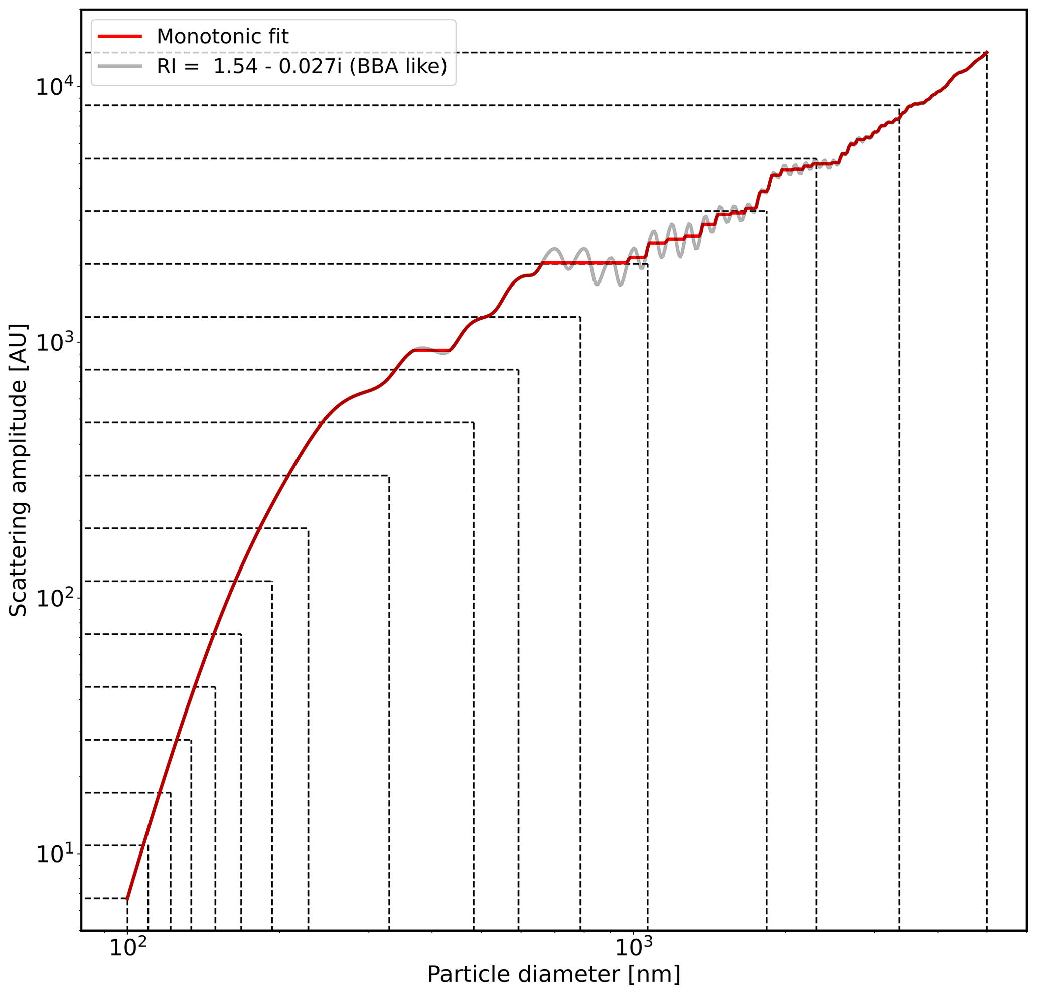
Figure A316 bin boundaries logarithmically spaced in terms of peak value related to particle diameter using the scaled biomass burning curve from Fig. A2. The red line is a monotonically increasing fit.
Code used in this study can be obtained upon reasonable request from Zixia Liu (zixia.liu@kcl.ac.uk).
The data presented in this study can be provided upon reasonable request from Zixia Liu (zixia.liu@kcl.ac.uk).
The study was completed with close cooperation between all authors. ZL, MO, and JH conceived the idea for this article; ZL, MO, JH, and AW designed and produced the experimental platform; ZL and MO conducted the data analyses; ZL and JH discussed the experimental results; ZL wrote the manuscript; ZL, MO, and JH modified the manuscript; and all co-authors helped review the manuscript.
The authors declare that they have no conflict of interest.
Publisher’s note: Copernicus Publications remains neutral with regard to jurisdictional claims in published maps and institutional affiliations.
This work was supported by the Chinese University of Hong Kong–University of Exeter Joint Centre for ENvironmental SUstainability and REsilience (ENSURE) programme; Zixia Liu, Martin Osborne, James Haywood, Karen Anderson, Jamie D. Shutler, Tao Huang, Jack C. H. Cheng, and Steve H. L. Yim would like to thank ENSURE for their financial support. James Haywood, Zixia Liu, and Hugh Coe would also like to acknowledge NERC SWAAMI (South West Asian Aerosol Monsoon Interactions) for partial funding of the research.
This research has been supported by the Natural Environment Research Council (NERC) SWAAMI (grant no. NE/L013886/1) and CLARIFY-2017 Large Grant (grant no. NE/L013584/1), the University of Exeter (grant no. NE/L013878/1), and the Chinese University of Hong Kong (grant no. NE/L013878/1).
This paper was edited by Troy Thornberry and reviewed by two anonymous referees.
Ahn, K.-H.: Aerosol 3D Profiling Using Compact Particle Measuring Instruments with Balloon and Drone System, in: 7th International Symposium on Ultrafine Particles, Air Quality and Climate, 15–16 May 2019, Brüssel, Belgium, 2019.
Atkinson, D. B., Radney, J. G., Lum, J., Kolesar, K. R., Cziczo, D. J., Pekour, M. S., Zhang, Q., Setyan, A., Zelenyuk, A., and Cappa, C. D.: Aerosol optical hygroscopicity measurements during the 2010 CARES campaign, Atmos. Chem. Phys., 15, 4045–4061, https://doi.org/10.5194/acp-15-4045-2015, 2015.
Atkinson, D. B., Pekour, M., Chand, D., Radney, J. G., Kolesar, K. R., Zhang, Q., Setyan, A., O'Neill, N. T., and Cappa, C. D.: Using spectral methods to obtain particle size information from optical data: applications to measurements from CARES 2010, Atmos. Chem. Phys., 18, 5499–5514, https://doi.org/10.5194/acp-18-5499-2018, 2018.
Bellouin, N., Boucher, O., Haywood, J., and Reddy, M. S.: Global estimate of aerosol direct radiative forcing from satellite measurements, Nature, 438, 1138–1141, 2005.
Bezantakos, S., Schmidt-Ott, F., and Biskos, G.: Performance evaluation of the cost-effective and lightweight Alphasense optical particle counter for use onboard unmanned aerial vehicles, Aerosol Sci. Technol., 52, 385–392, 2018.
Bohren, C. F. and Huffman, D. R.: Absorption and scattering of light by small particles, John Wiley & Sons, New York, 2008.
Boucher, O., Randall, D., Artaxo, P., Bretherton, C., Feingold, G., Forster, P., Kerminen, V.-M., Kondo, Y., Liao, H., Lohmann, U., Rasch, P., Satheesh, S. K., Sherwood, S., Stevens, B., and Zhang, X. Y.: Clouds and Aerosols, in: Climate Change 2013: The Physical Science Basis, Contribution of Working Group I to the Fifth Assessment Report of the Intergovernmental Panel on Climate Change, edited by: Stocker, T. F., Qin, D., Plattner, G.-K., Tignor, M., Allen, S. K., Boschung, J., Nauels, A., Xia, Y., Bex, V., and Midgley, P. M., Cambridge University Press, Cambridge, United Kingdom and New York, NY, USA, available at: http://www.climatechange2013.org/images/uploads/WGIAR5_WGI-12Doc2b_FinalDraft_Chapter07.pdf (last access: 15 January 2021), 2013.
Burkart, J., Steiner, G., Reischl, G., Moshammer, H., Neuberger, M., and Hitzenberger, R.: Characterizing the performance of two optical particle counters (Grimm OPC1. 108 and OPC1. 109) under urban aerosol conditions, J. Aerosol Sci., 41, 953–962, 2010.
Burkholder, D. L.: Contributions to Probability and Statistics: Essays in Honor of Harold Hotelling., J. Am. Stat. Assoc., 57, 205–207, https://doi.org/10.2307/2282455, 1962.
Chambers, S. D., Wang, F., Williams, A. G., Xiaodong, D., Zhang, H., Lonati, G., Crawford, J., Griffiths, A. D., Ianniello, A., and Allegrini, I.: Quantifying the influences of atmospheric stability on air pollution in Lanzhou, China, using a radon-based stability monitor, Atmos. Environ., 107, 233–243, 2015.
De Winter, J. C. F.: Using the Student's t-test with extremely small sample sizes, Pract. Assess. Res. Eval., 18, 10, https://doi.org/10.7275/e4r6-dj05, 2013.
Gao, R. S., Perring, A. E., Thornberry, T. D., Rollins, A. W., Schwarz, J. P., Ciciora, S. J., and Fahey, D. W.: A high-sensitivity low-cost optical particle counter design, Aerosol Sci. Technol., 47, 137–145, 2013.
Gao, R. S., Telg, H., McLaughlin, R. J., Ciciora, S. J., Watts, L. A., Richardson, M. S., Schwarz, J. P., Perring, A. E., Thornberry, T. D., and Rollins, A. W.: A light-weight, high-sensitivity particle spectrometer for PM2.5 aerosol measurements, Aerosol Sci. Technol., 50, 88–99, 2016.
Gu, Y. and Yim, S. H. L.: The air quality and health impacts of domestic trans-boundary pollution in various regions of China, Environ. Int., 97, 117–124, https://doi.org/10.1016/j.envint.2016.08.004, 2016.
Gu, Y., Wong, T. W., Law, C. K., Dong, G. H., Ho, K. F., Yang, Y., and Yim, S. H. L.: Impacts of sectoral emissions in China and the implications: air quality, public health, crop production, and economic costs, Environ. Res. Lett., 13, 084008, https://doi.org/10.1088/1748-9326/aad138, 2018.
Gu, Y., Zhang, W., Yang, Y., Wang, C., Streets, D. G., and Yim, S. H. L.: Assessing outdoor air quality and public health impact attributable to residential black carbon emissions in rural China, Resour. Conserv. Recycl., 159, 104812, https://doi.org/10.1016/j.resconrec.2020.104812, 2020.
Haywood, J. and Boucher, O.: Estimates of the direct and indirect radiative forcing due to tropospheric aerosols: A review, Rev. Geophys., 38, 513–543, 2000.
Haywood, J. M., Francis, P., Dubovik, O., Glew, M., and Holben, B.: Comparison of aerosol size distributions, radiative properties, and optical depths determined by aircraft observations and Sun photometers during SAFARI 2000, J. Geophys. Res., 108, 8471, https://doi.org/10.1029/2002JD002250, 2003a.
Haywood, J. M., Osborne, S. R., Francis, P. N., Keil, A., Formenti, P., Andreae, M. O., and Kaye, P. H.: The mean physical and optical properties of regional haze dominated by biomass burning aerosol measured from the C-130 aircraft during SAFARI 2000, J. Geophys. Res., 108, 8473, https://doi.org/10.1029/2002JD002226, 2003b.
Haywood, J. M., Abel, S. J., Barrett, P. A., Bellouin, N., Blyth, A., Bower, K. N., Brooks, M., Carslaw, K., Che, H., Coe, H., Cotterell, M. I., Crawford, I., Cui, Z., Davies, N., Dingley, B., Field, P., Formenti, P., Gordon, H., de Graaf, M., Herbert, R., Johnson, B., Jones, A. C., Langridge, J. M., Malavelle, F., Partridge, D. G., Peers, F., Redemann, J., Stier, P., Szpek, K., Taylor, J. W., Watson-Parris, D., Wood, R., Wu, H., and Zuidema, P.: The CLoud–Aerosol–Radiation Interaction and Forcing: Year 2017 (CLARIFY-2017) measurement campaign, Atmos. Chem. Phys., 21, 1049–1084, https://doi.org/10.5194/acp-21-1049-2021, 2021.
Horvath, H.: Atmospheric visibility, Atmos. Environ., 15, 1785–1796, 1981.
Huebert, B., Lee, G., and Warren, W.: Airborne aerosol inlet passing efficiency measurement, J. Geophys. Res.-Atmos., 95, 16369–16381, 1990.
Jimenez, J. L., Canagaratna, M., Donahue, N., et al.: Evolution of organic aerosols in the atmosphere, Science, 326, 1525–1529, 2009.
Lack, D. A. and Cappa, C. D.: Impact of brown and clear carbon on light absorption enhancement, single scatter albedo and absorption wavelength dependence of black carbon, Atmos. Chem. Phys., 10, 4207–4220, https://doi.org/10.5194/acp-10-4207-2010, 2010.
Li, N., Hao, M., Phalen, R. F., Hinds, W. C., and Nel, A. E.: Particulate air pollutants and asthma: a paradigm for the role of oxidative stress in PM-induced adverse health effects, Clin. Immunol., 109, 250–265, 2003.
Liu, Z., Yim, S. H., Wang, C., and Lau, N.: The impact of the aerosol direct radiative forcing on deep convection and air quality in the Pearl River Delta region, Geophys. Res. Lett., 45, 4410–4418, 2018.
Liu, Z., Ming, Y., Zhao, C., Lau, N. C., Guo, J., Bollasina, M., and Yim, S. H. L.: Contribution of local and remote anthropogenic aerosols to a record-breaking torrential rainfall event in Guangdong Province, China, Atmos. Chem. Phys., 20, 223–241, https://doi.org/10.5194/acp-20-223-2020, 2020.
Peers, F., Francis, P., Fox, C., Abel, S. J., Szpek, K., Cotterell, M. I., Davies, N. W., Langridge, J. M., Meyer, K. G., Platnick, S. E., and Haywood, J. M.: Observation of absorbing aerosols above clouds over the south-east Atlantic Ocean from the geostationary satellite SEVIRI – Part 1: Method description and sensitivity, Atmos. Chem. Phys., 19, 9595–9611, https://doi.org/10.5194/acp-19-9595-2019, 2019.
Pellerin, G., Maro, D., Damay, P., Gehin, E., Connan, O., Laguionie, P., Hébert, D., Solier, L., Boulaud, D., Lamaud, E., and Charrier, X.: Aerosol particle dry deposition velocity above natural surfaces: quantification according to the particles diameter, J. Aerosol Sci., 114, 107–117, 2017.
Rosenberg, P. D., Dean, A. R., Williams, P. I., Dorsey, J. R., Minikin, A., Pickering, M. A., and Petzold, A.: Particle sizing calibration with refractive index correction for light scattering optical particle counters and impacts upon PCASP and CDP data collected during the Fennec campaign, Atmos. Meas. Tech., 5, 1147–1163, https://doi.org/10.5194/amt-5-1147-2012, 2012.
Ruzer, L. S. and Harley, N. H.: Aerosols handbook: measurement, dosimetry, and health effects, CRC Press, 291–342, 2012.
Sanchez-Marroquin, A., Hedges, D. H. P., Hiscock, M., Parker, S. T., Rosenberg, P. D., Trembath, J., Walshaw, R., Burke, I. T., McQuaid, J. B., and Murray, B. J.: Characterisation of the filter inlet system on the FAAM BAe-146 research aircraft and its use for size-resolved aerosol composition measurements, Atmos. Meas. Tech., 12, 5741–5763, https://doi.org/10.5194/amt-12-5741-2019, 2019.
Shi, C., Nduka, I. C., Yang, Y., Huang, Y., Yao, R., Zhang, H., He, B., Xie, C., Wang, Z., and Yim, S. H. L.: Characteristics and meteorological mechanisms of transboundary air pollution in a persistent heavy PM2.5 pollution episode in Central-East China, Atmos. Environ., 223, 117239, https://doi.org/10.1016/j.atmosenv.2019.117239, 2020.
Taylor, J. W., Wu, H., Szpek, K., Bower, K., Crawford, I., Flynn, M. J., Williams, P. I., Dorsey, J., Langridge, J. M., Cotterell, M. I., Fox, C., Davies, N. W., Haywood, J. M., and Coe, H.: Absorption closure in highly aged biomass burning smoke, Atmos. Chem. Phys., 20, 11201–11221, https://doi.org/10.5194/acp-20-11201-2020, 2020.
Wang, F., Zhang, H., Ancora, M. P., and Deng, X.: Measurement of atmospheric stability index by monitoring radon natural radioactivity, China Environ. Sci., 33, 594–598, 2013.
Wu, H., Taylor, J. W., Szpek, K., Langridge, J. M., Williams, P. I., Flynn, M., Allan, J. D., Abel, S. J., Pitt, J., Cotterell, M. I., Fox, C., Davies, N. W., Haywood, J., and Coe, H.: Vertical variability of the properties of highly aged biomass burning aerosol transported over the southeast Atlantic during CLARIFY-2017, Atmos. Chem. Phys., 20, 12697–12719, https://doi.org/10.5194/acp-20-12697-2020, 2020.
Yim, S. H. L.: Development of a 3D real-time atmospheric monitoring system (3DREAMS) using Doppler LiDARs and applications for long-term analysis and hot-and-polluted episodes, Remote Sens., 12, 1036, https://doi.org/10.3390/rs12061036, 2020.
Yim, S. H. L., Gu, Y., Shapiro, M. A., and Stephens, B.: Air quality and acid deposition impacts of local emissions and transboundary air pollution in Japan and South Korea, Atmos. Chem. Phys., 19, 13309–13323, https://doi.org/10.5194/acp-19-13309-2019, 2019.
Yin, Y., Levin, Z., Reisin, T. G., and Tzivion, S.: The effects of giant cloud condensation nuclei on the development of precipitation in convective clouds – A numerical study, Atmos. Res., 53, 91–116, 2000.
Yu, P., Rosenlof, K. H., Liu, S., Telg, H., Thornberry, T. D., Rollins, A. W., Portmann, R. W., Bai, Z., Ray, E. A., and Duan, Y.: Efficient transport of tropospheric aerosol into the stratosphere via the Asian summer monsoon anticyclone, P. Natl. Acad. Sci. USA, 114, 6972–6977, 2017.
Zuidema, P., Redemann, J., Haywood, J., Wood, R., Piketh, S., Hipondoka, M., and Formenti, P.: Smoke and clouds above the southeast Atlantic: Upcoming field campaigns probe absorbing aerosol's impact on climate, B. Am. Meteorol. Soc., 97, 1131–1135, 2016.
Zuidema, P., Sedlacek III, A. J., Flynn, C., Springston, S., Delgadillo, R., Zhang, J., Aiken, A. C., Koontz, A., and Muradyan, P.: The Ascension Island boundary layer in the remote southeast Atlantic is often smoky, Geophys. Res. Lett., 45, 4456–4465, 2018.