The COTUR project: remote sensing of offshore turbulence for wind energy application

The paper presents the measurement strategy and data set collected during the COTUR (COherence of TURbulence with lidars) campaign. This field experiment took place from February 2019 to April 2020 on the southwestern coast of Norway. The coherence quantifies the spatial correlation of eddies and is little known in the marine atmospheric boundary layer. The study was motivated by the need to better characterize the lateral coherence, which partly governs the dynamic wind load on multi-megawatt offshore wind turbines. During the COTUR campaign, the coherence was studied using land-based remote sensing technology. The instrument setup consisted of three long-range scanning Doppler wind lidars, one Doppler wind lidar profiler and one passive microwave radiometer. Both the WindScanner software and LidarPlanner software were used jointly to simultaneously orient the three scanner heads into the mean wind direction, which was provided by the lidar wind profiler. The radiometer instrument complemented these measurements by providing temperature and humidity profiles in the atmospheric boundary layer. The scanning beams were pointed slightly upwards to record turbulence characteristics both within and above the surface layer, providing further insight on the applicability of surface-layer scaling to model the turbulent wind load on offshore wind turbines. The preliminary results show limited variations of the lateral coherence with the scanning distance. A slight increase in the identified Davenport decay coefficient with the height is partly due to the limited pointing accuracy of the instruments. These results underline the importance of achieving pointing errors under 0.1^∘ to study properly the lateral coherence of turbulence at scanning distances of several kilometres.

1 Introduction

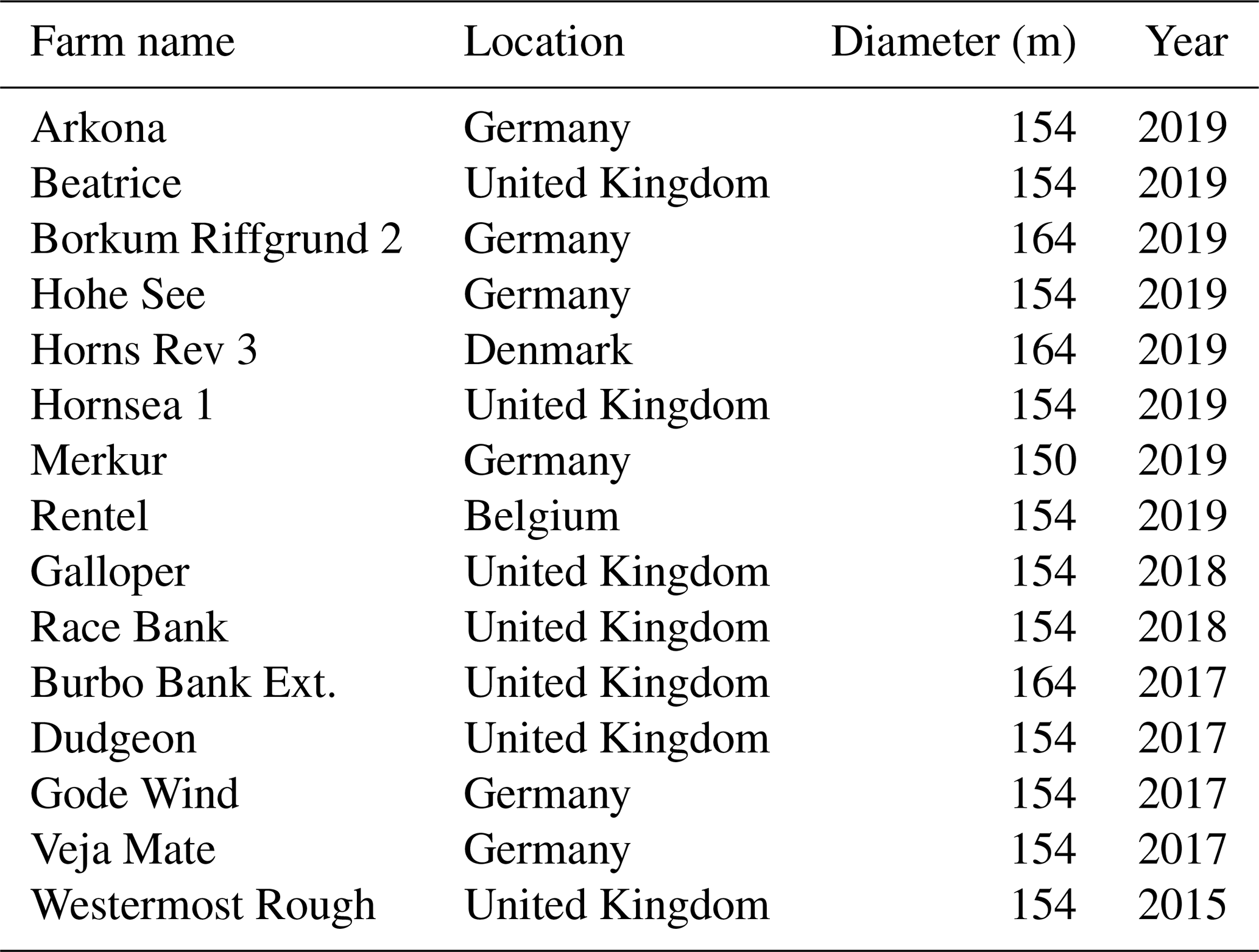
The coherence of turbulence is a measure for the spatial correlation of the velocity fluctuations in the incoming wind field (Panofsky and McCormick, 1954) and is one of the key parameters for the estimation of wind turbine loads. In wind engineering, the modelling of the coherence is required to design structures with dimensions much larger than the size of the eddies (Davenport, 1962), such as long-span bridges and high-rise buildings but also wind turbines. The continuously increasing rotor diameter of state-of-the-art wind turbines has motivated the growing interest toward an improved characterization of the coherence (e.g. Saranyasoontorn et al., 2004; Kelley et al., 2005; Bachynski and Eliassen, 2019; Doubrawa et al., 2019). Commissioned offshore wind turbines with a rotor diameter larger than 150 m have been deployed since 2015, and their number has been increasing (Table 1). Even larger diameters are currently developed, such as the GE's Haliade-X wind turbine, which has a diameter of 220 m. Such dimensions challenge the traditional modelling of the coherence, which relies often on onshore measurements from meteorological masts, typically not covering the full spatial extent of modern wind turbines. The poor data coverage at altitudes relevant to offshore wind turbines, i.e. from 50 to 200 m above sea level (a.s.l.), has been identified as one major challenge for wind energy research (Veers et al., 2019).

For wind turbine design, the spatial correlation of eddies needs to be assessed both in terms of vertical and lateral coherence. The lateral coherence refers herein to the coherence of any of the three wind velocity components, in the horizontal plane and in the crosswind direction. The vertical coherence refers to vertical separations.

Linear arrays of met masts have been used since the 1970s to study the lateral coherence above land (e.g. Pielke and Panofsky, 1970; Ropelewski et al., 1973; Perry et al., 1978; Peng et al., 2018). In the marine atmospheric boundary layer (MABL), much less information is available. In coastal sites, the lateral coherence has been studied using masts mounted on an islet (Mann, 1994) or an island (Andersen and Løvseth, 2006). However, many offshore sites are free of them, and the installation cost can become prohibitive if the mast structure must be anchored to the seabed.

Table 1 List of offshore wind farms with commissioned wind turbines having a rotor diameter larger than 150 m.

The rising popularity of affordable commercial Doppler wind lidars (DWLs) has opened up a new opportunity to study the lateral coherence of offshore wind. Although the possibility to use DWLs to study the coherence was already mentioned at the end of the 1980s by Kristensen et al. (1989), the first full-scale measurements were conducted onshore during the 2000s only (e.g. Lothon et al., 2006). For the past 10 years, multiple synchronized lidars have been deployed during pilot campaigns to study the lateral coherence (Cheynet et al., 2016a, 2017b; Letson et al., 2019), but none of them attempted to capture it in an offshore environment. During the OBLEX-F1 campaign, the lateral coherence was assessed above the sea using a single pulsed DWL and plan-position-indicator sector scans (Cheynet et al., 2016b). The use of a single scanning lidar means that a relatively low sampling frequency, around 0.20 Hz, was used and that the scanning beams were not truly parallel.

The present study introduces a multi-lidar setup to investigate the characteristics of offshore wind coherence from DWLs located onshore. The instruments were deployed between 2019 and 2020, as part of the COTUR campaign (COherence of TURbulence with lidars). COTUR was a joint research project developed and carried out by NORCE, the University of Bergen, the University of Stavanger and Equinor. The main objective of COTUR was to assess how multiple synchronized DWLs can be utilized to characterize the lateral coherence of turbulence above the sea, at altitudes close to the hub height of large offshore wind turbines. Therefore, the measurement campaign may improve the understanding of the second-order structure of turbulence above the ocean. In this regard, the project complements recent studies of offshore wind measurement from remote sensing instruments on land (e.g. Floors et al., 2016).

The project utilized three synchronized long-range Doppler scanning lidar systems deployed on the seaside to study the lateral coherence of the wind above the ocean, at a distance up to 2 km from the coast. The scanning beams of the lidars were aligned automatically every hour into the mean wind, using the wind direction measured by an additionally deployed Doppler lidar wind profiler. To supplement the lidar measurements, a passive microwave radiometer was deployed to record vertical temperature and humidity profiles through the boundary layer. During the last 2 weeks of the campaign, two masts equipped with one 3D ultrasonic anemometer each were deployed north to the measurement site to validate the ability of the lidar setup to capture the coherence of turbulence.

The paper is organized as follows: Sect. 2 outlines the COTUR campaign and the measurement strategy; Sect. 3 provides an overview of the data availability and describes how the lateral coherence is studied using parallel scanning beams. Finally, Sect. 4 illustrates the potential of the data set for future research.

2 The COTUR campaign

2.1 Site description

The COTUR campaign took place between February 2019 and April 2020 in a coastal area, at Obrestad Lighthouse, in southwestern Norway. Several sites on the Norwegian coast were considered for the measurement campaign. The most important criteria were (i) the local wind conditions, preferably westerly winds with large fetch over the ocean; (ii) the absence of mountains close to the coast, which may disturb the flow at a mesoscale level; (iii) ease of access to the measurement site; and (iv) availability of electricity and broadband internet.

Figure 1 Location of the Obrestad Lighthouse on the southwest coast of Norway with a sketch of the three Doppler wind lidars named LidarS, LidarN and LidarW pointing toward a direction of 300^∘.

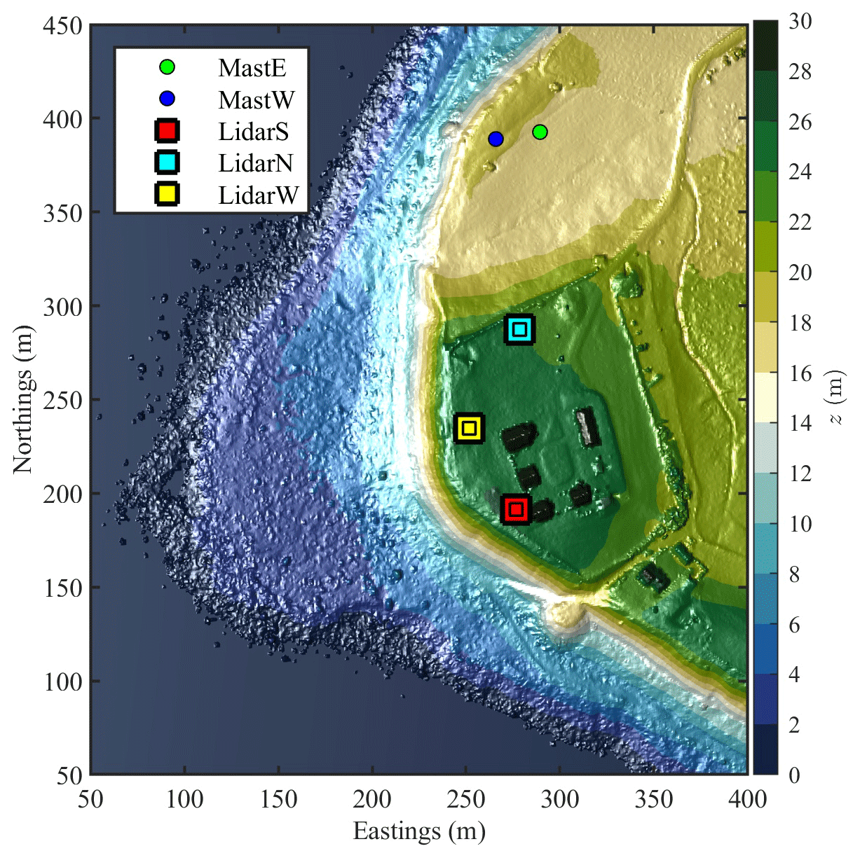
Figure 2 Local topography at the measurement site, obtained from a digital surface model generated using airborne laser instruments with a horizontal resolution of 1 m.

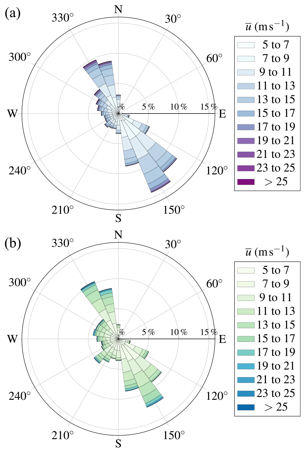
Figure 3 Wind roses computed using 10 min mean wind records from 1990 to 2020 (a) and from March 2019 to March 2020 (b), 10 m above the ground by the Obrestad Lighthouse weather station. Only samples associated with $\stackrel{\mathrm{‾}}{u}\ge \mathrm{5}$ m s⁻¹ are considered for the sake of clarity.

Obrestad Lighthouse, located 50 km south of the city of Stavanger (Fig. 1), was found to be the most suitable site for this campaign. The topography behind the lighthouse is relatively flat up to 10 km inland. The site was chosen for its good exposure to strong seaward winds combined with easy access from the road. This ensured that the installed DWLs and the radiometer could be continuously operated, remotely monitored and physically accessed for maintenance during the campaign.

The lighthouse is situated on a small plateau 25 m a.s.l., to the east of an escarpment with steep slopes between 25^∘ and 35^∘ (Fig. 2), which can modify the static and dynamic flow characteristics at a microscale level. This escarpment is twice as high as the Bolund hill, which was extensively studied to improve the modelling of atmospheric flow in complex terrains (e.g. Berg et al., 2011; Bechmann et al., 2011; Lange et al., 2016; Ma and Liu, 2017). Results from the Bolund hill experiments suggest that the escarpment at Obrestad Lighthouse might affect the local flow characteristics up to 50 m above the instruments. The influence of the coastline on low-frequency velocity fluctuations, i.e. a timescale from 1 to 10 min, may be noticeable up to several hundred metres away from the shore (Emeis et al., 1995). Therefore, the use of long-range scanning Doppler wind lidar instruments is justified to study the flow conditions up to 2 km from the seaside.

Long-term records from a weather station located at Obrestad Lighthouse and operated by the Norwegian Meteorological Institute indicate that the wind blows generally either from the northwest or southeast, i.e. parallel to the coast (Fig. 3). The wind direction distribution during the experimental campaign (March 2019–March 2020) is consistent with the climatological records (1990–2020). This includes winds in the 180–270^∘ sector, which are favourable for the COTUR experiment. These flow conditions happened 20 % of the time between March 2019 and March 2020 against 15 % for the 30-year reference median value. Such directions were desirable to remotely study offshore wind conditions from the instruments located onshore.

2.2 Instrumentation

2.2.1 Doppler wind profiler Leosphere WindCube V1

The vertical profiles of the mean wind speed and mean wind direction at the Obrestad Lighthouse were recorded by a Leosphere WindCube V1 profiling lidar (Fig. 4). The WindCube V1 measurement principle is based on a Doppler beam swinging (DBS) scanning pattern: the lidar emits a series of near-infrared light pulses (λ≈1.54 µm) along four directions, where the azimuth of each beam is shifted by 90^∘. All four beams have a fixed elevation angle of 62^∘. The term “elevation angle” refers herein to the angle located in the vertical plane, between the line of sight and the horizontal plane. The “azimuth” refers to the angle located in the horizontal plane, measured from north in a clockwise direction. Along the line of sight (LOS) of the individual beams, the lidar obtains the radial velocity component from a Doppler shift of the beam, triggered by the interactions of the beam with aerosol particles that are moving with the wind. One DBS scan provides four radial wind speed values at each measurement height, which is solvable in terms of the three-dimensional wind vector (Werner, 2005).

2.2.2 Scanning Doppler wind lidar Leosphere WindCube 100S

The three scanning lidar instruments are of the type WindCube 100S from Leosphere (https://www.leosphere.com, last access: 20 December 2020). They were deployed in a triangular setup where the northern instrument is named LidarN, the southern one is LidarS and the western one is LidarW (Figs. 2 and 4). These instruments are pulsed Doppler wind lidars equipped with a scanner head that can orient the laser beam with an azimuth from 0 to 360^∘ and an elevation angle from −10 to 190^∘. The scanning instruments were installed on top of measurement platforms constructed of Bosch Rexroth aluminium strut profiles (Fig. 4). Both LidarW and LidarS were installed 2 m above ground, whereas the LidarN was installed 3 m above ground to account for the slightly lower terrain at this instrument position (Fig. 2). Therefore, the scanner heads of all three instruments were located approximately 28 m a.s.l. Finally, the location of the lidar instruments was measured by Global Navigation Satellite System (GNSS) and theodolite sightings.

Figure 4 The main instrumental site of the COTUR campaign with one of the scanning lidars, Leosphere WindCube 100S (LidarN) in the centre, the Leosphere WindCube V1 wind profiler to the right, and the Radiometer Physics HATPRO RG4 passive microwave temperature and humidity profiler to the left. The picture was taken towards north-northwest.

The study of two-point turbulence characteristics from three individual scanning lidar measurements requires the instruments to be synchronized in time. Synchronized DWLs were developed within the WindScanner.dk research infrastructure (Mikkelsen et al., 2008), which was later ramified into the long-range and the short-range WindScanner systems (Mikkelsen, 2014; Vasiljevic, 2014). For the COTUR project, the long-range WindScanner system was utilized.

The long-range WindScanner client software developed by the Technical University of Denmark (DTU; Vasiljević et al., 2016) runs on the individual lidar computers and controls the scanner motion and the laser shots according to scenarios that are received from a master control software that can run on a remote PC. The master control software can send synchronized scenarios to multiple systems and monitors the synchronicity of all systems connected. The collected data are stored on both the client and the master PC. The master and client software communicate through the RSComPro protocol (Vasiljevic and Trujillo, 2014).

For advanced programming of scanning scenarios and monitoring of the measurements on a virtual globe, especially for multi-Doppler measurements, the Institute of Atmospheric Physics of the German Aerospace Center (DLR) developed an alternative master control software (LidarPlanner) featuring the RSComPro protocol. An important feature of the LidarPlanner is that it allows reading a wind direction from an external file and, upon retrieval of a new value, automatically generates modified scanning scenarios based on this information. The modified scenarios are then uploaded to the lidars and measurements are restarted. Wildmann et al. (2018) used this feature to calculate the lidar parameters for intersecting beams and triple-Doppler measurements in the wake of a wind turbine depending on the wind direction. In COTUR, the azimuth of the lidar scenarios was simply adjusted to point all three systems into the mean wind direction, obtained from 10 min records by the WindCube V1.

2.2.3 Passive microwave temperature and humidity profiler Radiometer Physics HATPRO RG4

To investigate the structure of the atmospheric boundary layer at the measurement site, an RPG Radiometer Physics GmbH (RPG) humidity and temperature profiler generation 4 (HATPRO-G4) passive microwave radiometer (Rose and Czekala, 2014) was installed next to LidarN. The HATPRO-G4 measurements rely on detecting the radiation emitted by the atmosphere at selected frequencies of the microwave spectrum.

The HATPRO-G4 measures simultaneously brightness temperatures at 14 frequencies divided into two bands ranging from 22.24 to 31.40 GHz (K-band) and 51.26 to 58.00 GHz (V-band) for sensing humidity and temperature profiles, respectively (Rose et al., 2005; Rose and Czekala, 2014).

The atmosphere microwave (MW) emission is received at the radiometer's antenna along the instrument field of view. As the radiometer senses MW radiations that contain indirect information about the columnar distribution of temperature and humidity, profiles are retrieved based on the spectral information and observed elevation angles. The profiles of the atmospheric temperature and humidity were retrieved up to 10 km with non-uniform vertical spacing. In the first 1200 m above the surface, the vertical measurement resolution ranged from 25 to 40 m, whereas above 1200 m, it ranged from 50 to 300 m.

The HATPRO-G4 proprietary software provides three retrieval methods, i.e. linear regression, quadratic regression and neural networks. For COTUR, retrievals were based on neural networks by RPG's firmware training data of temperature, humidity and pressure recorded from radiosondes launched at Værnes, Sola and Ekofisk stations. An in-house retrieval algorithm was utilized for cases where the RPG firmware retrieval database did not represent properly the atmospheric conditions (Saavedra and Reuder, 2019). During the COTUR campaign, the HATPRO-G4 was installed with its field of view bearing westerly towards the open sea (Fig. 4 left) and was operated in boundary layer sensing mode with 10 elevation angles from 4.2 to 90^∘ every 5 min.

2.2.4 Sonic anemometers on hydraulic masts

From the 16 to 29 March 2020, two telescopic meteorological masts PT180-6-NC from Clark Masts were deployed in an open area, 20 m from each other, ca. 100 m north to LidarN (Fig. 5). The masts were equipped with spirit levels to ensure that the anemometers were mounted horizontally. Each mast was instrumented with one sonic anemometer on its top (Fig. 5), approximatively 11 m above ground. The measurement volumes of these anemometers were, therefore, located ca. 28 m a.s.l. These additional measurements aimed to compare turbulence characteristics estimated by the scanning lidars with those estimated from the sonic anemometers. The anemometers are Gill WindMaster sonic anemometers operating at a sampling frequency of 20 Hz. The scanning beams of LidarN and LidarW were orientated towards each mast at a fixed azimuth of 5.3^∘ and a zero elevation angle, such that their beams were parallel and horizontal. The choice of azimuth resulted in beams almost intersecting with the anemometer location on each mast.

A northerly or southerly wind direction offered suitable conditions for comparison between the sonic anemometers and the lidars data as the flow was approximately parallel to the lidar beams. The potential effect of the terrain on the local flow conditions was more limited for northerly winds, which were found to be best suited to validate the ability of the lidars to capture the lateral coherence of turbulence.

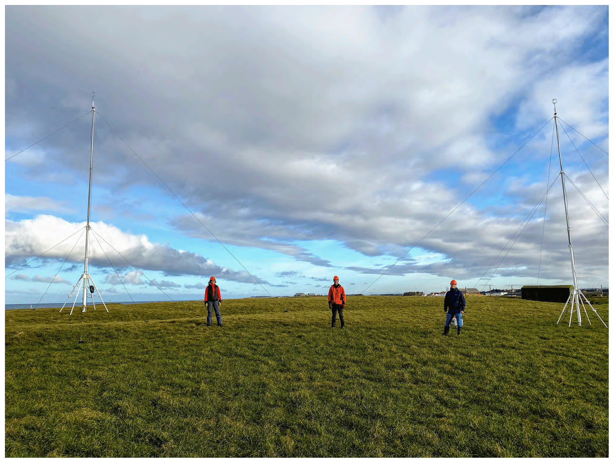
Figure 5 Telescopic masts mounted in a field, approximately 100 m north to LidarN, separated by 20 m from each other and equipped with one 3D sonic anemometer on their top at a height of 11 m above ground level.

3 Method

3.1 Measurement and scanning strategy

To study the horizontal coherence, the scanning lidars operated in a fixed line-of-sight (LOS) scanning mode, i.e. with a fixed azimuth and elevation angle. To include as many turbulence scales as possible and to reduce the statistical uncertainties associated with the coherence estimates, the scan duration was set to 50 min.

The LOS scans were performed with a pulse length of 100 ns, a window size of 64 points for the fast-Fourier transform, a pulse repetition rate of 40 kHz and an accumulation time of 1 s. This corresponds to a sampling frequency of 1Hz and a probe volume of approximately 25 m length. The range gates were set to 25 m with a maximal scanning distance of 1975 m, resulting in 78 range gates. The azimuth, which corresponded to the last reported 10 min averaged wind direction at 75 m above the ground, i.e. approximatively 100 m a.s.l., was provided by the WindCube V1 and updated before the start of each new LOS scan.

As the campaign aimed to study atmospheric turbulence for wind energy applications, the LOS scans were performed with three predefined elevation angles of 2.0, 3.4 and 4.9^∘. At a distance of 1200 m from the lidar locations, these angles correspond to altitudes of 70, 100 and 130 m, respectively. Considering the case of a large offshore wind turbine positioned at a distance larger than 1 km from the shore, the choice of these elevation angles permits the study of the flow over the typical extension of the rotor disc. With the chosen low elevation angles, potential contamination of the along-beam velocity component by the vertical wind component can be neglected.

Initially, the lidars were programmed to perform a repeating series of three consecutive LOS scans, where each scan used one of the three predefined elevation angles. Utilizing the WindScanner software, all three scanning lidars performed time-synchronized measurements with identical azimuth and elevation angles during each scan. For LOS scenarios, the three beams of the different scanning lidars were thus orientated parallel to each other.

Within the first month of the measurement campaign, it was discovered that the scanning lidars had a “homing” issue; i.e. the lidar's scanner head azimuth reference system was no longer calibrated with respect to true north. As a result of the lost homing, the laser beam of the scanning lidars was no longer pointing into the geographic azimuth direction (i.e. relative to true north) provided by the WindCube V1. Therefore, a series of short plan-position-indicator (PPI) scans were additionally programmed in which the lidar's respective laser beams were directed towards the top of the lighthouse. Since the geographic azimuth direction of the lighthouse's upper part was known for each of the respective scanning lidars, the PPI scans were used in the post-processing of the data to identify any period where one lidar had lost its homing. Whenever the lidars were operating with correct azimuths, the lighthouse was visible in the respective PPI scans due to range gate blending. To minimize the potential occurrence of the homing issue, the orientation of the lidar scanner heads was visually checked during the regular maintenance intervals. Furthermore, the Delta Tau Turbo PMAC motion controller (Hutson, 2018), which governs the motion of the scanner head, was reset whenever one of the lidars reported radial wind speeds and carrier-to-noise (CNR) values thoroughly different compared the other two scanning lidars. In November 2019, the WindCube V1 stopped operating due to water ingression into the instrument. To orientate the laser beams of the scanning lidars into the prevailing wind direction at 100 m a.s.l., the wind direction was derived from DBS scans performed with the scanning lidars themselves.

The WindCube V1 was programmed to simultaneously measure the mean wind speed at 10 vertical levels between 40 and 250 m above the instrument. The range gates were linearly spaced every 25 m, except at the lowest two measurement levels, where the range gates were 40 and 50 m above the instrument. One complete DBS scan takes approximately 4.6 s. The 10 min mean wind direction estimated 75 m above the WindCube V1, i.e. approximatively 100 m a.s.l., was used to align the laser beams of the three scanning Doppler wind lidar systems (Sect. 2.2.2) into the mean wind direction. This height was chosen to limit the influence of the escarpment on the local flow conditions and to consider velocity records as close as possible to the hub height of a multi-megawatt offshore wind turbine.

Therefore, the sequence of scan scenarios performed during the measurement campaign was (i) 50 min LOS scan at one of the predefined elevation angles followed by (ii) a series of short PPI scans, totally lasting 15 min, before advancing to a new LOS scan with a different azimuth and elevation angle. From November 2019, a 10 min DBS scan scenario was run after the PPI scan scenario to determine the 10 min mean wind direction at 100 m a.s.l., which served as updated azimuth input for the following LOS scan.

Due to the location of the lighthouse and the adjacent buildings, the scanning lidars were installed in a triangular setup, with unequal longitudinal and lateral distances between the instruments (Fig. 2). Consequently, for LOS scan scenarios, the lateral separation between the lidar's laser beams was a function of the geographic azimuth and thus depended on the wind directions. As the buildings partially limited the lidar's LOS scan view towards easterly to southerly directions, the lidar laser beams were orientated into the mean wind direction for winds blowing within the free view sector 190 to 350^∘, and they were orientated into the opposite mean wind direction for winds coming from all other directions when performing LOS scans. Note that buildings prevented LidarN from performing LOS scans towards south.

3.2 Lidar data processing for coherence analysis

Although the majority of the performed LOS scan scenarios have a duration of 50 min, instrument acquisition errors led occasionally to loss of data and resulted in time series that were shortened. In the MABL, turbulence characteristics are typically studied using records equal to or longer than 30 min (Smith, 1980; Andersen and Løvseth, 2006; Cheynet et al., 2018). This aims to ensure that a sufficiently large number of eddies pass through the instrument measurement volume for precise estimation of the flow characteristics (Lumley and Panofsky, 1964; Kaimal and Finnigan, 1994). Therefore, collocated LOS scan scenario time series with a duration shorter than 30 min were dismissed.

Each instantaneous LOS velocity record is associated with a CNR value, which can be used to eliminate outliers. One straightforward approach relies on a fixed value of the CNR, generally between −24 and −28 dB, below which data are discarded. Some recent studies (Beck and Kühn, 2017; Valldecabres et al., 2018; Alcayaga, 2020) argue that setting a fixed threshold value for the CNR can cause exaggerated data removal, which can be a critical issue when the overall data availability is low. While Beck and Kühn (2017) and Valldecabres et al. (2018) used an iterative method based on a moving standard deviation window to increase the data availability, we used herein a two-stage method without iteration. The first stage aimed to “rescue” realistic velocity data with a CNR below −27.5 dB. This was achieved using the Mahalanobis distance (Mahalanobis, 1936), which describes how many standard deviations away a point is from the mean value of a distribution. In the present study, any point located at a Mahalanobis distance beyond 20 was considered as an outlier and dismissed. In addition, any measurements with a CNR below −35 dB was automatically removed (Fig. 6).

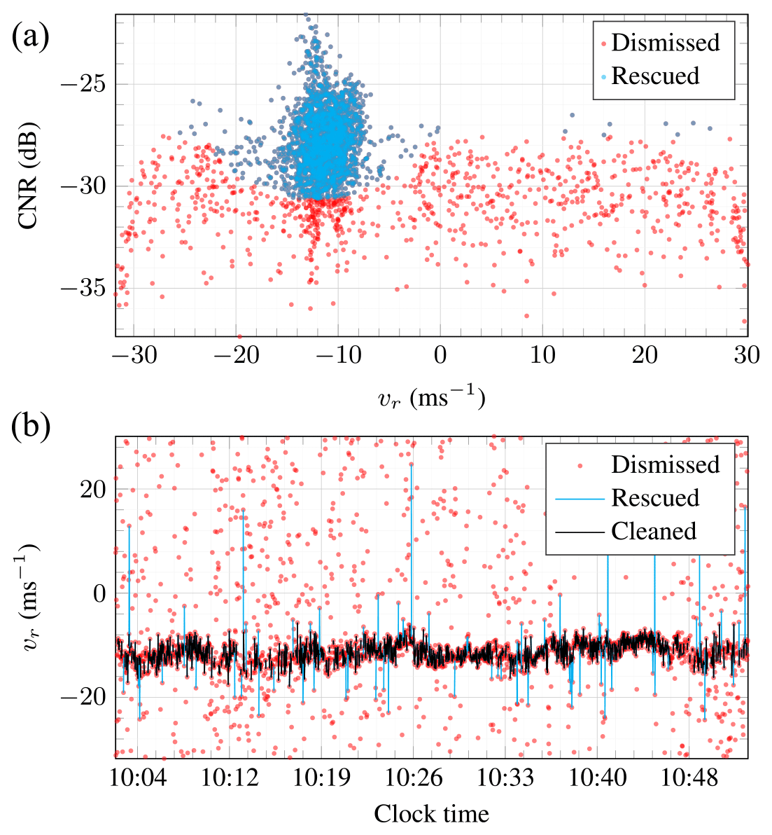
Figure 6 (a) Scatter plot of the CNR versus the along-beam velocity on 25 October 2019 from 10:03 to 10:52 for the range gate located 275 m away from the lidars. (b) Corresponding time series showing the dismissed and rescued samples using the Mahalanobis distance and the cleaned data after application of outlier analysis based on the median absolute deviation.

As shown in Fig. 6, not all the outliers are eliminated after the first stage. The second stage relies on an outlier detection algorithm relying on the absolute deviation around the median (Leys et al., 2013). A moving median filter with a window length of 200 s was applied to the time series. The resulting local median values were then used to compute the median absolute deviation (MAD) (Hampel, 1974; Leys et al., 2013). Any point that was more than three MAD away from the median was classified as an outlier.

The analysis of second-order turbulence characteristics requires stationary records. The first and second-order stationary assumptions were, therefore, assessed using the moving mean and moving standard deviation with a window length of 10 min. Samples with a maximal relative difference below 20 % between the static mean and moving mean and below 50 % between the static standard deviation and moving standard deviation were assumed to be stationary. The threshold value is larger for the second-order stationarity test, because second-order statistics have larger statistical uncertainties than first-order statistics for the same averaging time. The relatively large threshold value of 50 % is chosen as the coherence is less sensitive to non-stationary fluctuations than one-point turbulence characteristics (Chen et al., 2007). Using this approach, approximately 35 % of the time series available for analysis were detected as non-stationary.

3.3 Coherence modelling

The spatial correlation of the velocity records is assessed at different wavenumbers (or frequencies) using the lateral and longitudinal coherence, i.e. the coherence in the crosswind (y axis) and along-wind direction (x axis), respectively.

The root coherence of the along-wind component u between two points located in a horizontal plane, at coordinates (x₁,y₁) and (x₂,y₂), is defined as

$$\begin{array}{}\text{(1)}& {\displaystyle }{\mathrm{coh}}_u(x_{\mathrm{1}},y_{\mathrm{1}},x_{\mathrm{2}},y_{\mathrm{2}},f){\displaystyle }={\displaystyle \frac{S_u(x_{\mathrm{1}},y_{\mathrm{1}},x_{\mathrm{2}},y_{\mathrm{2}},f)}{\sqrt{S_u(x_{\mathrm{1}},y_{\mathrm{1}},f)S_u(x_{\mathrm{2}},y_{\mathrm{2}},f)}}},\end{array}$$

where $S_u(x_{\mathrm{1}},y_{\mathrm{1}},x_{\mathrm{2}},y_{\mathrm{2}},f)$ is the two-point cross-spectral density of the u component, and $S_u(x_{\mathrm{1}},y_{\mathrm{1}},f)$ and $S_u(x_{\mathrm{2}},y_{\mathrm{2}},f)$ are the one-point spectra of the u component measured at the locations (x₁,y₁) and (x₂,y₂), respectively.

In the following, the assumption of homogeneous turbulence implies that the root coherence is expressed as a function of the spatial separations d_x and d_y instead of the spatial coordinates, i.e.

$$\begin{array}{}\text{(2)}& {\displaystyle }{\mathrm{coh}}_u(x_{\mathrm{1}},y_{\mathrm{1}},x_{\mathrm{2}},y_{\mathrm{2}},f)\approx {\mathrm{coh}}_u(d_x,d_y,f),\end{array}$$

where $d_x=\left|x_{\mathrm{1}}-x_{\mathrm{2}}\right|$ and $d_y=\left|y_{\mathrm{1}}-y_{\mathrm{2}}\right|$ are the longitudinal and lateral separations, respectively.

The root coherence is a complex-valued function, the real part of which is the co-coherence and denoted γ_u, whereas its imaginary part, called quad-coherence, is denoted ρ_u. As highlighted by ESDU 86010 (2002), the co-coherence and quad-coherence can be written as

$$\begin{array}{}\text{(3)}& {\displaystyle }{\mathit{\gamma }}_u(d_x,d_y,f)& {\displaystyle }=\left|{\mathrm{coh}}_u\right(d_x,d_y,f\left)\right|\cos \left({\mathit{\varphi }}_x+{\mathit{\varphi }}_z\right),\text{(4)}& {\displaystyle }{\mathit{\rho }}_u(d_x,d_y,f)& {\displaystyle }=\left|{\mathrm{coh}}_u\right(d_x,d_y,f\left)\right|\sin \left({\mathit{\varphi }}_x+{\mathit{\varphi }}_z\right),\end{array}$$

where ${\mathit{\varphi }}_x\approx \frac{\mathrm{2}\mathit{\pi }f{d}_x}{\stackrel{\mathrm{‾}}{u}}$ is a phase angle associated with a time lag $d_t=\stackrel{\mathrm{‾}}{u}/d_x$ between two measurement locations. The phase angle ϕ_z reflects the presence of wind shear due to the blocking by the ground. It is generally negligible, except for the lateral velocity component at vertical separations (Bowen et al., 1983; ESDU 86010, 2002). The term ϕ_z is, therefore, disregarded in the present study as only horizontal separations are studied.

The most straightforward approach to study the horizontal root coherence of natural wind is to use at least two anemometers, at the same measurement height, located along a line perpendicular to the wind direction (Shiotani, 1969; Pielke and Panofsky, 1970; Ropelewski et al., 1973). In the case of anemometers mounted on masts, the wind direction is not always normal to the linear sensor array. In this situation, the yaw angle, defined as the angle between the wind direction and the normal to the sensor array, is different from zero. As the distance d between two anemometers becomes larger than the corresponding crosswind distance d_y (Fig. 7), the longitudinal distance d_x becomes non-zero, which leads to ϕ_x≠0 and a non-zero quad-coherence. Although the quad-coherence does not participate directly in the linearized dynamic load on slender structures in frequency-domain approaches, it should be accounted for in time-domain approaches for strongly skewed wind field simulations. As the present study does not focus on skewed flow conditions, only the co-coherence is discussed herein.

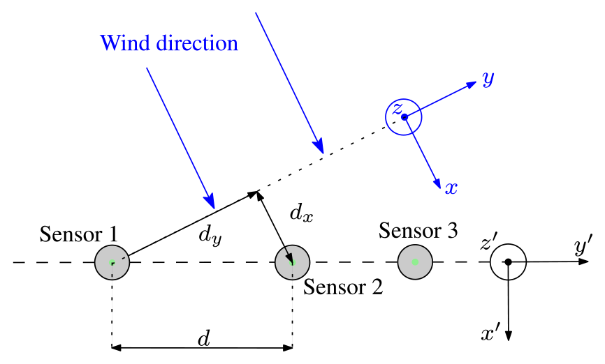
Figure 7 Sketch of a typical configuration of three anemometers (sensors 1, 2 and 3) mounted at the same height along a linear array of masts to study the lateral co-coherence of wind. This sketch is used for illustrative purpose only and does not reflect the instrumentation of the COTUR campaign.

For a flow direction normal to a linear array of sonic anemometers (ϕ_x≈0), the root coherence of natural wind can be empirically described using an exponential decay (Davenport, 1961; Pielke and Panofsky, 1970)

$$\begin{array}{}\text{(5)}& {\displaystyle }{\mathit{\gamma }}_u(d_y,f){\displaystyle }\approx \exp \left({\displaystyle \frac{-C_y{d}_{y}f}{\stackrel{\mathrm{‾}}{u}}}\right),\end{array}$$

where C_y is an empirically determined decay coefficient, f is the frequency in Hz and $\stackrel{\mathrm{‾}}{u}$ is the mean wind speed averaged between each pair of sensors.

Although the Davenport model has no theoretical foundation, it is widely used for its simplicity, especially for engineering applications. For wind turbine design, it is the fundamental model upon which more advanced models are built and applied to e.g. synthetic turbulence generation (Jonkman, 2009). In wind engineering, the study of the coherence is motivated by the need to assess the Davenport decay coefficients C_y and C_z for lateral and vertical separations, respectively. When measured on-site, these coefficients may substantially differ from the values provided in standards and codes. Lower decay coefficients imply a larger co-coherence, i.e. larger eddies and an increased turbulent wind load on structures. Therefore, improved decay coefficient estimates could lead either to substantially reduced construction costs or more robust designs.

Using Taylor's hypothesis of frozen turbulence (Taylor, 1938), one can assume that the root coherence is equal to unity in the along-wind direction. Therefore, combining Eqs. (5 and (3) leads to

$$\begin{array}{}\text{(6)}& {\displaystyle }{\mathit{\gamma }}_u(d_x,d_y,f){\displaystyle }\approx \exp \left({\displaystyle \frac{-C_y{d}_{y}f}{\stackrel{\mathrm{‾}}{u}}}\right)\cos \left[{\displaystyle \frac{\mathrm{2}\mathit{\pi }{d}_{x}f}{\stackrel{\mathrm{‾}}{u}}}\right].\end{array}$$

Note that there exist alternative coherence models based on the spectral tensor of homogeneous turbulence (e.g. Kristensen et al., 1989; Mann, 1994), but these cannot easily be assessed using long-range scanning lidar instruments measuring the along-wind component only. Therefore, these models are not discussed herein.

Taylor's hypothesis can be relaxed using an additional decay coefficient C_x≠0, reflecting the time-varying characteristics of eddies as they are advected in the along-wind direction. Studying the value of C_x provides additional information on the structure of turbulence. A refined model to study the co-coherence in the horizontal plane is, therefore,

$$\begin{array}{}\text{(7)}& {\displaystyle }{\mathit{\gamma }}_u(d_x,d_y,f)& {\displaystyle }\approx \exp \left(-{\displaystyle \frac{f}{\stackrel{\mathrm{‾}}{u}}}D\right)\cos \left[{\displaystyle \frac{\mathrm{2}\mathit{\pi }{d}_{x}f}{\stackrel{\mathrm{‾}}{u}}}\right]\text{(8)}& {\displaystyle }D& {\displaystyle }=\sqrt{(C_x{d}_x{)}^{\mathrm{2}}+(C_y{d}_y{)}^{\mathrm{2}}}.\end{array}$$

For a given turbulence length scale in the lateral direction L_y, the Davenport model is usually valid if $d_y/L_y\ll \mathrm{1}$, which is no longer the case at large crosswind separations (Irwin, 1979; Kristensen and Jensen, 1979). To account for the limited size of the eddies in the lateral direction, additional decay coefficients could be introduced, but these were found small enough to be neglected in the present study.

It is unclear whether C_y can be derived from the knowledge of C_z. Both decay coefficients depend likely on the atmospheric stability and the terrain roughness (Ropelewski et al., 1973; Soucy et al., 1982; Cheynet et al., 2018). Schlez and Infield (1998) suggested that for a given turbulence intensity, the decay coefficient of the lateral co-coherence is independent of the mean wind speed. In the surface layer, the dependence of the decay coefficients on the spatial separation and measurement height has been highlighted for both lateral and vertical separations (Kanda and Royles, 1978; Perry et al., 1978; Shiotani et al., 1978; Kristensen et al., 1981; Cheynet et al., 2017b; Bowen et al., 1983; Cheynet, 2018), reflecting the increase in the size of the eddies further away from the ground.

Equation (7) is a two-parameter function where C_x and C_y need both to be determined from measurements. Using synchronized pulsed DWL instruments, the coefficients C_x and C_y can be either simultaneously or independently estimated using a least-squares fit of Eq. (7) to the co-coherence estimate.

The simultaneous identification of C_x and C_y is attractive if the elevation angles are different from zero. To minimize the influence of the vertical separation on the estimated decay coefficients, the range gates associated with the lowest vertical separations need to be selected. However, the final value of C_x can be sensitive to the initial guess. The separate estimation of C_x and C_y is more cumbersome but also more robust if $d_z/d_x\ll \mathrm{1}$. This second approach is possible using pulsed DWLs which provide simultaneous measurements along the scanning beams. In particular, the coefficient C_x can be estimated using a single lidar instrument. Once C_x is identified, the second coefficient C_y can be obtained by least-squares fitting Eq. (7) to the horizontal co-coherence. However, if the elevation angle is substantially different from zero, the coefficient C_x can be estimated with a large bias. Therefore, for the preliminary data analysis shown in this article (Sect. 4), the simultaneous fitting of the decay coefficients is adopted.

Due to the triangular setup of the scanning lidars in COTUR, the measurement volumes were not co-located in the crosswind direction even though the laser beams were directed into the mean wind direction. Denoting the centre of two volumes in a horizontal plane as A₁ and A₂ (Fig. 8), their along-wind and crosswind separations are d_x and d_y. This situation can be related to the case of an array of sonic anemometers recording a flow with a yawed wind direction (Fig. 7). Using the aforementioned lidar setup (Sect. 2.2), the co-coherence can be studied using Eq. (7) and the GPS position of the scanning instruments to estimate the distances d_x and d_y between each range gate. Finally, the requirement of stationary fluctuations was fundamental to ensure that the scanning beams were parallel to the mean wind direction as the azimuth was updated once every hour only.

Figure 8 Schematic of the distances d_x and d_y defined by the two closest range gates for a given scanning distance.

The co-coherence is generally estimated with large uncertainties if a single time series is used. These uncertainties can be reduced if low spatial separations are considered, i.e. crosswind distances typically below 25 m or by increasing the averaging time. Another alternative is to increase the spatial resolution by simultaneously measuring the flow in a large number of locations, as in Cheynet et al. (2016a), where the lateral co-coherence was estimated using 26 measurement volumes. The statistical uncertainties can also be reduced using an appropriate power spectral density (PSD) estimate. In the present study, the co-coherence was computed using Welch's algorithm (Welch, 1967) with multiple segments and 50 % overlapping. To assess the sensitivity of the co-coherence estimates on the number of segments and, therefore, on their duration, the co-coherence was computed with segments of 90 to 600 s. Negligible differences were found between the different segment lengths, and a value of 300 s was finally chosen as a compromise between frequency resolution and smoothness of the co-coherence estimates.

The probe volume averaging modifies the estimation of the co-coherence since the scanning beams cannot be perfectly aligned with the instantaneous wind direction. Nevertheless, the resulting spatial averaging effect may have a limited influence on the co-coherence estimation, since the latter relies on a normalization of the two-point cross PSD by the one-point PSD densities (Cheynet et al., 2016a). On the other hand, Debnath et al. (2020) suggested that the spatial averaging may lead to an over-prediction of the magnitude coherence in the low-frequency range if the probe volume is substantially larger than a typical length scale of turbulence. Further studies are, therefore, required to clarify the influence of the probe volume averaging on the estimation of the coherence.

3.4 Pointing accuracy

For the present instrumental setup and the study of the co-coherence, the pointing error for the azimuth and elevation angles should be below 0.1^∘, which is achievable with the WindCube 100S and the WindScanner system (Vasiljević et al., 2016). However, because the azimuth changes every 50 min, the lateral distance between the scanning beams changes also with the wind direction. Therefore, the pointing error influences directly the relative error on d_x and d_y as well as the Davenport decay coefficients.

The terms “azimuth offset” and “elevation offset” refer herein to an angular deviation from a reference azimuth and elevation angle, respectively. For a negligible elevation offset, the error ${\mathit{ϵ}}_{d_y}$ on the crosswind distance due to an azimuth offset ϵ_az increases with the scanning distance as

$$\begin{array}{}\text{(9)}& {\displaystyle }{\mathit{ϵ}}_{d_y}{\displaystyle }=r\sin \left({\mathit{ϵ}}_{az}\right).\end{array}$$

Denoting $\stackrel{\mathrm{̃}}{d_y}$ the crosswind distance affected by an azimuth offset, the biased decay coefficient $\stackrel{\mathrm{̃}}{C_y}$ is

$$\begin{array}{}\text{(10)}& {\displaystyle }\stackrel{\mathrm{̃}}{C_y}{\displaystyle }=C_y{\displaystyle \frac{d_y}{\stackrel{\mathrm{̃}}{d_y}}},\end{array}$$

and the relative error on the decay coefficient is

$$\begin{array}{}\text{(11)}& {\displaystyle }{\mathit{ϵ}}_{C_y}{\displaystyle }={\displaystyle \frac{\stackrel{\mathrm{̃}}{C_y}}{C_y}}-\mathrm{1}.\end{array}$$

Therefore, converging beams ($\stackrel{\mathrm{̃}}{d_y}<d_y$) will be associated with an overestimated decay coefficient, and diverging beams ($\stackrel{\mathrm{̃}}{d_y}>d_y$) will be associated with an underestimated decay coefficient. Assuming an azimuth offset of $\pm \mathrm{0.1}{}^{\circ }$ for LidarN and considering only LidarN and LidarW with a scanning distance of 1975 m, the lateral separation d_y=20 m is estimated with an accuracy of ±3 m (Eq. 9). The relative error ${\mathit{ϵ}}_{C_y}$ on the Davenport decay coefficient is up to 17 %. This error is acceptable when studying the co-coherence as the other sources of uncertainties can lead to relative errors ${\mathit{ϵ}}_{C_y}$ larger than 20 %. The various sources of uncertainties partly explain the large range of decay coefficients values reported by Solari and Piccardo (2001) for flat and homogeneous terrain.

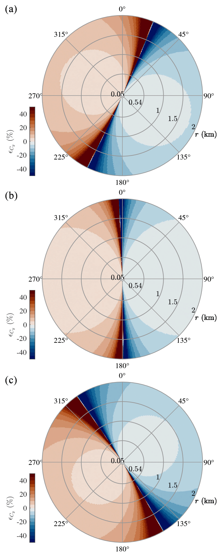
Figure 9 Relative error ${\mathit{ϵ}}_{C_y}$ on the Davenport decay coefficient C_y between LidarN and LidarW (a), LidarN and LidarS (b), and LidarW and LidarS (c), assuming an azimuth offset of $-\mathrm{0.1}{}^{\circ }$ for one of the two lidars selected. This relative error is independent on the value of C_y. The colour map was taken from Crameri (2018).

For an azimuth offset of $-\mathrm{0.1}{}^{\circ }$ for LidarN (or LidarS) due to a limited pointing accuracy, there exist some sectors where the co-coherence is associated with large uncertainties. For the pair LidarN–LidarW, Fig. 9 shows that ${\mathit{ϵ}}_{C_y}$ can be large when the wind direction is between 200 and 215^∘ and between 15 and 30^∘ because the distance between the scanning beams is similar to or smaller than the measurement uncertainty. Therefore, wind blowing with these directions cannot be used to study the lateral co-coherence of turbulence between LidarN and LidarW. For the same azimuth offset, the wind direction preventing the study of the coherence between LidarN and LidarS is either between 350 and 360^∘ or between 175 and 185^∘. The sectors that lead to unreliable co-coherence estimates between LidarW and LidarS are from 141 to 161^∘ and from 313 to 333^∘. In Fig. 9, the positive relative error implies that the scanning beams are converging, whereas negative errors reflect diverging beams.

In summary, the estimation of the Davenport decay coefficient is sensitive to several parameters: (1) the accuracy of the alignment between the lidar beams, (2) the consistency between the measured mean wind direction onshore and offshore, (3) the spatial averaging effect introduced by the probe volume, (4) the sampling frequency, (5) the spatial separation, (6) the range of frequencies considered for fitting, (7) the noise-to-signal ratio of the velocity data, which increases with the scanning distances, (8) the synchronization of the time series by a common clock time, (9) the number of sensors simultaneously considered (two or three lidars), (10) the local atmospheric stability, and (11) the measurement height. However, a detailed analysis of the sources of errors and their implication on the decay coefficients is out of the scope of the study.

3.5 Assessment of the atmospheric stability

Turbulence characteristics in the MABL are also sensitive to the thermal stratification of the atmosphere (e.g. Cheynet et al., 2018). However, assessing the atmospheric stability above the sea from sensors located onshore is challenging. In the present study, the bulk Richardson number Ri_b was used to calculate the dimensionless stability parameter $\mathit{\zeta }=z{L}^{-\mathrm{1}}$, where L is the Obukhov length. The sea-surface temperature, mean wind speed measurements from the scanning wind lidars and temperature profile data collected by the HATPRO radiometer were used to estimate Ri_b. The sea-surface temperature was obtained a couple of kilometres away from Obrestad Lighthouse using the level 4 global multi-scale ultra-high-resolution sea-surface temperature (SST) analysis with a horizontal resolution of 0.01^∘ (JPL MUR MEaSUREs Project, 2015). The mean wind speed was collected by LidarW at a height of 80 m a.s.l. The choice of the height is justified by the need to have measurement as far as possible from the coast while being close to the maximal height attained by the scanning beam with an elevation of 2^∘, which was only 94 m. The virtual potential temperature was also estimated at a height of 80 m a.s.l. using the HATPRO instrument. The surface pressure recorded by the Vaisala weather station was used to extrapolate the atmospheric pressure at 80 m above ground level using the barometric formula (Laplace, 1805). The stability parameter ζ is then derived from Ri_b in a similar fashion as by Businger et al. (1971):

$$\begin{array}{}\text{(12)}& {\displaystyle }\mathit{\zeta }{\displaystyle }=\left\{\begin{array}{ll}R{i}_{\mathrm{b}},& \text{if }-\mathrm{2}\le R{i}_{\mathrm{b}}\le \mathrm{0}\\ {\displaystyle \frac{R{i}_{\mathrm{b}}}{\mathrm{1}-\mathrm{5}R{i}_{\mathrm{b}}}},& \mathrm{0}<R{i}_{\mathrm{b}}<\mathrm{0.2}\end{array}\right..\end{array}$$

The data availability of the scanning lidars was fairly low, so the distribution of stability conditions estimated this way is not representative of the stability climatology of the site. The Brunt–Väisälä frequency for wind coming from the sea can be computed without data from the scanning wind lidars using the SST data, the temperature profiles from the radiometers and the wind direction measurements from the local weather stations at Obrestad Lighthouse. This will allow better identification of the atmospheric conditions under which the scanning lidar instruments operated poorly.

During the measurement campaign, most of the high-quality data were associated with either unstable ($\mathit{\zeta }<-\mathrm{0.1}$) or near-neutral ($\left|\mathit{\zeta }\right|<\mathrm{0.1}$) conditions (Fig. 10). Stable conditions (ζ>0.1) are more likely to occur for a wind from land, which is not dominating at the site and/or not easily captured by the lidar instruments (Fig. 3). A stable thermal stratification associated with a clear sky can be associated with low aerosol concentration, during which little particle backscattering is collected by the lidars, decreasing the CNR and, therefore, the data availability (Aitken et al., 2012; Gryning et al., 2016).

Figure 10 Histogram of the dimensionless stability parameter ζ using 50 min long records from February 2019 to March 2020, computed using the scanning lidars and the HATPRO radiometer.

4 Potential of the data sets and first results

4.1 Data availability

Between the 1 February 2019 and 29 March 2020, the scanning lidars were set to operate 50 min h⁻¹, i.e. a total of 8400 h. The effective accumulated hours of data in the LOS mode was 4578, 4684 and 5022 h for the LidarS, LidarN and LidarW, respectively. This represents a data availability between 50 % and 60 % (level L0 in Table 2). During the same period, the data availability of the HATPRO radiometer and WindCube V1 were 79 % and 47 %, respectively.

The data availability of the scanning wind lidars is further reduced when considering only the situations where the beams of all three lidars are aligned within $\pm \mathrm{20}{}^{\circ }$ with the mean wind direction (level L1 in Table 2). The misalignment error between the scanning beams and the wind direction above the sea can be assessed systematically using the Norwegian hindcast archive NORA3 (Solbrekke et al., 2021), which has been openly available since 2021 with a spatial resolution of 2.5 km and a temporal resolution of 1 h. In the following, the data processing is tailored to study the co-coherence of turbulence, which requires simultaneous measurements of two or three lidars. For other types of investigations that only require single lidar measurements, e.g. slant mean wind speed or standard deviation profiles along the slightly ascending lidar beam, the data availability is considerably higher.

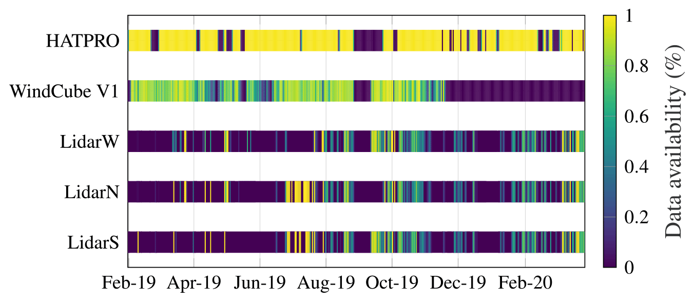
Figure 11 Daily data availability of every sensor deployed at Obrestad Lighthouse from February 2019 to April 2020. Data are shown as available for LidarS, LidarN and LidarW when the scanning beams were aligned with the wind direction recorded 100 m a.s.l.

Table 2 Scanning lidar data availability from 1 February 2019 to 29 March 2020.

4.2 Validation of the coherence estimates by sonic anemometers

This section provides an overview of the sonic anemometer data in terms of mean wind speed, mean wind direction and angle of attack (AoA). The AoA is defined here as the angle between the wind vector and the horizontal. A further study will use these sonic anemometer records to assess whether the lateral coherence of turbulence is captured properly by the long-range lidar instruments. Since the anemometers were mounted on the top of the two hydraulic masts in hilly terrain, the sectors permitting a comparison between the lidar and anemometer data need to be identified first.

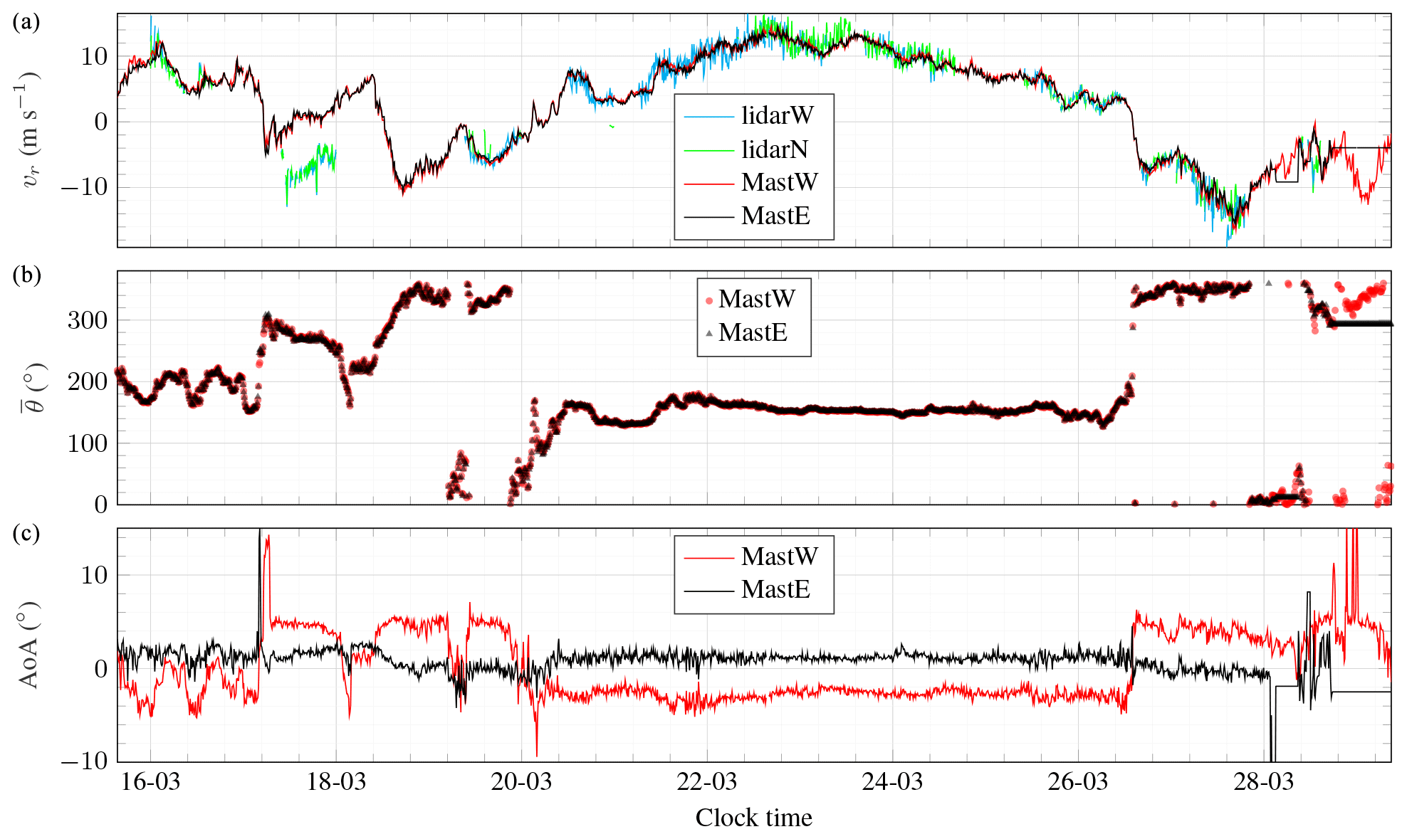
Figure 12 10 min along-beam mean wind speed (a), mean wind direction $\stackrel{\mathrm{‾}}{\mathit{\theta }}$ (b) and mean angle of attack (AoA, c) recorded from 16 to 29 March 2020 on the northern side of Obrestad Lighthouse.

Figure 12 summarizes the wind conditions recorded from 16 to 29 March 2020 by the sonic anemometers. During this period, the scanning beams of LidarW and LidarN were orientated toward the masts. The top panel of Fig. 12 displays the 10 min averaged mean wind velocity vector projected onto the scanning beam of the lidars to allow a direct comparison between the different instruments. For a southern flow, the masts are located downstream of the hill on which the lidars are installed, which is reflected by the negative AoA for MastW in the bottom panel of Fig. 12. However, the anemometer on MastE is located further away from the hill than the anemometer on MastW, which results in AoAs that differs by ca. 5^∘ between the two sensors.

The middle panel of Fig. 12 indicates that the positive AoAs observed on MastW are linked to a northerly flow, whereas the negative AoAs are associated with a wind direction around 160^∘, i.e. a southeastern flow. Even if the two masts are located only 20 m apart from each other, the flow characteristics between the two masts differ clearly due to the hilly terrain. On the top panel of Fig. 12, the wind velocity fluctuations measured with the lidar instruments are larger than by the sonic anemometers. This indicates that the flow may not be spatially uniform around the masts for a southern flow. Flow heterogeneity within small spatial separations implies that the aerosol motion inside the probe volume of the lidar is also heterogeneous. This can result in a broadening of the Doppler spectra and, therefore, a reduced measurement accuracy (Cheynet et al., 2017a). The lidar data are noisier for the southern flow than the northern one, which may be due to the presence of flow separation downstream of the hill. Therefore, the expected comparison of the co-coherence estimates from lidar and sonic measurements will have to be conducted separately for the two main wind sectors identified.

4.3 Case study

The potential of the data set collected is illustrated using a 50 min time series corresponding to a flow from southwest recorded on 25 October 2019 from 13:35 UTC (all times in this paper are UTC) with a mean wind direction of 225^∘. At the height of 80 m a.s.l., $\mathit{\zeta }=-\mathrm{0.07}$, implying near-neutral conditions on the unstable side. This particular time series was chosen for two reasons: firstly, it corresponded to a mean wind direction almost perpendicular to the coastline, such that the shore had a limited influence on the flow characteristics. Secondly, it was associated with a relatively stationary record, a mean wind speed above 13 m s⁻¹ at a height of 100 m a.s.l. and low measurement noise. At 13:30, the azimuth of the lidars was also 225^∘, indicating proper communication between the WindCube V1 and the scanning instruments. The elevation angle was 4.9^∘ such that for a scanning distance of 2 km, the measurement height was almost 200 m a.s.l. Between 13:30 and 14:20, the WindCube V1 recorded a mean wind direction of 231^∘ at 100 m above the ground, such that the mean wind direction above the wind profiler increased by only 6^∘ in 50 min. During the same period, the NORA3 hindcast provided a wind direction of 237^∘ at 100 m above the sea surface, 3 km west of the lighthouse. The small difference supports the idea that, for the case at hand, the mean wind direction did not significantly change as the flow moved toward the coast.

For hourly wind records in 2019 and 2020 with $\stackrel{\mathrm{‾}}{u}\ge \mathrm{5}$ m s⁻¹ at 10 m above ground near LidarN, the interquartile range of the wind direction difference between the NORA3 hindcast and the data collected on the mast operated by the Norwegian Meteorological Institute was only 12^∘. Therefore, it was concluded that during the COTUR campaign, the NORA3 hindcast could provide a reliable estimate of the hourly mean wind direction, especially under strong wind conditions where the error was significantly reduced.

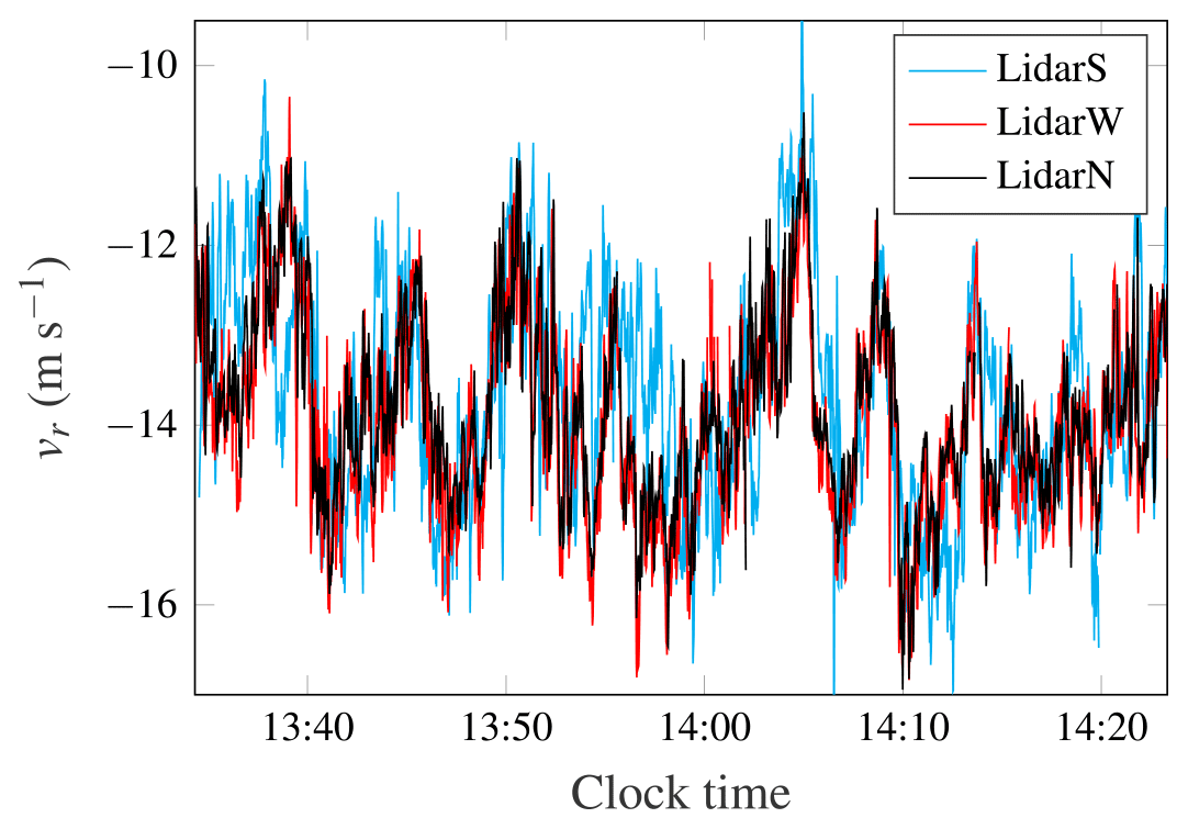
Figure 13 Along-beam velocity component recorded on 25 October 2019 by LidarN, LidarS and LidarW at r=1975 m.

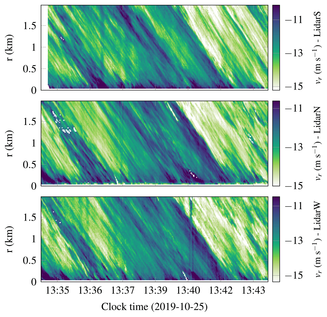
Figure 14 Along-beam velocity component simultaneously recorded on 25 October 2019 by the three scanning lidar instruments at every range gate.

The velocity fluctuations of the along-beam component, at r=1975 m from LidarN, LidarW and LidarS, are shown in Fig. 13. If the time series are visualized simultaneously for every range gate, a two-dimensional picture is obtained (Fig. 14), which is similar to a Hovmöller diagram, except that the y axis represents the distance from each lidar and the x axis represents the time. In Fig. 14, vertical stripes possibly related to electromagnetic noise (Lange et al., 2017) were filtered out using the following procedure: first, the spatially averaged along-beam wind speed was subtracted from the 2D flow field and smoothed in the time domain using a moving mean function with a 10 s window. The time-smoothed spatially averaged wind speed was then added to the flow field. This method provided satisfying results with minimal distortion of the data.

Figure 13 suggests a high spatial correlation between the velocity records by LidarN and LidarW but not between LidarS and the other two scanning instruments. Although the data quality from LidarS seems good at first sight (Fig. 14), its beam was likely misaligned with the other ones. Therefore, it was decided to assess the azimuth and elevation offsets of LidarN and LidarS with respect to LidarW.

To quantify the possible misalignments between the scanning beams, a two-step approach was used. Firstly, azimuth offsets were assessed using the correlation coefficient between measurements of two lidars using adjacent range gates. In Fig. 15, the pairs LidarW–LidarS and LidarN–LidarS show range-dependent correlation coefficients characterized by a sharp peak. The maximal value indicates where the beams are intersecting. In Fig. 15, the intersection occurs at r≈450 m and r≈550 m for the pairs LidarW–LidarS and LidarN–LidarS, respectively. The first intersection was found to be associated with an azimuth offset of 6.3^∘ for LidarS. Knowing the azimuth offset for LidarS, the one from LidarN was estimated using a similar approach, and an azimuth offset of $-\mathrm{0.4}{}^{\circ }$ was found.

Secondly, after the azimuth offsets are corrected, the elevation offsets were estimated by minimizing the root mean square error (RMSE) between the reference mean wind speed profile from LidarW and one of the other Lidars. This correction assumes that the mean flow is homogeneous in the horizontal plane between the scanning beams, which is likely the case in the MABL at separation distances lower than 100 m. Preliminary tests with noisy logarithmic profiles indicated that the elevation offset can be estimated within $\pm \mathrm{0.1}{}^{\circ }$ with this method. In these tests, a Gaussian white noise with a standard deviation of 0.03 m s⁻¹ was used, to account for the fact that the WindCube 100S has a measurement accuracy of ±0.1 m s⁻¹. The second step led to elevation offsets of −1.4 and $-\mathrm{0.4}{}^{\circ }$ for LidarN and LidarS, respectively. Since the azimuth and elevation offsets are relative to a reference sensor, which is here LidarW, the latter is associated with zero offsets. In the following, the misalignment of the beams is accounted for in the study of the coherence only.

The large azimuth offset for LidarS implies that there exist large uncertainties for the velocity records collected by this instrument compared to the other two ones. For this reason, only the co-coherence between LidarN and LidarW is studied in the following.

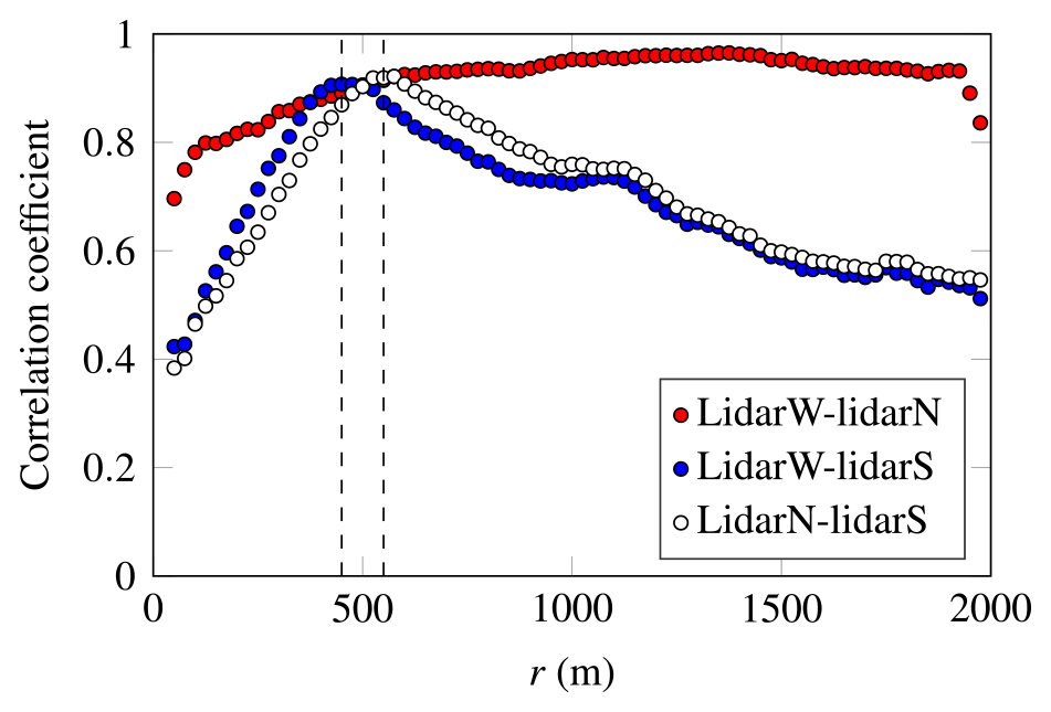
Figure 15 Pearson correlation coefficient between each pair of time series, at increasing distances from LidarW or LidarN. The dashed lines indicate the distance at which the correlation coefficient is largest for LidarW–LidarS and LidarN–LidarS.

4.3.1 Slant profiles

A slant profile is defined herein as a profile of the mean value or standard deviation of the along-beam component using scanning beams with a non-zero elevation angle. Therefore, the measurement volumes at increasing heights are obtained at increasing scanning distances. In an idealized homogeneous terrain, the slant profile would be identical to a traditional vertical profile. In the present case, the influence of the coastline on the measurement volumes decreases with the scanning distance.

Figure 16 (a, b, c) Mean wind speed recorded along the beams of the scanning lidar units (scatter) superposed to the wind profile of the WindCube V1 and the NORA3 hindcast 3 km away from the coast (solid lines). (d, e, f) Standard deviation of the along-beam component at increasing distances and heights on 25 October 2019 from 13:35 to 14:25.

The slant profiles of the along-beam mean wind speed and the along-beam standard deviations are displayed in Fig. 16. The mean wind speed profile calculated using the WindCube V1 is shown as a solid line and superposed with the slant profiles from the scanning instruments. The mean wind speed profile based on the NORA3 hindcast data collected above the sea, 3 km west of the lighthouse, is also included. This profile was first interpolated in time to overlap with the 50 min of records from 13:35 to 14:25. Then, the so-called Deaves and Harris wind speed profile (Deaves and Harris, 1982; ESDU, 2001) was used to smooth the profile along the vertical axis.

The discrepancies between the mean wind speed recorded by the scanning lidars and the wind profiler may be due to a “coastline induction zone”, which is defined here as the region upstream to the shore where the transition from sea to land induces a noticeable deceleration of the flow velocity. The profiles obtained by the scanning lidars show a strong shear at scanning distances up to 1000 m, which correspond to heights of 113 m a.s.l. The large shear suggests that the influence of the coastline on the flow characteristics could be detectable up to 1 km away from the coast. Another example of a coastal induction zone can be found in Cheynet et al. (2017b, Fig. 17). As the measurement altitude increases with the distance to the shore, the influence of the coastline on the profiles is reduced. For the heights considered, the directional wind turning is not large enough to significantly affect the profiles of the mean wind speed, especially under convective conditions where wind veering is fairly small (Brown et al., 2005; Bodini et al., 2019).

The vertical profile of the standard deviation at heights above 100 m a.s.l. shows fluctuations that are mainly due to measurement uncertainties. For LidarW and LidarN, ${\mathit{\sigma }}_{v_r}$ is almost constant between 100 and 200 m a.s.l., with variations below 0.04 m s⁻¹. The invariability of σ_u with height is expected under slightly convective conditions (Panofsky et al., 1977). Records from LidarS show stronger variations than for the other two instruments, where ${\mathit{\sigma }}_{v_r}$ increases slightly with the altitude, which is partly due to the misalignment between the laser beam and the mean wind direction.

The scanning lidars measured a turbulence intensity of 0.08 at 100 m a.s.l., which is probably slightly lower than in reality due to the probe averaging volume, which for the case at hand, filters out velocity fluctuations above 0.24 Hz (Fig. 19). Nevertheless, this value is fairly close to the one used by e.g. the IEC standard (IEC 61400-3, 2005), documented offshore (Geernaert et al., 1987; Barthelmie et al., 1996) or near offshore (Andersen and Løvseth, 2006). Some studies report also average turbulence intensities lower than in the present case, e.g. Coelingh et al. (1992) or Türk and Emeis (2010), maybe because cup anemometers were used instead of sonic anemometers.

4.3.2 Co-coherence estimates

The co-coherence is estimated as a function of the scanning distance r considering the two range gates associated with the lowest vertical separation distance. Figure 17 shows that the Davenport decay coefficients C_x and C_y increase slightly with the scanning distance, which may be attributed to the limited pointing accuracy of the instruments, as predicted in Sect. 3.4. Besides, the co-coherence can increase with height as the surface blocks the flow and distorts eddies (Kanda and Royles, 1978; Bowen et al., 1983; Cheynet, 2018). A decrease in the co-coherence with the scanning distance is also possible because the CNR reduces as r increases, which may be related to the presence of uncorrelated noise in the velocity records. Any change in the environmental conditions, including local variations of the wind direction, can affect the co-coherence estimates. The ability of long-range lidars to describe properly the co-coherence of turbulence relies on a rigorous comparison with data from sonic anemometers on met masts. As highlighted by Sect. 4.2, the instrumental setup of the COTUR campaign allows such a validation study.

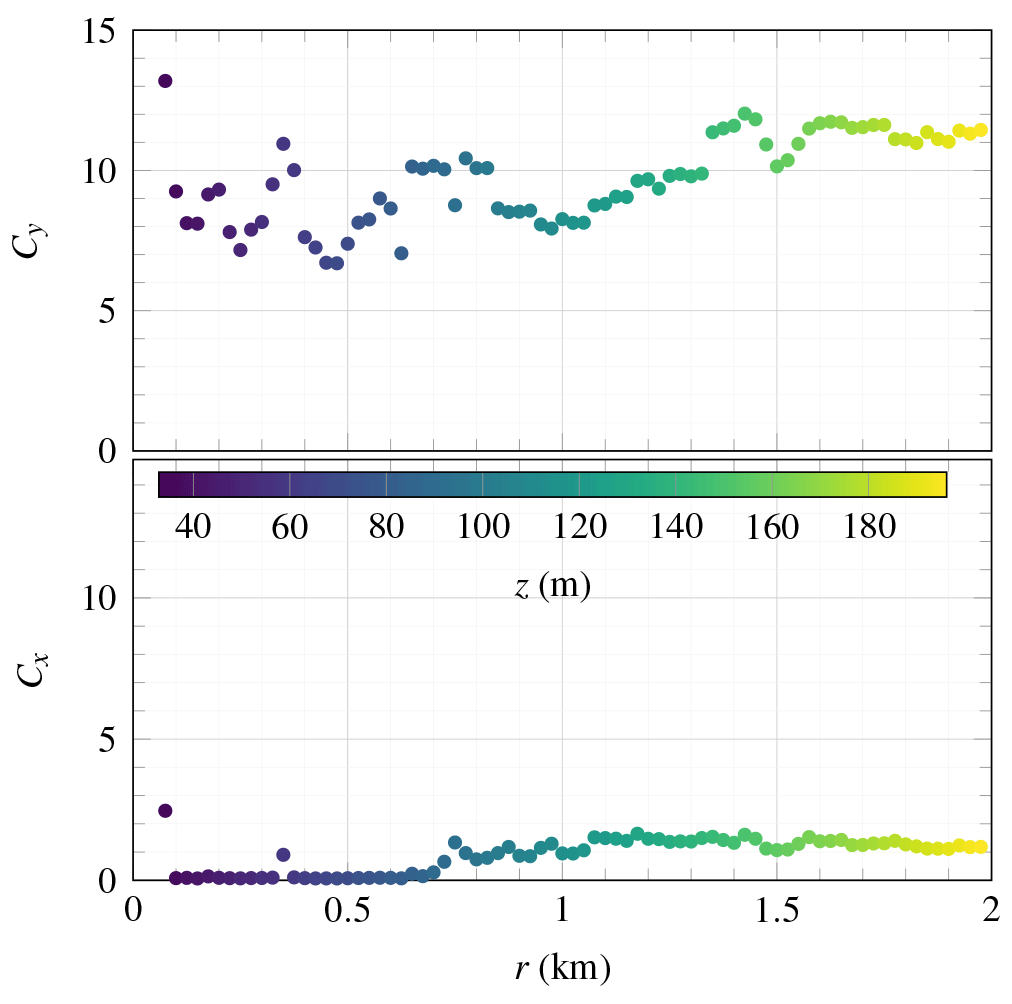
Figure 17 Decay parameters at increasing scanning distances (abscissa) and increasing heights (colour bar) obtained by fitting Eq. (7) to the co-coherence between LidarW and LidarN after correction for elevation and azimuth offsets.

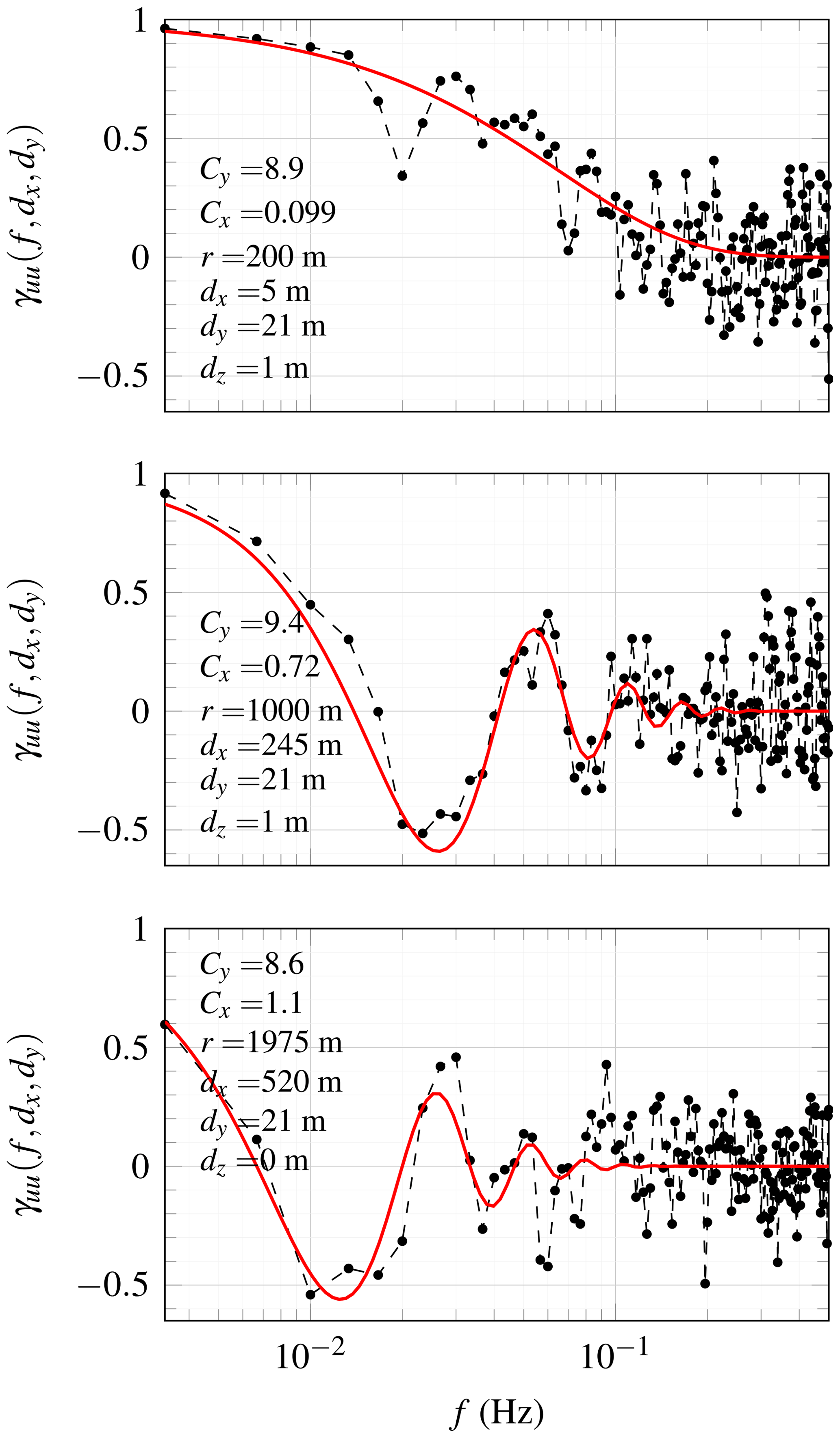
Figure 18 Estimated (scatter) and fitted (solid line) co-coherence of the along-wind component between LidarW and LidarN using range gates at 500, 1000 and 1975 m from LidarW. The time series selected is displayed in Fig. 13 and corresponds to an original azimuth of 225^∘ and an elevation of 4.9^∘, which were then corrected for possible offsets as described in Sect. 3.4.

A more detailed analysis of the lateral co-coherence between LidarN and LidarW is shown in Fig. 18 for three different scanning distances. The solid line is obtained after least-squares fitting of Eq. (7) to the data at the different range gates. As the scanning distance increases, ranges gates associated with the smallest vertical separations are located at increasingly large along-wind distance d_x (Fig. 18). A sensitivity study of the decay coefficient on the azimuth offset was conducted for LidarN with an offset ranging from −1 and 1^∘. The median value of the decay coefficient C_y ranged from 8 to 11. It was found that when d_x≫d_y, azimuth offsets had a limited impact on the estimated decay coefficients, which may explain the relatively smooth variations of C_y with r in Fig. 17.

It should be noted that a single DWL can be used to study the longitudinal co-coherence (Sjöholm et al., 2010; Davoust and von Terzi, 2016; Cheynet et al., 2017b; Debnath et al., 2020; Chen et al., 2021). In the present study, such an investigation can be conducted when the elevation angle is 2^∘, such that d_z≪d_x. The value of the C_x identified for each lidar as a function of the range gate can provide additional information on the influence of the coastline on the flow characteristics but also the existence of possible azimuth and elevation offsets.

4.3.3 Power spectral density of the along-beam velocity component

To model the dynamic wind load on a structure, knowledge of the PSDs of the velocity fluctuations is also essential. In wind engineering, the parametrization of the turbulent loading relies widely on Monin–Obukhov similarity theory (MOST) (Monin and Obukhov, 1954), which was developed for the atmospheric surface layer and mainly validated against measurements under homogeneous conditions over land (e.g. Haugen et al., 1971; Kaimal et al., 1976). The straightforward applicability of MOST for the large rotor diameters in offshore conditions is thus, at least, questionable.

The PSD of the along-beam velocity component was studied at different scanning distances and altitudes ranging from 50 to 200 m above the sea surface. In Fig. 19, only the velocity records from LidarW are selected for the sake of simplicity. A blunt spectral model (Olesen et al., 1984) was fitted to the velocity spectra at z=75 m to highlight the frequency range affected by the probe volume averaging, which is visible above 0.24 Hz.

Figure 19 Power spectral density estimate of the velocity component v_r recorded on 25 October 2019 from 13:35 to 14:25 using beams parallel to the mean wind direction with an elevation angle of 4.9^∘. The mean wind speed was $\stackrel{\mathrm{‾}}{v_r}\approx \mathrm{14}$ m s⁻¹ at the different heights selected and z_i=1153 m.

The PSD estimate is obtained using Thomson's multitaper method with a time-bandwidth product equal to $\mathrm{5}/\mathrm{2}$ (Thomson, 1982). The latter method was found to be more appropriate than Welch's algorithm (Welch, 1967) to estimate the PSD of a single time series. In Fig. 19, the different PSD estimates at z=75 m a.s.l. and above seem to be independent of the measurement height. This is not consistent with the surface-layer theory, predicting that a clear dependence of the velocity spectra on the measurement height z should be observed at z<0.1z_i, at least in the inertial subrange. The boundary layer height, assumed identical to the inversion height z_i, was 1153 m according to the passive microwave radiometer. The lack of dependence of the velocity spectrum on the height may indicate that the measurements are conducted in the mixing layer. Following Kaimal (1978, Eq. 4), the spectral peak should occur near $f{z}_i/\stackrel{\mathrm{‾}}{u}\approx \mathrm{0.65}$, but in the present case, assuming that $\stackrel{\mathrm{‾}}{v_r}\approx \stackrel{\mathrm{‾}}{u}$, it is reached at f≈0.003 Hz, i.e. at $f{z}_i/\stackrel{\mathrm{‾}}{u}\approx \mathrm{0.3}$. The spectral gap is also visible, at frequencies below 1 mHz, which is expected for near-neutral conditions (Gjerstad et al., 1995). It should be noted that the assumption $\stackrel{\mathrm{‾}}{v_r}\approx \stackrel{\mathrm{‾}}{u}$ can be challenged if the misalignment between the scanning beam and the mean wind direction is large. Nevertheless, the influence of the vertical mean wind speed $\stackrel{\mathrm{‾}}{w}$ on $\stackrel{\mathrm{‾}}{v_r}$ is likely negligible as the elevation angle is under 6^∘ (Cheynet et al., 2016b) but also because the study does not focus on weak wind conditions ($\stackrel{\mathrm{‾}}{u}<\mathrm{5}$ m s⁻¹) which are of limited relevance for wind energy application.

It should be noted that in IEC 61400-1 (2005, Eq. 5), the velocity wind spectrum becomes independent on the height at z>60 m, which is consistent with the velocity spectra displayed in Fig. 19. The preliminary results highlighted in Fig. 19 justify, therefore, the need to analyse more systematically the one-point velocity spectra recorded at heights between 50 and 200 m a.s.l.) to assess the limit of turbulence models used in codes and standards for the design of offshore wind turbines.

5 Conclusions

The data collected during the COTUR campaign aimed to characterize offshore wind turbulence, especially the lateral co-coherence, using remote sensing instruments located on the seaside. The novelty of the campaign lies in the combination of a passive microwave radiometer, three scanning Doppler wind lidars (DWLs) and one DWL profiler to explore flow characteristics not easily measurable using traditional anemometry. The lateral co-coherence was studied using synchronized lidars in a fixed line-of-sight (LOS) scanning mode with scanning beams parallel to the mean wind direction. This approach might be used to complement data collected by linear arrays of masts instrumented with sonic anemometers.

The lateral co-coherence of natural wind is significantly different from zero at low frequencies only. Therefore, it may be investigated successfully using synchronized pulsed Doppler in a similar setup as for the COTUR campaign, i.e. parallel scanning beams oriented into the mean wind direction, a probe volume of 25 m and a sampling frequency of 1 Hz. For the case at hand, the influence of the coastline on the turbulent flow characteristics may be detected up to at least 1 km away from the shore. This influence was visible in the profiles of the mean wind speed and standard deviation of the along-beam velocity component.

The combination of the LidarPlanner software with the WindScanner for turbulence characterization is another novel aspect of the study. A major step towards better availability from complex lidar scanning scenarios will be to improve the robustness of the research software tools or integration of the features into the commercial lidar software.

The data set collected during the COTUR campaign offers the possibility to cover several topics of interest for both boundary layer micro-meteorology, wind energy, remote sensing and wind engineering.

1. The comparison of the lateral co-coherence estimated by sonic anemometers and the Wind lidars offers a unique occasion to validate the potential of long-range lidar instruments to characterize the co-coherence of natural wind.

2. The decay coefficients used to model the co-coherence displayed a dependence on the scanning distance, which is partly attributed to the limited pointing accuracy of the long-range WindScanner system. As pointed out by Vasiljević et al. (2016), achieving an averaged pointing error as low as 0.01^∘ may be achievable in a near future and could become necessary to study the lateral co-coherence of turbulence at scanning distance beyond 2 km. The uncertainties associated with the pointing error suggest that the average Davenport decay coefficient for the lateral coherence studied in Sect. 4.3 is 10±2, where ± encompasses the 10–90 percentile range.

3. The use of small positive elevation angles allows the investigation of turbulence characteristics at an increasing height from the surface. While the atmospheric stability can be estimated by combining the sea-surface temperature and the data collected by the HATPRO radiometer, the latter provides also estimates of the atmospheric boundary layer height. Therefore, the limits of surface-layer scaling in the MABL can be assessed.

Remote sensing measurement of atmospheric flow above the ocean from sensors located on the seaside can be valuable to the design of the next generation of wind turbines. However, these are also deployed at increasing distances from the coast. Therefore, a detailed study of the influence of the coastline on the measured wind turbulent characteristics is required to know whether the data collected during the COTUR campaign can be directly applied to model far offshore wind conditions.