the Creative Commons Attribution 4.0 License.
the Creative Commons Attribution 4.0 License.
 | 08 Oct 2021
GFIT3: a full physics retrieval algorithm for remote sensing of greenhouse gases in the presence of aerosols
Zhao-Cheng Zeng
Vijay Natraj
Feng Xu
Sihe Chen
Fang-Ying Gong
Thomas J. Pongetti
Keeyoon Sung
Geoffrey Toon
Stanley P. Sander
Yuk L. Yung
Remote sensing of greenhouse gases (GHGs) in cities, where high GHG emissions are typically associated with heavy aerosol loading, is challenging due to retrieval uncertainties caused by the imperfect characterization of scattering by aerosols. We investigate this problem by developing GFIT3, a full physics algorithm to retrieve GHGs (CO2 and CH4) by accounting for aerosol scattering effects in polluted urban atmospheres. In particular, the algorithm includes coarse- (including sea salt and dust) and fine- (including organic carbon, black carbon, and sulfate) mode aerosols in the radiative transfer model. The performance of GFIT3 is assessed using high-spectral-resolution observations over the Los Angeles (LA) megacity made by the California Laboratory for Atmospheric Remote Sensing Fourier transform spectrometer (CLARS-FTS). CLARS-FTS is located on Mt. Wilson, California, at 1.67 km a.s.l. overlooking the LA Basin, and it makes observations of reflected sunlight in the near-infrared spectral range. The first set of evaluations are performed by conducting retrieval experiments using synthetic spectra. We find that errors in the retrievals of column-averaged dry air mole fractions of CO2 (XCO2) and CH4 (XCH4) due to uncertainties in the aerosol optical properties and atmospheric a priori profiles are less than 1 % on average. This indicates that atmospheric scattering does not induce a large bias in the retrievals when the aerosols are properly characterized. The methodology is then further evaluated by comparing GHG retrievals using GFIT3 with those obtained from the CLARS-GFIT algorithm (used for currently operational CLARS retrievals) that does not account for aerosol scattering. We find a significant correlation between retrieval bias and aerosol optical depth (AOD). A comparison of GFIT3 AOD retrievals with collocated ground-based observations from AErosol RObotic NETwork (AERONET) shows that the developed algorithm produces very accurate results, with biases in AOD estimates of about 0.02. Finally, we assess the uncertainty in the widely used tracer–tracer ratio method to obtain CH4 emissions based on CO2 emissions and find that using the ratio effectively cancels out biases due to aerosol scattering. Overall, this study of applying GFIT3 to CLARS-FTS observations improves our understanding of the impact of aerosol scattering on the remote sensing of GHGs in polluted urban atmospheric environments. GHG retrievals from CLARS-FTS are potentially complementary to existing ground-based and spaceborne observations to monitor anthropogenic GHG fluxes in megacities.
- Article
(17009 KB) - Full-text XML
- BibTeX
- EndNote


Remote sensing of greenhouse gases (GHGs) in cities provides abundant datasets for quantifying urban carbon sources and sinks, complementary to in situ ground-based measurements. However, large source regions such as megacities are also typically associated with heavy aerosol loading. Atmospheric aerosols modify the path of solar radiation and thereby introduce uncertainties in the retrieval of GHGs from reflected and scattered sunlight measurements. It has been suggested that the imperfect characterization of aerosol optical and microphysical properties is a significant source of error for GHG retrievals (Butz et al., 2009; O'Dell et al., 2011). Many different full physics retrieval algorithms, which explicitly account for atmospheric absorption and scattering and surface reflection in the radiative transfer (RT) forward modeling, have been developed for spaceborne instruments for retrieving column-averaged dry air mole fractions of atmospheric carbon dioxide (XCO2) and methane (XCH4). Examples of these instruments include Orbiting Carbon Observatory-2 (OCO-2; Boesch et al., 2011; O'Dell et al., 2018; Reuter et al., 2017), the Greenhouse gases Observing SATellite (GOSAT; Bril et al., 2012; Butz et al., 2011; Yoshida et al., 2013), and TanSat (Wang et al., 2020; Yang et al., 2020). Full physics algorithms for retrieving GHGs explicitly fit aerosol optical and microphysical properties in order to minimize biases induced by scattering. Although the GHG retrievals show good agreement with ground-based Total Carbon Column Observing Network (TCCON) results, the retrieved aerosol optical depth (AOD) values have large differences compared with collocated AErosol RObotic NETwork (AERONET) measurements (Nelson et al., 2016) probably due to limited information content for aerosols and interference from other factors. To minimize data uncertainty, many operational GHG retrieval algorithms filter out retrievals with optically thick aerosols. Observations from these spaceborne instruments are made in side scattering directions (scattering angles between ∼90 and 150∘), where aerosol scattering effects are greatly reduced compared to the forward scattering direction. However, for an observatory targeting urban GHGs from other vantage points, such as the California Laboratory for Atmospheric Remote Sensing Fourier transform spectrometer (CLARS-FTS) (Fu et al., 2014), which is located on the top of Mt. Wilson overlooking the Los Angeles (LA) Basin, the measurements are made in both backscattering and forward scattering directions (Zeng et al., 2020a). There has been very little prior work investigating impacts of aerosol scattering on GHG retrievals for a wide range of viewing geometries.
The main objective of this study is to demonstrate the performance of a full physics algorithm (hereafter referred to as GFIT3), which is an extension of the widely used GFIT model, to retrieve GHGs in polluted urban atmospheres from spectra of reflected solar radiation. GFIT is a state-of-the-art profile scaling algorithm to retrieve gas concentrations and related atmospheric and instrumental parameters from absorption spectra. It has been the primary retrieval algorithm for the TCCON network (Wunch et al., 2011), which has been the benchmark for validating satellite-based trace gas observations. GFIT has also been used to analyze spectra from the MkIV balloon interferometer (e.g., Sen et al., 1996) and ATMOS (e.g., Irion et al., 2002) and is also a critical component of the currently operational CLARS-GFIT retrieval algorithm (Fu et al., 2014). GFIT2 (Connor et al., 2016; Roche et al., 2021) is an upgraded version of GFIT that enables the retrieval of vertical profiles of trace gases. While GFIT scales profiles based on optimal estimation, GFIT2 uses Bayesian optimal estimation theory (Rodgers, 2000) as the inverse method to retrieve GHGs at different altitudes. However, both GFIT and GFIT2 do not account for scattering from molecules and particulates in the atmosphere. Such contributions are negligible in the near-infrared domain for instruments that measure directly transmitted solar spectra, such as TCCON. However, for GHG retrievals based on reflected solar radiation measurements (e.g., CLARS-FTS, GOSAT, and OCO-2), the aerosol scattering effect is important and needs to be accurately modeled. GFIT3 is designed specifically for the purpose of retrieving GHGs in polluted atmospheres from reflected solar radiation observations. It includes an aerosol model and a fast RT model to simulate the aerosol scattering contributions. The technical details can be found in Sect. 3.
In this study, we specifically focus on measuring GHGs in the LA megacity, which is one of the most polluted cities and the second largest contributor to carbon emissions in the US, using observations from CLARS-FTS. We investigate the impacts of aerosol scattering on GHG retrievals using GFIT3 to jointly retrieve GHGs (CO2 and CH4) and AODs of coarse- and fine-mode aerosols. CLARS-FTS observes reflected sunlight in the near-infrared spectral range. CLARS-FTS observations provide a unique dataset to study the impact of aerosol scattering effect because of (1) the large viewing zenith angle () and larger range of scattering angles compared to spaceborne instruments (Zeng et al., 2020a) and (2) the longer light path in the planetary boundary layer (PBL) that is a consequence of the large viewing zenith angle. While a longer light path increases the sensitivity of the measurements to anthropogenic emissions from LA, it also makes the measurements susceptible to light path change due to aerosol particles in the PBL (Zhang et al., 2017). As a result, any effects from aerosol scattering on GHG remote sensing become amplified for CLARS-FTS due to its observation geometry. It is therefore very important to have proper aerosol models with accurate optical properties, including phase function and single scattering albedo (SSA), in order to obtain accurate GHG retrievals.
Another scientifically unique feature of CLARS-FTS, among instruments that measure surface-reflected sunlight, is that it uses the O2 1Δ band at 1.27 µm instead of the O2 A band at 0.76 µm that is traditionally used by spaceborne instruments to constrain surface pressure and aerosols. Since the 1Δ band is closer to the CO2 and CH4 absorption bands around 1.6 µm, scattering effects in the GHG absorption bands are likely to be better constrained. Also, the spectroscopy of the 1Δ band is more accurately known than that of the A band. The 1Δ band was not selected by current spaceborne instruments because of contamination from airglow emitted by oxygen molecules in the upper atmosphere. Recently, Bertaux et al. (2020) showed that the airglow contribution can be distinguished and separated from the O2 absorption signal. Usage of the 1Δ band will be tested in the upcoming MicroCarb mission (Bertaux et al., 2020), the first such attempt for a spaceborne instrument. Since CLARS-FTS looks downwards toward the basin, the measured spectra are not affected by airglow, which originates in the upper atmosphere. Outcomes from this study will shed light on the merits of using the 1Δ band for GHG remote sensing.
The paper is organized as follows. The CLARS-FTS instrument is introduced in Sect. 2. The GFIT3 retrieval algorithm is described in Sect. 3. In Sect. 4, we demonstrate retrieval experiments using synthetic spectra to evaluate GFIT3. Retrieval results for CLARS observations are presented in Sect. 5, followed by discussions and conclusions in Sects. 6 and 7, respectively.
2.1 CLARS-FTS
CLARS-FTS was designed and built at the Jet Propulsion Laboratory. It is optimized for reflected sunlight measurements with high spectral resolution in the near-infrared region (4000–15 000 cm−1). CLARS-FTS uses a pointing system to target a set of predefined surface reflection targets (Fig. 1) in the LA Basin, as well as a local diffuse reflector (Spectralon) for measurements of the free tropospheric background (Zeng et al., 2020b). In the Los Angeles Basin Survey (LABS) operating mode, the pointing system stares at each surface reflection target in the LA Basin and records atmospheric absorption spectra using reflected sunlight as the light source. In the absence of aerosols, as shown in Fig. 1a, sunlight travels through the PBL twice with a defined path: once on the way to the surface target and a second time from the surface target to CLARS-FTS. The resulting light path through the PBL is greater than 5 km (see Table 1 in Wong et al., 2015), which is several times longer than other commonly used viewing geometries, e.g., observing the direct solar beam from the surface, or measurement of surface-reflected sunlight from aircraft and spacecraft vantage points. In the presence of aerosols, the light path changes mainly due to aerosol scattering along the path from the basin to the mountain top. Examples of single and multiple scattering are demonstrated in Fig. 1a. CLARS covers the whole basin every 1.5 to 2 h. Depending on the season, the total number of observations within a single day ranges from 160 to 260, and the number of repeated scans of the whole basin is between five to eight times over the same timeframe. Additional details can be found in Fu et al. (2014). Figure 1b shows examples of the observed radiance in the O2 absorption band centered at 7885 cm−1, the weak CO2 absorption band (hereafter referred to as WCO2) at 6220 cm−1, the CH4 absorption band at 6076 cm−1, and the strong CO2 absorption band (hereafter referred to as SCO2) at 4852 cm−1. The absolute radiance, which is needed to constrain the aerosol scattering and the surface reflectance, is derived by calibrating the raw spectral data of digital numbers. The calibration factor is derived by comparing the CLARS-FTS spectra with that of a collocated ASD spectroradiometer. The signal-to-noise ratio (SNR) for the WCO2 and CH4 bands is about 300±80; for the O2 and SCO2 bands, the SNR is about 100–150 depending on the surface target.
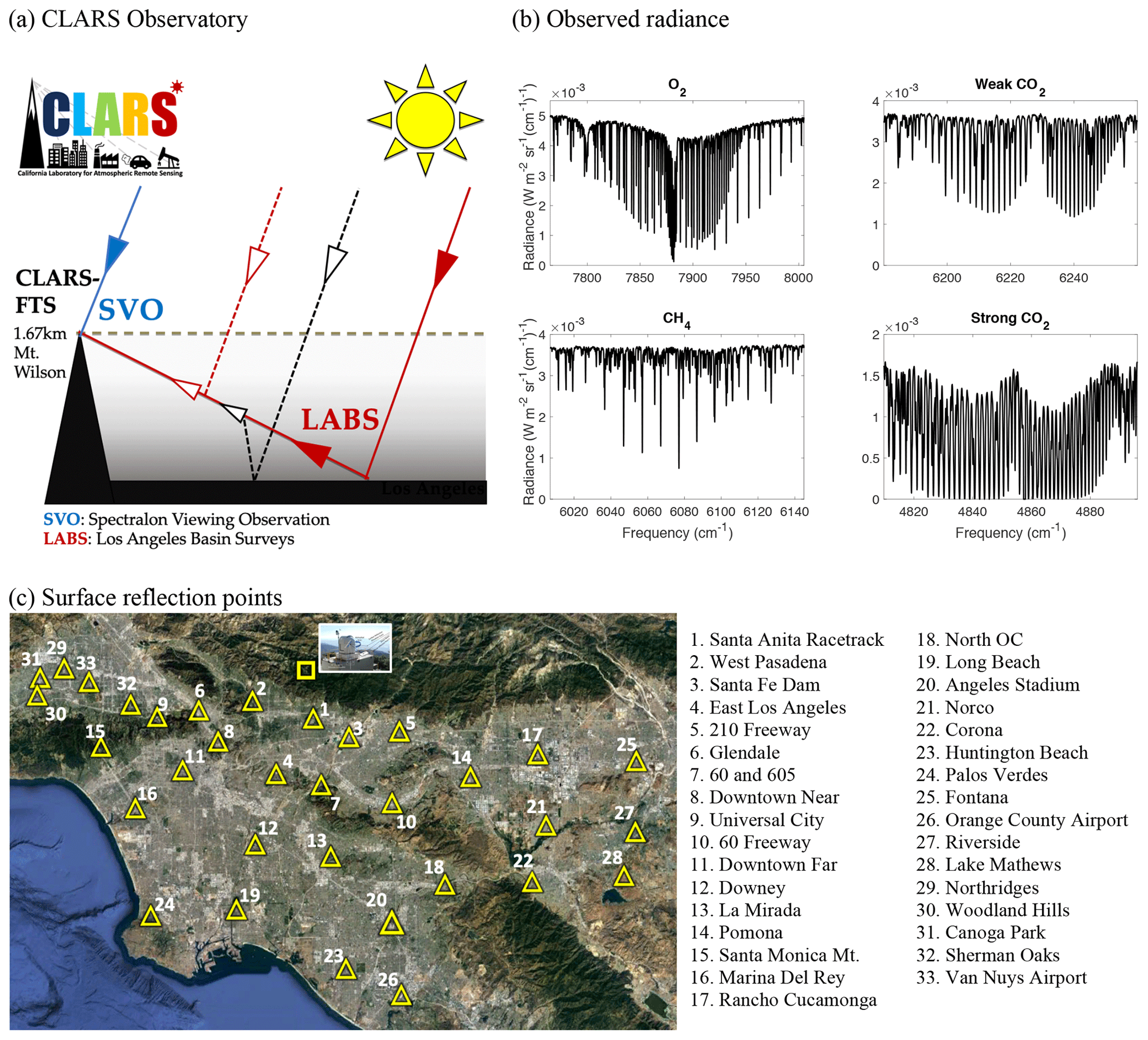
Figure 1(a) Schematic figure of the CLARS observatory. The lines depict incident and reflected sunlight from an example surface reflection target. The LABS and Spectralon viewing observation (SVO) modes are illustrated. For the LABS mode, examples of contributions from single scattering (dotted red) and multiple scattering (dotted black) are also illustrated. (b) Examples of observed high-resolution (0.06 cm−1) spectra for the O2 1Δ absorption band centered at 1.27 µm (7885 cm−1), the weak CO2 absorption band at 6220 cm−1, the CH4 absorption band at 6076 cm−1, and the strong CO2 absorption band at 4852 cm−1. These measurements were made on 28 September 2013 over the Santa Anita Racetrack surface reflection point at local noon. (c) The 33 surface reflection points across the Los Angeles Basin. The background image is adopted from © Google Earth.
2.2 Observation geometries
Compared to low earth orbiting satellites such as OCO-2/3, observations from CLARS-FTS have a larger range of aerosol scattering angles mainly due to the diurnal and seasonal change in incident solar geometry (Zeng et al., 2020c). Figure 2 shows the diurnal change in aerosol scattering angle for six selected surface reflection points. In the morning, the surface reflection points to the west (West Pasadena and Santa Monica) have large scattering angles that gradually change to smaller scattering angles in the late afternoon. The opposite pattern of change can be observed at reflection points to the east (Santa Fe dam and Rancho Cucamonga). At reflection points to the south (Santa Anita and Long Beach), the changes are smaller than at other targets. These changes are a result of the fixed viewing geometry for each surface reflection target but varying solar geometry. A detailed description of the angular scattering effect can be found in Zeng et al. (2020c). This large range of angles, from forward scattering () to backward scattering (), means that a majority of the change in aerosol scattering comes from angular variations. This also indicates that the aerosol scattering phase function is a key parameter that needs to be accurately modeled in order to obtain high-fidelity RT calculations.
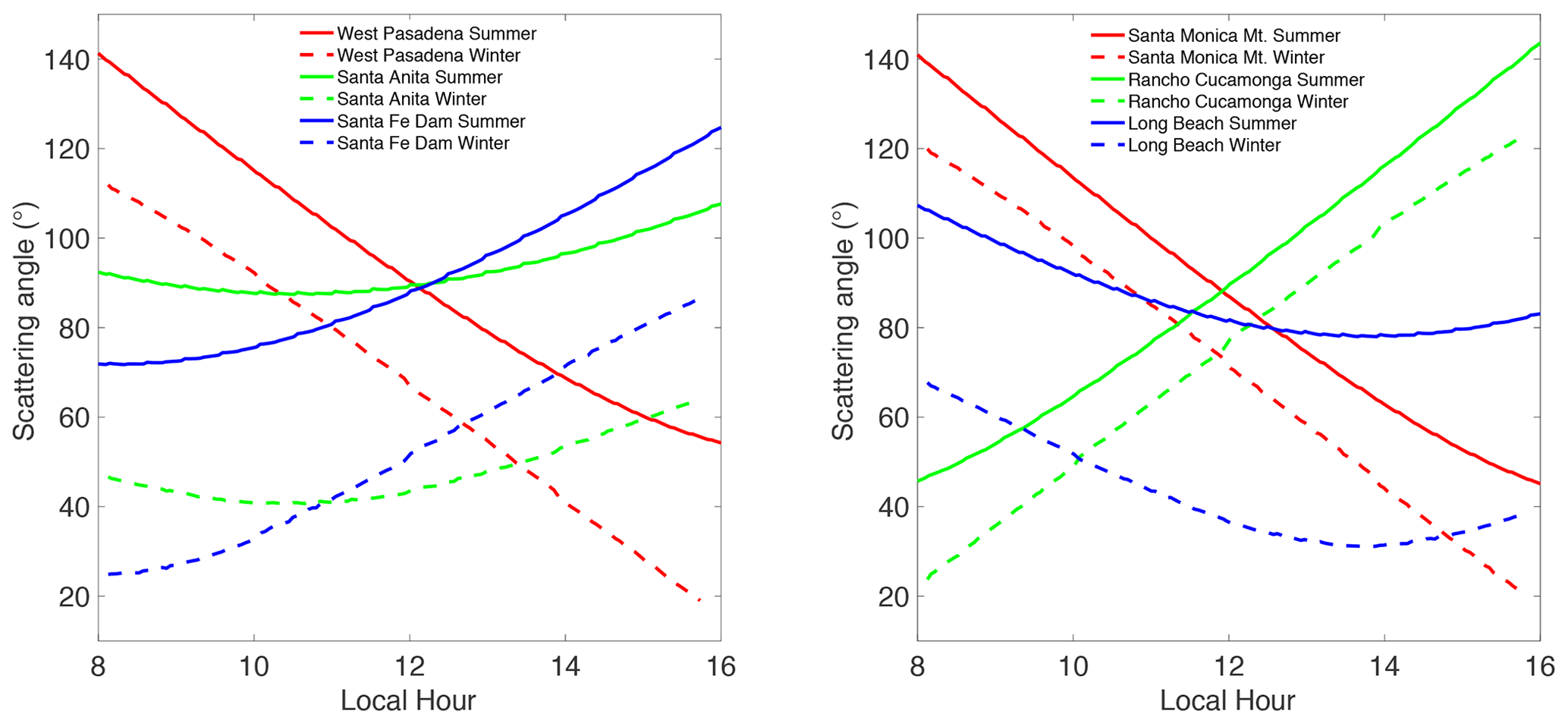
Figure 2Diurnal change in aerosol scattering angle for six selected surface reflection points, separated into two groups. Group 1 includes points #1 Santa Anita Racetrack, #2 West Pasadena, and #3 Santa Fe Dam that are close to CLARS-FTS; group 2 includes #15 Santa Monica Mt., #17 Rancho Cucamonga, and #19 Long Beach that are further away. Hourly scenarios from 20 June and 22 December 2013 are used to represent summer and winter solar geometries, respectively.
GFIT3 incorporates the following four major components: (1) a pre-processing step using the CLARS-GFIT algorithm to generate gas absorption coefficients and other related parameters, as well as the O2 slant column density (SCD) for excluding cloudy and heavy aerosol loading soundings; (2) a forward RT model (RTM) to generate synthetic spectra in order to simulate observed CLARS-FTS spectra; (3) an inverse model based on optimal estimation to update the surface and atmospheric state vector to minimize the difference between model and observation; and (4) a post-processing screening step to filter out bad retrievals. The workflow chart is shown in Fig. 3.
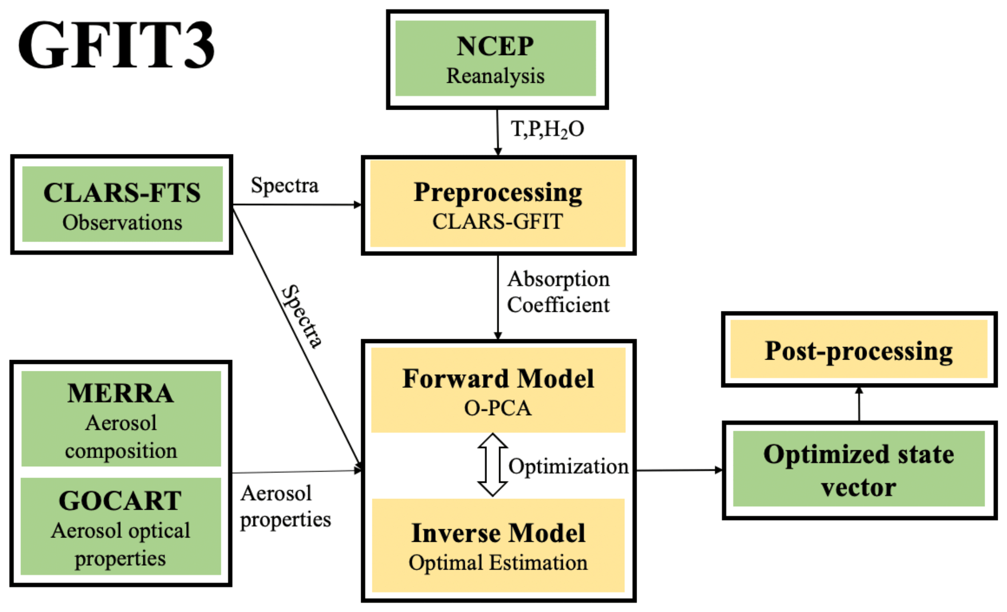
Figure 3Workflow of GFIT3 for retrieving XCO2 and XCH4 from CLARS-FTS observations. There are four major components: (1) a pre-processing step to identify soundings free of clouds and heavy aerosol loading; (2) a forward RTM to generate synthetic spectra in order to simulate observed CLARS-FTS measurements; (3) an inverse model based on optimal estimation to update the surface and atmosphere states to minimize the difference between model and observation; and (4) a post-processing screening step to filter out bad retrievals.
3.1 Pre-processing using CLARS-GFIT
The objective of pre-processing is to identify measurements that are affected by clouds and/or heavy aerosol loading and to exclude them before the full physics retrieval. We employ CLARS-GFIT (Fu et al., 2014), which is a modified version of the GFIT program (version GGG2014), to retrieve O2 SCD using the same spectral bands and spectroscopic parameters used by TCCON. The recently released GGG2020 with major updates to the spectroscopic line lists will be incorporated into CLARS-GFIT in the near future. Aerosol scattering is not considered in CLARS-GFIT; the ratio of retrieved O2 SCD to calculated O2 SCD estimated from surface pressure reanalysis data (National Center for Environmental Prediction (NCEP) reanalysis in this study), denoted by O2 ratio, acts as a proxy (Zeng et al., 2020c). We filter out data with (1) a O2 ratio less than 0.85 (low clouds and high aerosol loading) and larger than 1.02 (high clouds); (2) SNR less than 100; (3) solar zenith angle (SZA) larger than 70∘; and (4) spectral fit error larger than 1σ above the mean of all the spectral fitting residuals. The gas absorption coefficients, a priori atmospheric profiles, and solar lines processed by CLARS-GFIT will also be used in the forward RTM of GFIT3.
3.1.1 Calibrating O2 absorption cross section
Analysis of the O2 ratio under different aerosol conditions reveals a systematic bias (about 2 %) between the retrieved O2 SCD and that calculated using the NCEP reanalysis surface pressure even in situations when the atmosphere is clear (Appendix Fig. A1). Such a bias in the 1Δ band has been reported by Washenfelder et al. (2006), who found that for the TCCON spectra, the retrieved column O2 is consistently 2.27 %±0.25 % higher than the dry pressure column estimated from the surface pressure. This bias in TCCON retrievals is consistent with values for CLARS-GFIT retrievals. A similar systematic bias was found by Butz et al. (2011) for the O2 A band at 0.76 µm from satellite observations. These biases are most likely attributable to spectroscopic uncertainties. We adopt a simple method of scaling the absorption cross sections in the 1Δ band by a factor of 1.02 to make our modeled radiances in the 1Δ band consistent with observations.
3.2 Forward model
3.2.1 Optical-property-based principal component analysis RTM
RT models simulate the radiance based on inputs of the state vector and related model parameters. In theory, a sophisticated line-by-line RTM (e.g., LIDORT; Spurr, 2008) with a high number of computational quadrature angles (streams) is needed to accurately simulate the propagation of sunlight through the atmosphere. However, simulation of high-resolution CLARS-FTS spectra that require resolving gas absorption lines with fine spectral sampling is computationally expensive. Instead, many fast RTMs (e.g., Butz et al., 2011; O'Dell et al., 2012; Somkuti et al., 2017) have been developed to speed up the radiance calculation without introducing large systematic errors in the trace gas retrieval. In this study, we adopt an optical-property-based principal component analysis (O-PCA) RTM developed by Natraj et al. (2005, 2010) and improved by Kopparla et al. (2016, 2017). The O-PCA procedure was linearized and analytic Jacobians developed for the PCA-based radiation fields by Spurr et al. (2013). It has been shown to be fast and accurate for retrieving CO2 from satellite measurements (Somkuti et al., 2017). The O-PCA method first divides the spectral region into bins. Each bin is characterized by grouping certain optical properties (such as atmospheric layer trace gas optical depth values or single scattering albedos) that are similar within the bin. The selection for spectral binning is typically based on the division of (the logarithms of) the total-atmosphere gas optical depths into decadal intervals. We use 11 bins in this study. For each bin, PCA is implemented on a dataset that includes the extinction optical depth and single scattering albedo profiles, as well as the (wavelength-dependent) surface albedo and column optical depth for each aerosol type. High-accuracy line-by-line multiple scattering calculations (using LIDORT in this work) are then performed for profiles representing the bin mean and PCA-perturbed properties. For this analysis, we use 32 streams for these calculations. The multiple scattering calculations are computationally expensive; the reduction of the number of these calculations is the main reason for the speed-up afforded by O-PCA. O-PCA also performs a fast and low-accuracy line-by-line calculation of the radiances using the two-stream exact single scattering (2S-ESS; Spurr and Natraj, 2011) model for every spectral point in the band. The 2S-ESS model computes both the single scattering contribution to the radiance and a two-stream approximation to the multiple scattering contribution. Finally, the total radiance field is obtained for every point in the bin by calculating a wavelength-dependent correction factor to adjust the 2S-ESS calculations. A detailed description of the O-PCA methodology can be found in Kopparla et al. (2017) and Spurr et al. (2013). Simulations (see Fig. 4) show that, while the accuracy of O-PCA depends on the aerosol loading, almost all of the spectral calculations have an error of less than 0.1 %. The root mean square error (RMSE) is less than 0.01 %.
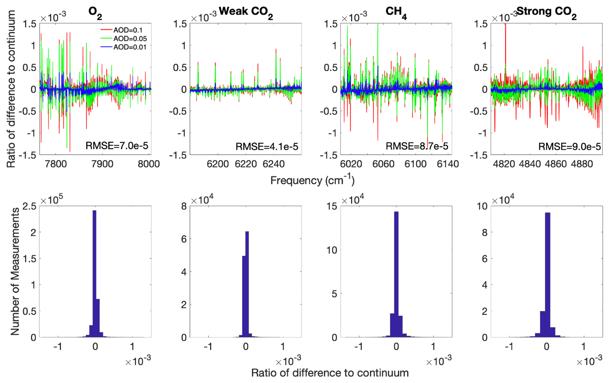
Figure 4Ratio of the difference (relative to the continuum value) between simulated radiances (using O-PCA) and high-accuracy computations (using LIDORT with 32 streams). These calculations are based on the 240 scenarios, with different observation geometries and atmospheric profiles, described in the inverse experiments in Sect. 4. Four empirical orthogonal functions are used for the O-PCA computations. Three different aerosol scenarios are considered, with AOD values of 0.01, 0.05, and 0.1 in the 1.27 µm O2 1Δ band. The overall RMSEs are also indicated.
3.2.2 State vector
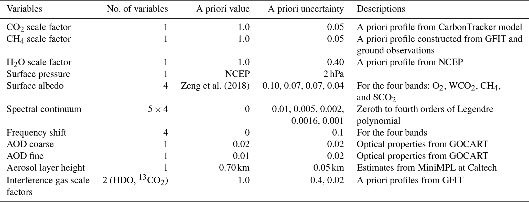
The state vector includes all variables that are to be retrieved by GFIT3 in order to fit the observed spectra. These variables are inputs to the forward RTM. Table 1 summarizes all the variables in the state vector and the values used for their uncertainties in the retrieval.
Table 1Summary of variables in the state vector and their uncertainties.
(1) CO2 and CH4 profiles
We follow the TCCON methodology and perform a retrieval that scales predefined vertical shapes of CO2 and CH4 to obtain XCO2 and XCH4. This is faster and simpler than a full profile retrieval that independently scales gas mixing ratios at different altitudes. The profile scaling method is also less sensitive to systematic errors related to the shape of the calculated spectral lines, such as instrumental line shape and spectroscopic line widths (Wunch et al., 2011). Although a profile retrieval is possible, there are not enough degrees of freedom in the measurement to fully resolve the gas profile. Therefore, the retrieval problem will be ill-posed and underdetermined if strong constraints are not imposed on the vertical profile. Sensitivity tests show that the profile scaling approach is efficient and that errors from possible bias in the profiles are small (Sect. 4).
To account for GHG enhancement in the LA PBL, we used CO2 simulations from the widely used CarbonTracker CO2 model (Peters et al., 2007), which is an assimilation model incorporating available observations. The 3-hourly simulations are available from the CarbonTracker CO2 model. Monthly averaged CO2 profiles are used as the a priori profiles in GFIT3 (Fig. 5a). For CH4, since high-resolution simulations are not available at city scale, we reconstruct the profiles based on CLARS-GFIT a priori. A constant PBL enhancement of 91 ppb (parts per billion), as estimated by Verhulst et al. (2017; Table 5) using the NASA megacity network, is added to the monthly averaged CH4 profiles, as shown in Fig. 5b. Diurnal changes in the PBL enhancement are not considered in this analysis.
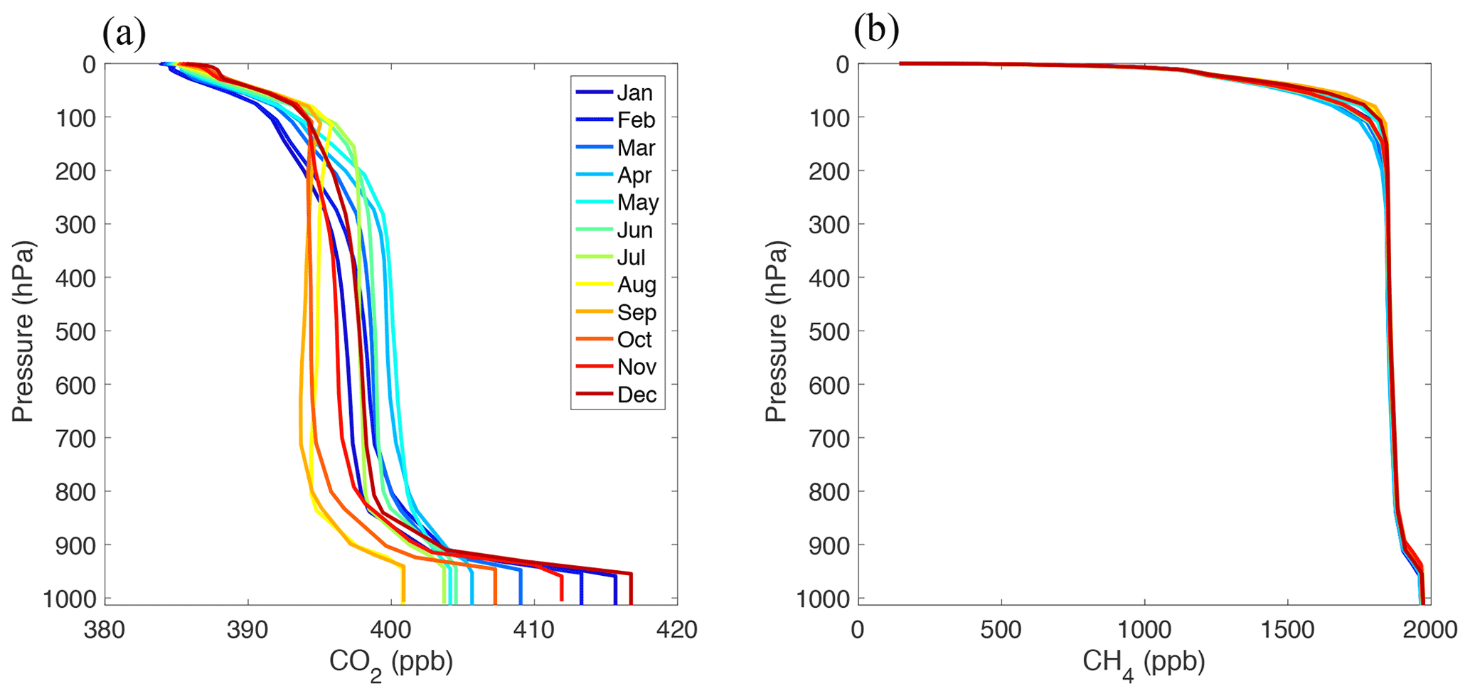
Figure 5(a) CO2 vertical profiles are extracted from the CarbonTracker model over Los Angeles with 3-hourly temporal resolution. Monthly averaged profiles are used as a priori profiles in GFIT3. (b) Monthly averaged CH4 vertical profiles are adopted from CLARS-GFIT. A constant PBL enhancement of 91 ppb, as estimated by Verhulst et al. (2017; Table 5) using the NASA Megacity network, is added. The hourly variability in CH4 in the PBL is assumed to be the same as that of CO2 since they are co-emitted and follow a similar atmospheric mixing process.
(2) Surface albedo and aerosol properties
The contributions to the observed radiance from surface reflectance and aerosol scattering are coupled. Similar to Zeng et al. (2018), we assume a Lambertian surface and calculate the a priori surface albedo by ratioing the measured radiance reflected from the surface target by that reflected by a Spectralon board beside the FTS. The Spectralon measurement represents the incident radiance before entering the PBL. For aerosols, we use AOD values from Modern Era Retrospective analysis for Research and Applications Aerosol Reanalysis (MERRAero) data (Rienecker et al., 2011) and associated optical properties from the Georgia Institute of Technology–Goddard Global Ozone Chemistry Aerosol Radiation and Transport (GOCART; Chin et al., 2002) model, which includes five aerosol types: sea salt, dust, organic carbon, black carbon, and sulfate. In light of the difficulty in resolving so many aerosol types from measurements, we separate the five aerosol types into two groups based on size: coarse-mode (sea salt and dust) and fine-mode (organic carbon, black carbon, and sulfate). While the sizes, extinction efficiency, and phase function of aerosols in the fine mode are similar, the black carbon has a much smaller single scattering albedo (SSA). For sea salt and dust aerosols, five differently sized bins are separately tracked in the Modern-Era Retrospective analysis for Research and Applications (MERRA) model. The sea salt, black carbon, organic carbon, and sulfate are all hygroscopic. GFIT3 uses monthly average aerosol optical properties (extinction efficiency, SSA, and phase function) at four daytime hours (07:00, 10:00, 13:00, 16:00 LT). The monthly averaged density fraction of aerosols is shown in Fig. 6. While the fine-mode aerosols show identical monthly variabilities, the coarse-mode particles show a clear seasonal cycle, with more sea salt in summer originating from the ocean and more dust in winter originating from the Mojave desert and transported to the LA Basin. Figure 7 shows the wavelength dependence of aerosol optical properties averaged over all months in 2013. Fine-mode aerosols have a larger Ångström exponent, and hence a greater wavelength dependence, than coarse-mode aerosols. To illustrate changes in phase function, the asymmetry factor (that quantifies the extent of forward scattering) is used. An asymmetry factor value of 0 represents isotropic scattering; the value increases to 1.0 as the phase function peak sharpens in the forward direction.
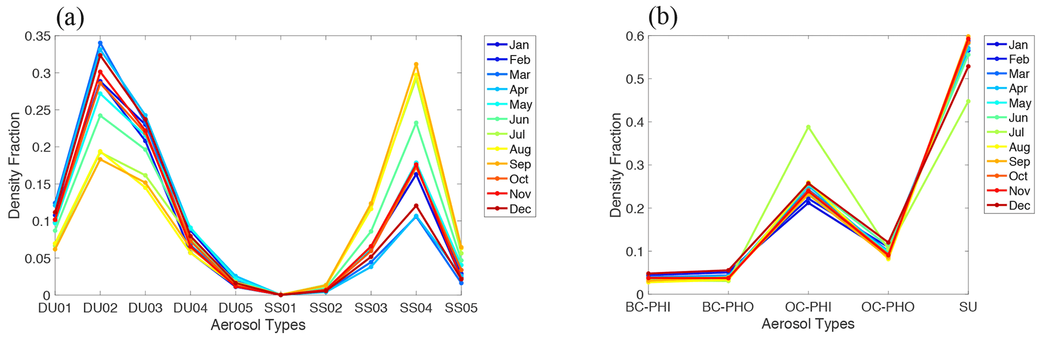
Figure 6Aerosol composition from Modern-Era Retrospective Analysis for Research and Applications (MERRA) reanalysis data for LA (07:00, 10.00, 13:00, 16:00 LT). (a) Monthly averaged density fraction of aerosols for dust and sea salt. The dry size bins for dust (DU01 to DU05) correspond to the radius limits (in microns) 0.1–1, 1–1.8, 1.8–3, 3–6, and 6–10, respectively. Similarly, for sea salt (SS01 to SS05), the corresponding values are 0.03–0.1, 0.1–0.5, 0.5–1.5, 1.5–5, and 5–10, respectively. (b) Monthly averaged density fraction for hydrophilic black carbon (BC_PHI), hydrophobic black carbon (BC_PHO), hydrophilic organic carbon (BC_PHI), hydrophobic organic carbon (BC_PHO), and sulfate (SU). MERRA data below the CLARS-FTS elevation (1.67 km) are used.
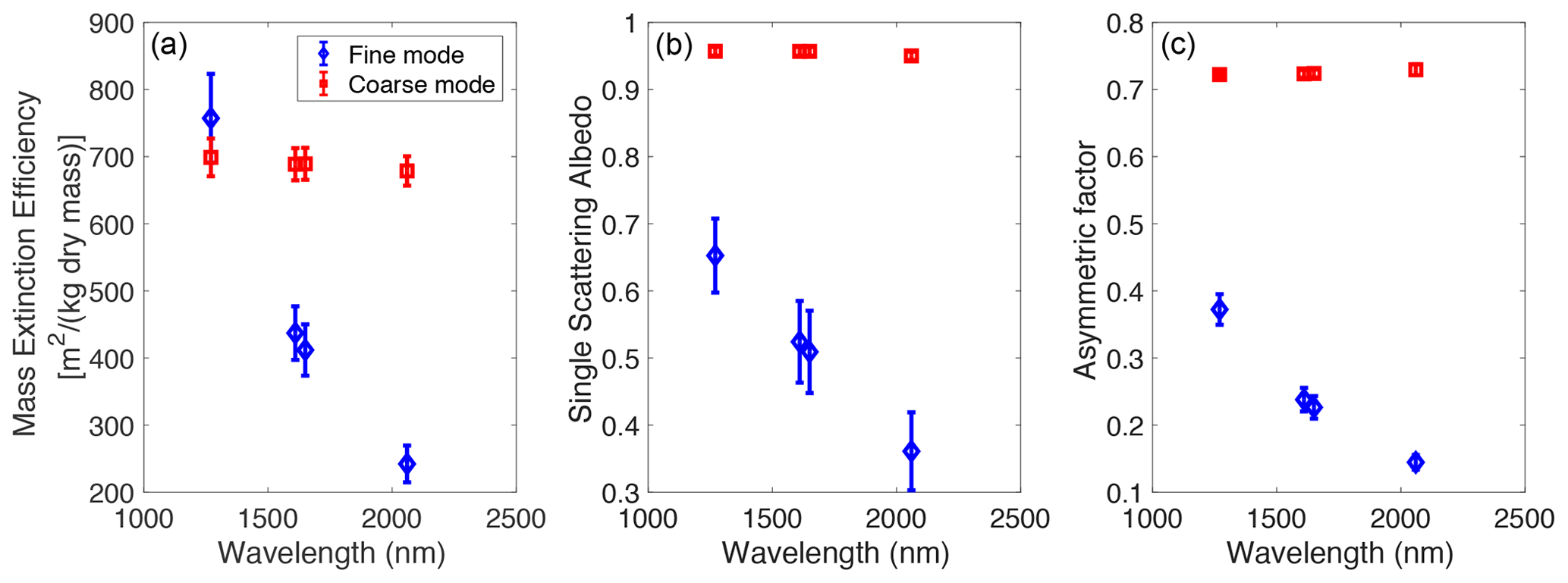
Figure 7Wavelength dependence of aerosol optical properties (averaged over a year) in the 1.27 µm O2 1Δ absorption band, 1.61 µm weak CO2 absorption band, 1.65 µm CH4 absorption band, and 2.06 µm strong CO2 absorption band from the Georgia Institute of Technology–Goddard Global Ozone Chemistry Aerosol Radiation and Transport (GOCART) model. (a) Mass extinction efficiency, (b) single scattering albedo, and (c) asymmetry factor for fine (blue) and coarse (red) modes. These aerosol optical properties are density weighted on a monthly basis for daytime only (07:00, 10:00, 13:00, 16:00 LT). For aerosols that are hygroscopic (size dependent upon relative humidity), monthly average humidity is used.
In the retrieval algorithm, we retrieve AODs for the coarse and fine modes, in addition to the aerosol layer height (ALH; Table 1). The single scattering albedos (SSAs) and phase functions of the coarse and fine modes are prescribed and not retrieved. The effective SSA for the coarse mode is calculated as the mean of the SSA values (from the GOCART model) of sea salt and dust, weighted by their simulated AODs from MERRAero. The same approach is applied to fine-mode aerosols except using black carbon, organic carbon, and sulfate. The effective phase functions can be calculated in a similar manner, except that the weighting is done by the scattering AOD. We do not consider the geometric thickness of the aerosol layer since it has a much smaller impact on the observed radiance compared to the total AOD (Zeng et al., 2019). Practically, in the forward model, the aerosols are placed in two adjacent layers. The fractions of AODs in each layer are adjusted (with total AOD conserved) to change the effective ALH. Since both fine- and coarse-mode aerosols are relatively well mixed in the atmosphere, we assume that they have the same effective ALH. The a priori AODs are derived from monthly averaged AERONET observations at Caltech and the a priori ALH from an aerosol profiling lidar (MiniMPL), also at Caltech (Zeng et al., 2018). For the retrievals, the a priori ALH is set to 0.7 km, representing an average from all available MiniMPL observations.
(3) Surface pressure
The a priori surface pressure is extracted from NCEP reanalysis data (Kalnay et al., 1996), which is used for GGG2014 TCCON retrievals (Wunch et al., 2015). A comparison with ECMWF ERA5 reanalysis (Hersbach et al., 2020), which has a higher resolution, indicates that the two surface pressure datasets are highly correlated, with a standard deviation of the difference of about 2 hPa (Zeng et al., 2020b). In the GFIT3 retrieval, we assume this value as the uncertainty for surface pressure.
3.2.3 Solar model
To construct the high-resolution solar irradiance, we combine the solar continuum level estimated from the solar spectrum developed by Kurucz (2005) (http://kurucz.harvard.edu/sun/irradiance2008/, last access: 20 September 2021) and the high-resolution solar pseudo-transmittance spectrum from GFIT (Toon, 2014; https://mark4sun.jpl.nasa.gov/toon/solar/solar_spectrum.html, last access: 20 September 2021). The Kurucz spectrum was created from the solar spectrum measured by a high-resolution FTS at the Kitt Peak National Observatory. In the near-infrared spectral regions of relevance to this work, Toon's solar pseudo-transmittance spectrum is a combination of high-resolution spectra from balloon FTS, ground-based Kitt Peak, and TCCON observations. A similar combination of Kurucz and Toon reference spectra was also used by GOSAT (Yoshida et al., 2013). The absolute solar irradiance is necessary to constrain aerosol scattering and surface reflectance.
3.2.4 Jacobian
The Jacobian matrix contains the first order derivative of the simulated radiance with respect to all state vector elements and is a key variable in inverse modeling to fit the observed spectra by iteratively optimizing the state vector. This matrix has a dimensionality of m×n, where m refers to the number of measurement channels and n is the number of state vector elements. Figure 8 illustrates a sample Jacobian matrix calculated by O-PCA.

Figure 8Sample Jacobian values from O-PCA for representative state vector elements in the GFIT3 retrieval algorithm. This Jacobian matrix is based on observations over the Santa Anita surface reflection point on 28 September 2013, with a solar zenith angle (SZA) of 36∘. The y-axis labels indicate the units of the Jacobian values.
3.3 Inverse modeling
3.3.1 Optimal estimation
Mathematically, the measurement vector y, which is the observed CLARS-FTS radiance, is related to the state vector x, including O2, CO2, and CH4 SCDs and other relevant geophysical parameters, through a forward model F and model parameter vector b.
Specifically, b is a set of input parameters for the forward model that are not retrieved, such as gas absorption coefficients and observing and solar geometries, while the state vector x is a set of parameters to be retrieved, such as trace gas columns, aerosol properties, and surface properties. The forward model F is an RT model (O-PCA in this study) that simulates the radiance based on input parameters b and x. ε is the error vector containing both the measurement noise and the forward model error. The goal of optimal estimation is to obtain the state vector with maximum a posteriori probability by minimizing the following cost function (Rodgers, 2000):
where xa is the a priori state vector, Sa is the a priori covariance matrix for the state vector, and Sε is the measurement error covariance matrix. In this study, the measured radiance from the O2 1Δ, WCO2, CH4, and SCO2 absorption bands constitutes the measurement vector y. For the sake of simplicity, we assume that the measurement noise dominates and that there is no cross-correlation between different spectral channels, resulting in a diagonal Sε matrix. In theory, the spectral error term ε includes the measurement noise, which can be characterized by the SNR, and uncertainty in the forward model. While it is reasonable to assume that the measurement noise dominates, the forward model error, including multiple components such as RTM uncertainty, errors in spectroscopic constants, and biases in prescribed aerosol optical properties, may not be negligible. These uncertainties propagate through the retrieval algorithm to the retrieved GHGs. Further investigation of the measurement error covariance matrix from post-retrieval analysis of spectral residual and goodness of fit is discussed in Sect. 6.3.
To estimate forward model uncertainty related to RT approximations, we use the results from Fig. 4, representing spectral fitting error estimates between O-PCA and LIDORT. The RMSE is less than 0.01 %, which is much smaller than the measurement noise. We therefore use the measurement noise to generate the matrix Sε. We adopt the Levenberg–Marquardt method (Levenberg, 1944; Marquardt, 1963; Rodgers, 2000) to obtain the optimal estimate of the state vector x that minimizes the cost function J(x) through an iterative process:
where the subscript i indicates the ith iteration, and the parameter γ is chosen at every step to minimize the cost function. Initially it is set to be 10. K is the Jacobian matrix, which is the first derivative of F(x,b) with respect to x:
where each element in Ki defines the sensitivity of the simulated radiance to the corresponding geophysical variable in the state vector. At each step, the parameter γ is updated based on the ratio R (Fletcher, 1971):
where refers to the cost function computed with the updated state vector xi+1 in the forward model , while is computed using a linear approximation to the forward model . R quantifies the impact of forward model nonlinearity on cost function reduction. If the linear approximation is perfect, then R will be unity since . The strategy for updating R is as follows: if R is greater than 0.75, then reduce R by a factor of 2; if R is less than 0.25, then increase R by a factor of 10; otherwise, leave R unchanged. Convergence is achieved when the change in the state vector, di, is small compared to the a posteriori error:
where n is the number of state vector elements, and is the a posteriori error covariance matrix for the estimated state vector . At convergence, can be estimated as follows:
where includes the a posteriori uncertainties of all retrieved elements in the state vector and their correlations.
3.3.2 Averaging kernel
Similar to TCCON, we use the column averaging kernel calculated from our retrieval algorithm to quantify the altitude-dependent sensitivity of the total column retrievals to changes in the vertical profile of partial column densities. Ideally, the column averaging kernel would be unity at all altitudes, meaning a unit change in partial column at any altitude would lead to the same amount of change in the total column. In practice, however, the column averaging kernel is not a perfect unit vector. To derive the column averaging kernel, we first calculate the full averaging kernel matrix (m×m):
where m is the number of atmospheric layers. Aij represents the derivative of the retrieved mixing ratio at level i with respect to the true mixing ratio at level j. The jth element of the column averaging kernel is given by
where Δpi is the pressure thickness at level i, and aj describes the change in the retrieved total column abundance with respect to a perturbation of the partial column at the jth atmospheric level. Figure 9 shows examples of column averaging kernels for CO2 and CH4 at different SZA values. Both spectral channels show a similar shape and have higher averaging kernel values (close to 1) in the troposphere than in the stratosphere. For a comparison of CLARS-FTS measurements with other datasets (such as satellite observations), the above averaging kernels and a priori profiles from CLARS-GFIT should be taken into account. Details about implementation of the averaging kernel correction can be found in Wunch et al. (2011).
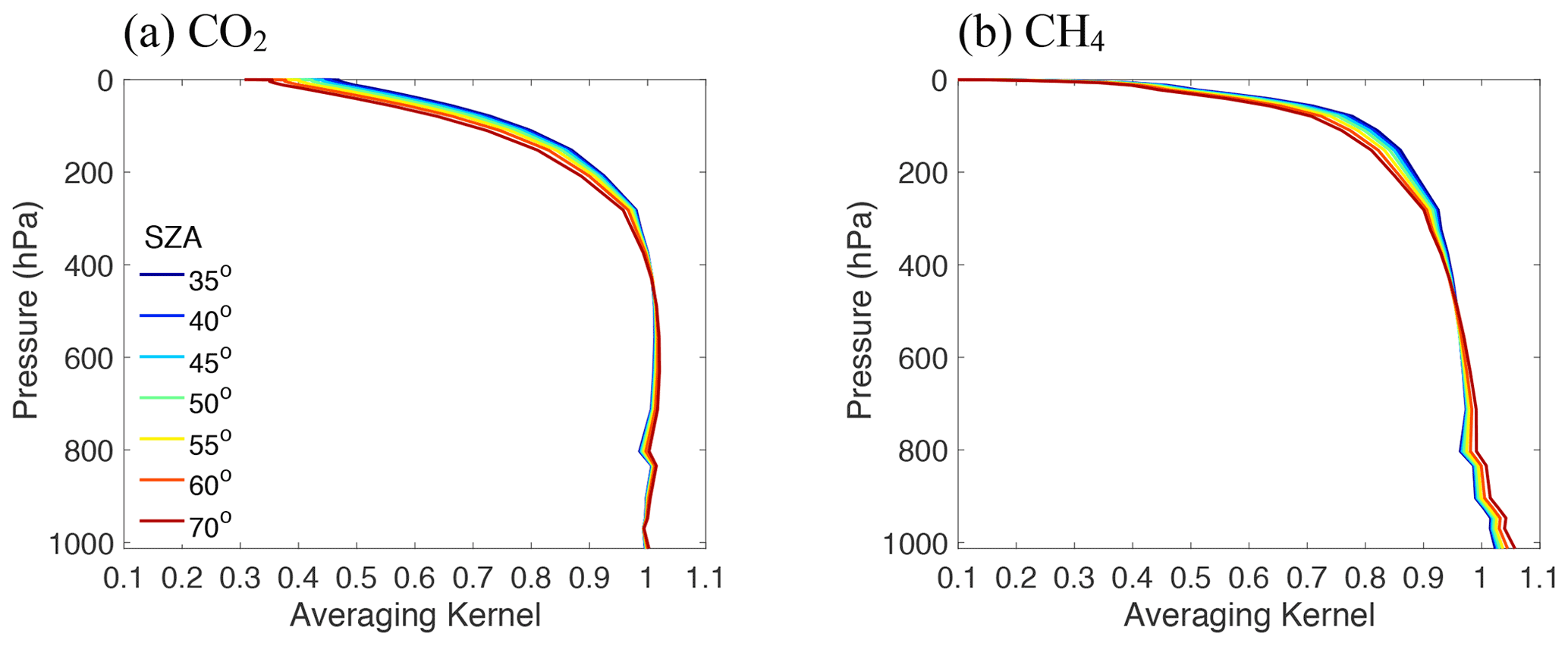
Figure 9Examples of column averaging kernels for (a) CO2 and (b) CH4 with different SZAs. These are from observations of the Santa Anita surface target on 28 September 2013.
3.4 Post-processing
After obtaining the SCDs for O2, CO2, and CH4, XCO2 and XCH4 can be calculated as follows:
where the constant 0.2095 is the column-averaged dry-air mixing ratio of O2 in the atmosphere. In the post-processing, multiple filters are applied to ensure good retrieval quality. First, retrievals that fail to converge after 15 iterations according to the procedure outlined in Eq. (6) are excluded. Second, the spectral fitting residual (RMSE) for each window should be smaller than 0.01 for all four bands. Third, outliers in retrieved state vector parameters, including O2, CO2, and CH4 SCDs, which have a large impact on XCO2 and XCH4, are filtered. In this study, we define outliers as values that are more than 3 standard deviations away from the mean. For retrievals of CLARS-FTS observations from June 2013 to May 2014, about 80 % of all pre-filtered observations pass the post-processing filters.
The goal of applying the GFIT3 algorithm to simulated synthetic spectra is to assess the performance of the algorithm in retrieving XCO2 and XCH4 and to quantify the impacts on the accuracy due to factors such as aerosol scattering, imperfect meteorological data, RTM errors, uncertainty in gas absorption, and instrument noise. In this study, we primarily concentrate on three potentially important error sources: imperfect characterization of aerosol scattering, assumptions about the vertical distributions of CO2 and CH4, and biases due to usage of the O-PCA RTM.
We first generate synthetic spectra using LIDORT with high accuracy (32 streams) to reproduce the “true” spectra under three aerosol loading scenarios (total column AOD=0.01, 0.05, and 0.1), which covers the AOD range for non-cloudy days based on Caltech AERONET measurements (Appendix Fig. A2). Given that CLARS-FTS observes large air mass factors (more than 8 times the vertical column) in the PBL because of the long slant column in the line of sight, the aerosol loading along the slant path is much higher than the column AOD. To simulate the synthetic spectra, we use 3-hourly aerosol composition data from MERRA aerosol reanalysis and other optical properties (SSA and phase function) from the GOCART model (Sect. 3.2.2). CO2 and CH4 vertical profiles are derived as described in Sect. 3.2.2. The hourly variability in CH4 in the PBL is assumed to be the same as that in CO2 since they are co-emitted and follow a similar atmospheric mixing process. Surface albedos for the O2, WCO2, CH4, and SCO2 bands are estimated from CLARS-FTS observations. All other inputs are the same as the state vector described in Sect. 3.2.2. Measurement noise (which we assume to be white noise with a mean of 0 and a standard deviation of 1SNR) is added to generate the synthetic spectra as a proxy for CLARS-FTS observations. We test the GFIT3 algorithm on the synthetic spectra for the three surface targets at Santa Anita, Santa Fe, and West Pasadena over a wide range of observing geometries encompassing four seasons (January, April, July, and October) and 5 h from early morning to late afternoon (∼ 08:00–09:00, 10:00–11:00, 12:00–13:00, 14:00–15:00, 16:00–17:00). Since data in the early morning and late afternoon hours may not be available in winter, we select observations from the available daytime data with a time step of at least 1 h. In total, 60 different observation scenarios are selected.
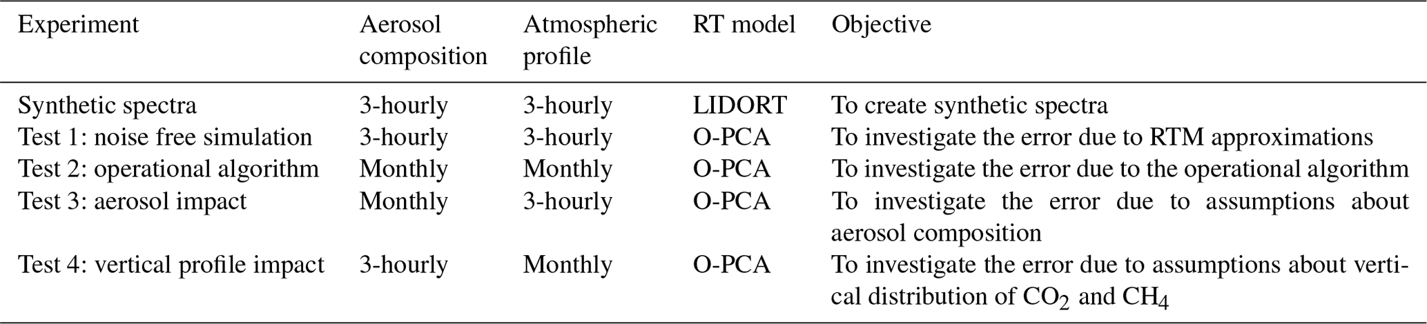
We conduct four retrieval tests on the synthetic spectra, as listed in Table 2. In Test 1, we assume perfect knowledge of aerosol composition and GHG profiles. The goal is to assess the capability of O-PCA and the inverse framework for retrieving XCO2 and XCH4. In Test 2, we use O-PCA but with monthly average aerosol composition and GHG profiles. The goal is to investigate retrieval uncertainty due to assumptions about aerosols and GHG profiles, as well as RT calculation approximations. Test 3 is similar to Test 2, except that we use 3-hourly GHG profiles. The goal is to isolate the impact of uncertainty in aerosol composition. Test 4 is also similar to Test 2, except that we use 3-hourly aerosol composition. The goal is to isolate the impact of imperfect knowledge of GHG vertical distribution. For each observation scenario in these tests, we calculate the difference between the retrieved state vector and the “truth” that was used to generate the synthetic spectra. The retrieval error (in percentage) is defined as the ratio of the calculated difference to the “truth”.
Figure 10 shows results from Test 1. It is evident that all simulations have a mean absolute error (MAE) of less than 0.5 %. The retrieval error, however, increases as AOD increases. In the haziest scenario (AOD=0.1), the largest retrieval error is around 1 %. Results from Test 2 (Fig. 11) are broadly similar to those from Test 1. The errors are generally larger than those in Test 1 due to the bias in aerosol optical properties and atmospheric profiles. On average, the MAEs are less than 1 %; the largest errors are greater than 2 %. The bias in the retrieved AOD is smaller at larger AOD values because of the stronger aerosol scattering signal. Moreover, the bias in ALH is about −10 % on average, indicating an average error of less than 1 km. Figure 12 shows results from tests 3 and 4. No clear correlation can be observed between bias in XCO2 and XCH4 retrievals and that in aerosol optical properties for either coarse- or fine-mode aerosols. This indicates that a combination of fine- and coarse-mode aerosols is able to accurately capture the scattering effects. On the other hand, there is a clear correlation between bias in the trace gas columns and that in PBL enhancement (defined as the difference in PBL GHG mixing ratios between 3-hourly and monthly a priori atmospheric profiles). However, the MAE is still almost always less than 1 %.
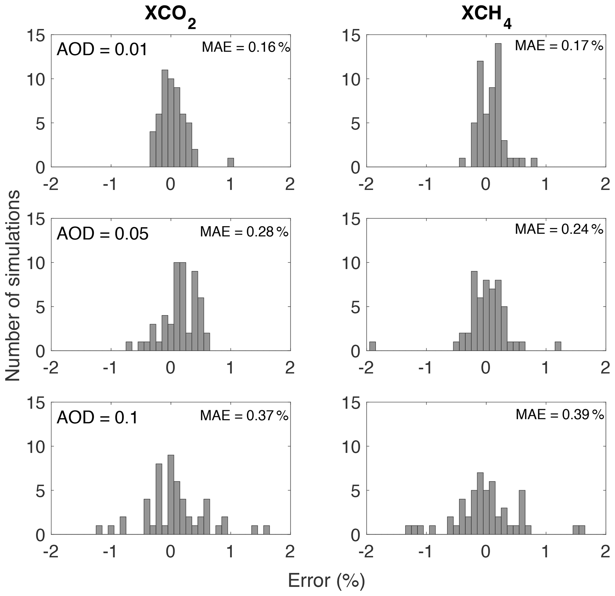
Figure 10Results for Test 1. Errors in retrieved XCO2 and XCH4 are quantified for simulations with three different values of AOD (0.01, 0.05, and 0.1). The errors arise mainly due to the bias caused by the O-PCA approximation compared to the exact atmospheric radiative transfer process. MAE represents the mean absolute error.
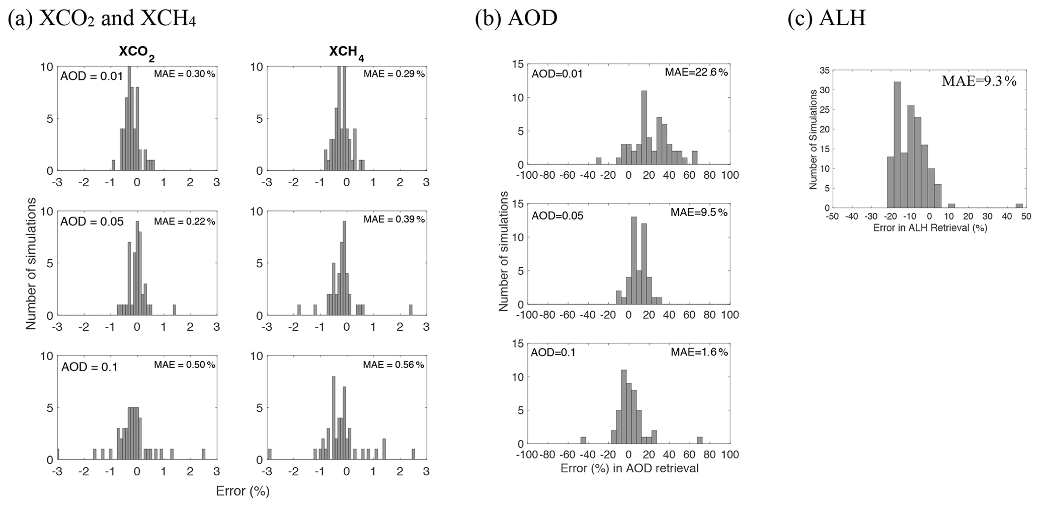
Figure 11Results for Test 2. Errors in retrieved (a) XCO2 and XCH4 for three different values of AOD (0.01, 0.05, and 0.1), (b) AOD for the same scenarios as in (a), and (c) ALH for all AOD scenarios. The errors have contributions from biases due to the O-PCA RTM and due to the imperfect knowledge of aerosol optical properties and vertical distribution of atmospheric trace gases.
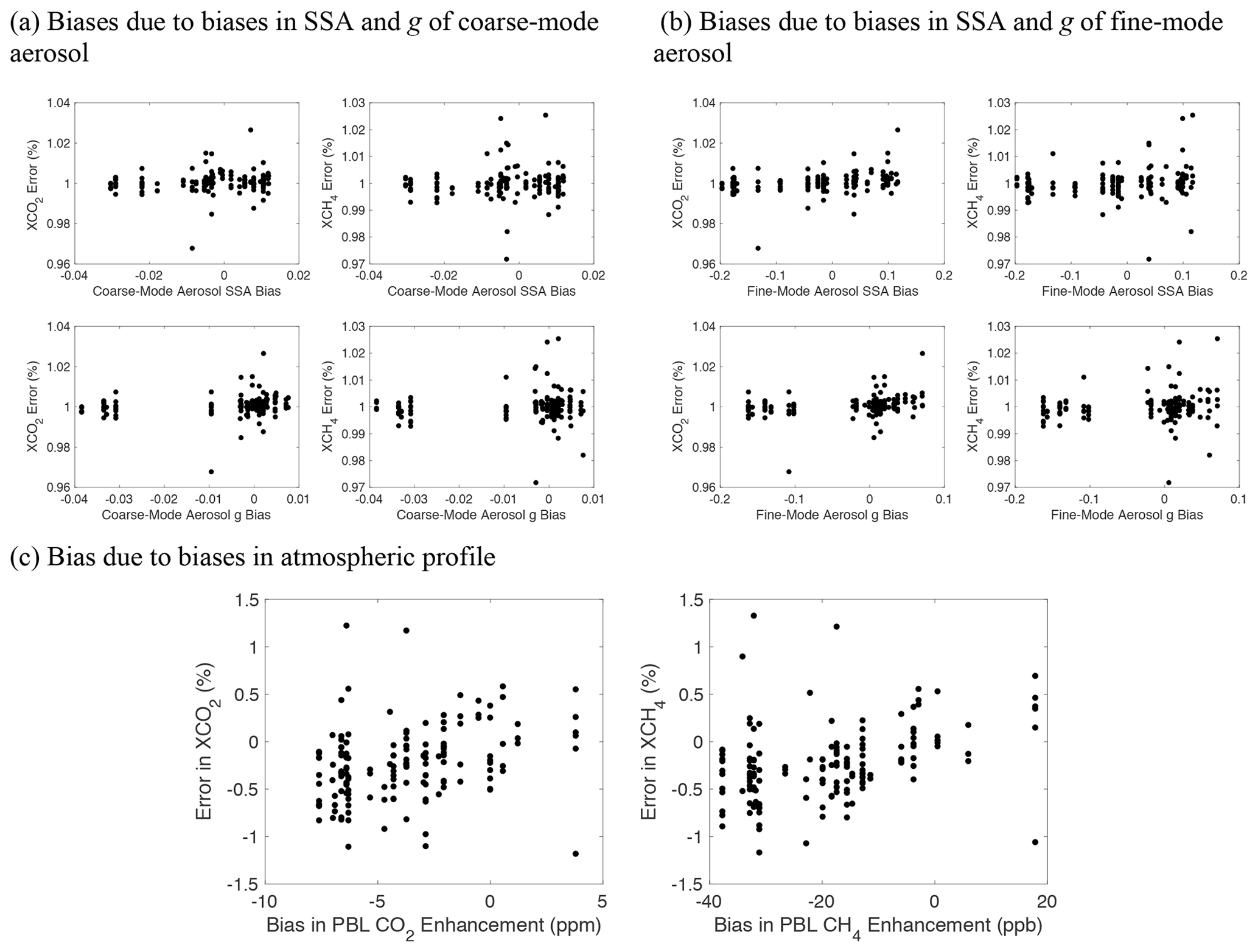
Figure 12Results for Test 3 (a and b) and Test 4 (c). Panels (a) and (b) show XCO2 and XCH4 biases as a function of biases in SSA and g (asymmetry factor) of coarse- and fine-mode aerosol, respectively. Panel (c) shows the same as a function of biases in PBL CO2 and CH4 enhancement. This bias is defined as the difference in PBL GHG mixing ratios between 3-hourly and monthly a priori atmospheric profiles.
Table 2Synthetic experiments to assess the impact of RTM, aerosol composition, and GHG profiles on retrievals of XCO2 and XCH4 from CLARS-FTS observations.
We applied the GFIT3 retrieval algorithm to 1 year of CLARS observations from June 2013 to May 2014. Over this period, CLARS-FTS spent a large portion of measurement time observing the Santa Anita, Santa Fe, and West Pasadena targets. Therefore, these three surface reflection points are our focus in this section. In total there are 36 170 observed spectra from CLARS-GFIT. After pre-processing, we obtain 12 911 spectra that pass the filters for processing by the GFIT3 algorithm. Most of the retrievals converge after less than 10 iterations. However, about 20 % of the measurements fail to converge, and another 20 % fail to pass the post-processing filters; these are discarded. Eventually, 7733 spectra are available for further analysis.
5.1 Residuals from spectral fitting
Figure 13 shows normalized residuals with respect to the continuum level from spectral fitting for the O2, WCO2, CH4, and SCO2 bands. The RMSE values are less than 1 %, and the majority of residuals are less than 0.5 %. The SCO2 band shows a larger residual compared to the other bands, partly due to imperfect spectroscopic data (Crisp et al., 2012) and partly due to the large aerosol scattering contribution, especially in the strong absorption lines (of which there are several due to the high spectral resolution of CLARS-FTS). It is instructive to compare these results with fitting residuals from CLARS-GFIT (Appendix Fig. A3), in which aerosol scattering is neglected. It is evident that the residuals from GFIT3, especially in the SCO2 band, are significantly smaller. In the GFIT3 algorithm, the aerosols are primarily constrained by the O2 and the SCO2 bands. This is because a priori atmospheric pressure is very accurate (∼0.2 % uncertainty) and O2 concentration well known, thereby resulting in the O2 absorption spectra providing strong constraints on the aerosol scattering effects. For the SCO2 band, since most of the absorption lines are saturated, any extra radiance in this spectral region is attributable to aerosol scattering. Ignoring aerosol scattering results in higher residuals, especially for the strong absorption lines (Appendix Fig. A3). Fitting residuals are significantly reduced using GFIT3. Results from this study suggest that the effects of scattering in the observed spectra can be accurately characterized by the aerosol models used in the GFIT3 algorithm. Not accounting for scattering leads to large spectral fitting residuals, and therefore large biases, in GHG retrievals.
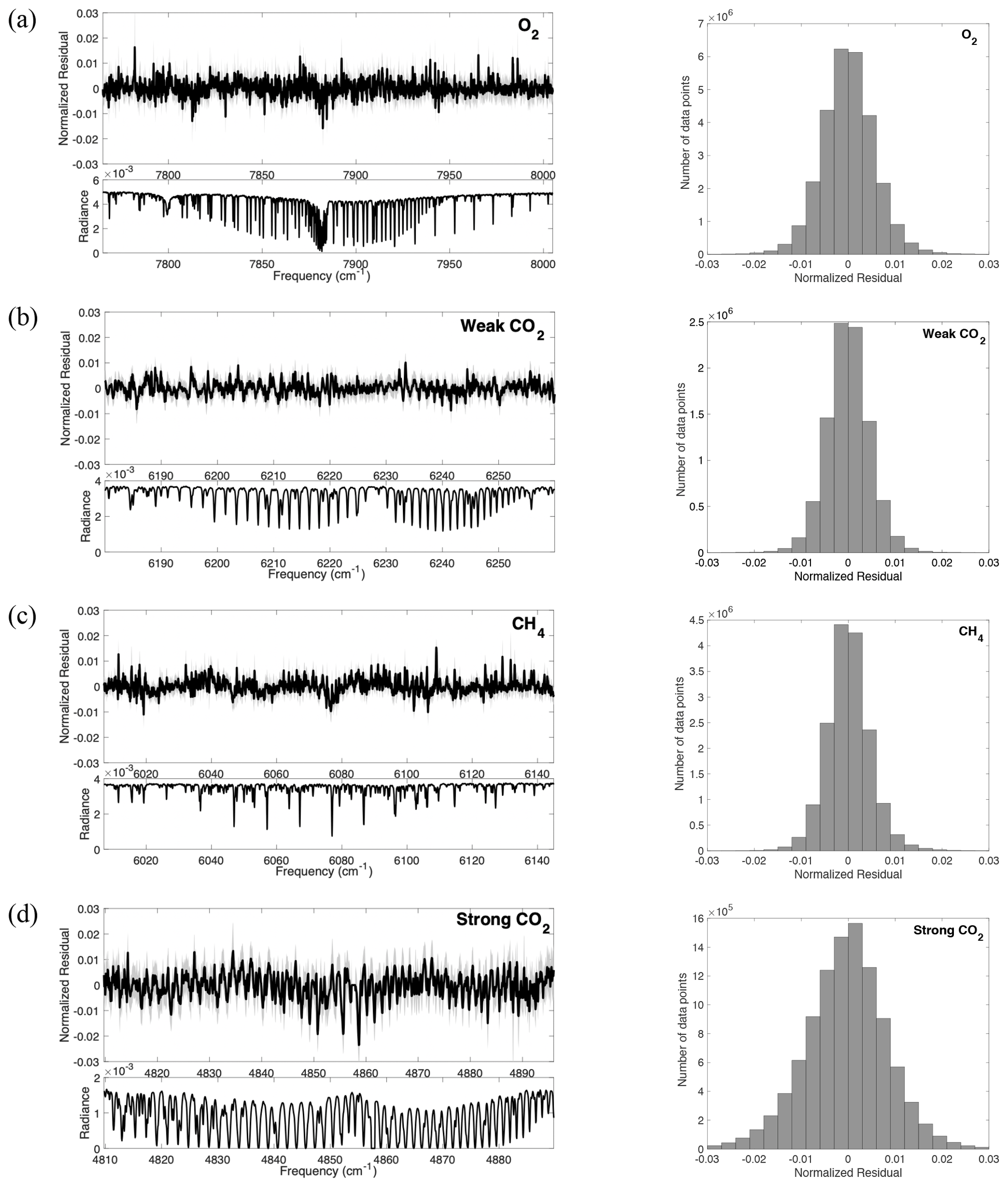
Figure 13(a) Upper left: median fitting residual (black) and ±1σ range (grey) for the O2 band. Lower left: sample measured spectrum. Right: histogram of fitting residuals. Panels (b–d) are the same as (a) but for the weak CO2 band, the CH4 band, and the strong CO2 band, respectively.
5.2 Comparison of retrieved AOD with AERONET and ALH with MiniMPL
We compare the retrieved AOD with ground-based AERONET observations at Caltech. AERONET is a global ground-based aerosol monitoring network (Holben et al., 1998) that has been providing high-accuracy measurements of total AOD from the ultraviolet to the near infrared. The AERONET instrument at Caltech is located on the university campus in Pasadena, which is geographically close to the Santa Anita, Santa Fe, and West Pasadena surface targets. The Caltech AERONET measurements cover the wavelength range from 340 to 1020 nm. To derive the AOD in the O2 1Δ band, we extrapolate from AERONET measurements using the Ångström exponent law (Seinfeld and Pandis, 2006). Figure 14 shows that the retrieved AOD is in good agreement with Caltech AERONET AOD, with RMSE values of about 0.02. The AERONET AOD uncertainty is on the order of 0.01–0.02 in the 0.34–0.87 µm spectral range (Eck et al., 1999); our estimated RMSE value of 0.02 is therefore very close to the noise level. The difference is larger for higher AOD values. This effect may be due to two reasons. First, GFIT3 retrievals have higher uncertainty at large AOD values because of the magnification of biases due to the misrepresentation of aerosol optical properties. Second, CLARS-FTS and AERONET observe different parts of the atmosphere due to differences in their observing geometries. Considering the spatial heterogeneity of aerosol distribution, such a difference between retrieved and observed AOD is expected. The retrieved ALH values agree closely with MiniMPL observations (Fig. 15); however, they do not have significant correlation on a point-by-point basis (not shown). This suggests the difficulty in constraining ALH when it is jointly retrieved with GHGs. The signal from ALH may be interfered with by the imperfect characterization of other factors that existing full physics algorithms cannot resolve. However, when ALH is retrieved independently using specifically targeted O2 absorption lines, high accuracy can be achieved (Zeng et al., 2019). This suggests the potential of a two-step procedure, as proposed in Zeng et al. (2020a), in which the O2 absorption lines are used to provide strong constraints on AOD and ALH. The improved AOD and ALH estimates can then be used as inputs for the retrieval of GHGs.

Figure 14AOD comparison between measurements from the Caltech AERONET site and GFIT3 retrievals. The AERONET AOD at 1.27 µm is extrapolated from actual AERONET observations using the Ångström exponent law. Histograms of the difference between AERONET and GFIT3 retrievals are also included.

Figure 15Comparison of effective ALH from the MiniMPL lidar instrument on the Caltech campus and GFIT3 retrievals for the Santa Anita, Santa Fe, and West Pasadena surface targets.
5.3 Retrievals of XCO2 and XCH4
Figure 16 compares XCO2 and XCH4 retrievals from GFIT3 (after post-processing) and CLARS-GFIT. In general, when aerosols are not accounted for in the retrieval, as in CLARS-GFIT, XCO2 and XCH4 are overestimated (see discussion in Sect. 6.2). The bias can be up to about 10 % for both XCO2 and XCH4. The scatter plots indicate that the differences in XCO2 and XCH4 are significantly correlated with AOD. The correlation coefficients are higher for Santa Anita probably because of the smaller changes in scattering angle (and therefore aerosol effects) compared to the other two surface targets. The XCO2 and XCH4 differences are in the range of 10–30 ppm (parts per million) and 50–150 ppb, respectively, for an AOD value of 0.05 in the 1Δ absorption band. Since CO2 and CH4 are retrieved at similar wavelengths, the biases in XCO2 and XCH4 retrievals due to aerosol scattering are expected to be comparable. The impact on the retrieved ratio in the presence of aerosols is further discussed in Sect. 6.1. Appendix Fig. A4 shows comparisons for all 28 surface targets based on available measurements from June 2013 to May 2014. In comparison to the three sites close to the CLARS location (Santa Anita, Santa Fe, and West Pasadena), for sites that are further away, valid retrievals that pass the filters have lower AOD values. This is because of their longer slant paths in the PBL, leading to a larger scattering effect even under the same vertical aerosol loading.
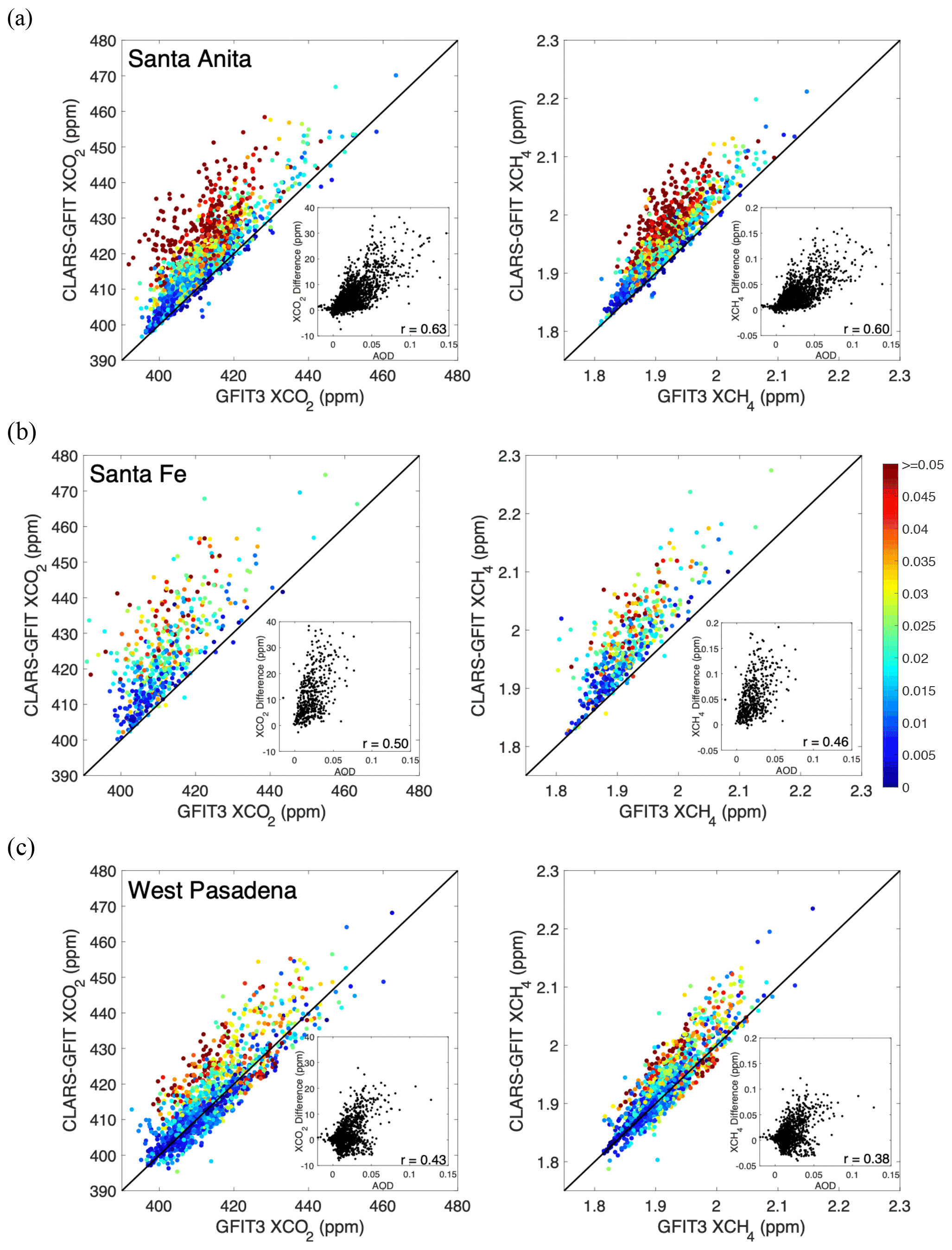
Figure 16Comparison of (left) XCO2 and (right) XCH4 retrievals from GFIT3 and CLARS-GFIT for the (a) Santa Anita, (b) Santa Fe, and (c) West Pasadena surface reflection targets. The data points are color-coded by the retrieved AOD. The insets show scatter plots between retrieved AOD and the difference in XCO2 or XCH4 between GFIT3 and CLARS-GFIT.
6.1 Testing the assumption that the ratio between XCH4 and XCO2 is not affected by aerosol scattering
The tracer–tracer ratio method to retrieve CH4 emissions based on CO2 emissions or CH4 concentration based on CO2 concentration assumes that the ratio cancels out any systematic errors caused by aerosol scattering in the two bands (e.g., Frankenberg et al., 2005; Parker et al., 2011; Wong et al., 2015, 2016; He et al., 2019). However, the fact that the spectral regions do not exactly overlap and that the line intensities have different strengths may reduce the validity of this assumption. Since XCO2 and XCH4 are simultaneously retrieved from both GFIT3 and CLARS-GFIT, these retrievals serve as good datasets for testing the ratioing assumption. Figure 17 shows a scatter plot between CLARS-GFIT ratios and those from GFIT3. No systematic bias is observed from this comparison, suggesting the high accuracy of using the tracer–tracer ratio method to accurately estimate CH4 emissions using remote sensing measurements in the presence of aerosols.

Figure 17Scatter plot of the ratio from GFIT3 and CLARS-GFIT. The 1:1 line is shown in black. The red line denotes the best fit using type II linear regression to fit the data. The equation for the regression fit is also shown.
6.2 Impact of aerosol scattering on XCO2 and XCH4 retrievals regulated by surface reflectance
The effects of aerosol scattering and surface reflectance on modifying the path of solar radiation, and thereby introducing biases in trace gas retrievals, are coupled. A darker surface means a relatively higher contribution from aerosol scattering that will shorten the expected light path. On the other hand, in the presence of a brighter surface, enhanced multiple scattering between the surface and the aerosols may lead to a longer light path. With an RTM, this coupling effect can be explicitly characterized. In general, in the presence of aerosols, XCO2 (or XCH4) will be overestimated if scattering is not accounted for, according to Eqs. (10) and (11). This is because there is larger bias (underestimation) in O2 SCD than in CO2 (or CH4) SCD due to higher AOD at the O2 wavelength. According to MERRA reanalysis data, the AOD ratio between 1.6 and 1.27 µm is about 0.8. However, this is assuming that the surface reflectance is relatively unchanged between the two bands. In fact, the surface is usually darker in the 1.6 µm CO2 band than in the 1.27 µm O2 band. According to our estimates, the reflectance ratio between the two bands is about 0.5–0.8, depending on the composition of the target (soil, vegetation, buildings, etc.). As a result, the darker surface at 1.6 µm may compensate for the lower AOD and increase the relative aerosol scattering contribution.
If the reflectance ratio is close to 1 (no spectral dependence), the XCO2 (or XCH4) bias will be primarily determined by the AOD ratio. Here we assume the aerosols are mostly non-absorbing or do not have a strong spectral dependence of absorption. However, if the reflectance ratio is small (strong spectral dependence), the surface is much darker in the CO2 band than in the O2 band. In this case, it is possible for the surface darkening effect to be more dominant than the AOD effect in driving the bias (underestimation) of retrieved XCO2 (or XCH4). For example, the West Pasadena location is special in that it is close to a park, which has different land use types compared to the other surface targets. This target has a much lower reflectance ratio than other locations (Appendix Fig. A5), which may explain the underestimation by CLARS-GFIT compared to GFIT3 for this location, as seen in Figs. 14c and A4.
6.3 Post-retrieval analysis of fitting residual and goodness of fit
The benefit of using the GFIT spectroscopy database is that it has been carefully evaluated based on highly accurate TCCON observations. To further investigate the errors in spectroscopy, an important contributor to the forward model error in Eq. (1), we apply principal component analysis (PCA) to the fitting residuals. This analysis method has been used by the OCO-2/3 operational algorithm to correct for errors in CO2 spectroscopic parameters and the atmospheric state (O'Dell et al., 2018). The three principal components (PCs) with the largest variance are shown in Appendix Fig. A6. The features in these PCs are mostly related to spectroscopic uncertainties. These PCs might be related to line width, instrument effects, and the solar spectrum. For example, PC-3 from the WCO2 band appears to be correlated with absorption features that may be attributed to very small changes in the line width. However, this PC can only explain a few percent of the residual variance. Overall, there are no PCs that can explain more than 10 % of the variance in the fitting residual. This is because the fitting residual itself is very close to random and without large systematic errors. We therefore believe that spectroscopic errors should not be a major issue here.
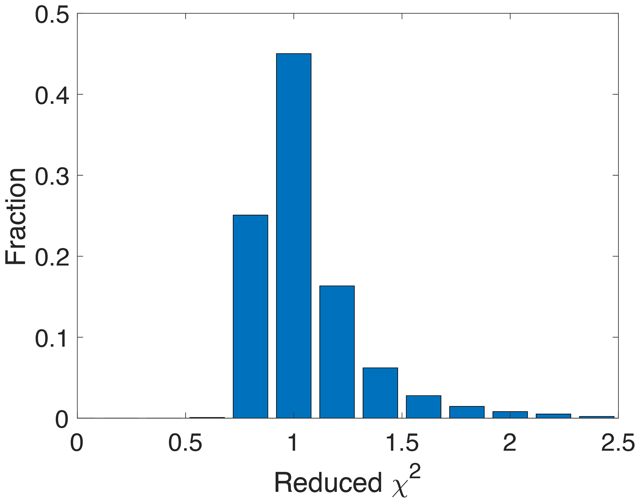
The reduced χ2, which is the χ2 from Eq. (2) divided by the total number of measurements and state vector elements, infers the goodness of fit and can be used to evaluate the error covariance matrix. Theoretically, if the error covariance matrix is properly implemented in the retrieval algorithm, the reduced χ2 should be close to 1 after convergence, which means that the fitting residuals are consistent with the detector noise estimates. The histogram of reduced χ2 from all converged retrievals (Appendix Fig. A7) indicates that most of the retrievals have a χ2 close to 1 (83 % having χ2 less than 1.5). This indicates that the error covariance matrix used in the retrieval algorithm, which assumes that measurement noise is uncorrelated between different spectral channels, is realistic. It should be noted that inaccuracies in the spectroscopic input data and improperly modeled instrument effects may contribute to the small deviation of χ2 from unity.
In this study, we developed GFIT3, a full physics algorithm to retrieve trace gases in the presence of aerosols, and demonstrated its performance by retrieving XCO2 and XCH4 from CLARS-FTS measurements. This algorithm simultaneously retrieves fine- and coarse-mode aerosol properties including AOD and ALH. Inverse experiments based on synthetic spectra indicate that the uncertainty in CLARS-FTS retrievals of XCO2 and XCH4 due to uncertainty in the RTM, aerosol scattering, and atmospheric profile, which constitute the three most important sources of error, is less than 1 % (or less than ∼4 ppm for XCO2 and ∼20 ppb for XCH4). The retrieval uncertainty for real CLARS-FTS observations is partly due to the imperfect characterization of aerosol properties. Nonetheless, we find that the retrieved AOD has good agreement with AERONET measurements. Unfortunately, direct comparison of XCO2 and XCH4 with existing TCCON data at Caltech is not feasible. On one hand, CLARS-FTS cannot directly target the TCCON site at Caltech due to mountain ridges that block the line of sight. On the other, TCCON uses directly transmitted solar spectra to measure GHG columns, which have different geometries from CLARS observations; the spatial heterogeneity of GHG distributions between the incident and reflected solar paths in the boundary layer make the results difficult to compare.
Future research will focus on developing a “divide and conquer” algorithm for retrieving aerosol properties and GHGs in order to further improve the accuracy of GHG retrievals. The basic idea is to use a two-step procedure. First, O2 absorption lines will be used to constrain the AOD and ALH based on a spectral sorting technique (Zeng et al., 2019). These values will then provide constraints for AOD and ALH (with uncertainty estimates) for the retrieval of GHGs.

Figure A1(a) Time series of O2 volume mixing ratio (VMR) scale factor (VSF) and (b) histogram of VSF. The VSF value (indicated by the dashed red line) of ∼1.02 represents situations when the atmosphere is clear. See Sect. 3.1.1 for details.

Figure A2AOD in the 1.27 µm O2 absorption band estimated from AERONET observations (2010–2017).
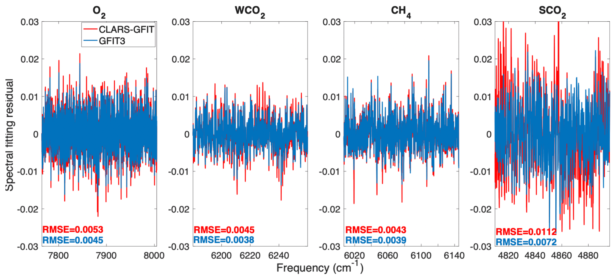
Figure A3Example of spectral fitting residuals from the CLARS-GFIT (red; ignoring aerosol scattering) and GFIT3 (blue; accounting for aerosol scattering) algorithms for the O2, WCO2, CH4, and SCO2 spectral windows. The spectral fitting RMSEs are also indicated. This example is for an observation over the West Pasadena surface target on 28 September 2013 with a solar zenith angle of 65∘.

Figure A4Comparison of XCO2 retrievals from GFIT3 and CLARS-GFIT for all surface reflection targets. The data points are color-coded by the retrieved AOD.
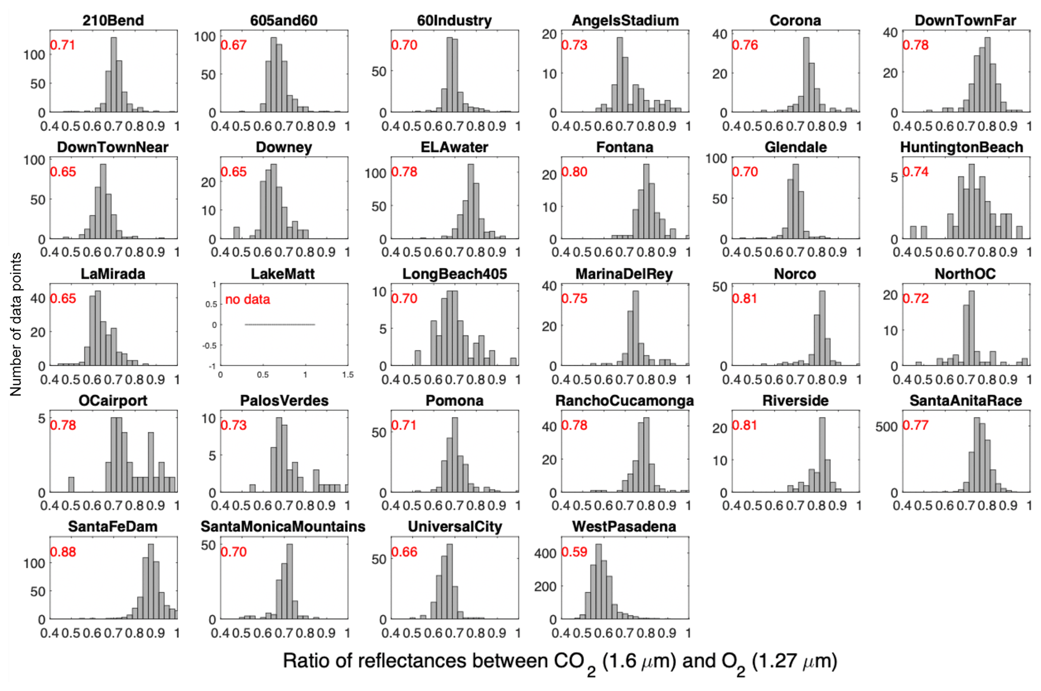
Figure A5Histogram of the ratio of reflectance between the WCO2 and O2 bands for all the surface targets. The reflectance values are obtained from GFIT3 retrievals. The number in red is the average ratio for the surface target.

Figure A6Mean radiance spectrum and the three leading PCs ranked by the variance explained by these PCs, obtained by applying PCA on the fitting residuals, for the (a) O2, (b) WCO2, (c) CH4, and (d) SCO2 bands. The variance explained by each PC is also indicated.
CLARS-FTS data are available from https://data.caltech.edu/records/1948 (last access: 21 September 2021) or https://doi.org/10.22002/D1.1948 (Zeng, 2021), and part of the CLARS data is also available from the NASA Megacities Project at https://megacities.jpl.nasa.gov (Sander and Pongetti, 2020). The MiniMPL data are available from the NASA Megacity Project data portal: https://megacities.jpl.nasa.gov/portal/ (Ware et al., 2020). AERONET data for the Caltech site are available from https://aeronet.gsfc.nasa.gov/new_web/photo_db_v3/CalTech.html (Stutz, 2021).
ZZ designed this study, conducted the experiments, analyzed the results, and wrote the paper. VN developed the O-PCA code and provided guidance on RT modeling. FX provided guidance on optimal estimation. SC assisted with the RT calculations. FG analyzed the aerosol observations and made comparisons. TJP collected the CLARS data, and KS contributed to spectroscopy analysis. GT provided guidance on using GFIT. YLY and SPS supervised this study. All authors proofread and commented on the paper.
The authors declare that they have no conflict of interest.
Publisher's note: Copernicus Publications remains neutral with regard to jurisdictional claims in published maps and institutional affiliations.
A portion of this research was carried out at the Jet Propulsion Laboratory, California Institute of Technology, under a contract with the National Aeronautics and Space Administration (80NM0018D0004). We thank Jochen Stutz from UCLA and his staff for their effort in establishing and maintaining the Caltech AERONET site.
Zhao-Cheng Zeng is supported by subcontract funds from the Jet Propulsion Lab (Sponsor Award Number: 1658775). A part of this research has been supported by the National Aeronautics and Space Administration (grant no. 80NM0018D0004).
This paper was edited by Helen Worden and reviewed by Brian Connor and one anonymous referee.
Bertaux, J.-L., Hauchecorne, A., Lefèvre, F., Bréon, F.-M., Blanot, L., Jouglet, D., Lafrique, P., and Akaev, P.: The use of the 1.27 µm O2 absorption band for greenhouse gas monitoring from space and application to MicroCarb, Atmos. Meas. Tech., 13, 3329–3374, https://doi.org/10.5194/amt-13-3329-2020, 2020.
Bril, A., Oshchepkov, S., and Yokota, T.: Application of a probability density function-based atmospheric light-scattering correction to carbon dioxide retrievals from GOSAT over-sea observations, Remote Sens. Environ., 117, 301–306. 2012.
Butz, A., Hasekamp, O. P., Frankenberg, C., and Aben, I.: Retrievals of atmospheric CO2 from simulated space-borne measurements of backscattered near-infrared sunlight: accounting for aerosol effects, Appl. Optics, 48, 3322–3336, https://doi.org/10.1364/AO.48.003322, 2009.
Butz, A., Guerlet, S., Hasekamp, O., Schepers, D., Galli, A., Aben, I., Frankenberg, C., Hartmann, J.-M., Tran, H., Kuze, A., Keppel-Aleks, G., Toon, G., Wunch, D., Wennberg, P., Deutscher, N., Griffith, D., Macatangay, R., Messerschmidt, J., Notholt, J., and Warneke, T.: Toward accurate CO2 and CH4 observations from GOSAT, Geophys. Res. Lett., 38, L14812, https://doi.org/10.1029/2011GL047888, 2011.
Chin, M., Ginoux, P., Kinne, S., Torres, O., Holben, B. N., Duncan, B. N., Martin, R. V., Logan, J. A., Higurashi, A., and Nakajima, T.: Tropospheric Aerosol Optical Thickness from the GOCART Model and Comparisons with Satellite and Sun Photometer Measurements, J. Atmos. Sci., 59, 461–483, https://doi.org/10.1175/1520-0469(2002)059<0461:TAOTFT>2.0.CO;2, 2002.
Connor, B. J., Sherlock, V., Toon, G., Wunch, D., and Wennberg, P. O.: GFIT2: an experimental algorithm for vertical profile retrieval from near-IR spectra, Atmos. Meas. Tech., 9, 3513–3525, https://doi.org/10.5194/amt-9-3513-2016, 2016.
Crisp, D., Fisher, B. M., O'Dell, C., Frankenberg, C., Basilio, R., Bösch, H., Brown, L. R., Castano, R., Connor, B., Deutscher, N. M., Eldering, A., Griffith, D., Gunson, M., Kuze, A., Mandrake, L., McDuffie, J., Messerschmidt, J., Miller, C. E., Morino, I., Natraj, V., Notholt, J., O'Brien, D. M., Oyafuso, F., Polonsky, I., Robinson, J., Salawitch, R., Sherlock, V., Smyth, M., Suto, H., Taylor, T. E., Thompson, D. R., Wennberg, P. O., Wunch, D., and Yung, Y. L.: The ACOS CO2 retrieval algorithm – Part II: Global X data characterization, Atmos. Meas. Tech., 5, 687–707, https://doi.org/10.5194/amt-5-687-2012, 2012.
Eck, T. F., Holben, B. N., Reid, J. S., Dubovik, O., Smirnov, A., O'Neill, N. T., Slutsker, I., and Kinne, S.: Wavelength dependence of the optical depth of biomass burning, urban, and desert dust aerosols, J. Geophys. Res.-Atmos., 104, 31333–31349, 1999.
Fletcher, R.: A modified Marquardt subroutine for nonlinear least squares fitting, Report, Atomic Energy Research Establishment, Harwell, England, 1971.
Frankenberg, C., Meirink, J. F., van Weele, M., Platt, U., and Wagner, T.: Assessing methane emissions from global space-borne observations, Science, 308, 1010–1014, https://doi.org/10.1126/science.1106644, 2005.
Fu, D., Pongetti, T. J., Blavier, J.-F. L., Crawford, T. J., Manatt, K. S., Toon, G. C., Wong, K. W., and Sander, S. P.: Near-infrared remote sensing of Los Angeles trace gas distributions from a mountaintop site, Atmos. Meas. Tech., 7, 713–729, https://doi.org/10.5194/amt-7-713-2014, 2014.
He, L., Zeng, Z.-C., Pongetti, T. J., Wong, C., Liang, J., Gurney, K., Newman, S., Yadav, V., Verhulst, K., Miller, C., Duren, R., Frankenberg, C., Wennberg, P. O., Shia, R.-L., Yung, Y. L., and Sander, S. P.: Atmospheric methane emissions correlate with natural gas consumption from residential and commercial sectors in Los Angeles, Geophys. Res. Lett., 46, 8563–8571, https://doi.org/10.1029/2019GL083400, 2019.
Hersbach, H., Bell, B., Berrisford, P., Hirahara, S., Horányi, A., Muñoz-Sabater, J., Nicolas, J., Peubey, C., Radu, R., Schepers, D., Simmons, A., Soci, C., Abdalla, S., Abellan, X., Balsamo, G., Bechtold, P., Biavati, G., Bidlot, J., Bonavita, M., Chiara, G. D., Dahlgren, P., Dee, D., Diamantakis, M., Dragani, R., Flemming, J., Forbes, R., Fuentes, M., Geer, A., Haimberger, L., Healy, S., Hogan, R. J., Hólm, E., Janisková, M., Keeley, S., Laloyaux, P., Lopez, P., Lupu, C., Radnoti, G., Rosnay, P. de, Rozum, I., Vamborg, F., Villaume, S., and Thépaut, J.-N.: The ERA5 Global Reanalysis, Q. J. Roy. Meteor. Soc., 146, 1999–2049, https://doi.org/10.1002/qj.3803, 2020.
Holben, B. N., Eck, T. F., Slutsker, I., Tanre, D., Buis, J. P., Set- zer, A., Vermote, E., Reagan, J. A., Kaufman, Y., Nakajima, T., Lavenu, F., Jankowiak, I., and Smirnov, A.: AERONET – A federated instrument network and data archive for aerosol characterization, Remote Sens. Environ., 66, 1–16, 1998.
Irion, F. W., Gunson, M. R., Toon, G. C., Chang, A. Y., Eldering, A., Mahieu, E., Manney, G. L., Michelsen, H. A., Moyer, E. J., Newchurch, M. J., Osterman, G. B., Rinsland, C. P., Salawitch, R. J., Sen, B., Yung, Y. L., and Zander, R.: Atmospheric Trace Molecule Spectroscopy (ATMOS) Experiment Version 3 data retrievals, Appl. Optics, 41, 6968–6979, 2002.
Kalnay, E., Kanamitsu, M., Kistler, R., Collins, W., Deaven, D., Gandin, L., Iredell, M., Saha, S., White, G., Woollen, J., Zhu, Y., Chelliah, M., Ebisuzaki, W., Higgins, W., Janowiak, J., Mo, K. C., Ropelewski, C., Wang, J., Leetmaa, A., Reynolds, R., Jenne, R., and Joseph, D.: The NCEP/NCAR 40-year reanalysis project, B. Am. Meteorol. Soc., 77, 437–471, 1996.
Kopparla, P., Natraj, V., Spurr, R., Shia, R. L., Crisp, D., and Yung, Y. L.: A fast and accurate PCA based radiative transfer model: Extension to the broadband shortwave region, J. Quant. Spectrosc. Ra., 173, 65–71, 2016.
Kopparla, P., Natraj, V., Limpasuvan, D., Spurr, R., Crisp, D., Shia, R. L., Somkuti, P., and Yung, Y. L.: PCA-based radiative transfer: Improvements to aerosol scheme, vertical layering and spectral binning, J. Quant. Spectrosc. Ra., 198, 104–111, 2017.
Kurucz, R. L.: High resolution irradiance spectrum from 300 to 1000 nm, AFRL Transmission Meeting, Lexington, Mass., 15–16 June 2005, 2005.
Levenberg, K.: A method for the solution of certain non-linear problems in least squares, Q. Appl. Math., 2, 164–168, 1944.
Marquardt, D. W.: An algorithm for least squares estimation of non- linear parameters, J. Soc. Ind. Appl. Math., 11, 431–441, 1963.
Natraj, V., Jiang, X., Shia, R.-L., Huang, X., Margolis, J. S., and Yung Y. L.: Application of principal component analysis to high spectral resolution radiative transfer: A case study of the O2 A-band, J. Quant. Spectrosc. Ra., 95, 539–556, https://doi.org/10.1016/j.jqsrt.2004.12.024, 2005.
Natraj, V., Shia, R. L., and Yung, Y. L.: On the use of principal component analysis to speed up radiative transfer calculations, J. Quant. Spectrosc. Ra., 111, 810–816, https://doi.org/10.1016/j.jqsrt.2009.11.004, 2010.
Nelson, R. R., O'Dell, C. W., Taylor, T. E., Mandrake, L., and Smyth, M.: The potential of clear-sky carbon dioxide satellite retrievals, Atmos. Meas. Tech., 9, 1671–1684, https://doi.org/10.5194/amt-9-1671-2016, 2016.
O'Dell, C. W., Connor, B., Bösch, H., O'Brien, D., Frankenberg, C., Castano, R., Christi, M., Eldering, D., Fisher, B., Gunson, M., McDuffie, J., Miller, C. E., Natraj, V., Oyafuso, F., Polonsky, I., Smyth, M., Taylor, T., Toon, G. C., Wennberg, P. O., and Wunch, D.: The ACOS CO2 retrieval algorithm – Part 1: Description and validation against synthetic observations, Atmos. Meas. Tech., 5, 99–121, https://doi.org/10.5194/amt-5-99-2012, 2012.
O'Dell, C. W., Eldering, A., Wennberg, P. O., Crisp, D., Gunson, M. R., Fisher, B., Frankenberg, C., Kiel, M., Lindqvist, H., Mandrake, L., Merrelli, A., Natraj, V., Nelson, R. R., Osterman, G. B., Payne, V. H., Taylor, T. E., Wunch, D., Drouin, B. J., Oyafuso, F., Chang, A., McDuffie, J., Smyth, M., Baker, D. F., Basu, S., Chevallier, F., Crowell, S. M. R., Feng, L., Palmer, P. I., Dubey, M., García, O. E., Griffith, D. W. T., Hase, F., Iraci, L. T., Kivi, R., Morino, I., Notholt, J., Ohyama, H., Petri, C., Roehl, C. M., Sha, M. K., Strong, K., Sussmann, R., Te, Y., Uchino, O., and Velazco, V. A.: Improved retrievals of carbon dioxide from Orbiting Carbon Observatory-2 with the version 8 ACOS algorithm, Atmos. Meas. Tech., 11, 6539–6576, https://doi.org/10.5194/amt-11-6539-2018, 2018.
Parker, R., Boesch, H., Cogan, A., Fraser, A., Feng, L., Palmer, P. I., Messerschmidt, J., Deutscher, N., Griffith, D. W., Notholt, J., and Wennberg, P. O.: Methane observations from the Greenhouse Gases Observing SATellite: Comparison to ground-based TCCON data and model calculations, Geophys. Res. Lett., 38, L15807, https://doi.org/10.1029/2011GL047871, 2011.
Peters, W., Jacobson, A. R., Sweeney, C., Andrews, A. E., Con- way, T. J., Masarie, K., Miller, J. B., Bruhwiler, L. M. P., Petron, G., Hirsch, A. I., Worthy, D. E. J., van der Werf, G. R., Randerson, J. T., Wennberg, P. O., Krol, M. C., and Tans, P. P.: An atmospheric perspective on North American carbon dioxide ex- change: CarbonTracker, P. Natl. Acad. Sci. USA, 104, 18925–18930, https://doi.org/10.1073/pnas.0708986104, 2007.
Reuter, M., Buchwitz, M., Schneising, O., Noël, S., Rozanov, V., Bovensmann, H., and Burrows, J. P.: A fast atmospheric trace gas retrieval for hyperspectral instruments approximating multiple scattering – Part 1: Radiative transfer and a potential OCO-2 XCO2 retrieval setup, Remote Sens., 9, 1159, https://doi.org/10.3390/rs9111159, 2017.
Rienecker, M. M., Suarez, M. J., Gelaro, R., Todling, R., Bacmeister, J., Liu, R., Bosilovich, M. G., Schubert, S. D., Takacs, L., Kim, G.-K., Bloom, S., Chen, J., Collins, D., Conaty, A., da Silva, A., Gu, W., Joiner, J., Koster, R. D., Lucchesi, R., Molod, A., Owens, T., Pawson, S., Pegion, P., Redder, C. R., Reichle, R., Robertson, F. R., Ruddick, A. G., Sienkiewicz, M., and Woollen, J.: MERRA: NASA's Modern-Era Retrospective Analysis for Research and Applications, J. Climate, 24, 3624–3648, 2011.
Roche, S., Strong, K., Wunch, D., Mendonca, J., Sweeney, C., Baier, B., Biraud, S. C., Laughner, J. L., Toon, G. C., and Connor, B. J.: Retrieval of atmospheric CO2 vertical profiles from ground-based near-infrared spectra, Atmos. Meas. Tech., 14, 3087–3118, https://doi.org/10.5194/amt-14-3087-2021, 2021.
Rodgers, C. D.: Inverse Methods for Atmospheric Sounding: Theory and Practice, World Scientific, Singapore, 2000.
Sander, S. P. and Pongetti, T. J.: CLARS-FTS data, available at: https://megacities.jpl.nasa.gov, last access: 12 December 2020.
Seinfeld, J. and Pandis, S.: Atmospheric chemistry and physics: from air pollution to climate change, Wiley, Inc., New Jersey, USA, p. 1224, 2006.
Sen, B., Toon, G. C., Blavier, J.-F., Fleming, E. L., and Jackman, C. H.: Balloon-borne observations of mid-latitude fluorine abundance, J. Geophys. Res., 101, 9045–9054, 1996.
Somkuti, P., Boesch, H., Natraj, V., and Kopparla, P.: Application of a PCA-based fast radiative transfer model to XCO2 retrievals in the shortwave infrared, J. Geophys. Res.-Atmos., 122, 10477–10496, 2017.
Spurr, R.: LIDORT and VLIDORT: Linearized pseudo-spherical scalar and vector discrete ordinate radiative transfer models for use in remote sensing retrieval problems, in: Light Scattering Reviews 3, 229–275, Springer, Berlin, Heidelberg, 2008.
Spurr, R. and Natraj, V.: A linearized two-stream radia- tive transfer code for fast approximation of multiple- scatter fields, J. Quant. Spectrosc. Ra., 112, 2630–2637, https://doi.org/10.1016/j.jqsrt.2011.06.014, 2011.
Spurr, R., Natraj, V., Lerot, C., Van Roozendael, M., and Loyola, D.: Linearization of the principal component analysis method for radiative transfer acceleration: Application to retrieval algorithms and sensitivity studies, J. Quant. Spectrosc. Ra., 125, 1–17, https://doi.org/10.1016/j.jqsrt.2013.04.002, 2013.
Stutz, J.: AERONET data at the Caltech site, available at: https://aeronet.gsfc.nasa.gov/new_web/photo_db_v3/CalTech.html, last access: 28 September 2021.
Toon, G. C.: Solar line list for GGG2014, TCCON data archive, https://doi.org/10.14291/tccon.ggg2014.solar.R0/1221658, 2014.
Verhulst, K. R., Karion, A., Kim, J., Salameh, P. K., Keeling, R. F., Newman, S., Miller, J., Sloop, C., Pongetti, T., Rao, P., Wong, C., Hopkins, F. M., Yadav, V., Weiss, R. F., Duren, R. M., and Miller, C. E.: Carbon dioxide and methane measurements from the Los Angeles Megacity Carbon Project – Part 1: calibration, urban enhancements, and uncertainty estimates, Atmos. Chem. Phys., 17, 8313–8341, https://doi.org/10.5194/acp-17-8313-2017, 2017.
Wang, S., van der A, R. J., Stammes, P., Wang, W., Zhang, P., Lu, N., Zhang, X., Bi, Y., Wang, P., and Fang, L.: Carbon Dioxide Retrieval from TanSat Observations and Validation with TCCON Measurements, Remote Sens., 12, 2204, https://doi.org/10.3390/rs12142204, 2020.
Ware, J., Kort, E. A. , DeCola, P., and Duren, R.: Mini Micropulse LiDAR (MiniMPL) data at Caltech site, available at: https://megacities.jpl.nasa.gov/portal/, last access: 12 December 2020.
Washenfelder, R. A., Toon, G. C., Blavier, J. F., Yang, Z., Allen, N. T., Wennberg, P. O., Vay, S. A., Matross, D. M., and Daube, B. C.: Carbon dioxide column abundances at the Wisconsin Tall Tower site, J. Geophys. Res.-Atmos., 111, D22305, https://doi.org/10.1029/2006JD007154, 2006.
Wong, C. K., Pongetti, T. J., Oda, T., Rao, P., Gurney, K. R., Newman, S., Duren, R. M., Miller, C. E., Yung, Y. L., and Sander, S. P.: Monthly trends of methane emissions in Los Angeles from 2011 to 2015 inferred by CLARS-FTS observations, Atmos. Chem. Phys., 16, 13121–13130, https://doi.org/10.5194/acp-16-13121-2016, 2016.
Wong, K. W., Fu, D., Pongetti, T. J., Newman, S., Kort, E. A., Duren, R., Hsu, Y.-K., Miller, C. E., Yung, Y. L., and Sander, S. P.: Mapping CH4 : CO2 ratios in Los Angeles with CLARS-FTS from Mount Wilson, California, Atmos. Chem. Phys., 15, 241–252, https://doi.org/10.5194/acp-15-241-2015, 2015.
Wunch, D., Toon, G. C., Blavier, J. F., Washenfelder, R. A., Notholt, J., Connor, B. J., Griffith, D. W. T., Sherlock, V., and Wennberg, P. O.: The Total Carbon Column Observing Network, Philos. T. Roy. Soc. A, 369, 2087–2112, https://doi.org/10.1098/rsta.2010.0240, 2011.
Wunch, D., Toon, G. C., Sherlock, V., Deutscher, N. M., Liu, C., Feist, D. G., and Wennberg, P. O.: Documentation for the 2014 TCCON Data Release, CaltechDATA, https://doi.org/10.14291/TCCON.GGG2014.\hack{\-}DOCUMENTATION.R0/1221662, 2015.
Yang, D., Boesch, H., Liu, Y., Somkuti, P., Cai, Z., Chen, X., Di Noia, A., Lin, C., Lu, N., Lyu, D., and Parker, R. J.: Toward High Precision XCO2 Retrievals from TanSat Observations: Retrieval Improvement and Validation against TCCON Measurements, J. Geophys. Res.-Atmos., 125, p.e2020JD032794, 2020.
Yoshida, Y., Kikuchi, N., Morino, I., Uchino, O., Oshchepkov, S., Bril, A., Saeki, T., Schutgens, N., Toon, G. C., Wunch, D., Roehl, C. M., Wennberg, P. O., Griffith, D. W. T., Deutscher, N. M., Warneke, T., Notholt, J., Robinson, J., Sherlock, V., Connor, B., Rettinger, M., Sussmann, R., Ahonen, P., Heikkinen, P., Kyrö, E., Mendonca, J., Strong, K., Hase, F., Dohe, S., and Yokota, T.: Improvement of the retrieval algorithm for GOSAT SWIR XCO2 and XCH4 and their validation using TCCON data, Atmos. Meas. Tech., 6, 1533–1547, https://doi.org/10.5194/amt-6-1533-2013, 2013.
Zeng, Z.-C.: CLARS-FTS XCH4 and XCO2 retrievals (June 2013–May 2014) from GFIT3 algorithm (Version 1.0), CaltechDATA [data set], https://doi.org/10.22002/D1.1948, 2021.
Zeng, Z.-C. and Sander, S.: CLARS-FTS XCH4 and XCO2 retrievals (June 2013–May 2014) from GFIT3 algorithm (1.0), CaltechDATA [data set], https://doi.org/10.22002/D1.1948, 2021.
Zeng, Z.-C., Zhang, Q., Natraj, V., Margolis, J. S., Shia, R.-L., Newman, S., Fu, D., Pongetti, T. J., Wong, K. W., Sander, S. P., Wennberg, P. O., and Yung, Y. L.: Aerosol scattering effects on water vapor retrievals over the Los Angeles Basin, Atmos. Chem. Phys., 17, 2495–2508, https://doi.org/10.5194/acp-17-2495-2017, 2017.
Zeng, Z.-C., Natraj, V., Xu, F., Pongetti, T. J., Shia, R.-L., Kort, E. A., Toon, G. C., Sander, S. P., and Yung, Y. L.: Constraining Aerosol Vertical Profile in the Boundary Layer Using Hyperspectral Measurements of Oxygen Absorption, Geophys. Res. Lett., 45, 10772–10780 https://doi.org/10.1029/2018GL079286, 2018.
Zeng, Z.-C., Chen, S., Natraj, V., Le, T., Xu, F., Merrelli, A., Crisp, D., Sander, S. P., and Yung, Y. L.: Constraining the vertical distribution of coastal dust aerosol using OCO-2 O2 A-band measurements, Remote Sens. Environ., 236, 111494, https://doi.org/10.1016/j.rse.2019.111494, 2020a.
Zeng, Z.-C., Wang, Y., Pongetti, T., Gong, F.-Y., Newman, S., Li, Y., Natraj, V., Shia, R.-L., Yung, Y. L., and Sander, S. P.: Tracking the Atmospheric Pulse of a North American Megacity from a Mountaintop Remote Sensing Observatory, Remote Sens. Environ., 248, 112000, https://doi.org/10.1016/j.rse.2020.112000, 2020b.
Zeng, Z.-C., Xu, F., Natraj, V., Pongetti, T. J., Shia, R.-L., Zhang, Q., Sander, S. P., and Yung, Y. L.: Remote sensing of angular-dependent scattering of aerosols in a North American megacity, Remote Sens. Environ., 242, 111760, https://doi.org/10.1016/j.rse.2020.111760, 2020c.
- Abstract
- Introduction
- California Laboratory for Atmospheric Remote Sensing (CLARS)
- GFIT3: a full physics approach for retrieving XCO2 and XCH4 from CLARS-FTS observations
- Inversion experiments based on synthetic spectra
- Retrieval results for CLARS-FTS observations
- Discussions
- Conclusions
- Appendix A
- Code and data availability
- Author contributions
- Competing interests
- Disclaimer
- Acknowledgements
- Financial support
- Review statement
- References