the Creative Commons Attribution 4.0 License.
the Creative Commons Attribution 4.0 License.
 | 13 Oct 2021
Atmospheric carbon dioxide measurement from aircraft and comparison with OCO-2 and CarbonTracker model data
Qin Wang
Farhan Mustafa
Lingbing Bu
Shouzheng Zhu
Jiqiao Liu
Weibiao Chen
Accurate monitoring of atmospheric carbon dioxide (CO2) and its distribution is of great significance for studying the carbon cycle and predicting future climate change. Compared to the ground observational sites, the airborne observations cover a wider area and simultaneously observe a variety of surface types, which helps with effectively monitoring the distribution of CO2 sources and sinks. In this work, an airborne experiment was carried out in March 2019 over the Shanhaiguan area, China (39–41∘ N, 119–121∘ E). An integrated path differential absorption (IPDA) light detection and ranging (lidar) system and a commercial instrument, the ultraportable greenhouse gas analyser (UGGA), were installed on an aircraft to observe the CO2 distribution over various surface types. The pulse integration method (PIM) algorithm was used to calculate the differential absorption optical depth (DAOD) from the lidar data. The CO2 column-averaged dry-air mixing ratio (XCO2) was calculated over different types of surfaces including mountain, ocean, and urban areas. The concentrations of the XCO2 calculated from lidar measurements over ocean, mountain, and urban areas were 421.11 ± 1.24, 427.67 ± 0.58, and 432.04 ± 0.74 ppm, respectively. Moreover, through the detailed analysis of the data obtained from the UGGA, the influence of pollution levels on the CO2 concentration was also studied. During the whole flight campaign, 18 March was the most heavily polluted day with an Air Quality Index (AQI) of 175 and PM2.5 of 131 µg m−3. The aerosol optical depth (AOD) reported by a sun photometer installed at the Funing ground station was 1.28. Compared to the other days, the CO2 concentration measured by UGGA at different heights was the largest on 18 March with an average value of 422.59 ± 6.39 ppm, which was about 10 ppm higher than the measurements recorded on 16 March. Moreover, the vertical profiles of Orbiting Carbon Observatory-2 (OCO-2) and CarbonTracker were also compared with the aircraft measurements. All the datasets showed a similar variation with some differences in their CO2 concentrations, which showing a good agreement among them.
- Article
(7946 KB) - Full-text XML
- BibTeX
- EndNote


Atmospheric carbon dioxide (CO2) is the most important greenhouse gas, and it plays a significant role in hydrology, sea ice melting, sea level rise, and atmospheric temperature changes (Mustafa et al., 2020; Santer et al., 2013; Stocker et al., 2013). Since the industrial revolution, the increase in anthropogenic activities has caused a significant rise in the CO2 concentration, which is considered an important factor for climate change (Ballantyne et al., 2012; Dlugokencky Ed, 2016). Accurate measurement of atmospheric CO2 and its spatiotemporal variation is crucial for estimating the distribution and dynamics of carbon sources and sinks at regional and global scales (Araki et al., 2010; Mustafa et al., 2021). There are several ground-based stations such as the Total Carbon Column Observing Network (TCCON) sites and the stations within the Global Atmospheric Watch (GAW) network, which are monitoring atmospheric CO2 with great precision (Hedelius et al., 2017; Hungershoefer et al., 2010; Mendonca et al., 2019; Schultz et al., 2015). However, these observational sites are not sufficient to accurately monitor atmospheric CO2 at regional and global scales due to their limited spatial coverage and uneven distribution (Kulawik et al., 2016). Previous studies suggested that the space-based instruments could provide the most effective way to monitor atmospheric CO2 at regional and global scales with great spatiotemporal resolutions (Kong et al., 2019; Lindqvist et al., 2015). In the past decade, several satellites have been launched, which are dedicatedly monitoring the greenhouse gases including atmospheric CO2 and methane (Crisp, 2015; Yokota et al., 2009). These satellites calculate the average atmospheric CO2 concentrations in the path of sunlight reflected by the surface through spectrometers carried on board. The measurements obtained from these satellites are affected by clouds and aerosols, and much of the data are screened out due to the contamination of clouds and aerosol content in the measurements. Greenhouse gases Observing SATellite (GOSAT) and the Orbiting Carbon Observatory-2 (OCO-2) were the first two CO2 monitoring satellites which were successfully put into orbit. Both of them measure the CO2 optical depth with the bands centred around 1.6 and 2.0 µm, as well as O2 with band A centred around 0.76 µm (Kiel et al., 2019).
The integrated path differential absorption (IPDA) light detection and ranging (lidar) system is also an effective tool to observe atmospheric CO2 and other atmospheric variables (Gong et al., 2020; Xie et al., 2020; Zhu et al., 2020). Several studies have used the ground-based and airborne IPDA lidar systems to measure atmospheric CO2 (Ehret et al., 2008; Kawa et al., 2010). Moreover, the feasibility and the sensitivity analyses of the space-borne CO2 monitoring lidar systems have also been carried out, and the corresponding instruments have been put into use in several countries including the United States, China, and Germany (Abshire et al., 2013; Mao et al., 2018a, b; Du et al., 2017; Liang et al., 2017; Amediek et al., 2017). Like the GOSAT and OCO-2, most of the IPDA lidar systems also focus on the wavelengths of 1.6 and 2.0 µm to measure atmospheric CO2. The National Aeronautics and Space Administration (NASA) Goddard Space Flight Center developed a pulsed IPDA lidar instrument incorporating a HgCdTe avalanche photodiode detector (APD) and multiple-wavelength-locked laser to measure the CO2 column-averaged dry-air mixing ratio (XCO2) and carried out its first airborne campaign in 2011 (Abshire et al., 2013). Later, the instrument was improved, and the latest results from the airborne campaign carried out during 2014 and 2016 showed an accuracy of 0.8 ppm over a desert area (Abshire et al., 2018). The measurements obtained from the IPDA lidar system were evaluated against in situ instrument observations, and the differences were within a range of 1 ppm. Another CO2-monitoring double-pulsed 2 µm IPDA lidar instrument developed by NASA Langley Research Centre carried out its airborne operation in 2014 to measure atmospheric CO2 (Refaat et al., 2016). The results showed a difference of 0.36 % relative to the CO2 mixing ratio measured by the National Oceanic and Atmospheric Administration (NOAA) flask sampling data (Yu et al., 2017). In addition, the German Aerospace Center (DLR) developed a 1.57 µm double-pulsed IPDA lidar instrument and measured the atmospheric CO2 concentration with great accuracy during their airborne campaign in 2015 (Amediek et al., 2017).
China significantly contributes to the global CO2 emission mainly due to the strong anthropogenic activities (Mustafa et al., 2020). Northern China, in particular Beijing-Tianjin-Hebei, is the most populated region with the largest anthropogenic emissions in the world (Lei et al., 2017; Yang et al., 2019). Under the United Nations Framework Convention on Climate Change (UNFCCC) 2015 Paris Agreement, China pledged to reduce the CO2 emission per unit gross domestic product (GDP) by 60 %–65 % compared to 2005 levels and peak carbon emission overall by 2030 (UNFCC, 2006). It is crucial to measure atmospheric CO2 using precise and accurate instruments for monitoring of the CO2 reduction progress and evaluation of how well specific policies are working. In this study, an airborne campaign was carried out during March 2019 to measure atmospheric CO2 using an IPDA lidar and a commercial instrument (ultraportable greenhouse gas analyser, UGGA, model 915-0011; Los Gatos Research, San Jose, CA, USA) over northeast China. The primary objective of the study was to evaluate the performance of a newly developed IPDA lidar instrument over different types of surfaces including water bodies, mountains, and urban residential areas. In addition, the influence of pollution on the atmospheric CO2 concentration was also studied using the measurement obtained from the UGGA installed on the aircraft. The details about observational site, flight campaign, and instruments are provided in Sect. 2. The results including the IPDA lidar measurements, UGGA observations, and their comparisons are discussed in Sect. 3. And our conclusions are presented in Sect. 4.
Northern China, in particular Beijing-Tianjin-Hebei, is the most populated region with the largest anthropogenic emissions in the world. Several studies reported larger uncertainties in the satellite CO2 retrievals over northern and eastern China (Sun et al., 2020). Therefore, the accurate measurement of CO2 in the atmosphere is of great significance. Moreover, validation of model measurements against accurate CO2 profiles is also crucial, because the satellite retrieval algorithms require a priori profiles which are generally based on models and in situ data. CarbonTracker is one model widely used by the CO2 community, and the IPDA lidar is an effective tool for high-precision observation of atmospheric CO2.

Figure 1Photos of the IPDA lidar system. (a) This is the transceiver system, installed in the pod outside the aircraft. (b) This is the control system and data acquisition system for some equipment, which is installed in the sealed cabin of the aircraft. (c) This is the Aircraft Integrated Meteorological Measurement System (AIMMS). (d) This is a commercial instrument called the ultraportable greenhouse gas analyser, which was installed in an unsealed cabin of the aircraft.
2.1 Aircraft instrumentation
The aircraft used in this experiment was a Yunshuji-8 (Yun-8), which was equipped with four turboprop engines. The cruise and the maximum speeds of the aircraft were 550 and 660 km h−1, respectively. The atmospheric carbon dioxide lidar (ACDL) conducted its first flight experiment during March 2019 over Shanhaiguan, China. The working wavelengths of the ACDL were 532, 1064, and 1572 nm. The 1572 nm channel was used for IPDA technique to measure atmospheric CO2, while the 532 and 1064 nm channels were used to detect aerosols and clouds. The aerosol and cloud optical parameters, such as the extinction coefficient, backscatter coefficient, lidar ratio, and the aerosol optical depth (AOD) are helpful in providing accurate inversion of CO2 column concentration (Crisp et al., 2012; O'Dell et al., 2012). More details about the ACDL are described in Zhu et al. (2020). The ACDL system used for atmospheric CO2 measurement is shown in Fig. 1, and more details about the main components of the system are provided in Table 1.
Table 1The main parameters of the airborne dual-wavelength IPDA lidar system (OPA represents optical parametric amplification).
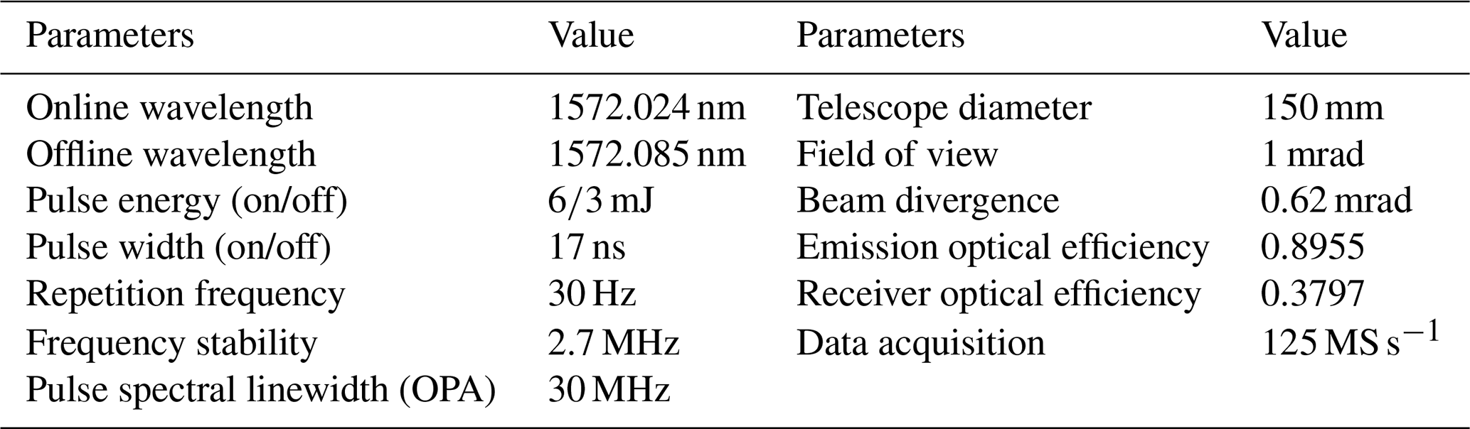
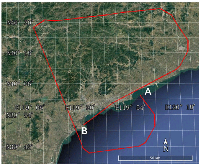
Figure 2Flight trajectory of the flight on 14 March 2019. The starting point of the flight was at A, and the ending point was at B (© Google Earth Pro).
The ACDL consists of a laser transmitter, an instrument control unit, an environmental control unit, and a lidar transceiver subsystem. Figure 1a shows the transceiver system. It mainly included a laser, a telescope, a receiving system, and an APD detector, which were mounted in a pod outside the aircraft. Figure 1b shows the laser frequency monitoring and control system, electronic control system, and the data acquisition system of the equipment. These systems were installed inside the aircraft and armoured optical fibres and cables were used to transmit the information to the instruments in the pod. An inertial navigation system (INS) was also installed to record the attitude information of the aircraft during the flight. The real-time altitude and position information of aircraft were acquired using a Global Positioning System (GPS). Figure 1c shows the Aircraft Integrated Meteorological Measurement System (AIMMS). The AIMMS was installed to measure the atmospheric temperature, pressure, relative humidity, and other meteorological parameters during the flight. Figure 1d shows a commercial instrument (UGGA) that was installed in an unsealed cabin of the aircraft, and a in. Teflon pipe was used to connect it with the external atmosphere. The UGGA used a laser absorption technology known as the off-axis integrated cavity output spectroscopy (ICOS) to measure trace gas concentration in dry mole fraction with a high precision of <0.30 ppm for CO2 and <2 ppb for CH4 (UGGA user manual; model 915-0011; Los Gatos Research, San Jose, CA, USA). More details about the UGGA and ICOS are given in previous studies (Baer et al., 2002; Paul et al., 2001; Sun et al., 2020). Before the flight experiment, the UGGA was calibrated against the standard gas, and the uncertainty was within 0.1 ppm.
2.2 Experimental site
The airborne campaign was conducted from 11–19 March 2019. More details about the flights are given in Table 2. Figure 2 shows the geolocation of the experimental site and path of the flight carried out on 14 March. In order to detect the changing trend of atmospheric CO2 concentration over various types of surfaces, the path of the flight was designed to observe the ocean, urban residential, and mountain areas. The starting point of the flight was at A, and the ending point was at B. The flight path covered a variety of surface types, including the ocean, the mountain, and the urban residential areas. The distribution of the carbon sources and sinks in the study area can be more accurately distinguished through the detection of various surface types. Figure 3 shows the flight altitude and the corresponding surface elevation information during the level flight period. The altitude of the aircraft was measured by the GPS. The height and the ground elevation were measured using the airborne IPDA lidar. The altitude of the horizontal flight of the plane on 14 March was about 6.8 km. Moreover, the altitude information about various types of surfaces is also shown in Fig. 3.

2.3 Datasets
2.3.1 Aircraft data
A variety of data were measured using the aircraft and incorporated into this study. The aircraft data included the ACDL data, in situ data, and the auxiliary data. The in situ CO2 dry-air mole fraction data were measured using the UGGA which was installed in an unsealed cabin of the aircraft. The auxiliary data included the inertial navigational and meteorological data. The inertial navigational data were measured using the INS, and the meteorological data were measured using the AIMMS, which was installed on the aircraft shell. In addition, a colour complementary metal oxide semiconductor (CMOS) camera (model: IDS ui-3360cp-c-hq Rev.2) with a resolution of 2048×1088 pixels was also installed next to the lidar telescope to observe the various types of surfaces. The image sampling rate was 1 Hz. Each picture incorporated the shooting time, and it provided a convenience to find the types of surfaces at different times. The photo filename included the camera date and time, which was synchronized with the other instruments installed on the aircraft.
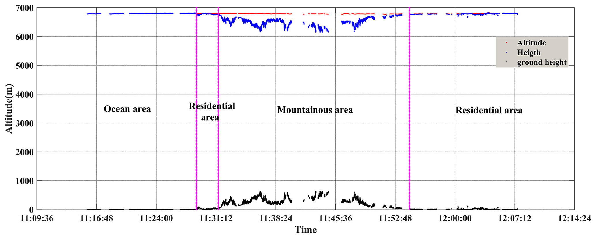
Figure 3Aircraft flight height and corresponding surface elevation on 14 March 2019. The red dots are the altitude of the aircraft measured by the onboard GPS. The blue scatter points represent the distance between the plane and ground measured by lidar. The black scattered points represent the difference between the altitude measured by the GPS and the distance measured by the lidar, and they also represent the surface elevation. The purplish red vertical line is the dividing line for different surface types.
2.3.2 OCO-2 dataset
The Orbiting Carbon Observatory-2 (OCO-2), developed by NASA, is the second satellite after the Greenhouse gases Observing SATellite (GOSAT) to monitoring the CO2 in the atmosphere to get a better understanding of the carbon cycle (Crisp, 2015; Crisp et al., 2008). The main objectives of the mission included measuring atmospheric CO2 with sufficient precision, accuracy, and spatiotemporal resolution required to quantify the CO2 sources and sinks at regional and global scales. The sun-synchronous near-polar satellite included three high-resolution spectrometers simultaneously measuring the reflected sunlight in the near-infrared CO2 at 1.61 and 2.06 µm as well as oxygen at 0.76 µm (Wunch et al., 2017). In this study, the OCO-2 XCO2 version 10r Level 2 Lite product was used.
2.3.3 CarbonTracker dataset
Validation of model measurements against accurate CO2 profiles is also crucial, because the satellite retrieval algorithms require a priori profiles which are generally based on models and in situ data. CarbonTracker is one model widely used by the CO2 community, and the IPDA lidar is an effective tool for high-precision observation of atmospheric CO2. In addition, the measurement range of passive remote sensing is limited, and the model can simulate the situation in a large range. CarbonTracker is an inverse model framework developed by Peters et al. (2004). It combines the two-way nested Transfer Model 5 (TM5) with offline Atmospheric Tracer transfer model and updates the atmospheric CO2 distribution and surface fluxes every year (Krol et al., 2005). It supports high-resolution data at regional level and coarse-resolution data at the global scale. The CarbonTracker provides the global CO2 distribution at 25 pressure levels with a spatial grid resolution of (longitude × latitude) and a temporal resolution of 3 h (Babenhauserheide et al., 2015). The data product CTNRT2020 was used in this study (Jacobson et al., 2020).
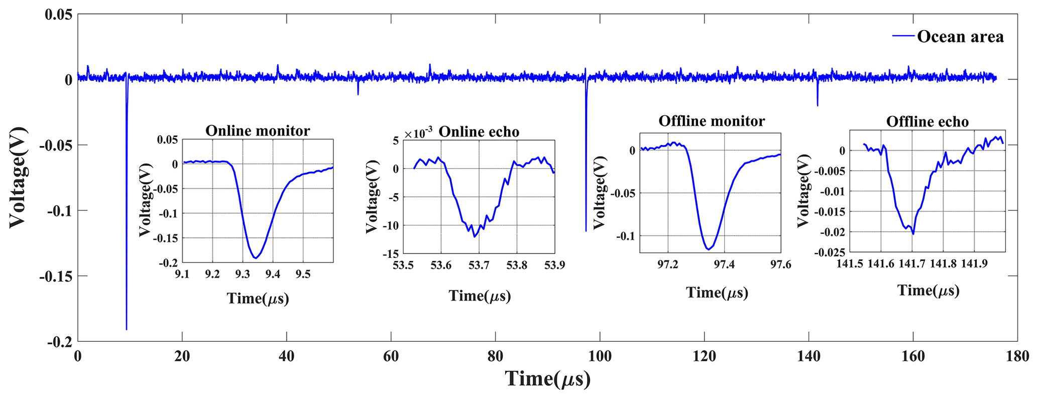
Figure 4Original echo signal of ocean area (total signal and pulse amplification signal). The amplification signals from left to right are online monitor signal, online echo signal, offline monitor signal, and offline echo signal.
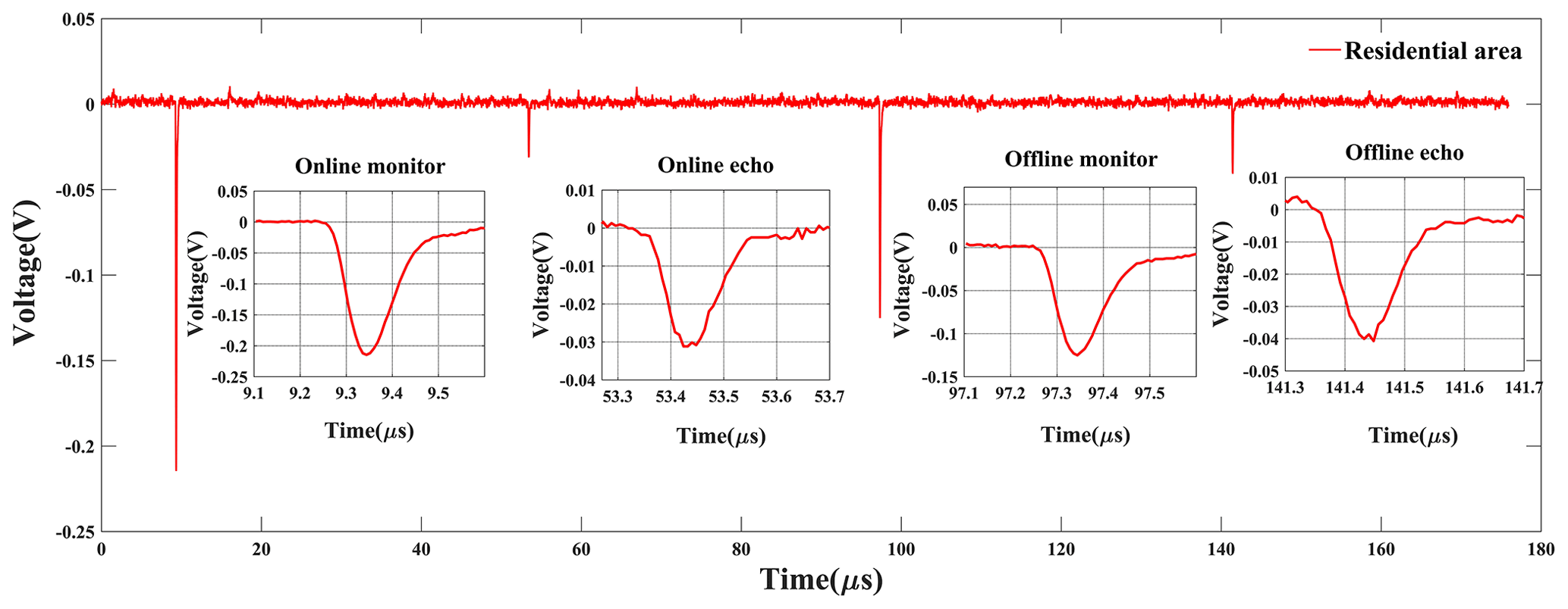
Figure 5Original echo signal of urban residential area (total signal and pulse amplification signal). The amplification signals from left to right are online monitor signal, online echo signal, offline monitor signal, and offline echo signal.
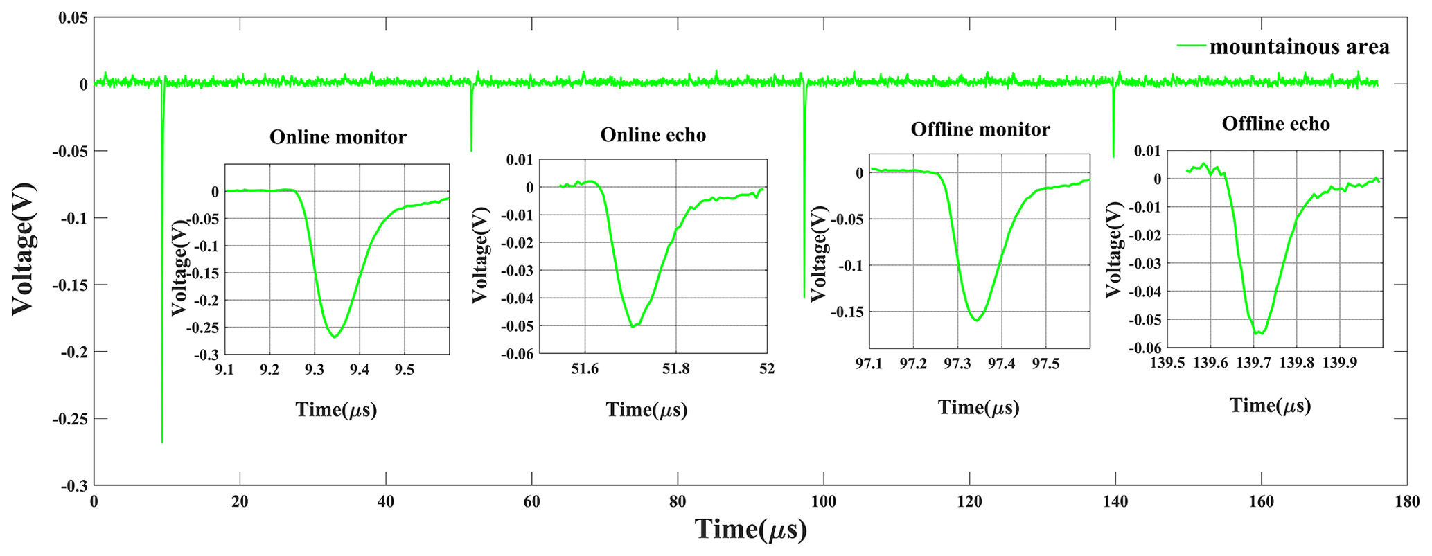
Figure 6Original echo signal of mountain area (total signal and pulse amplification signal). The amplification signals from left to right are online monitor signal, online echo signal, offline monitor signal, and offline echo signal.
2.4 IPDA theory
The ACDL system developed for this study was based on two different wavelengths referred to as the online and the offline wavelengths. The laser pulse of the online wavelength was strongly attenuated, because it was absorbed by the CO2 molecules while propagating through the atmosphere. In contrast, the offline pulse was only weakly attenuated (Zhang et al., 2020). The online and offline wavelengths selected in this study were not affected by molecules other than CO2. Because the online and the offline wavelengths were very close, the difference of scattering and absorption caused by the aerosols and the gas molecules in the atmosphere could be ignored. Therefore, the difference between the two wavelength echo signals was mainly caused by atmospheric CO2. The airborne IPDA lidar equation (Ehret et al., 2008; Refaat et al., 2016) is given in the following:
where Pe is the echo power, λ is the wavelength, ηr is the receiving optical efficiency, Or is the overlap factor, A is the area of the telescope, RG is the height of the surface above sea level, RA is the altitude of the aircraft platform, E is the emission energy of the laser, Δt is the effective pulse width of the echo pulse, ρ∗ is the target reflectivity, is the two-way integral optical depth caused by CO2 (given by Eq. 2 below), and Tm is the atmospheric transmission efficiency. The monitor signals of online and offline pulses are defined as P0(λon) and P0(λoff), respectively. The echo signals of the online and offline pulses are P(λon,R) and P(λoff,R), respectively. The IPDA single-pass differential absorption optical depth (DAOD) of the CO2, , can be expressed as (Refaat et al., 2015):
where is the differential absorption cross section of the online and offline wavelengths, is the molecular density of the CO2, and p and T are pressure and temperature profiles, respectively. When the APD detector receives the signal, it can convert the power into voltage according to Eq. (3) (Zhu et al., 2020):
where Rν (V W−1) represents the voltage response rate of the APD detector, PP is the power of echo signal, and V is the voltage. Within the linear response range of the detector, the voltage response rate is a fixed value Rν which indicates signal power. Using Eq. (3), Eq. (2) can also be expressed as
where V0(λon) and V0(λoff) are the monitor signal voltages of online and offline pulses. V(λon,R) and V(λoff,R) are the echo signal voltages of the online and offline pulses. For the airborne experiment, the vertical path XCO2 (in ppm) can be calculated using the following equations:
where NA is the Avogadro's constant, and R is the gas constant, p(r) and T(r) are the pressure and temperature profiles, respectively. is the dry-air ratio of water vapour, “IWF” represents the integral weight function. IWF can be calculated using the temperature, pressure, and humidity profiles obtained by the AIMMS and the high-resolution transmission molecular absorption (HITRAN) database (Gordon et al., 2017).
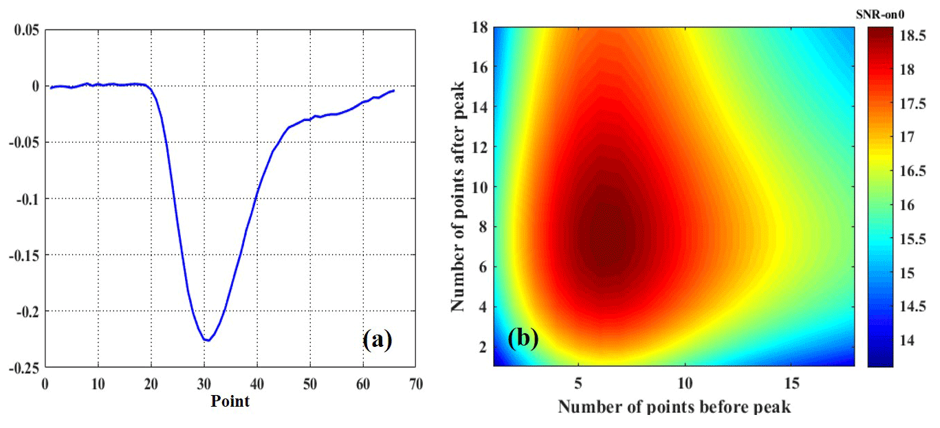
Figure 7(a) Online wavelength monitoring pulse signal. (b) The change of pulse signal-to-noise ratio (SNR) with the number of selected pulse points.
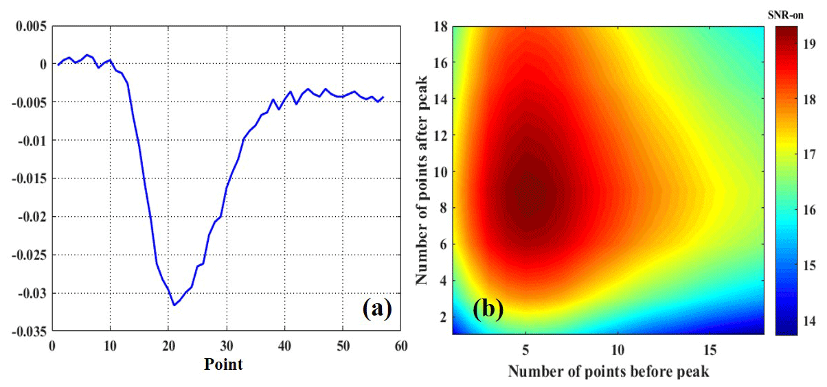
Figure 8(a) Online wavelength echo pulse signal in land area. (b) The change of the SNR of the echo pulse signal in the land area with the number of selected pulse points.
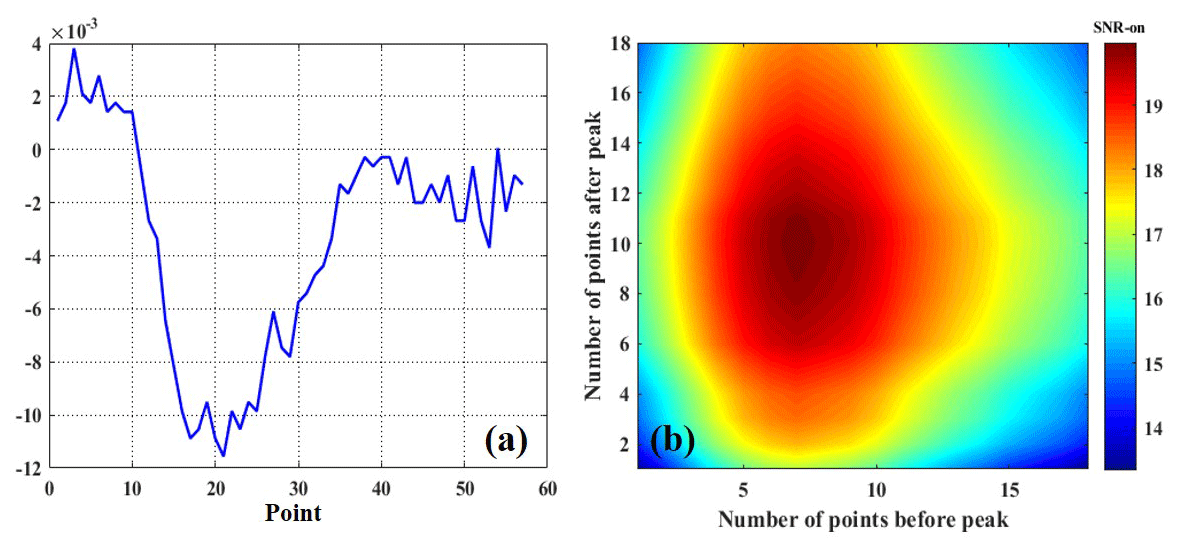
Figure 9(a) Online wavelength echo pulse signal in ocean area. (b) The change of the SNR of the echo pulse signal in the ocean area with the number of selected pulse points.
Zhu et al. (2020) used the matched filter algorithm (MFA) to extract the weak echo signals over the ocean in previous research work. In addition, the differences between the pulse peak method (PPM) and pulse integration method (PIM) were also compared while calculating the DAOD (refer to Eq. 2). The results showed that the SNR and accuracy of PIM were higher than those of the PPM. In this study, the PIM uses the integrated value of the points on the pulse to calculate DAOD. In our experiment, the random noise followed a Gaussian distribution. When the points on the pulse are superimposed, the sum continues following the Gaussian distribution of , where the mean and the variance are given as follows (Zhu et al., 2020; Yoann et al., 2018):
where N is the point number of the pulse, ρl and εl represent the mean and standard deviation, is the value of each point on the pulse, and is the standard deviation of each point. Hence, the empirical estimate of the SNR of the equivalent measurement on the whole averaging window can be written
Therefore, we can choose the number of points on the pulse to improve the SNR of each pulse.
3.1 Original echo signals
The performance of the ACDL system was evaluated by comparing the original echo signals over three different surface types, including the ocean, the mountain, and the urban residential surface types. The original signals of the ACDL over the ocean, urban residential, and mountainous areas are shown in Figs. 4, 5, and 6, respectively, including local amplification of each signal. The amplification signals from left to right are online monitor signal, online echo signal, offline monitor signal, and offline echo signal. In each group of original echo signals, the online and offline monitor signals are fixed at the same position, but the echo signals appear in different positions due to the different heights of the ground surface. The original signals were filtered before use, and the signals whose pulse peak values were not in the linear region of APD were discarded. The echo signals in the ocean area were significantly smaller than those over the residential and the mountain areas. This might be due to the low reflectivity of the ocean, which leads to a reduction of the signal-to-noise ratio (SNR) over the ocean.
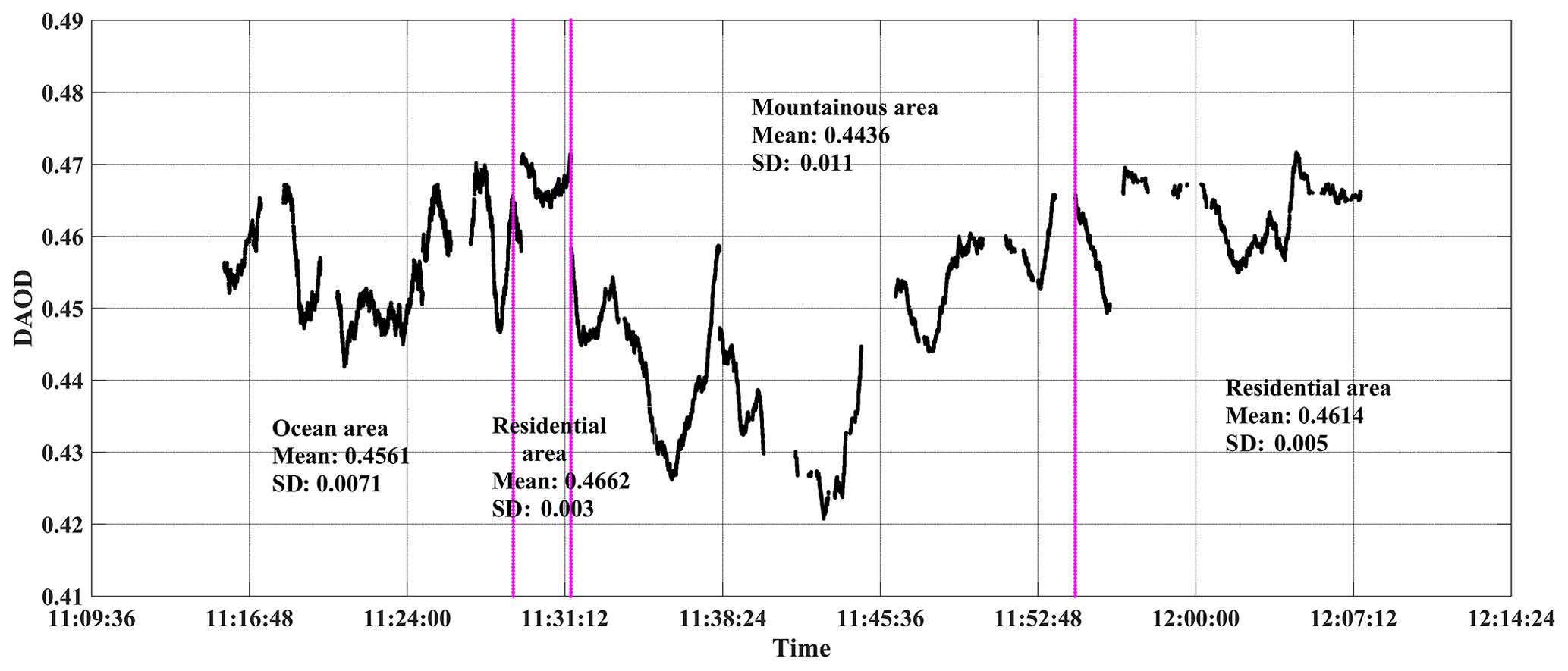
Figure 10DAOD results over ocean areas, urban residential areas and mountain areas on 14 March 2019. The purplish red vertical line represents the boundary of different surface types. The plane passes through the ocean area, urban residential area, mountain area, and urban residential area in turn, which is the same in the following results.

Figure 11IWF results over ocean, urban residential, and mountainous areas on 14 March 2019. The purplish red vertical line represents the boundary of different surface types.
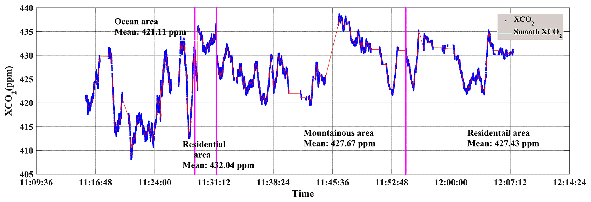
Figure 12XCO2 results over ocean, urban residential, and mountainous areas on 14 March 2019. The purplish red vertical line represents the boundary of different surface types.
3.2 Data processing and inversion results
We can increase the SNR of each pulse by accumulating the number of points on the pulse. Figure 7a shows the online wavelength monitoring signal, and Fig. 7b shows the change of SNR relative to the number of accumulated points taken on the pulse. Figures 8a and 9a show the typical echo signals over the land and the ocean areas. Figures 8b and 9b show the change of SNR relative to the number of accumulated points taken on the pulse over different surface types. For the residential and mountain areas, the SNR was the highest when 5 points were taken before the pulse peak and 9 points were taken after the peak. And for the weak echo signal in the ocean area, the SNR was the highest when 7 points were taken before the pulse peak and 10 points were taken after the peak.
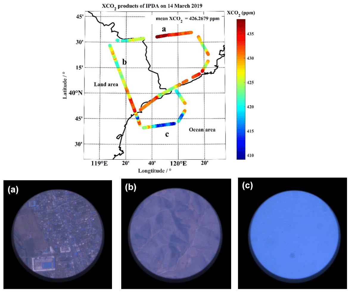
Figure 13XCO2 distribution on the flight trajectory and surface photos of typical areas on 14 March 2019. Among them, (a) represents the urban residential area, (b) represents the mountain area, and (c) represents the ocean area.
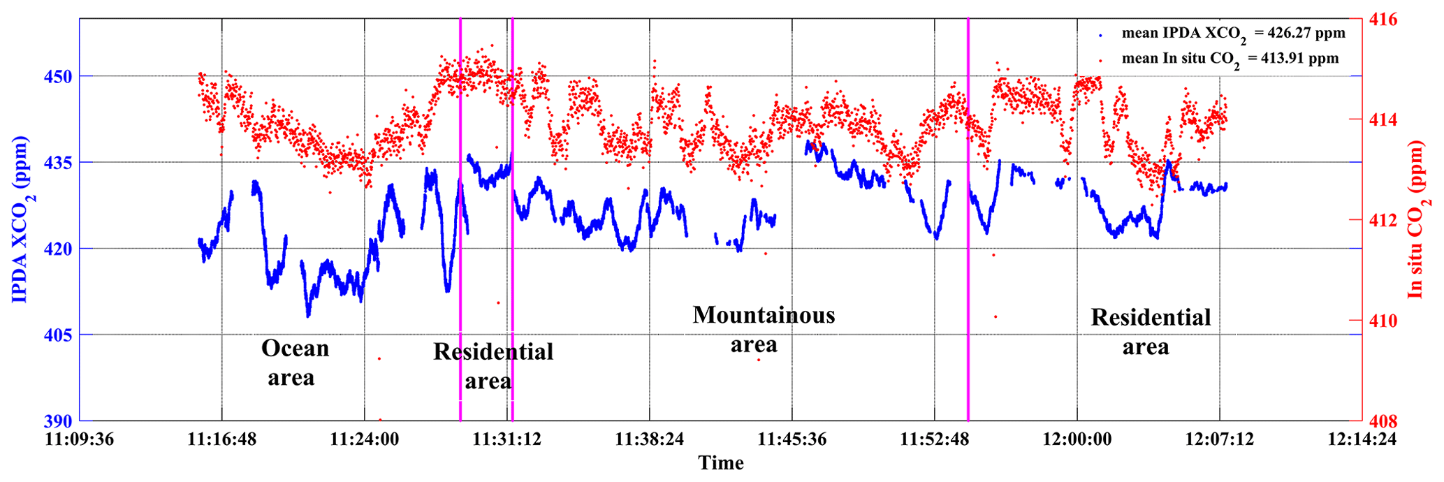
Figure 14XCO2 comparison results of airborne IPDA lidar and lightweight ground radar (LGR) on 14 March 2019. The red scatter is the result of greenhouse gas analyser. The blue scatter is measured by airborne IPDA lidar. The purplish red vertical line represents the boundary of different surface types. The plane passes through the ocean area, urban residential area, mountain area, and urban residential area in turn.
The DAOD results calculated using the IPDA theory are shown in Fig. 10. The DAOD values were smaller over the mountain area; however, no difference was found between the DAOD values of ocean and residential areas. The average DAOD values over ocean, mountainous, and residential areas were 0.46, 0.44, and 0.46, respectively. The results of the IWF and the XCO2 calculated using Eqs. (5) and (6) are shown in Figs. 11 and 12. The average values of the IWF over ocean, mountainous, and residential areas are 1083.26, 1037.05, and 1079.75, respectively. In addition, the standard deviation of the IWF was the smallest for ocean surface and the largest for the mountainous area. The higher standard deviation for mountainous area might be due to the fluctuations in height. Before retrieving the XCO2, the aircraft attitude angle and the Doppler shift were corrected using the inertial navigation data. The XCO2 calculated from the ACDL measurements is shown in Fig. 12. The XCO2 is the largest over residential areas and the smallest over ocean. The largest XCO2 over the urban residential areas might be attributed to the strong anthropogenic emissions (Mustafa et al., 2020), and the water body is generally a sink of the CO2. The average values of XCO2 over ocean, mountainous, and residential areas were 421.11, 427.67, and 432.04 ppm, respectively. Correspondingly, the standard deviation of XCO2 over ocean, mountainous, and residential areas were 1.24, 0.58, and 0.74 (20 s averaged), respectively. The distribution of XCO2 on the flight trajectory and the surface photos captured using the installed coloured CMOS camera are shown in Fig. 13.
3.3 In situ measurement results
The XCO2 measured by the IPDA lidar is a distance average value, which is different from the measured value of in situ instrument at aircraft altitude. Therefore, it is unreasonable to directly compare the two measurement results. This paper only compares the long-term change trend of XCO2 measured by the IPDA lidar system with the CO2 volume mixing ratio measured by UGGA, which can indirectly evaluate the working performance of IPDA lidar. Figure 14 shows the comparison of the XCO2 calculated from the ACDL measurements with the dry-air mole fraction of CO2 measured using the UGGA. Both of the datasets show a good agreement by exhibiting a similar variation trend. The results from the two datasets also show that the volume mixing ratio of atmospheric CO2 is highest over the residential area and the lowest over ocean surface. The average value of XCO2 obtained by the ACDL calculations was 426.27 ppm, and the average value of CO2 mole fraction obtained by the UGGA measurements was 413.91 ppm. Moreover, the standard deviation of the UGGA observations was smaller than that of the ACDL measurements, and this might be due to the different working principles of the two instruments. The ACDL measures the weighted average concentrations at different altitudes. However, the UGGA measures the CO2 value at the aircraft location.
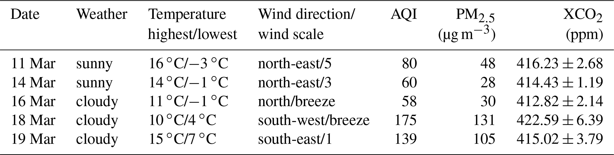
In this study, the in situ observations measured using the UGGA were also analysed for several days. The vertical profiles of atmospheric CO2 were measured using the UGGA during spiral and the descent of the aircraft, and the results are shown in Fig. 15. The data recorded below 0.5 km were discarded because of sudden spikes due to slowing down of the aircraft and the associated sudden pressure changes. Figure 15 shows that the atmospheric CO2 volume mixing ratio is largest near the ground, and it decreases gradually with the progression in altitude. This might be due to the weak photosynthesis as the plants are in dormant stage during winter in northeast China (Mustafa et al., 2021). Moreover, northeast China is also a source of carbon due to heating and industrial activities, which also contributes significantly to atmospheric CO2 (Shan et al., 1997). In addition, the CO2 concentrations at different altitudes were the highest on 18 March. This could be caused by the weather conditions and pollution levels. Table 3 shows the weather report released by the Qinhuangdao meteorological station on each day of the flight.
Table 3The weather report released by the Qinhuangdao Meteorological Bureau on each flight day.
The AOD values measured using various instruments on each flight day are shown Fig. 16, and the results show that the AOD was the largest on 18 March. The highest CO2 concentration on 18 March was likely caused by the higher pollution levels. A ground station was arranged in the flight area to verify the airborne results. A micropulse lidar (MPL) was installed at the Funing ground station to monitor the change of local pollutants and the boundary layer. The change of pollutants and the boundary layer in Funing ground station during the flight test on 18 March is shown in Fig. 17. The dry-air mole fraction of CO2 reaches its maximum value at about 1.4 km on 18 March (Fig. 15). This might be due to the fact that the height of the boundary layer was about 1.5 km on 18 March (Fig. 17), and the pollutants and the greenhouse gases cannot escape through the boundary layer.

Figure 15CO2 concentration profile results measured by the greenhouse gas analyser during aircraft descending flight on different dates. The blue solid line is the result on 11 March. The black solid line is the result for 14 March. The purple solid line is the result for 16 March. The solid red line is the result for 18 March. The green solid line is the result of 19 March.

Figure 16Aerosol optical depth results on different dates. The blue scatter points are measured by the sun photometer of Funing ground station. The black scatter points are the measurement results of the airborne lidar 532 nm channel. The red scatter points are the measurement results of Moderate Resolution Imaging Spectroradiometer (MODIS).
3.4 OCO-2 measurement results
During this flight experiment, the OCO-2 passed over the flight area on 16 March and the observations over the study area are shown in Fig. 18. The solid red line in Fig. 18a is the flight path of the aircraft. The yellow marker point is the position of the suborbital point of the OCO-2 trajectory in the flight area. Figure 18b shows the XCO2 results detected by OCO-2. Figure 18c shows the corresponding standard deviation production of OCO-2. As can be seen from Fig. 18a, OCO-2 observations covered both ocean and land surfaces. Due to the fast flight speed of the satellite, the data time period falling in the study area was from 12:57:25 to 12:57:38 UTC. A quality flag was applied to the satellite dataset, and the cloud-contaminated retrievals were removed. In the flight area, there is little difference between the values of XCO2 measured by OCO-2 over land and ocean areas. The average value of XCO2 over land area is 414.28 ± 0.81 ppm and that over ocean area is 414.23 ± 0.55 ppm. However, due to the uneven distribution of CO2 volume mixing ratio in the land area, the standard deviation of XCO2 products over the land area is larger than that over the ocean. The XCO2 measured by OCO-2 varied from 401.66 to 418.80 ppm, with an average of 414.25 ± 0.62 ppm.
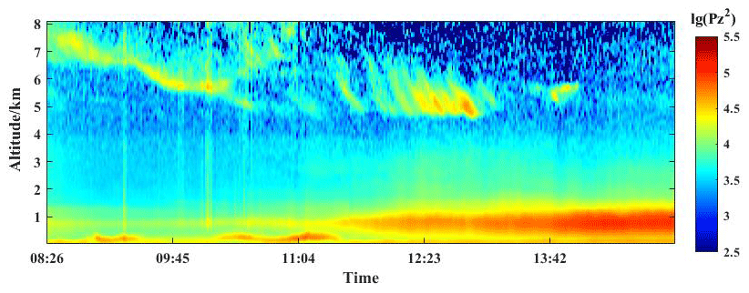
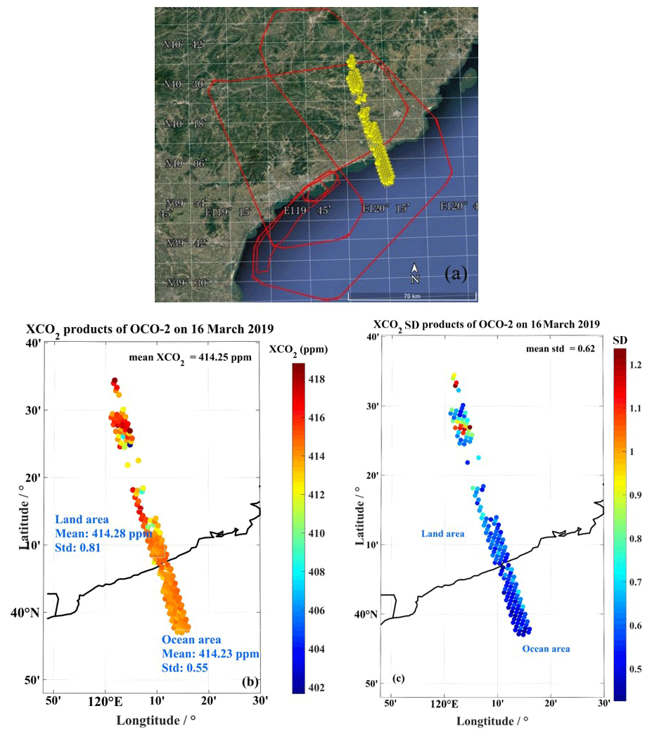
Figure 18Orbit and detection results of OCO-2 satellite on 16 March. The solid red line in (a) is the flight path of the aircraft. The yellow marker point is the position of the suborbital point of the OCO-2 trajectory in the flight area (© Google Earth Pro). Panel (b) shows the XCO2 results detected by OCO-2. Panel (c) shows the corresponding standard deviation.

Figure 19CO2 volume mixing ratio profile comparison results of airborne greenhouse gas analyser and OCO-2 satellite, CarbonTracker model. Panel (a) is the vertical structure of CO2 volume mixing ratio on 14 March. Panel (b) shows the vertical structure of CO2 volume mixing ratio on 16 March. Panel (c) shows the vertical structure of CO2 volume mixing ratio on 19 March. The red error bars represent the inversion result of OCO-2. The blue error bars represent the measurement result of the airborne greenhouse gas analyser. The black solid line is the result of CarbonTracker model.
3.5 Vertical profile comparison of CO2 concentration
The measurement results of the airborne greenhouse gas analyser were compared with those of OCO-2 inversion and CarbonTracker model, which is a global carbon cycle data assimilation system. The comparison results are shown in Fig. 19. The CarbonTracker dataset was interpolated into the location of the experimental site. During the flight campaigns, the OCO-2 satellite passed over the flight area on 16 March. Therefore, the data results of OCO-2 on 16 March were compared with those of CarbonTracker and in situ data on 14, 16, and 19 March , respectively. As can be seen from the detection results in Fig. 19, the structural change of CO2 concentration with height can be roughly divided into two parts. From the ground to the height of 4 km and above 4 km. Below 4 km, the detection results of OCO-2, airborne greenhouse gas analyser, and CarbonTracker model show a similar decreasing of CO2 concentration value with the increase of altitude, but the values are different. The difference between the average values of CO2 concentration obtained by the OCO-2 and the airborne greenhouse gas analyser below 4 km on 14, 16, and 19 March were −1.3, 0.79, and 1.3 ppm, respectively. These three methods can well detect that the land in north-east China was the source of CO2 in March. The results by the airborne greenhouse gas analyser and CarbonTracker are more obvious than OCO-2. On 19 March, CO2 concentration measured by the airborne greenhouse gas analyser decreased from 430.3 ppm at 0.34 km to 413.09 ppm at 3.18 km. The computed results of CarbonTracker decrease from 429.75 ppm at 0.59 km to 415.7 ppm at 2.68 km. The CO2 concentration result of OCO-2 decreased from 414.55 ppm on the ground to 412.39 ppm at 3.02 km. When the altitude is higher than 4 km, the CO2 concentration is almost constant. This might be due to the stability of the atmosphere above.
In this study, a 1.57 µm double-pulsed airborne IPDA lidar was developed for atmospheric CO2 monitoring. The airborne experiment using the newly developed instrument was carried out during 11–19 March 2019 over Shanhaiguan, China. The IPDA lidar was installed on a research aircraft with some other instrument including a commercial CO2-monitoring UGGA, an AIMMS, an INS, and a coloured CMOS camera. The flight path passed across various types of surfaces including ocean, mountain, and residential areas. From the original signals obtained by the IPDA lidar, the echo signals over the ocean area were smaller than those over the mountain and the residential areas. In order to process the echo signal with low SNR over the ocean, the PIM method was used to calculate DAOD. The data obtained by airborne IPDA lidar on 14 March was processed and analysed. The results showed that the XCO2 over the ocean surface was the smallest, with an average value of 421.11 ± 1.24 ppm, and that over residential area was the largest, with an average value of 432.04 ± 0.74 ppm. The average XCO2 value over the mountainous area was 427.67 ± 0.58 ppm. Moreover, the dry-air mole fraction of CO2 measured by UGGA was also analysed for several days, and the results showed that the CO2 volume mixing ratio was largest on 18 March, which was the most polluted day during the entire flight campaign. The UGGA CO2 volume mixing ratio was compared with the XCO2 calculated using the IPDA lidar measurements, and both of the datasets showed a good agreement by exhibiting a similar variation. In addition, the vertical profiles of CO2 were also measured using UGGA and compared with OCO-2 and the CarbonTracker CO2 datasets. The CO2 volume mixing ratio from the CarbonTracker was larger than the dry-air mole fraction of CO2 measured using the UGGA. The atmospheric CO2 volume mixing ratio was the highest near the ground and it decreased gradually with the progression in altitude. Below 4 km, the detection results of OCO-2, airborne greenhouse gas analyser and CarbonTracker model show a same decreasing of CO2 volume mixing ratio value with the increase of altitude but the values are different. The difference between the average values of CO2 volume mixing ratio obtained by the OCO-2 and the airborne greenhouse gas analyser below 4 km on 14, 16, and 19 March were −1.3, 0.79, and 1.3 ppm, respectively. These three methods can well detect that the land in north-east China was the source of CO2 in March. This change result of airborne greenhouse gas analyser and CarbonTracker is more obvious than OCO-2. On 19 March, CO2 volume mixing ratio measured by the airborne greenhouse gas analyser decreased from 430.3 ppm at 0.34 km to 413.09 ppm at 3.18 km. The computed results of CarbonTracker decrease from 429.75 ppm at 0.59 km to 415.7 ppm at 2.68 km. The CO2 volume mixing ratio result of OCO-2 decreased from 414.55 ppm on the ground to 412.39 ppm at 3.02 km. When the altitude is higher than 4 km, the CO2 volume mixing ratio is almost constant. This might be due to the stability of the atmosphere above.
Data used in this study are available from the corresponding author upon request (18262602365@163.com).
QW and SZ carried out the flight experiment, and QW processed the data results. FM provided the satellite and model data as well as analysis methods, and FM modified the grammar and format of the whole manuscript. LB guided the writing of the article. JL and WC guided the flight experiment.
The authors declare that they have no conflict of interest.
Publisher's note: Copernicus Publications remains neutral with regard to jurisdictional claims in published maps and institutional affiliations.
The authors acknowledge the support of the Shanghai Institute of Satellite Engineering for conducting the experiment. The authors thank the Funing Meteorological Bureau for providing a ground station for the experiment. The authors acknowledge the efforts of NASA to provide the OCO-2 data products. These data were produced by the OCO-2 project at the Jet Propulsion Laboratory, California Institute of Technology, and obtained from the OCO-2 data archive maintained at the NASA Goddard Earth Science Data and Information Services Center. The authors also acknowledge NOAA Earth System Research Laboratory for their data products. The second author (Farhan Mustafa) is highly grateful to the China Scholarship Council (CSC) and the NUIST for granting the fellowship and providing the required support.
This research has been supported by the National Natural Science Foundation of China (NSFC) (42175145) and Shanghai Aerospace Science and Technology Innovation Fund (SAST 2019-045).
This paper was edited by Alexander Kokhanovsky and reviewed by two anonymous referees.
Abshire, J., Ramanathan, A., Riris, H., Mao, J., Allan, G., Hasselbrack, W., Weaver, C., and Browell, E.: Airborne Measurements of CO2 Column Concentration and Range Using a Pulsed Direct-Detection IPDA Lidar, Remote Sens., 6, 443–469, https://doi.org/10.3390/rs6010443, 2013.
Abshire, J. B., Ramanathan, A. K., Riris, H., Allan, G. R., Sun, X., Hasselbrack, W. E., Mao, J., Wu, S., Chen, J., Numata, K., Kawa, S. R., Yang, M. Y. M., and DiGangi, J.: Airborne measurements of CO2 column concentrations made with a pulsed IPDA lidar using a multiple-wavelength-locked laser and HgCdTe APD detector, Atmos. Meas. Tech., 11, 2001–2025, https://doi.org/10.5194/amt-11-2001-2018, 2018.
Amediek, A., Ehret, G., Fix, A., Wirth, M., Büdenbender, C., Quatrevalet, M., Kiemle, C., and Gerbig, C.: CHARM-F – a new airborne integrated-path differential-absorption lidar for carbon dioxide and methane observations: measurement performance and quantification of strong point source emissions, Appl. Opt., 56, 5182, https://doi.org/10.1364/AO.56.005182, 2017.
Araki, M., Morino, I., MacHida, T., Sawa, Y., Matsueda, H., Ohyama, H., Yokota, T., and Uchino, O.: CO2 column-averaged volume mixing ratio derived over Tsukuba from measurements by commercial airlines, Atmos. Chem. Phys., 10, 7659–7667, https://doi.org/10.5194/acp-10-7659-2010, 2010.
Babenhauserheide, A., Basu, S., Houweling, S., Peters, W., and Butz, A.: Comparing the CarbonTracker and TM5-4DVar data assimilation systems for CO2 surface flux inversions, Atmos. Chem. Phys., 15, 9747–9763, https://doi.org/10.5194/acp-15-9747-2015, 2015.
Baer, D. S., Paul, J. B., Gupta, M., and O'Keefe, A.: Sensitive absorption measurements in the near-infrared region using off-axis integrated-cavity-output spectroscopy, Appl. Phys. B, 75, 261–265, https://doi.org/10.1007/s00340-002-0971-z, 2002.
Ballantyne, A. P., Alden, C. B., Miller, J. B., Trans, P. P., and White, J. W. C.: Increase in observed net carbon dioxide uptake by land and oceans during the past 50 years, Nature, 488, 70–73, https://doi.org/10.1038/nature11299, 2012.
Crisp, D.: Measuring atmospheric carbon dioxide from space with the Orbiting Carbon Observatory-2 (OCO-2), In Earth Observing Systems, International Society for Optics and Photonics, Washington, DC, USA, Vol. 9607, 2015.
Crisp, D., Miller, C. E., and DeCola, P. L.: NASA Orbiting Carbon Observatory: measuring the column averaged carbon dioxide mole fraction from space, J. Appl. Remote Sens., 2, 1–14, https://doi.org/10.1117/1.2898457, 2008.
Crisp, D., Fisher, B. M., O'Dell, C., Frankenberg, C., Basilio, R., Bösch, H., Brown, L. R., Castano, R., Connor, B., Deutscher, N. M., Eldering, A., Griffith, D., Gunson, M., Kuze, A., Mandrake, L., McDuffie, J., Messerschmidt, J., Miller, C. E., Morino, I., Natraj, V., Notholt, J., O'Brien, D. M., Oyafuso, F., Polonsky, I., Robinson, J., Salawitch, R., Sherlock, V., Smyth, M., Suto, H., Taylor, T. E., Thompson, D. R., Wennberg, P. O., Wunch, D., and Yung, Y. L.: The ACOS CO2 retrieval algorithm – Part II: Global XCO2 data characterization, Atmos. Meas. Tech., 5, 687–707, https://doi.org/10.5194/amt-5-687-2012, 2012.
Dlugokencky, T. P. (Ed.): Trends in Atmospheric Carbon Dioxide, Noaa/Esrl, available at: http://www.esrl.noaa.gov/gmd/ccgg/trends/global.ht (last access: 3 May 2020), 2016.
Du, J., Zhu, Y., Li, S., Zhang, J., Sun, Y., Zang, H., Liu, D., Ma, X., Bi, D., Liu, J., Zhu, X., and Chen, W.: Double-pulse 157 µm integrated path differential absorption lidar ground validation for atmospheric carbon dioxide measurement, Appl. Opt., 56, 7053, https://doi.org/10.1364/AO.56.007053, 2017.
Ehret, G., Kiemle, C., Wirth, M., Amediek, A., Fix, A., and Houweling, S.: Space-borne remote sensing of CO2, CH4, and N2O by integrated path differential absorption lidar: a sensitivity analysis, Appl. Phys. B, 90, 593–608, https://doi.org/10.1007/s00340-007-2892-3, 2008.
Gong, Y., Bu, L., Yang, B., and Mustafa, F.: High Repetition Rate Mid-Infrared Differential Absorption Lidar for Atmospheric Pollution Detection, Sensors, 20, 2211, https://doi.org/10.3390/s20082211, 2020.
Gordon, I. E., Rothman, L. S., Hill, C., Kochanov, R. V., Tan, Y., Bernath, P. F., Birk, M., Boudon, V., Campargue, A., Chance, K. V., Drouin, B. J., Flaud, J.-M., Gamache, R. R., Hodges, J. T., Jacquemart, D., Perevalov, V. I., Perrin, A., Shine, K. P., Smith, M.-A. H., Tennyson, J., Toon, G. C., Tran, H., Tyuterev, V. G., Barbe, A., Császár, A. G., Devi, V. M., Furtenbacher, T., Harrison, J. J., Hartmann, J.-M., Jolly, A., Johnson, T. J., Karman, T., Kleiner, I., Kyuberis, A. A., Loos, J., Lyulin, O. M., Massie, S. T., Mikhailenko, S. N., Moazzen-Ahmadi, N., Müller, H. S. P., Naumenko, O. V., Nikitin, A. V., Polyansky, O. L., Rey, M., Rotger, M., Sharpe, S. W., Sung, K., Starikova, E., Tashkun, S. A., Auwera, J. Vander, Wagner, G., Wilzewski, J., Wcisło, P., Yu, S., and Zak, E. J.: The HITRAN2016 molecular spectroscopic database, J. Quant. Spectrosc. Ra., 203, 3–69, https://doi.org/10.1016/j.jqsrt.2017.06.038, 2017.
Hedelius, J. K., Parker, H., Wunch, D., Roehl, C. M., Viatte, C., Newman, S., Toon, G. C., Podolske, J. R., Hillyard, P. W., Iraci, L. T., Dubey, M. K., and Wennberg, P. O.: Intercomparability of XCO2 and XCH4 from the United States TCCON sites, Atmos. Meas. Tech., 10, 1481–1493, https://doi.org/10.5194/amt-10-1481-2017, 2017.
Hungershoefer, K., Peylin, P., Chevallier, F., Rayner, P., Klonecki, A., Houweling, S., and Marshall, J.: Evaluation of various observing systems for the global monitoring of CO2 surface fluxes, Atmos. Chem. Phys., 10, 10503–10520, https://doi.org/10.5194/acp-10-10503-2010, 2010.
Jacobson, A. R., Schuldt, K. N., Miller, J. B., Tans, P., Andrews, A., Mund, J., Aalto, T., Bakwin, P., Bergamaschi, P., Biraud, S. C., Chen, H., Colomb, A., Conil, S., Cristofanelli, P., Davis, K., Delmotte, M., DiGangi, J. P., Dlugokencky, E., Emmenegger, L., Fischer, M. L., Hatakka, J., Heliasz, M., Hermanssen, O., Holst, J., Jaffe, D., Karion, A., Keronen, P., Kominkova, K., Kubistin, D., Laurent, O., Laurila, T., Lee, J., Lehner, I., Leuenberger, M., Lindauer, M., Löfvenius, M. O., Lopez, M., Mammarella, I., Manca, G., Marek, M. V., Marklund, P., Martin, M. Y., McKain, K., Miller, C. E., Mölder, M., Myhre, C. L., Pichon, J. M., Plass-Dölmer, C., Ramonet, M., Scheeren, B., Schumacher, M., Sloop, C. D., Steinbacher, M., Sweeney, C., Thoning, K., Tørseth, K., Turnbull, J., Viner, B., Vitkova, G., Wekker, S. De, Weyrauch, D., and Worthy, D.: CarbonTracker Near Real-Time, CT-NRT.v2020-1, https://doi.org/10.25925/RCHH-MS75, 2020.
Kawa, S. R., Mao, J., Abshire, J. B., Collatz, G. J., Sun, X., and Weaver, C. J.: Simulation studies for a space-based CO2 lidar mission, Tellus B, 62, 759–769, https://doi.org/10.1111/j.1600-0889.2010.00486.x, 2010.
Kiel, M., O'Dell, C. W., Fisher, B., Eldering, A., Nassar, R., MacDonald, C. G., and Wennberg, P. O.: How bias correction goes wrong: measurement of X affected by erroneous surface pressure estimates, Atmos. Meas. Tech., 12, 2241–2259, https://doi.org/10.5194/amt-12-2241-2019, 2019.
Kong, Y., Chen, B., and Measho, S.: Spatio-temporal consistency evaluation of XCO2 retrievals from GOSAT and OCO-2 based on TCCON and model data for joint utilization in carbon cycle research, Atmosphere (Basel), 10, 1–23, https://doi.org/10.3390/atmos10070354, 2019.
Krol, M., Houweling, S., Bregman, B., van den Broek, M., Segers, A., van Velthoven, P., Peters, W., Dentener, F., and Bergamaschi, P.: The two-way nested global chemistry-transport zoom model TM5: algorithm and applications, Atmos. Chem. Phys., 5, 417–432, https://doi.org/10.5194/acp-5-417-2005, 2005.
Kulawik, S., Wunch, D., O'Dell, C., Frankenberg, C., Reuter, M., Oda, T., Chevallier, F., Sherlock, V., Buchwitz, M., Osterman, G., Miller, C. E., Wennberg, P. O., Griffith, D., Morino, I., Dubey, M. K., Deutscher, N. M., Notholt, J., Hase, F., Warneke, T., Sussmann, R., Robinson, J., Strong, K., Schneider, M., De Mazière, M., Shiomi, K., Feist, D. G., Iraci, L. T., and Wolf, J.: Consistent evaluation of ACOS-GOSAT, BESD-SCIAMACHY, CarbonTracker, and MACC through comparisons to TCCON, Atmos. Meas. Tech., 9, 683–709, https://doi.org/10.5194/amt-9-683-2016, 2016.
Lei, L., Zhong, H., He, Z., Cai, B., Yang, S., Wu, C., Zeng, Z., Liu, L., and Zhang, B.: Assessment of atmospheric CO2 concentration enhancement from anthropogenic emissions based on satellite observations, Kexue Tongbao, Chin. Sci. Bull., 62, 2941–2950, https://doi.org/10.1360/N972016-01316, 2017.
Liang, A., Gong, W., Han, G., and Xiang, C.: Comparison of satellite-observed XCO2 from GOSAT, OCO-2, and ground-based TCCON, Remote Sens., 9, 1–26, https://doi.org/10.3390/rs9101033, 2017.
Lindqvist, H., O'Dell, C. W., Basu, S., Boesch, H., Chevallier, F., Deutscher, N., Feng, L., Fisher, B., Hase, F., Inoue, M., Kivi, R., Morino, I., Palmer, P. I., Parker, R., Schneider, M., Sussmann, R., and Yoshida, Y.: Does GOSAT capture the true seasonal cycle of carbon dioxide?, Atmos. Chem. Phys., 15, 13023–13040, https://doi.org/10.5194/acp-15-13023-2015, 2015.
Mao, J., Ramanathan, A., Abshire, J. B., Kawa, S. R., Riris, H., Allan, G. R., Rodriguez, M., Hasselbrack, W. E., Sun, X., Numata, K., Chen, J., Choi, Y., and Yang, M. Y. M.: Airborne lidar reflectance measurements at 1.57 µm in support of the A-SCOPE mission for atmospheric CO2, Atmos. Meas. Tech., 11, 127–140, https://doi.org/10.5194/amt-11-127-2018, 2018a.
Mao, J., Ramanathan, A., Abshire, J. B., Kawa, S. R., Riris, H., Allan, G. R., Rodriguez, M., Hasselbrack, W. E., Sun, X., Numata, K., Chen, J., Choi, Y., and Yang, M. Y. M.: Measurement of atmospheric CO2 column concentrations to cloud tops with a pulsed multi-wavelength airborne lidar, Atmos. Meas. Tech., 11, 127–140, https://doi.org/10.5194/amt-11-127-2018, 2018b.
Mendonca, J., Strong, K., Wunch, D., Toon, G. C., Long, D. A., Hodges, J. T., Sironneau, V. T., and Franklin, J. E.: Using a speed-dependent Voigt line shape to retrieve O2 from Total Carbon Column Observing Network solar spectra to improve measurements of XCO2, Atmos. Meas. Tech., 12, 35–50, https://doi.org/10.5194/amt-12-35-2019, 2019.
Mustafa, F., Bu, L., Wang, Q., Ali, M. A., Bilal, M., Shahzaman, M., and Qiu, Z.: Multi-year comparison of CO2 concentration from NOAA carbon tracker reanalysis model with data from GOSAT and OCO-2 over Asia, Remote Sens., 12, 2498–2519, https://doi.org/10.3390/RS12152498, 2020.
Mustafa, F., Wang, H., Bu, L., Wang, Q., Shahzaman, M., Bilal, M., Zhou, M., Iqbal, R., Aslam, R. W., Ali, M. A., and Qiu, Z.: Validation of GOSAT and OCO-2 against In Situ Aircraft Measurements and Comparison with CarbonTracker and GEOS-Chem over Qinhuangdao, China, Remote Sens., 13, 899–914, https://doi.org/10.3390/rs13050899, 2021.
O'Dell, C. W., Connor, B., Bösch, H., O'Brien, D., Frankenberg, C., Castano, R., Christi, M., Eldering, D., Fisher, B., Gunson, M., McDuffie, J., Miller, C. E., Natraj, V., Oyafuso, F., Polonsky, I., Smyth, M., Taylor, T., Toon, G. C., Wennberg, P. O., and Wunch, D.: The ACOS CO2 retrieval algorithm – Part 1: Description and validation against synthetic observations, Atmos. Meas. Tech., 5, 99–121, https://doi.org/10.5194/amt-5-99-2012, 2012.
Paul, J. B., Lapson, L., and Anderson, J. G.: Ultrasensitive absorption spectroscopy with a high-finesse optical cavity and off-axis alignment, Appl. Opt., 40, 4904–4910, https://doi.org/10.1364/AO.40.004904, 2001.
Peters, W., Krol, M. C., Dlugokencky, E. J., Dentener, F. J., Bergamaschi, P., Dutton, G., Velthoven, P. V., Miller, J. B., Bruhwiler, L., and Tan, P. P.: Toward regional-scale modeling using the two-way nested global model TM5: Characterization of transport using SF6, J. Geophys. Res., 109, D19314, https://doi.org/10.1029/2004JD005020, 2004.
Refaat, T. F., Singh, U. N., Yu, J., Petros, M., Ismail, S., Kavaya, M. J., and Davis, K. J.: Evaluation of an airborne triple-pulsed 2 µm IPDA lidar for simultaneous and independent atmospheric water vapor and carbon dioxide measurements, Appl. Opt., 54, 1387, https://doi.org/10.1364/AO.54.001387, 2015.
Refaat, T. F., Singh, U. N., Yu, J., Petros, M., Remus, R., and Ismail, S.: Double-pulse 2-µm integrated path differential absorption lidar airborne validation for atmospheric carbon dioxide measurement, Appl. Opt., 55, 4232, https://doi.org/10.1364/AO.55.004232, 2016.
Santer, B. D., Painter, J. F., Bonfils, C., Mears, C. A., Solomon, S., Wigley, T. M. L., Gleckler, P. J., Schmidt, G. A., Doutriaux, C., Gillett, N. P., Taylor, K. E., Thorne, P. W., and Wentz, F. J.: Human and natural influences on the changing thermal structure of the atmosphere, P. Natl. Acad. Sci. USA, 110, 17235–17240, https://doi.org/10.1073/pnas.1305332110, 2013.
Schultz, M. G., Akimoto, H., Bottenheim, J., Buchmann, B., Galbally, I. E., Gilge, S., Helmig, D., Koide, H., Lewis, A. C., Novelli, P. C., Plass-Dölmer, C., Ryerson, T. B., Steinbacher, M., Steinbrecher, R., Tarasova, O., Tørseth, K., Thouret, V., and Zellweger, C.: The global atmosphere watch reactive gases measurement network, Elementa, 3, 1–23, https://doi.org/10.12952/journal.elementa.000067, 2015.
Shan, Y., Guan, D., Zheng, H., Ou, J., Li, Y., Meng, J., Mi, Z., Liu, Z., and Zhang, Q.: China CO2 emission accounts 1997–2015, Sci. Data, 5, 1–14, 1997.
Stocker, B. D., Roth, R., Joos, F., Spahni, R., Steinacher, M., Zaehle, S., Bouwman, L., Xu-Ri, and Prentice, I. C.: Multiple greenhouse-gas feedbacks from the land biosphere under future climate change scenarios, Nat. Clim. Change, 3, 666–672, https://doi.org/10.1038/nclimate1864, 2013.
Sun, X., Duan, M., Gao, Y., Han, R., Ji, D., Zhang, W., Chen, N., Xia, X., Liu, H., and Huo, Y.: In situ measurement of CO2 and CH4 from aircraft over northeast China and comparison with OCO-2 data, Atmos. Meas. Tech., 13, 3595–3607, https://doi.org/10.5194/amt-13-3595-2020, 2020.
Tellier, Y., Pierangelo, C., Wirth, M., Gibert, F., and Marnas, F.: Averaging bias correction for the future space-borne methane IPDA lidar mission MERLIN, Atmos. Meas. Tech., 11, 5865–5884, https://doi.org/10.5194/amt-11-5865-2018, 2018.
UNFCC: The United Nations Framework Convention on Climate Change, Review of European Community and International Environmental Law, 1, 270–277, 2006.
Wunch, D., Wennberg, P. O., Osterman, G., Fisher, B., Naylor, B., Roehl, M. C., O'Dell, C., Mandrake, L., Viatte, C., Kiel, M., Griffith, D. W. T., Deutscher, N. M., Velazco, V. A., Notholt, J., Warneke, T., Petri, C., De Maziere, M., Sha, M. K., Sussmann, R., Rettinger, M., Pollard, D., Robinson, J., Morino, I., Uchino, O., Hase, F., Blumenstock, T., Feist, D. G., Arnold, S. G., Strong, K., Mendonca, J., Kivi, R., Heikkinen, P., Iraci, L., Podolske, J., Hillyard, P., Kawakami, S., Dubey, M. K., Parker, H. A., Sepulveda, E., García, O. E., Te, Y., Jeseck, P., Gunson, M. R., Crisp, D., and Eldering, A.: Comparisons of the Orbiting Carbon Observatory-2 (OCO-2) XCO2 measurements with TCCON, Atmos. Meas. Tech., 10, 2209–2238, https://doi.org/10.5194/amt-10-2209-2017, 2017.
Xie, J., Huang, X., Bu, L., Zhang, H., Mustafa, F., and Chu, C.: Detection of water cloud microphysical properties using multi-scattering polarization lidar, Curr. Opt. Photonics, 4, 174–185, https://doi.org/10.3807/COPP.2020.4.3.174, 2020.
Yang, S., Lei, L., Zeng, Z., He, Z., and Zhong, H.: An Assessment of Anthropogenic CO2 Emissions by Satellite-Based Observations in China, Sensors (Basel), 19, 1118, https://doi.org/10.3390/s19051118, 2019.
Tellier, Y., Pierangelo, C., Wirth, M., Gibert, F., and Marnas, F.: Averaging bias correction for the future space-borne methane IPDA lidar mission MERLIN, Atmos. Meas. Tech., 11, 5865–5884, https://doi.org/10.5194/amt-11-5865-2018, 2018.
Yokota, T., Yoshida, Y., Eguchi, N., Ota, Y., Tanaka, T., Watanabe, H., and Maksyutov, S.: Global Concentrations of CO2 and CH4 Retrieved from GOSAT: First Preliminary Results, Scientific Online Letters on the Atmosphere, 5, 160–163, 2009.
Yu, J., Petros, M., Singh, U. N., Refaat, T. F., Reithmaier, K., Remus, R. G., and Johnson, W.: An Airborne 2-µm Double-Pulsed Direct-Detection Lidar Instrument for Atmospheric CO2 Column Measurements, J. Atmos. Ocean. Technol., 34, 385–400, https://doi.org/10.1175/JTECH-D-16-0112.1, 2017.
Zhang, X., Wang, F., Wang, W., Huang, F., Chen, B., Gao, L., Wang, S., Yan, H., Ye, H., Si, F., Hong, J., Li, X., Cao, Q., Che, H., and Li, Z.: The development and application of satellite remote sensing for atmospheric compositions in China, Atmos. Res., 245, 105056, https://doi.org/10.1016/j.atmosres.2020.105056, 2020.
Zhu, Y., Yang, J., Chen, X., Zhu, X., Zhang, J., Li, S., Sun, Y., Hou, X., Bi, D., Bu, L., Zhang, Y., Liu, J., and Chen, W.: Airborne Validation Experiment of 1.57-µm Double-Pulse IPDA LIDAR for Atmospheric Carbon Dioxide Measurement, Remote Sens., 12, 1999, https://doi.org/10.3390/rs12121999, 2020.