the Creative Commons Attribution 4.0 License.
the Creative Commons Attribution 4.0 License.
 | 26 Oct 2021
The “ideal” spectrograph for atmospheric observations
Ulrich Platt
Thomas Wagner
Thomas Leisner
Spectroscopy of scattered sunlight in the near-UV to near-IR spectral ranges has proven to be an extremely useful tool for the analysis of atmospheric trace gas distributions. A central parameter for the achievable sensitivity and spatial resolution of spectroscopic instruments is the étendue (product of aperture angle and entrance area) of the spectrograph, which is at the heart of the instrument. The étendue of an instrument can be enhanced by (1) upscaling all instrument dimensions or (2) by changing the instrument F number, (3) by increasing the entrance area, or (4) by operating many instruments (of identical design) in parallel. The étendue can be enhanced by (in principle) arbitrary factors by options (1) and (4); the effect of options (2) and (3) is limited.
We present some new ideas and considerations of how instruments for the spectroscopic determination of atmospheric gases could be optimized using new possibilities in spectrograph design and manufacturing. Particular emphasis is on arrays of massively parallel instruments for observations using scattered sunlight. Such arrays can reduce size and weight of instruments by orders of magnitude while preserving spectral resolution and light throughput. We also discuss the optimal size of individual spectrographs in a spectrograph array and give examples of spectrograph systems for use on a (low Earth orbit) satellite, including one with sub-kilometre ground pixel size.
- Article
(4195 KB) - Full-text XML
- BibTeX
- EndNote


Spectroscopy of scattered sunlight in the near-UV to near-IR spectral ranges has proven to be an extremely useful tool for the analysis of atmospheric trace gas distributions (see, for example, Platt and Stutz, 2008). Applications include the determination of trace gas vertical profiles by MultiAXis Differential Optical Absorption Spectroscopy (MAX-DOAS; see, for example, Hönninger and Platt, 2002; Sinreich et al., 2005), observation of volcanic gases, for example, by the Network for the Observation of Volcanic and Atmospheric Change (NOVAC; see, for example, Galle et al., 2010), and satellite observation of global trace gas distributions (e.g. Burrows et al., 1999; Levelt et al., 2006; Veefkind et al., 2012).
Central components of these instruments are moderate-resolution (typical spectral resolution, , is around several hundred) grating spectrographs. In all practical applications (except, perhaps observations with direct sunlight), the measurement precision (i.e. the attainable signal-to-noise ratio, SNR) and thus the detection limit of such spectrographs are ultimately limited by the number of photons detected during a given time interval, i.e. by the spectrographs' light throughput (see, for example, Platt and Stutz, 2008). As for most spectroscopic instruments, the light throughput of a spectrograph is basically determined by its étendue.
For example, consider a satellite spectrograph like that used in the GOME-1/2 (Burrows et al., 1996, 1999; Munroe et al., 2016), SCIAMACHY (Burrows and Chance, 1991; Bovensmann et al., 1999), OMI (Levelt et al., 2006; Dobber et al., 2006), or TROPOMI (Sentinel 5P mission, Veefkind et al., 2012) instruments. These instruments feature ground pixel sizes of 320×40 (GOME-1), 80×40 (GOME-2), 60×30 (SCIAMACHY), 13×24 (OMI), and down to 5.5×3.5 km2 (TROPOMI); there is a clear evolution towards smaller ground pixel sizes (mainly driven by increase of the online storage capacities and downlink rates), allowing smaller and smaller structures to be monitored in the distribution of trace gases in the atmosphere. For instance, the GOME-2 ground pixel more or less covers an entire megacity, while the TROPOMI ground pixel size allows structures and hotspots within a city to be identified. It appears clearly desirable to further shrink the ground pixel size, for instance in order to fully resolve industrial or volcanic emission plumes or to identify small-scale events. From a high spatial resolution (of, for example, 1 km×1 km or better) in the spectral range 270–500 nm, not only would the NO2 retrievals benefit, but also the retrieval of SO2, BrO, IO, OClO, HCHO, O4, glyoxal, and water vapour. This improvement in spatial resolution can be accomplished for instance by using a longer focal length telescope. When the F number (ratio of focal length f to diameter of the optics, D) of the telescope is preserved, the étendue of the instrument per pixel will not change. Unfortunately, there is a problem: many more pixels have to be observed. Assuming a 2600 km swath of the instrument (required to obtain global coverage from a sun-synchronous low Earth orbit within 1 d) at a satellite velocity of ≈7 km s−1, an area of about 18 200 km2 has to be observed every second. Dividing this area into 5.5×3.5 km2 pixels (as TROPOMI does for the near-UV and Vis bands) requires 743 pixels, while 18 200 pixels of 1×1 km2 would be required, i.e. about 24 times more.
At a given spectrograph size, fewer photoelectrons per pixel would be recorded, leading to higher photoelectron shot noise, since the SNR is inversely proportional to the square root of the total number nP of photoelectrons recorded by a detector pixel (in modern detectors, read-out noise and dark current noise are usually negligible compared to the photon shot noise; see, for example, Platt and Stutz, 2008). This geometrical relationship cannot be compensated for by longer exposure times τexp, since the orbital velocity vsat of the satellite is fixed. In fact, quite the opposite is true: the along-track dimension of the ground pixels is given by vsat⋅τexp (neglecting the along-track extension of the instantaneous field of view). Thus, smaller along-track extensions of ground pixels require reduced exposure times. A lower SNR of the intensity directly translates into a reduced SNR of the trace gas column density derived from the recorded spectra. Up to now, this decrease in SNR at higher spatial resolution was partly compensated by higher trace gas column densities seen by smaller ground pixels. This effect is due to the “smearing out” of column-density hotspots by larger ground pixels. However, future instruments with even smaller ground pixel sizes, with spatial extensions comparable to or smaller than the extension of trace gas hotspots, will benefit less or not at all from this effect. Therefore, it is important that future, high-spatial-resolution instruments will exhibit higher étendue per pixel.
In the following, we discuss the design options to maximize the étendue of a spectrograph or spectrograph array. We present new ways to reduce volume and mass of spectrographs for environmental remote sensing applications while retaining spectral resolution and light throughput. Alternatively, in the same manner, the light throughput can be greatly enhanced without increasing volume and mass of the instrument. Our considerations are largely theoretical and are based on first principles, like the well-known scaling laws of nature as, for example, spelled out by Haldane (1927). However, we neither intend to present a plan for actually realizing an array of spectrographs, nor are our considerations restricted to satellite instruments. We also note here that massively parallel optics is used in other areas of science, e.g. in astronomy (see, for instance, Schilling, 2021).
Typically DOAS instruments use small- to medium-size (focal length f=50 to 500 mm) grating spectrographs with spectral resolutions in the 0.1 to 1 nm range (see, for example, Platt and Stutz, 2008).
2.1 Typical design of a DOAS spectrograph
Frequently the Czerny–Turner (Czerny and Turner, 1930) design is employed as sketched in Fig. 1a. However, other designs, e.g. imaging grating spectrographs, are also in use (see, for example, General et al., 2014, or Ferlemann et al., 2000; see Fig. 1b). The considerations presented in the following are largely independent of the particular spectrograph design. We also note that modern spectrographs using focal plane detector arrays, which simultaneously record the intensity of the entire spectrum of interest, enjoy the “multiplex advantage” over a scanning spectrograph. Therefore, using interferometers, which may (see Fellgett, 1949) or may not (see Barducci et al., 2011) feature a multiplex advantage, instead of grating spectrographs will probably not lead to better light throughput per se.
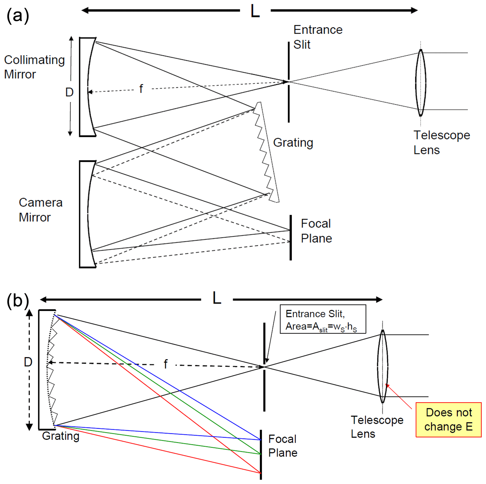
Figure 1Typical design of DOAS spectrographs with telescope: (a) (symmetrical) Czerny–Turner spectrograph plus telescope. The size of the spectrograph L is largely determined by the focal length f. Its F number is given by the ratio of focal length f and diameter of the optics, D. The étendue is a function of the F number and proportional to the slit area, which is a product of slit width (wS, extension in dispersion direction) and slit height (hS). (b) Imaging spectrographs with a concave grating; L and the F number (see Eq. 6) are given in the same way as for the Czerny–Turner spectrograph. Note that in both cases the étendue of the spectrograph is the same as that of the spectrograph + telescope lens.
2.2 The spectrograph light throughput and noise
We assume a spectrograph entrance slit with width wS and height hS; thus an area (see Fig. 1); also we assume the aperture solid angle to be Ω. The étendue E of the instrument is thus given by
Let us consider a modern compact spectrograph (as, for example, described by General et al., 2014) with an entrance area (i.e. width×height of the spectrograph entrance slit) of AS≈0.6 mm2 at an F number of 4 (see definition of the F number in Eq. 6 below), equivalent to Ω≈0.05 sr. The total étendue (product of free entrance area and solid angle of acceptance of the entrance optics) of such an instrument would be about 0.03 mm2 sr (or m2 sr; see also Sect. 2.3 below).
We further assume the spectrograph to be equipped with a linear detector array, with pixels of width wPix and a pixel “height” (pixel dimension perpendicular to the dispersion direction) sufficient to collect all light. The spectral interval δλ covered by a detector pixel will then be given by the spectrograph's linear dispersion and wPix as . Note that the spectral interval of a pixel is typically smaller than the spectral resolution of the instrument by a factor of 2 to 6.
Measurements of the clear-sky photon flux F at 320 nm indicate F≈20 (e.g. Blumenthaler et al., 1996) at a 30∘ observation elevation angle and at a solar zenith angle of 68∘.
The corresponding number of photons registered per pixel and second by such a spectrograph is given by (see, for example, Stutz and Platt, 2008, or Platt et al., 2015)
where WPhot denotes the energy of a single photon (about J for λ=320 nm). Assuming a typical δλ≈0.1 nm and the values for E and F from above results in about 108 photons per pixel and second.
2.3 Improving the spectrograph light throughput
In the following, we investigate measures to improve the spectrograph light throughput.
In principle improving the quality of the optics (reflectivity of the mirrors, grating efficiency, etc.) will increase the light throughput; however, typically the instruments are rather optimized in this respect, and the possible gain due to these measures is rather small (say of the order of 2). Moreover, improved optics can be combined with all measures to be described below. Therefore we restrict our discussion to other measures.
Overall, there are the following options (which to some extent can be combined):
-
Scale the size of the spectrograph, i.e. all three dimension lengths L1, height L2, and width L3, and thus the entrance slit area, while keeping the acceptance angle (i.e. the spectrograph F number) constant. We refer to this option as “spectrograph size scaling”.
-
Increase the étendue while keeping some dimensions of the spectrograph constant. For instance, scale the acceptance angle (i.e. the F number) of the spectrograph while keeping its entrance area AS constant. We refer to this option as “spectrograph F number scaling”.
-
Alternatively, the entrance area AS may be scaled up while retaining the F number. For instance the slit height hS could be made larger.
-
Scale the number of spectrographs; i.e. use multiple spectrographs with given étendue in parallel, and electronically combine the resulting spectra. The latter point will be discussed in more detail below.
Below we have a closer look at the effects of the above options for the improvement of light throughput – while keeping the resolution constant – on spectrograph volume and mass.
2.3.1 Spectrograph size scaling
We now investigate how the spectrograph light throughput changes when the spectrograph size is scaled up or down while keeping the acceptance angle (i.e. the spectrograph F number) constant. We assume that the typical dimension of the spectrograph L (e.g. the length of the housing) is scaled from its initial value L0 to some other value in such a way that all other dimensions (including entrance slit dimensions) are scaled proportional to L as sketched in Fig. 2; i.e. L1 is scaled to Γ⋅L1, L2 is scaled to Γ⋅L2, L3 is scaled to Γ⋅L3, wS0 is scaled to Γ⋅wS0, and hS0 is scaled to Γ⋅hS0.
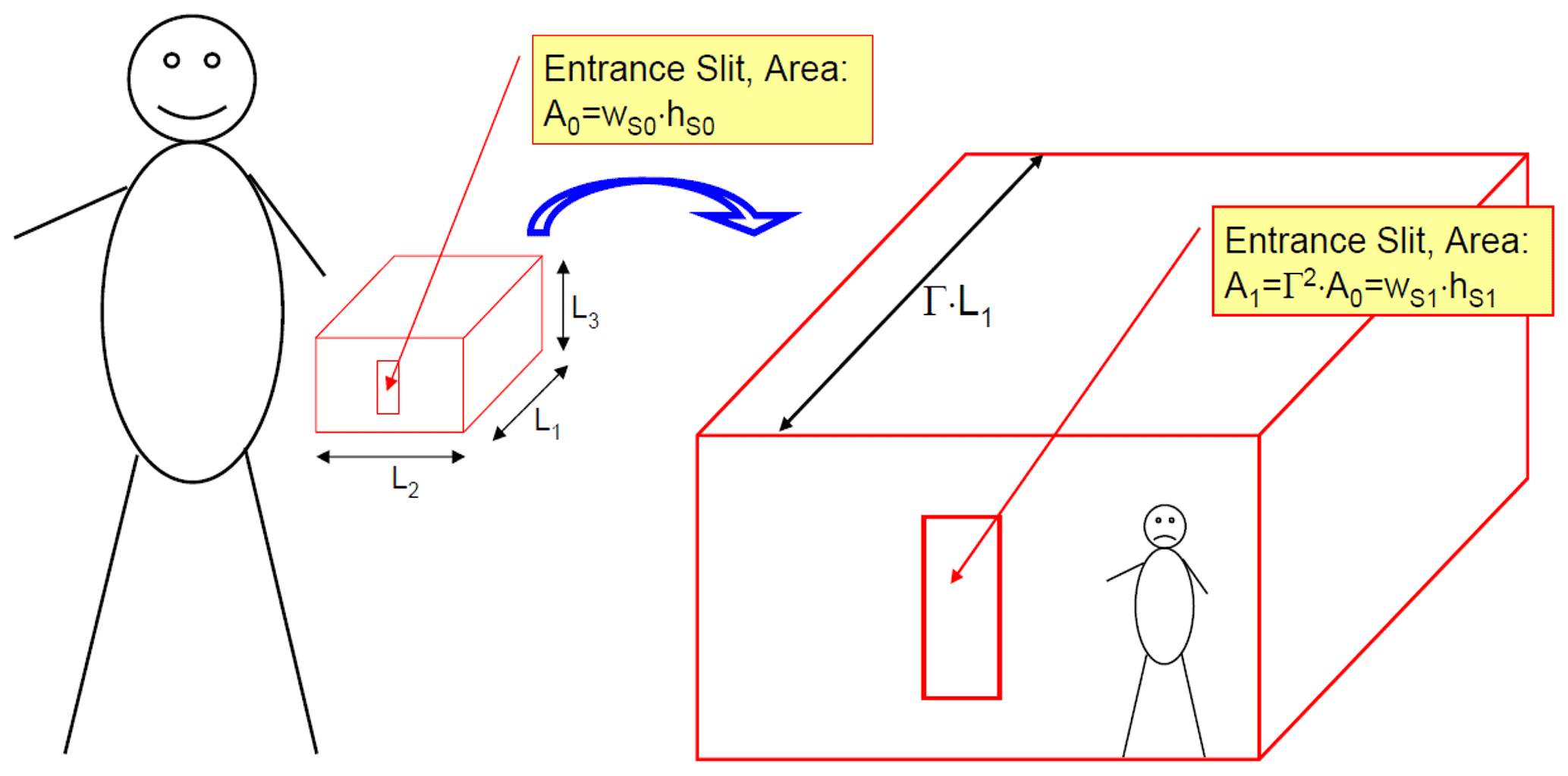
Figure 2Scaling a spectrograph with the linear scaling factor Γ at constant aspect ratio, i.e. preserving the ratio between the dimensions L1, L2, and L3 as well as between L1 and wS (wS, slit extension in dispersion direction) and hS. For instance, a spectrograph scaled up by a factor of 10 in its linear dimensions would feature a 100 times higher étendue but have 1000 times the mass.
Thus, the aperture solid angle Ω (and F number) will stay constant; however the étendue E(L) will change from its initial value E0=E(L0), since the area AS of the entrance slit will scale according to
However, volume and mass of the spectrograph scale with L3; i.e.
Thus, mass and volume of a spectrograph scale with its light throughput (as measured by the Étendue) as
Note that in the case of satellite instruments, the size of the entrance slit will influence the instantaneous ground pixel size; for details see Sect. 4.1.
2.3.2 Scale spectrograph acceptance angle
Another option for improving the spectrograph light throughput is increasing its acceptance aperture angle Ω by changing the aspect ratio of the spectrograph. Here, frequently the F number (F) of the spectrograph is quoted, which is related to the diameter D of the optics and its focal length f. F is defined as (see Fig. 1)
For moderate F numbers, the following (approximate) relationship between F and Ω holds:
Typical DOAS spectrographs have F numbers between 4 and 6. For satellite instruments in the literature, no F numbers for the actual spectrograph are given; however they can be estimated from the F number for the telescope (for TROPOMI ≈9.5; see Babic et al., 2019 and Table 2) to be around F≈2.
The corresponding aperture solid angles range from Ω≈0.2 (F=2) to Ω≈0.02 (F=6).
Table 1Summary of scaling options for the improvement of spectrograph light throughput at a given spectral resolution.
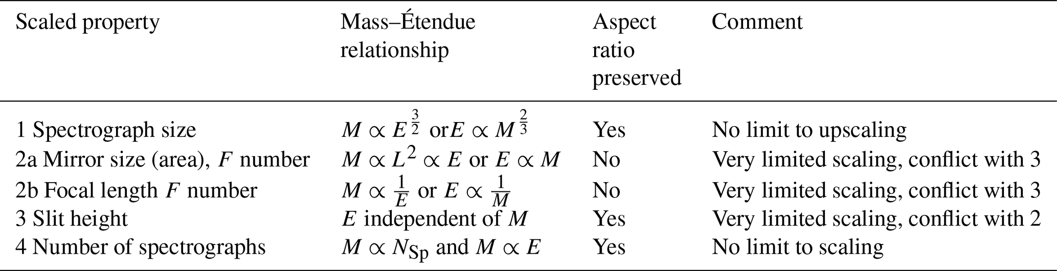
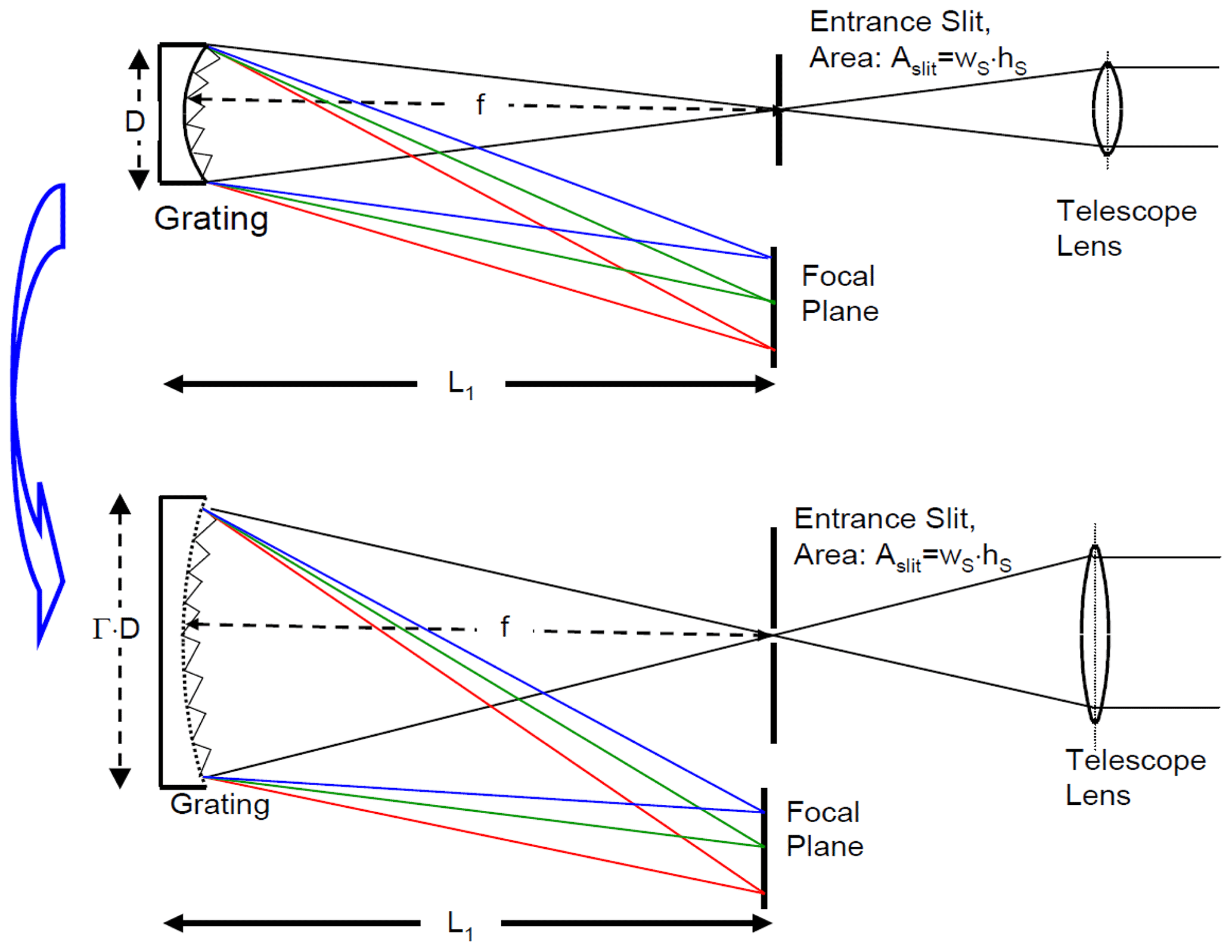
Figure 3Scaling the spectrograph (plus telescope) F number, option a: scale size (i.e. diameter) of the optics D with the linear scaling factor Γ, while focal length and slit dimensions, i.e. slit width (extension in dispersion direction) and slit height (extension perpendicular to the dispersion direction), are preserved.
There are two options (see cases 2a and 2b in Table 1):
- a.
The F number – for given entrance slit dimensions – could be increased by increasing the area of the mirror (i.e. D2) as given in Eq. (7). This would require to scale D to Γ⋅D, L2 to Γ⋅L2 and L3 to Γ⋅L3 as sketched in Fig. 3, while the focal length f and the dimensions of the entrance slit would be unchanged. Since the volume of the spectrograph would scale as (not L3 as in the case of spectrograph size scaling; see Sect. 2.3.1 and Eq. 5). Thus, its mass would scale as
- b.
Alternatively the focal length f could be changed, i.e. from f0 to , as sketched in Fig. 4. Since changes in f also change the spectral resolution, the width of the entrance slit wS would have to be changed proportional to f (wS∝f, i.e. ). Therefore, the étendue would change as (rather than in the case of constant entrance slit dimensions, as suggested by Eq. 7). In this case, the spectrograph mass would scale as
This leads to the interesting conclusion that a spectrograph with given spectral resolution but higher étendue would actually be lighter than one with smaller étendue, if the transformation is done by scaling the focal length of the instrument and the width of the entrance slit. While it appears that the two above ways to change the spectrograph aspect ratio are very different and give opposite results, it is easy to show that they are actually the same and can be further broken down into two steps. This is shown in more detail in Appendix A.
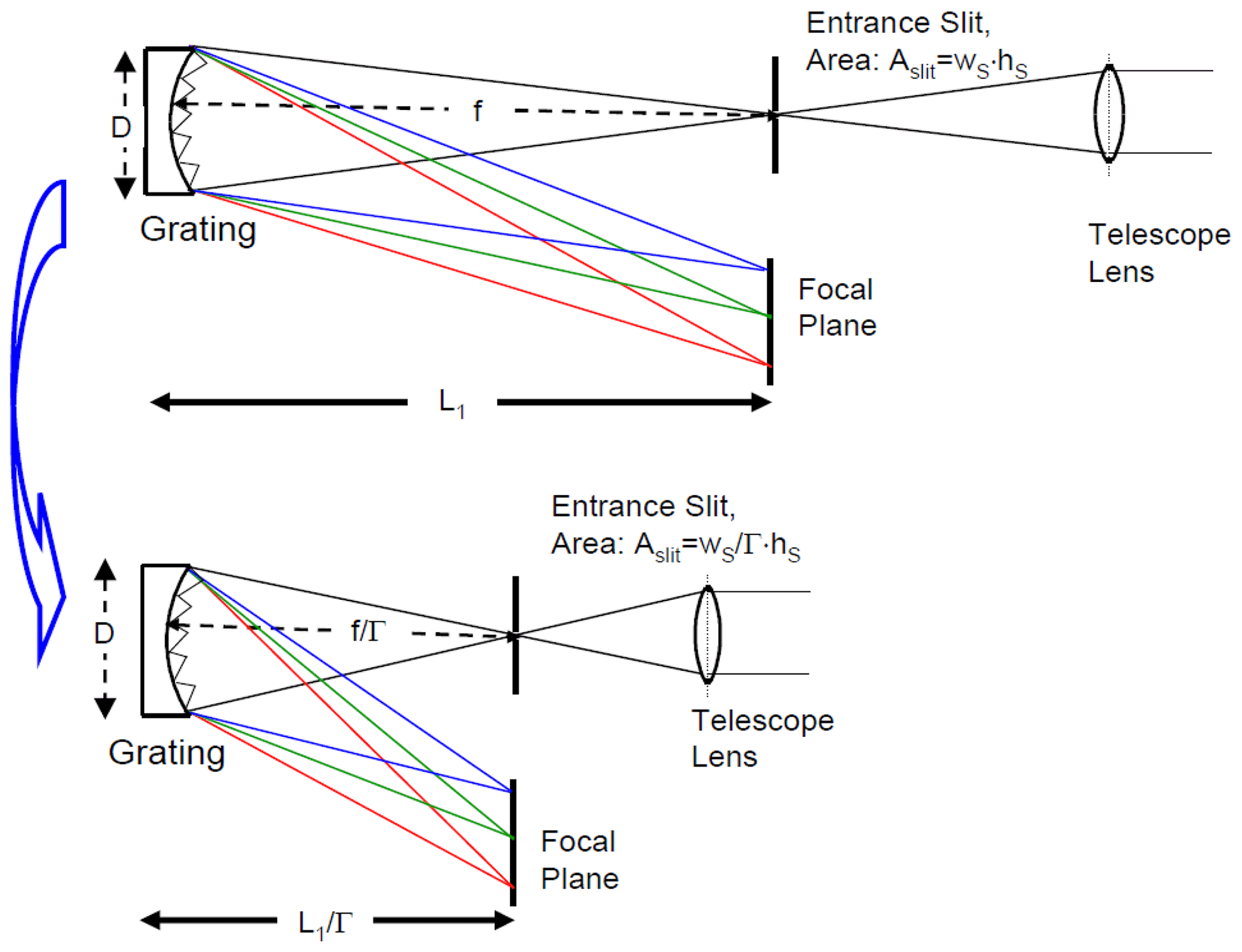
Figure 4Scaling the spectrograph (plus telescope) F number, option b: change focal length and entrance slit dimensions (width) while diameter of the optics is preserved. Scaling down the focal length requires narrowing the entrance slit width (reduction of wS) by the same factor in order to preserve the spectral resolution.
However, the amount of upscaling the étendue that can actually be applied to a spectrograph in this way is extremely limited due to rapid growth of the imaging errors (e.g. astigmatism) of the optics. Also, the aperture solid angle Ω of the instrument can usually not exceed (actually not even approach) 2π. Since the entrance area is kept constant (case a) or even shrinks (case b) with upscaling Ω, the gain in étendue is limited.
2.3.3 Scale spectrograph entrance area
The spectrograph entrance area A is given by (see, for example, Fig. 1). However, widening the entrance slit (i.e. making wS bigger) at a given spectrograph focal length (and grating grove spacing; see below) would reduce the spectral resolution, so it is not an option. On the other hand, the slit height does not seem to have an immediate effect on the resolution; thus increasing hS (at an otherwise unchanged spectrograph) would appear to be a measure to improve the étendue. However, there is an increasing amount of image distortion due to astigmatism when hS is made bigger, which will also degrade the spectral resolution. A quantification of the problem was given by Fastie (1952), who found an empirical relationship between astigmatism as defined as the difference Δf between the sagittal focal length and the meridional focal length (see also Kuhn et al., 2021):
The width of the astigmatic spread is then . This corresponds to an additional width of the image Δw (in dispersion direction) due to the astigmatism: . With the grating clear aperture b (approximately equal to the spectrograph aperture diameter D), we obtain
If we allow an additional width (and the corresponding slight degradation in spectral resolution), we obtain
From this consideration, it becomes clear that the slit height is limited; for instance, for a typical F=4 spectrograph with wS=50 µm, one obtains mm. Moreover, smaller F numbers would require less slit height in order to retain the desired resolution. This relationship severely limits the gain in étendue possible by either reducing the F number or increasing the slit height.
It should be noted that reducing the grating groove spacing g (all other spectrograph parameters being kept unchanged) can also be a way to improve the étendue of a spectrograph, at least if the spectral range covered by the instrument is not a high priority. A smaller groove spacing g will enhance the linear dispersion of the instrument approximately proportional to ; thus the width of the entrance slit wS (and its height hS; see Eq. 12 above) can be made proportionally wider, which should enhance the étendue approximately as . This measure is clearly limited, since the grating groove spacing should not be smaller than the wavelength, and usually, gratings are selected to have a groove spacing close to this limit.
There is one little discussed possibility to further enhance the groove density, which relies on “immersing” the grating in a transparent (for the wavelength range to be measured) material with an index of refraction n>1 (see, for example, Larsson and Neuhaus, 1968).
Thus, the grating will see not the vacuum (or air) wavelength λ0 but rather λ0/n, which can be considerably shorter, allowing for proportionally higher groove densities. Possible materials for the UV (and visible) range could be quartz (n≈1.5–1.6), sapphire (n≈1.6–1.8), or diamond (n≈2.4–2.6). In the short-wave infrared range, crystalline silicon (n≈3.5) was successfully used (van Amerongen et al., 2010).
2.3.4 Scale number of spectrographs
In a number of applications (e.g. for the satellite instruments GOME, SCIAMACHY, GOME-2, OMI, and TROPOMI; see Introduction), the total spectral range is divided among several spectrographs, each covering part of the total wavelength interval of the instrument. However, in all DOAS applications for each spectral interval, only a single spectrograph is used.
Up to now, the possibility of using a number of NSp spectrographs (for simplicity assumed to be identical in design, each with Étendue E0) in parallel and co-adding their spectra was not considered, although this option clearly enhances the light throughput of the system:
In this case (see case 3 in Table 1), the total mass of such an array of spectrographs (assumed to be of identical design) scales with NSp.
Note that this is a more favourable scaling of E with M than in the case of scaling the size of a spectrograph (see Eq. 5). For instance, in order to enhance E from E0 to 10⋅E0, an array of 10 spectrographs would be 10 times more heavy, while scaling up a single spectrograph would end up in an instrument about 32 times heavier.
2.3.5 Summary: scaling spectrographs
Table 1 summarizes the above discussed scaling options for improvement of spectrograph light throughput at a given spectral resolution. Changing the focal length (option 2b) appears to be the best option by far since the spectrograph mass is actually reduced when the étendue is improved by reducing the focal length (even when the entrance slit width has to be reduced to maintain the spectral resolution). However, the amount of scaling that can be applied to a spectrograph in this way is extremely limited due to limitations in the imaging optics. The same is true for scaling the mirror area (option 2a), where the mass scales in proportion to the improvement in étendue. Thus, scaling the number of spectrographs remains the most favourable option with the mass scaling in proportion to the improvement in étendue.
In the previous section we concluded that scaling the number of spectrographs, i.e. using an array of several spectrographs instead of a single one, is the optimal way to improve the étendue and thus the light throughput of a spectrograph system by a large factor. We also note here that massively parallel optics are used in other areas of science, e.g. in astronomy (see, for instance, Schilling, 2021). In the following, we investigate a number of practical questions associated with the introduction of spectrograph arrays.
3.1 Improve the throughput weight ratio of a spectrograph
If we wish to keep the light throughput constant when scaling (down) the size (given by L) of the instrument, we can just use a large number of (ideally) instruments with identical properties in parallel. The spectra of all instruments are then co-added so as to keep the light throughput constant.
Since E∝L2, we need to increase the number of individual spectrographs if L<L0. The number NSp of spectrographs required (which of course needs to be rounded to the nearest integer) will be
The total mass of an array of spectrographs scaled to L<L0 is then given by
This means that the mass (and volume) shrinks with the scaling if, for example, a single spectrograph with characteristic dimension L0 is replaced by an array of N smaller spectrographs, each one scaled down in its linear dimensions to .
Thus, it appears that it would be of advantage to use a large number of very small spectrographs in order to reduce volume and weight of an instrument. However, there are limits to how far we can shrink a spectrograph (see also Sect. 3.3), at least as long as we consider conventional spectrograph design.
3.2 Is it true that the spectrograph mass scales with L3?
In the above section, we assumed that the spectrograph mass scales with the cube of the outer dimension, i.e. a characteristic dimension L. But how will the rigidness of such an instrument change if all dimensions are scaled by the same factor ?
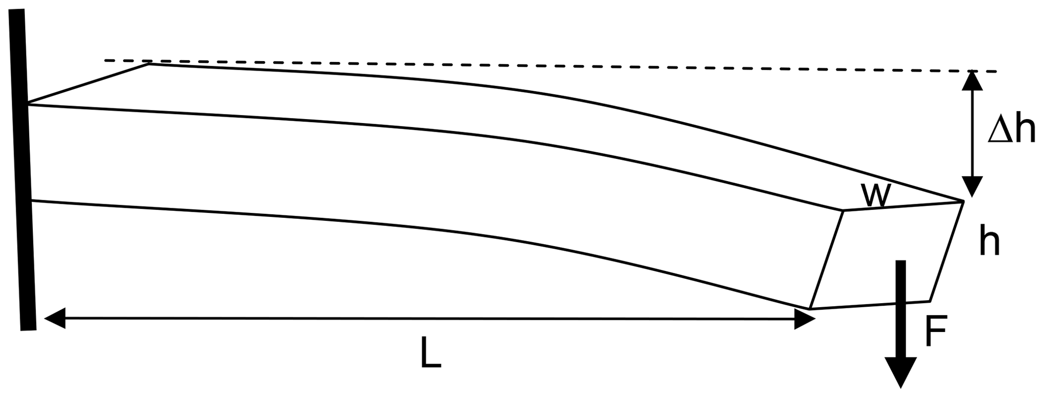
Figure 5Bending of a bar. When a given force F is applied as shown, the amount of bending Δh is proportional to L3, , and . Scaling all three quantities by the same factor leads to Δh (at a given force) being independent of L.
If, for simplicity, we assume the spectrograph to behave like a bar with length L, width w, and height h (see sketch in Fig. 5) on which an external force acts, then we can apply the famous case of bending a bar, which is described in most physics textbooks (see, for example, Meschede, 2015). When scaling the initial length L0 of the bar to some other length L by a factor and likewise w0 to and h0 to , we can calculate the scaling of Δh since
Since w and h are scaled proportional to L, we have
Thus the bar, in this case the spectrograph casing, will bend by the same absolute amount when subjected to a certain force. We can assume that the bending force actually scales with L as well because, for instance, thermal stress as well as external stress, for example, due to bending of the mounting base plate, is proportional to the dimension L. If we assume Hooke's law to hold, we can conclude that the deformation Δh of a spectrograph frame probably scales with . This, again, means that the performance of a scaled spectrograph will not change with scaling since the requirements for alignment of the optical elements also scale with L. For instance, in a scaled down spectrograph, the pixel size of the detector array will also shrink.
In conclusion, we can say that in first approximation, scaling of a spectrograph by changing all dimensions will not change its performance as far as it is determined by the geometry of the instrument, and therefore its mass will scale with L3 as assumed above.
Another point may be the thermal stability, which is a function of the thermal time constant of an object. The thermal time constant is given by the ratio of heat flow, being proportional to the surface of an object, and its heat capacity, which is (for a given material) proportional to the volume of the object. Thus the thermal time constant of a spectrometer should scale with .
Moreover, it can be assumed that a smaller instrument requires shorter and thus lighter wiring (although it amounts to only a small fraction of the total mass anyway).
3.3 How far can we shrink a spectrograph?
Obviously, we cannot shrink spectrographs indefinitely since then they will not function any more. In addition to possible mechanical constraints, the following phenomena (see also, for example, Avrutsky et al., 2006) limit the shrinking of spectrographs:
-
Light diffraction at the shrinking entrance slit will degrade the spectral resolution.
-
The grating will lose its resolving power.
-
Very small detector pixels are required.
In detail:
-
For a very long rectangular aperture (i.e. the entrance slit) with width wS (i.e. a slit with hS≫wS), the diffracted intensity is given by
Thus the first minimum is at x=π with . In order to use the slit image, at least the first diffraction order must hit the collimating mirror (or imaging grating); thus or . A more precise calculation actually yields wS being closer to (actually slightly smaller than) λ⋅F; thus for λ=320 nm and F=4, one obtains wS≈2 µm.
-
The resolving power of a grating with grating constant G (in grooves per millimetre) and width wG (in millimetres) is given by its total number of grooves, NG:
The smallest spectrographs typically used in (scattered sunlight) DOAS instruments are “miniature spectrographs”, like the Ocean Optics (Ocean Optics, 2020) USB2000 or Avantes AvaSpec-Mini (Avantes, 2020) instruments featuring f≈70 mm equipped with an entrance slit with wS=0.050 mm and hS=0.5 mm. The F number of the instruments is about 4, corresponding to an aperture solid angle .
The corresponding étendue will be m2 sr (0.00123 mm2 sr). The grating typically has 1800 grooves per millimetre, resulting in a total number of 36 000 grooves and a theoretical resolving power P=36 000. In practice, because of the relatively wide entrance slit, the spectral resolution is about 0.5 nm at 300 nm, corresponding to a resolving power Ppract≈600.
-
The detector arrays typically have a pixel pitch around 12 µm. If a spectrograph is to be scaled down, the pixel pitch must also be scaled (with the same linear scaling factor). Presently, detectors with pixel pitches around 1 µm are mass-produced and are used in many consumer products (smartphones, webcams, etc.). Although these sensors are primarily designed for visible light detection it has recently been shown that UV sensing is also possible with these cameras (Wilkes et al., 2017a, b).
In summary, even rather small, “miniature” spectrographs (like Ocean Optics USB2000 or AvaSpec-Mini) with focal lengths around f≈50–70 mm probably could be scaled down by . Thus, an array of 100 of such microspectrographs (+ telescope) could replace a conventional miniature spectrograph at about one-tenth of volume and weight. Of course for larger spectrographs such as those used in satellite instruments or active LP-DOAS, even higher scaling factors are in principle possible.
3.4 Spectrograph stray light
Here we have a quick look at the effect of spectrograph-system optimization on the stray light level. Stray light can have negative effects on the precision of spectroscopic trace gas measurements, as, for example, pointed out by Platt and Stutz (2008). Note that stray light can be comparatively high in spectrographs, filtering a relatively broad wavelength interval from a continuous spectrum as in typical DOAS applications. As also pointed out by Platt and Stutz (2008), a typical stray light level of as derived by illuminating the instrument with a monochromatic source (see, for example, Pierson and Goldstein, 1989) translates into stray light levels being closer to 10−2 than to 10−5.
Sources of stray light include light scattered by the optical elements (grating, mirrors, and the detector surface) of the instrument, reflection of unused diffraction orders off the spectrograph walls, reflection of unused portions of the spectrum from walls near the focal plane, and reflections from the detector surface (see, for example, Pierson and Goldstein, 1989). A further, potentially important source of stray light is due to incorrect illumination of the spectrograph: if the F number of the illumination exceeds that of the spectrograph, radiation will overfill the collimating mirror and hit interior walls of the instrument, from where it may be reflected to the detector.
In general, the amount of stray light is proportional to the ratio of the area of the scattering surfaces and the detector area; i.e. basically its amount scales with the inverse of the F number. Overall, it appears that the relative amount of stray light should not change when the spectrograph is scaled, such that its aspect ratio (and thus its F number) remains unchanged (i.e. according to case 1 in Table 1). Of course, running an array of spectrographs of identical design in parallel (case 4 in Table 1) should also not affect the relative amount of stray light.
3.5 Further considerations
It can be desirable to have a small or vanishing polarization sensitivity of spectrometers used for the analysis of sunlight reflected from Earth's surface or scattered in the atmosphere. In some satellite instruments, e.g. OMI and TROPOMI, “polarization scramblers” are used to reduce the polarization sensitivity of the spectrometer. There are many different designs of polarization scramblers (e.g. Lyot depolarizer or wedge depolarizer), which are based on plates consisting of birefringent material being placed in the optical path of the instrument; see, for example, Caron et al. (2012). These devices have in common that they are rather small plates consisting of two wedges (wedge angle around 1∘) made of birefringent material. These are placed in the optical path of the instrument, typically at a suitable position between the telescope entrance and the entrance slit. In the case of TROPOMI, two pairs of wedges (quartz and magnesium fluoride, respectively) are used, and their volume is around 1 cm3 (Babic et al., 2019).
Obviously, for very small spectrometers and telescopes, the depolarizer will also be very small (a fraction of 1 cm3), thus adding negligibly (<3 %) to the volume and weight of the instrument.
Another point which is particularly relevant for satellite applications is the use of direct solar reference spectra. The usual means of obtaining these spectra relies on directing sunlight via diffuser plates into the instrument. This approach, however, faces some technical difficulties due to the spectral structures introduced by the diffuser plates (see, for example, Richter and Wagner, 2001). Therefore, we recommend applying the “reference sector method” or related techniques, which are frequently used and do not rely on diffuser plates.
We also note that smaller instruments require shorter power (or data) connection wires; thermal ducts can also be shorter and thus lighter (see also Sect. 3.2). Similarly, radiation shielding (of e.g. detectors in satellite instruments from cosmic radiation) becomes much lighter for smaller instruments. Alternatively, one might want to keep the mass and thus the power lines and shielding constant and benefit from an enhanced light throughput. Moreover, using a large number of spectrometers in parallel has the potential advantage that the data from individual detectors, which were affected by cosmic radiation, can be sorted out and are not co-added during the evaluation procedure.
Finally, a spectrograph array design also reduces complexity since a much simpler optical design can be used for each pixel (or small number of pixels), which is just repeated many times (see, for example, Sect. 4.1). In fact, in most cases, a single (or a few) rather complex instrument(s) are replaced by a large number of comparatively simple instruments of identical design. There will likely be additional effort in cross-calibration, which, however may be offset by a simplified design.
3.6 How is the signal of a large number of spectrographs combined?
In principle, this is a straightforward task: if all individual spectrographs of an array (i.e. set of spectrographs with identical spectral ranges and viewing directions) were truly identical in spectral resolution and spectral registration (wavelength calibration and dispersion), then the detector output signal of corresponding pixels only had to be individually digitized and co-added. How well this prerequisite for simple co-adding is actually met depends on the manufacturing process and its precision for the individual (miniature) spectrographs. If the deviations of the individual spectrographs only amount to a fraction of a pixel, one might choose to still simply co-add the spectra and accept a certain degradation in spectral resolution.
If it should be found that the individual spectrographs have considerable individual deviations in spectral registration, a correction by shifting and stretching/compressing the individual spectra prior to co-adding might be necessary. These tasks require some effort in post-processing; however with the rapid advancement of electronics and information technology in recent decades, this should not be a major problem. For instance, advanced bus systems could be used to interconnect the individual spectrographs.
For satellite instruments (see Sect. 4.1, below), the idea is to basically have one (or a small number of) spectrometer(s) per viewing direction. In the case of a single spectrometer (with a 1-D detector) per viewing direction, there would be no change in the amount of data generated compared to an approach using a single spectrograph with a 2-D detector (as, for example, in the OMI or TROPOMI instruments). In designs where several spectrometers observe the same ground pixel (see Sect. 4.1), data could be co-added on board. Thus, again there would be no increase in data rate compared to a single spectrograph with a 2-D detector approach.
3.7 How are arrays of (micro)spectrographs manufactured?
Clearly, the widespread use of arrays of large numbers of (micro)spectrographs hinges on efficient manufacturing techniques for these instruments. Miniaturized spectrographs based on conventional spectrograph design are described by a number of authors, e.g. Avrutsky et al. (2006), Wilkes et al. (2017), and Danz et al. (2019). These authors also mention modern manufacturing techniques.
In particular, at present, technologies for mass production are available, like 3-D printing or automated machining of the frame. Also, the optical alignment of spectrographs can be automated; here replica optics could help. In addition, the required electronics and detectors have become very affordable during recent decades.
Furthermore, in the case of satellite instruments, space qualification and documentation of a large number of identical (and rather simple) spectrographs may mean less effort than that of a single or a few (relatively complicated) spectrographs.
3.8 Unconventional spectrograph designs
A number of ideas for unconventional spectrograph designs were reported. For instance, how to enhance the light throughput of imaging spectrographs (for the visible and near-IR spectral range) is presented by Chrisp et al. (2020). Park and Choi (2013) suggested Fresnel optics to miniaturize spectrographs. Furthermore, a completely new principle for spectrograph design was proposed, for example, by Grundmann (2019a, b); it relies on using a special type of diode array as the only element of the instrument. The pixels of the diode array are manufactured in such a way that the bandgap of the semiconductor increases with the pixel number (this is achieved using a binary or ternary semiconductor with a composition varying with the pixel position). The light enters along the long axis of the detector array (which acts as a waveguide) at pixel 1, which has the smallest bandgap and therefore absorbs the longest wavelength radiation while transmitting radiation with shorter wavelength. Pixel 2 has a slightly wider bandgap absorbing radiation with slightly (by Δλ) shorter wavelength and so forth. The resolution of the device is approximately equivalent to Δλ. In a practical device, a spectral resolution of 0.01 eV at 3.5 eV (corresponding to about Δλ≈1 nm at ≈355 nm) was reached.
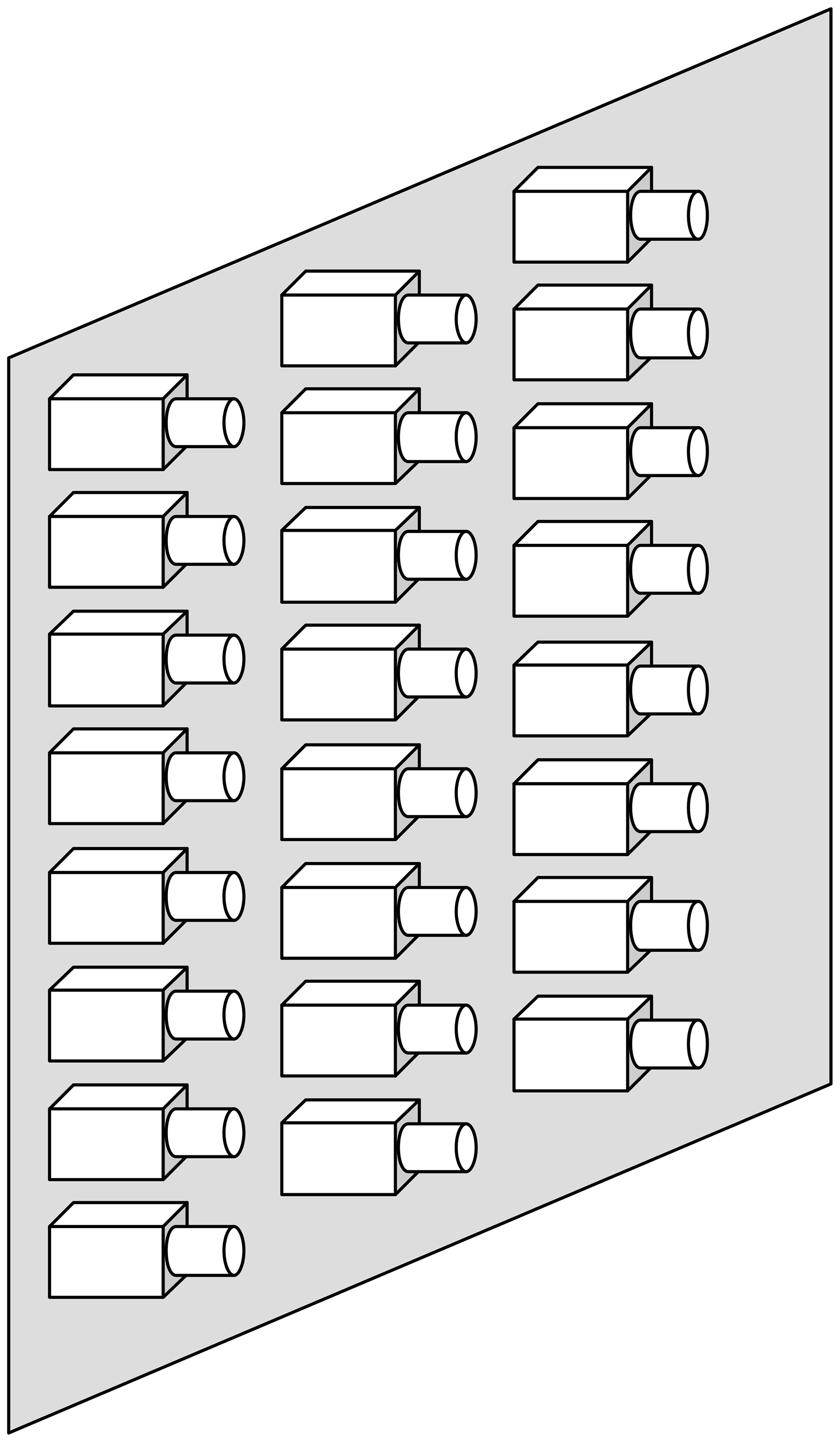
Judging from the above considerations, in most applications, replacement of existing spectrographs by an array of scaled-down microspectrographs of identical design (see Fig. 6) would result in considerable (up to 2 to 3 orders of magnitude) reduction in volume and weight. As mentioned above, even if miniature spectrographs are taken as a basis for comparison, an order of magnitude reduction appears possible.
4.1 Satellite applications
There are a number of satellite instruments in orbit (e.g. GOME, GOME-2A, B, C, SCIAMACHY, ODIN, OMI, TROPOMI, OMPS NM, GEMS (geostationary), EMI) which are based on small UV–visible–near-IR spectrographs (typical focal length around 200 mm) coupled to small telescopes (typical diameter 1 cm). The typical telescope field-of-view angle (for 1 ground pixel) is around 0.25 to 1∘.
Usually per wavelength range, one spectrograph is used. The total number of spectrographs is two (OMI; Levelt et al., 2006), four (TROPOMI; Veefkind et al., 2012; Dobber et al., 2006), four (GOME and GOME-2; Burrows, 1999), and eight (SCIAMACHY; Burrows and Chance, 1991; Goede et al., 1991; Burrows et al., 1995; Bovensmann et al., 1999).
The scanning (i.e. cross-track spatial resolution) is either achieved by a mechanical scanner or by imaging spectrographs (2-D spectrographs, where one dimension is devoted to wavelength, the second to space); see, for example, Levelt et al. (2006) or Veefkind et al. (2012). In particular, these imaging instruments are very sophisticated designs featuring extreme properties like very large cross-track fields of view combined with extremely small along-track aperture angles. These truly remarkable features come at a price: in some cases aspherical (or even free-form) optics have to be used, and only rather large F numbers are possible.
In order to reduce the weight and volume of instruments of this type, the single spectrograph (per wavelength range) could be replaced by an array of scaled down spectrographs, each observing 1 or a few ground pixels. Each spectrograph would have its own telescope; thus cross-track resolution could be achieved by aligning the field of view of the individual spectrographs accordingly, as sketched in Fig. 7a. Thereby the advantages of avoiding scanners by using the pushbroom principle are combined with a rather simple design (of the individual telescopes).
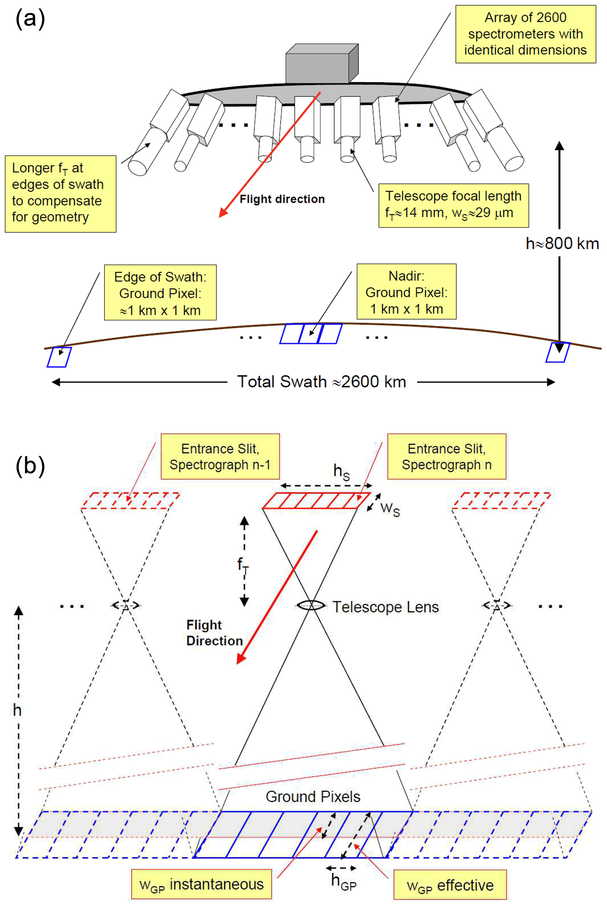
Figure 7(a) Possible arrangement of an array of spectrograph + telescope combinations for satellite application (this example depicts the “scaled 2” arrangement; see Table 2). In principle, there is one spectrograph + telescope for a viewing direction (i.e. ground pixel; see Table 2). (In the case of the “scaled 2” arrangement, two spectrographs observe the same ground pixel to improve the ratio.) Longer focal lengths fT of the telescope observing ground pixels near the edge of the swath could be chosen to compensate for their larger size. For simplicity, a linear arrangement of the spectrographs along a line is shown; in practice an arrangement in a 2-D array would of course be much more compact. (b) Relationship between the spectrograph entrance slit, instantaneous field of view, and the pixel dimensions. This example depicts a section of the “scaled 1” arrangement, where each spectrograph observes 6 ground pixels; see Table 2.
In fact, there could be one or several spectrographs per viewing direction and wavelength interval. This approach would have no more drawbacks, for instance, with respect to “destriping” measures, than existing whisk-broom designs (like OMI or TROPOMI). The cause(s) for the “striping phenomenon” (slight changes in the derived slant column density (SCD) values across the swath) are not fully understood, but it is probably due to somewhat different instrument functions for each viewing direction. On the other hand, such a spectrograph per viewing direction (SPVD) approach could have great advantages besides the obvious possibility of achieving better light throughput and thus SNR:
-
A much simpler spectrometer design. Here a conventional Czerny–Turner design or imaging grating design is assumed. Additional light throughput could be gained by the measures described in Sect. 2.3. Obviously the telescope has to be designed in such a way that the projection of the ground pixel matches the spectrograph entrance slit size (see Fig. 7b).
-
A much simpler telescope design. Only a small telescope field of view is required.
-
An adaptive field of view for the edges of the swath (for a daily coverage by a LEO instrument, a ≈2600 km swath is needed). This is in order to reduce the variation in ground pixel size across the swath. At 800 km satellite altitude, the pixels at the edge of the swath are roughly twice as long (along-track extension) and 4 times as wide (cross-track extension) than in the centre of the swath, i.e. in a satellite nadir direction (see Fig. 7a).
-
More redundancy in the design. The failure of an individual spectrograph would not be catastrophic.
Regarding the ground pixel size, there are three reasons why the ground pixels are larger towards the edges of the swath (assumed here to be 2600 km at a satellite altitude of 800 km):
-
The pixels at the edge of the swath are further away from the instrument. This effect enlarges the pixels by a factor of 1.91 in the cross-track as well as in the along-track direction (area is thus enlarged by a factor of 3.64).
-
The pixels at the edge of the swath are seen under a larger angle (≈58.4∘); thus their cross-track extension (but not the along-track extension) is further enlarged by another factor of 1.91, enhancing its cross-track extension to 3.64 over the nadir case (area increases by a factor of 6.94).
-
The larger angle at which the pixels at the edge of the swath are seen is further enlarged due to the curvature of Earth (enlarging the viewing angle at the edge of the swath by 11.5∘), bringing the total angle to 69.9∘. Thus the cross-track extension of the ground pixel is extended by a factor of 5.56 instead of 3.64 for the flat Earth case (or an additional factor of 1.52). Ultimately the ground pixel area is larger than in nadir by a factor of 10.6.
This latter effect (curvature of Earth) has the smallest influence on the ground pixel size at the edge of the swath. Thus a “flat Earth” approximation could be considered for the sake of simplicity.
In the following, we give two examples of possible satellite instruments based on arrays of microspectrographs. The hypothetical instrument designs are compared to the TROPOMI instrument, for simplicity, we only simulated the UV–Vis section of TROPOMI, but other wavelength ranges could be readily added. Relevant instrument parameters are summarized in Table 2:
-
One instrument (“Scaled 1”) has data similar to the TROPOMI UV–Vis section (Dobber et al., 2006; Veefkind et al., 2012; Babic et al., 2019), where the individual spectrographs are scaled down to approximately . For compensation, 100 spectrographs, each observing 6 ground pixels, would be run in parallel. The total étendue (≈0.065 mm2 sr) of all spectrographs (variant A) would be somewhat smaller than the total étendue of the TROPOMI instrument (≈0.103 mm2 sr). Therefore, we added another variant (B) of the instrument encompassing 200 spectrometer + telescope combinations (data given in square brackets in Table 2), arranged in two identical sets of 100 spectrometer + telescope combinations. In either case, each spectrograph would have its own (now very small; see Table 2) telescope. In the case of using 200 spectrographs (variant B), each set of 6 ground pixels would be observed by two spectrographs, thus doubling the étendue (to ≈0.13 mm2 sr) and the signal, which would then exceed that of TROPOMI (alternatively, each spectrograph+telescope could observe only 3 ground pixels). Note that the total mass of the “scaled 1” instrument (not just one spectrometer) as given in the last line of Table 2 is about of that of the TROPOMI instrument. This case also illustrates the design flexibility given by the spectrograph array approach.
-
One instrument (“Scaled 2”) is capable of scanning at a ground pixel size of 1 km×1 km. Here a total of 2600 spectrograph + telescope combinations would be employed, each observing 8 ground pixels, while eight spectrographs observe the same set of 8 ground pixels. This arrangement would observe ground pixels about 25 times smaller than TROPOMI at a comparable SNR and weight.
Data for TROPOMI are taken from Veefkind et al. (2012), Kleipool et al. (2018), Babic et al. (2019), and Dobber et al. (2006). As can be seen from Table 2, scaling down the spectrograph size can provide much smaller and lighter instruments (e.g. scaled 1 will be roughly of the weight compared to the TROPOMI instrument) while featuring similar signal-to-noise levels. As an option, the scaled instruments could at the same time feature constant ground pixels size at the edges of the swath range, while the OMI and TROPOMI instruments ground pixels are larger than the nadir pixels by factors of approximately 1.9 (along track) and 5.6 (cross track); see, for instance, OMI-DUG-5.0 (2012). In Table 2, we apply a factor of up to 3.25 enhancement of magnification (i.e. enhancement of telescope focal length) in order to keep the pixel area constant across the entire swath.
Table 2Typical data of TROPOMI-Type and scaled satellite instruments working in the UV for a spectral resolution of ca. 0.5 nm. “Scaled 1” refers to an instrument approximately matching the data of the TROPOMI UV–Vis part, employing 100 (variant A) or 200 (variant B) spectrographs + telescopes; the latter values are given in square brackets. “Scaled 2” refers to an instrument encompassing 2600 spectrographs + telescopes with 1 km by 1 km ground pixels.

a See Dobber et al. (2006), Veefkind et al. (2012), Kleipool et al. (2018), and Babic et al. (2019). b Not applicable in this context due to intermediate imaging. c Calculated from telescope F number and entrance area as given by Dobber et al. (2006) and Babic et al. (2019). d A factor of up to 3.25 magnification enhancement (i.e. increase of fT) is applied in order to keep the pixel area constant across the entire swath. However, for 60 % of the pixels (centre 1600 km of swath), the necessary extension of fT is <2. e In the case of TROPOMI, only the volume of the UV–Vis section.
The instrument (scaled 2) with 1 km by 1 km ground pixels throughout the swath with much (about 16.5) higher total étendue and comparable étendue per pixel (see Table 2) would provide a comparable signal-to-noise ratio as TROPOMI despite the 25 times smaller ground pixel area and could also feature constant ground pixel dimensions across the entire swath. For comparison, in order to achieve the same total étendue by just scaling up the instrument dimensions (e.g. from a TROPOMI-type instrument with M0≈100 kg) according to Eq. (5), a total instrument mass of or around 7 t would be required.
Obviously these are just examples to illustrate the potential of the new approach. Further spectrograph downscaling (for instance, to f=10 mm) would be possible. In addition, other combinations of spectrograph–pixel arrangements as well as the inclusion of further measures for improved light throughput (immersed gratings, imaging optics; see Sect. 2.3) are possible and must be explored.
4.2 MAX-DOAS applications
MAX-DOAS spectrographs are typically equipped with miniature spectrographs (e.g. Ocean Optics, Avantes). Here, similar considerations apply as in the case of satellite instruments. For instance the typically used single spectrograph could be replaced by an array of scaled down spectrograph + telescope combinations as sketched in Fig. 6. In the simplest case, all spectrographs could point in the same direction, and the whole assembly would be tilted to measure at different elevation angles. Alternatively, the spectrograph + telescopes could point at different elevations, thus analysing the radiation at the chosen set of elevation angles simultaneously (see, for example, Leigh et al., 2007). While the latter approach would have the advantage that all elevations are observed truly simultaneously (as opposed to sequentially in the former approach), a problem could arise from slight differences in the instrument function of the individual spectrographs. Unlike the satellite case, there would be no natural way where all spectrographs see the same spectrum (e.g. by observing in the zenith direction).
In either case, one could argue that weight and volume of the spectrograph only constitute a small fraction of that of the entire MAX-DOAS instrument; however, the size of the instrument still scales with the spectrograph dimensions. Alternatively, the scaling could be used to enhance the étendue of the instrument and thus allow for proportionally faster measurements.
4.3 Imaging DOAS applications
Another use of large arrays of spectrographs (+ telescopes) could be imaging applications where the usual need to make a compromise between spectral, spatial, and temporal resolution (see, for example, Platt et al., 2015) is removed or at least relaxed. For instance, an array of spectrographs (similar to the approach described by Danz et al., 2019) could be arranged with a spectrograph per image pixel in a compound eye (as found in insects) fashion.
4.4 Other applications
Arrays of (miniature) spectrographs could also be applied in active long-path DOAS (LP-DOAS) instruments. In this case, a single, large telescope could be replaced by an array of small telescopes. As discussed above, the F number of these small telescopes would be about the same as in present instruments. If the total area covered by the telescope mirrors were the same, then there would be the same light throughput as in conventional active LP-DOAS designs. In this case, not only could the volume and weight of the spectrographs be reduced, but also the length of the telescope. This is because the F number of each small telescope remains unchanged (compared to traditional designs), while the diameter of the mirror (or lens) – and thus its focal length f – is scaled down.
5.1 Summary of design options
Arrays of individual (largely identical) spectrographs could help to solve a number of design challenges for both satellite instruments and other applications.
-
Spectrograph arrays allow the Étendue and thus SNR to be improved independently from the spatial resolution.
-
Due to the scaling properties of volume and mass, replacing large spectrographs with an array of smaller (identical) spectrographs can reduce the volume and mass of a spectrograph system considerably.
-
Spatial information (e.g. in satellite or MAX-DOAS applications) could be obtained in a much simpler fashion than in present-day arrangements.
-
Two-dimensional imaging detectors based on arrays of miniature spectrographs appear feasible.
Clearly, the individual spectrographs might have somewhat different responses, but this is not different to the present situation where the individual lines of pixels (corresponding to the spatial resolution) have somewhat different responses. The pointing accuracy is a matter of the platform. Minimizing possible changes between the relative pointing of the individual spectrographs is a design issue, which will not be addressed here.
5.2 Conclusion
We conclude that arrays of massively parallel spectrographs could solve the problem of achieving high light throughput with compact and lightweight instruments.
In particular, a reduction of the instrument volume and mass by 1 or 2 orders of magnitude at unchanged light throughput appears possible. This might be interesting for a number of particular design goals for satellite instruments:
-
Miniature satellites (e.g. CubeSats) could be equipped with spectrographs for Earth observation featuring sensitivity and spatial resolution comparable to present state-of-the-art instruments (like GOME-2, OMI, or even TROPOMI).
-
Instruments for future missions could reduce the area of the ground pixels by 1 or 2 orders of magnitude without increasing the mass and size of the spectrograph.
-
If a higher mass of the instrument were allowed, the spectrograph array approach would allow the area of the ground pixels to be reduced even further. Thus, an instrument (see above) with 1 km2 ground pixel size could feature a comparable volume and mass to a present state-of-the-art (e.g. the TROPOMI) spectrograph.
Also, the scaling of instruments using the spectrograph array approach will be of great interest to other DOAS applications as well:
-
aircraft (manned or unmanned) instruments, which have similar requirements to satellite instruments;
-
MAX-DOAS instruments;
-
instruments for monitoring volcanoes (as, for example, used in NOVAC);
-
imaging DOAS applications;
-
active LP-DOAS instruments there, in particular the telescope size, can be reduced by employing the spectrograph + telescope-array approach.
We acknowledge that there might be some technical hurdles like mass production of spectrographs with as similar instrument functions and other characteristics as possible or the readout of many spectrographs in parallel. Also, potential problems associated with aligning and testing many spectrographs (+ telescopes) have to be solved.
However, instrument properties, like radiometric accuracy and stability, initially and – in the case of 20 satellite instruments – over the entire mission, are rather questions of the particular instrument design. They have no direct connection to the question of how many individual spectrographs are used. Nevertheless, we are convinced that massively parallel miniature spectrographs are an attractive approach for future instruments.
The change of the spectrometer, with initial étendue E0, initial focal length f0, and optics diameter D0 to Γ1f0 with constant optics diameter D0, can be thought of as a two-step process:
-
Scale the entire spectrometer with a preserved aspect ratio (according to case 1 in Table 1) by a linear factor Γ1 (for example ) → E will be reduced to (Γ1)2 (i.e. to ), while the mass will change from M0 to M0⋅(Γ1)3 (i.e. to ). Note that the slit dimensions are also scaled by Γ1.
-
Then increase D by factor (according to case 2a in Table 1) → in this step E and mass will increase by factor .
In total, E would be unchanged, and mass will be scaled to M0⋅Γ1 (i.e. to ).
-
Since we assumed that in case 2b (see Table 1) the slit width is scaled but not the slit height, we have to change the slit height from Γ1⋅h0 to its original value h0.
→ The final E will be (i.e. E=2E0); thus , as given in Eq. (9).
No data sets were used in this article.
All the authors (UP, TW, JK, TL) contributed to the development of the ideas presented in the manuscript, and all authors worked on aspects of the text. UP wrote most of the manuscript.
Ulrich Platt and Thomas Wagner are members of the editorial board of AMT. Thomas Leisner and Jonas Kuhn declare that they have no conflict of interest.
Publisher's note: Copernicus Publications remains neutral with regard to jurisdictional claims in published maps and institutional affiliations.
The authors would like to thank the German Science Foundation (DFG) for partial funding through project PL 193/23-1-3016731. We are also thankful to the Max Planck Society for covering the article processing charges for this open-access publication.
Part of the work was funded by the German Science Foundation (DFG) through project PL 193/23-1-3016731.
The article processing charges for this open-access publication were covered by the Max Planck Society.
This paper was edited by Mark Weber and reviewed by two anonymous referees.
Avantes: AvaSpec-Mini Data sheet, Avantes BV, Apeldoorn, the Netherlands, available at: https://www.avantes.com, last access: 17 November 2020.
Avrutsky, I., Chaganti, K., Salakhutdinov, I., and Auner, G.: Concept of a miniature optical spectrometer using integrated optical and micro-optical components, Appl. Optics, 45, 7811–7817, 2006.
Babic, L., Braak, R., Dierssen, W., Kissi-Ameyaw, J., Kleipool, Q., Leloux, J., Loots, E., Ludewig, A., Rozemeijer, N., Smeets, J., and Vacanti, G.: Algorithm theoretical basis document for the TROPOMI L01b data processor, The Royal Netherlands Meteorological Institute KNMI, Document no. S5P-KNMI-L01B-0009-SD, Issue 9.0.0, 19 July 2019, https://sentinels.copernicus.eu/documents/247904/2476257/Sentinel-5P-TROPOMI-Level-1B-ATBD (last access: 15 October 2021), 2019.
Barducci, A., Guzzi. D., Lastri, C., Marcoionni, P., Nardino, V., and Pippi. I.: Fourier Transform Spectrometry: the SNR disadvantage of the multiplex architecture, in Imaging and Applied Optics, OSA Technical Digest (CD), paper FWA5, Optical Society of America, Washington, DC, USA, https://doi.org/10.1364/FTS.2011.FWA5, 2011.
Blumenthaler, M., Gröbner, J., Huber, M., and Ambach, W.: Measuring spectral and spatial variations of UVA and UVB sky radiance, Geophys. Res. Lett., 23, 547–550, 1996.
Bovensmann, H., Burrows, J. P., Buchwitz, M., Frerick, J., Rozanov, V. V., Chance, K. V., and Goede, A. P. H.: SCIAMACHY: Mission objectives and measurement modes, J. Atmos. Sci., 56, 127–150, 1999.
Burrows, J. P. and Chance, K. V.: Scanning imaging absorption spectrometer for atmospheric chartography, Proc. SPIE, 1490, 146–155, 1991.
Burrows, J. P., Hölzle, E., Goede, A. P. H., Visser, H., and Fricke, W.: SCIAMACHY – Scanning Imaging Absorption Spectrometer for Atmospheric Chartography, Acta Astronaut., 35, 445–451, 1995.
Burrows, J. P., Weber, M., Buchwitz, M., Rozanov, V., Ladstätter-Weißenmayer, A., Richter, A., DeBeek, R., Hoogen, R., Bramstedt, K., Eichmann, K.-U., Eisinger, M., and Perner, D.: The Global Ozone Monitoring Experiment (GOME): Mission Concept and First Scientific Results, J. Atmos. Sci., 56, 151–171, 1999
Caron, J., Bézy, J.-L., Courrèges-Lacoste, G. B., Sierk, B., Meynart, R., Richert, M., and Loiseaux, D.: Polarization scramblers in Earth observing spectrometers: lessons learned from Sentinel-4 and 5 phases A/B1, in: International Conference on Space Optics, 9–12 October 2012, Ajaccio Corse, 2012.
Chrisp, M. P., Lockwood, R. B., Smith, M. A., Balonek, G., Holtsberg, C., Thome, K. J., Murray, K. E., and Ghuman, P.: Development of a compact imaging spectrometer form for the solar reflective spectral region, Appl. Optics, 59, 10007–10014, https://doi.org/10.1364/AO.405303, 2020.
Czerny, M. and Turner, A. F.: Über den Astigmatismus bei Spiegelspektrometern, Z. Phys., 61, 792–797, https://doi.org/10.1007/BF01340206, 1930.
Danz, N., Höfer, B., Förster, E., Flügel-Paul, T., Harzendorf, T., Dannberg, P., Leitel, R., Kleinle, S., and Brunner, R.: Miniature integrated micro-spectrometer array for snap shot multispectral sensing, Opt. Express, 27, 5719–5728, https://doi.org/10.1364/OE.27.005719, 2019.
Dobber, M. R., Dirksen, R. J., Levelt, P. F., van den Oord, G. H. J., Voors, R. H. M., Kleipool, Q., Jaross, G., Kowalewski, M., Hilsenrath, E., Leppelmeier, G. W., de Vries, J., Dierssen, W., and Rozemeijer, N. C.: Ozone Monitoring Instrument Calibration, IEEE T. Geosci. Remote, 44, 1209–1238, 2006.
Fastie, W. G.: Image Forming Properties of the Ebert Monochromator, J. Opt. Soc. Am., 42, 647–651, 1952.
Fellgett, P. B.: On the Ultimate Sensitivity and Practical Performance of Radiation Detectors, J. Opt. Soc. Am., 39, 970–976, https://doi.org/10.1364/JOSA.39.000970, 1949.
Ferlemann, F., Bauer, N., Fitzenberger, R., Harder, H., Osterkamp, H., Perner, D., Platt, U., Schneider, M., Vradelis, P., and Pfeilsticker, K.: Differential Optical Absorption Spectroscopy Instrument for stratospheric balloon-borne trace gas studies, Appl. Optics, 39, 2377–2386, 2000.
Galle, B., Johansson, M., Rivera, C., Zhang, Y., Kihlman, M., Kern, C., Lehmann, T., Platt, U., Arellano, S., and Hidalgo, S.: Network for Observation of Volcanic and Atmospheric Change (NOVAC) – A global network for volcanic gas monitoring: Network layout and instrument description, J. Geophys. Res., 115, D05304, https://doi.org/10.1029/2009JD011823, 2010.
General, S., Pöhler, D., Sihler, H., Bobrowski, N., Frieß, U., Zielcke, J., Horbanski, M., Shepson, P. B., Stirm, B. H., Simpson, W. R., Weber, K., Fischer, C., and Platt, U.: The Heidelberg Airborne Imaging DOAS Instrument (HAIDI) – a novel imaging DOAS device for 2-D and 3-D imaging of trace gases and aerosols, Atmos. Meas. Tech., 7, 3459–3485, https://doi.org/10.5194/amt-7-3459-2014, 2014.
Goede, A. P. H., Aarts, H. J. M., van Baren, C., Burrows, J. P., Chance, K. V., Hoekstra, R., Hölzle, E., Pitz, W., Schneider, W., Smorenburg, C. Visser, H., and de Vries, J.: Sciamachy instrument design, Adv. Space Res., 11, 243–246, https://doi.org/10.1016/0273-1177(91)90427-L, 1991.
Grundmann, M.: Monolithic Waveguide-Based Linear Photodetector Array for Use as Ultracompact Spectrometer, IEEE T. Electron Dev., 66, 470–477, 2019a.
Grundmann, M.: Modelling of a Waveguide-Based UV-Vis-IR Spectrometer Based on a Lateral (In,Ga)N Alloy Gradient, Phys. Status Solidi A, 216–221, 1900170, https://doi.org/10.1002/pssa.1900170, 2019b.
Haldane, J. B. S.: On Being the Right Size, in: Possible Worlds and other essays, Chatto and Windus, London, 1927.
Hönninger, G. and Platt, U.: The Role of BrO and its Vertical Distribution during Surface Ozone Depletion at Alert, Atmos. Environ., 36, 2481–2489, 2002.
Kleipool, Q., Ludewig, A., Babić, L., Bartstra, R., Braak, R., Dierssen, W., Dewitte, P.-J., Kenter, P., Landzaat, R., Leloux, J., Loots, E., Meijering, P., van der Plas, E., Rozemeijer, N., Schepers, D., Schiavini, D., Smeets, J., Vacanti, G., Vonk, F., and Veefkind, P.: Pre-launch calibration results of the TROPOMI payload on-board the Sentinel-5 Precursor satellite, Atmos. Meas. Tech., 11, 6439–6479, https://doi.org/10.5194/amt-11-6439-2018, 2018.
Kuhn, J., Bobrowski, N., Wagner, T., and Platt, U.: Mobile and high spectral resolution Fabry Pérot interferometer spectrographs for atmospheric remote sensing, Atmos. Meas. Tech. Discuss. [preprint], https://doi.org/10.5194/amt-2021-133, in review, 2021.
Larsson, T. and Neuhaus, H.: The Immersion Grating: Spectroscopic Advantages and Resemblance to the Echelon Grating, Z. Naturforsch., 23a, 2130–2132, 1968.
Leigh, R. J., Corlett, G. K., Frieß, U., and Monks, P. S.: Spatially resolved measurements of nitrogen dioxide in an urban environment using concurrent multi-axis differential optical absorption spectroscopy, Atmos. Chem. Phys., 7, 4751–4762, https://doi.org/10.5194/acp-7-4751-2007, 2007.
Levelt, P. F., van den Oord, G. H. J., Dobber, M. R., Mälkki, A., Visser, H., de Vries, J., Stammes, P., Lundell, J. O. V., and Saari, H.: The Ozone Monitoring Instrument, IEEE T. Geosci. Remote, 44, 1093–1101, https://doi.org/10.1109/TGRS.2006.872333, 2006.
Meschede, Dieter: Gerthsen Physik, Springer-Verlag, Berlin, Heidelberg, ISBN 978-3-662-45976-8, 2015.
Munro, R., Lang, R., Klaes, D., Poli, G., Retscher, C., Lindstrot, R., Huckle, R., Lacan, A., Grzegorski, M., Holdak, A., Kokhanovsky, A., Livschitz, J., and Eisinger, M.: The GOME-2 instrument on the Metop series of satellites: instrument design, calibration, and level 1 data processing – an overview, Atmos. Meas. Tech., 9, 1279–1301, https://doi.org/10.5194/amt-9-1279-2016, 2016.
Ocean Optics: USB2000+ Data sheet, Ocean Optics (now: Ocean Insight), Dunedin, Florida, 34698, USA, https://www.oceaninsight.com/ (last access: 17 November 2020), 2020.
OMI-DUG-5.0: Produced by OMI Team, Ozone Monitoring Instrument (OMI) Data User's Guide, available at: https://docserver.gesdisc.eosdis.nasa.gov/repository/Mission/OMI/3.3_ScienceDataProductDocumentation/3.3.2_ProductRequirements_Designs/README.OMI_DUG.pdf (last access: 15 October 2021), 2012.
Park, Y. and Choi, S. H.: Miniaturization of optical spectroscopes into Fresnel microspectrometers, J. Nanophotonics, 7, 077599, https://doi.org/10.1117/1.JNP.7.077599, 2013.
Pierson, A. and Goldstein, J.: Stray light in spectrometers: causes and cures, Lasers Optron., 8, 67–74, 1989.
Platt, U. and Stutz, J.: Differential Optical Absorption spectroscopy, Principles and Applications, XV, Springer, Heidelberg, 597 pp., 272 illus., 29 in color (Physics of Earth and Space Environments), ISBN 978-3-540-21193-8, 2008.
Platt, U., Lübcke, P., Kuhn, J., Bobrowski, N., Prata, F., Burton, M. R., and Kern, C.: Quantitative Imaging of Volcanic Plumes – Results, Future Needs, and Future Trends (JVGR, SI on Plume Imaging), J. Volcanol. Geoth. Res., 300, 7–21, https://doi.org/10.1016/j.jvolgeores.2014.10.006, 2015.
Richter, A. and Wagner, T.: Diffuser plate spectral structures and their influence on GOME slant columns, Technical Note to ESA, January 2001, available at: http://joseba.mpch-mainz.mpg.de/pdf_dateien/diffuser_gome.pdf (last access: 15 October 2021), 2001.
Schilling, S.: Lens Array captures dim objects missed by giant telescopes, Science, 371, 1301, https://doi.org/10.1126/science.371.6536.1301, 2021.
Sinreich, R., Frieß, U., Wagner, T., and Platt, U.: Multi axis differential optical absorption spectroscopy (MAXDOAS) of gas and aerosol distributions, Faraday Discuss., 130, 153–164, https://doi.org/10.1039/B419274P, 2005.
van Amerongen, A. H., Visser, H., Vink, R. J. P., Coppens, T., and Hoogeveen, R. W. M.: Development of immersed diffraction grating for the TROPOMI-SWIR Spectrometer, Proc. SPIE, 7826, 78261D-1, https://doi.org/10.1117/12.869018, 2010.
Veefkind, J. P., Aben, I., McMullan, K., Förster, H., de Vries, J., Otter, G., Claas, J., Eskes, H. J., de Haan, J. F., Kleipool, Q., van Weele, M., Hasekamp, O., Hoogeveen, R., Landgraf, J., Snel, R., Tol, P., Ingmann, P., Voors, R., Kruizinga, B., Vink, R., Visser, H., and Levelt, P. F.: TROPOMI on the ESA Sentinel-5 Precursor: A GMES mission for global observations of the atmospheric composition for climate, air quality and ozone layer applications, Remote Sens. Environ., 120, 70–83, 2012.
Wilkes, T. C., McGonigle, A. J. R., Willmott, T. D., Pering, T. D., and Cook, J. M.: Low-cost 3D printed 1 nm resolution smartphone sensor-based spectrometer: Instrument design and application in ultraviolet spectroscopy, Opt. Lett., 42, 4323–4326, 2017.