Deriving column-integrated thermospheric temperature with the N₂ Lyman–Birge–Hopfield (2,0) band

This paper presents a new technique to derive thermospheric temperature from space-based disk observations of far ultraviolet airglow. The technique, guided by findings from principal component analysis of synthetic daytime Lyman–Birge–Hopfield (LBH) disk emissions, uses a ratio of the emissions in two spectral channels that together span the LBH (2,0) band to determine the change in band shape with respect to a change in the rotational temperature of N₂. The two-channel-ratio approach limits representativeness and measurement error by only requiring measurement of the relative magnitudes between two spectral channels and not radiometrically calibrated intensities, simplifying the forward model from a full radiative transfer model to a vibrational–rotational band model. It is shown that the derived temperature should be interpreted as a column-integrated property as opposed to a temperature at a specified altitude without utilization of a priori information of the thermospheric temperature profile. The two-channel-ratio approach is demonstrated using NASA GOLD Level 1C disk emission data for the period of 2–8 November 2018 during which a moderate geomagnetic storm has occurred. Due to the lack of independent thermospheric temperature observations, the efficacy of the approach is validated through comparisons of the column-integrated temperature derived from GOLD Level 1C data with the GOLD Level 2 temperature product as well as temperatures from first principle and empirical models. The storm-time thermospheric response manifested in the column-integrated temperature is also shown to corroborate well with hemispherically integrated Joule heating rates, ESA SWARM mass density at 460 km, and GOLD Level 2 column $\mathrm{O}/{\mathrm{N}}_{\mathrm{2}}$ ratio.

1 Introduction

Remote sensing of Earth's far ultraviolet (FUV) airglow from space provides important insights into the energetics, dynamics, and composition of the upper atmosphere (Meier, 1991; Paxton et al., 2017). The N₂ Lyman–Birge–Hopfield (LBH) bands (∼127–280 nm) are prominent daytime FUV airglow features that emanate from the lower to middle thermosphere (∼120–200 km). Currently operating instruments measuring the LBH bands include the Thermosphere-Ionosphere-Mesosphere Energetics and Dynamics (TIMED) satellite's Global Ultraviolet Imager (GUVI) launched in 2001 (Christensen et al., 2003), the Defense Meteorological Satellite Program's (DMSP) Special Sensor Ultraviolet Spectrographic Imager (SSUSI) launched in 2003 (Paxton et al., 2002), the Global-scale Observations of the Limb and Disk (GOLD) launched in 2018 (McClintock et al., 2020a), and the Ionospheric Connection Explorer's Far UltraViolet imaging spectrograph (FUV) launched in 2019 (Mende et al., 2017).

The utility of the LBH bands for probing thermospheric temperature was demonstrated by Aksnes et al. (2006) with limb observations by the Advanced Research and Global Observation Satellite's (ARGOS) High-resolution Ionospheric and Thermospheric Spectrograph (HITS) instrument. Eastes et al. (2008) subsequently showed that disk observations of LBH bands could be used for global monitoring of thermospheric temperature. These authors fit LBH laboratory spectra to observed emissions using an optimal estimation routine with varying parameters such as the N₂ rotational temperature, population rates of each vibrational band, the NI 149.3 nm line emission intensity, O₂ photoabsorption, and background emission rates. GOLD is the first mission to provide a Level 2 data product of thermospheric temperature (T_DISK) using LBH disk emissions between ∼132–162 nm with a similar retrieval implementation (Eastes et al., 2017). Thermospheric temperatures have also been derived from TIMED GUVI observations (Zhang et al., 2019) using an intensity ratio between the (0,0) band and (1,0) band that the authors found to be quasi-linearly dependent on the N₂ rotational temperature. The authors attributed the temperatures to the altitude at the peak of the LBH contribution function (∼155 km) based on radiative transfer calculations.

This paper presents a new technique to derive thermospheric temperature from spectrographic measurements of FUV airglow. The technique, unlike in past work, uses the ratio of two spectral channels that span a single LBH band to determine the change in band shape with respect to a change in the rotational temperature of N₂. Section 2 provides background and exploration of the LBH temperature signal with principal component analysis (PCA) to motivate the new technique. Section 3 details the implementation and provides a discussion on the error sources and a rationale behind our interpretation of the derived temperature as a column-integrated property that we refer to as column-integrated thermospheric temperature, T_ci. Section 4 presents the demonstrative results of applying the technique to GOLD Level 1C radiance data for the period of 2–8 November 2018, during which a moderate geomagnetic storm event occurred. The derived thermospheric temperatures are compared to the GOLD Level 2 version 3 T_DISK data product over the same period. Due to the lack of independent remotely sensed or in situ temperature measurements in the lower to middle thermosphere, the derived column-integrated temperatures are also compared to (1) synthetically generated column-integrated temperatures from model simulations by NOAA's Whole Atmosphere Model (WAM) (Akmaev, 2011) and the Naval Research Laboratory Mass Spectrometer and Incoherent Scatter Radar Extended (NRLMSISE-00) (Picone et al., 2002) and (2) observations of other thermospheric states, including the GOLD Level 2 $\mathrm{\Sigma }\mathrm{O}/{\mathrm{N}}_{\mathrm{2}}$ data product (Correira et al., 2018) and mass density by ESA's SWARM constellation (Astafyeva et al., 2017), as well as hemispherically integrated Joule heating rates estimated from SuperDARN and ground-based magnetometer data by using the Assimilative Mapping of Geospace Observations (AMGeO) (AMGeO Collaboration, 2019; Matsuo, 2020).

2 Thermospheric temperature signal in LBH emissions

The thermospheric temperature signal exists in the rotational structure of the N₂ LBH bands. In the case of thermospheric N₂, the rotational temperature is equivalent to the ambient neutral temperature (Aksnes et al., 2006). To motivate the new approach for extracting this signal from the LBH (2,0) band, this section presents results from PCA performed on simulated LBH emissions. Synthetic LBH emission data are generated by forward modeling WAM simulation results for the period of 2–8 November 2018. WAM simulation experiments are executed with solar and geomagnetic forcing conditions specified according to the actual values of the F10.7, Kp, hemispheric power indices, solar wind velocities and densities, and interplanetary magnetic fields. Section 2.1 discusses forward modeling of LBH emissions, and Sect. 2.2 presents the PCA results.

2.1 Forward modeling of LBH emissions

The forward model used to produce synthetic LBH emissions is built with the Global Airglow Model (GLOW) and a radiative transfer model (Solomon, 2017). GLOW computes LBH volume emission rates as a function of altitude, which are input into the radiative transfer model to produce line-of-sight emissions of the LBH band system. The most important component of the forward model for the purposes of deriving thermospheric temperatures is the LBH vibrational–rotational band model (Budzien et al., 2001). The band model is a lookup table of laboratory spectra that specifies, for a given temperature, a unique spectrum for the upper vibrational states v${}^{\prime }=\mathrm{0}$–9 of N₂. In the current implementation of the forward model, the v${}^{\prime }=\mathrm{0}$–9 vibrational population rates are those provided in Ajello et al. (2020), which are based on GOLD observations and are held constant. The population rate distribution can vary with the energy distribution of the electron flux in addition to variation in excitation sources other than direct excitation such as radiative cascade and collision-induced electronic transition (Ajello et al., 2020; Eastes, 2000a, b; Ajello and Shemansky, 1985). Ajello and Shemansky (1985) state that excitation thresholding should be included in airglow models to accurately reproduce LBH band intensity. However, as discussed in the following section, absolute band intensity is not needed to extract the N₂ rotational temperature.

2.2 PCA of simulated LBH emissions

PCA is a data reduction technique that is useful for identifying the dominant orthogonal modes of variability from data. PCA is applied here using eigenvalue decomposition of a sample covariance matrix, S_λλ, of LBH emissions, $I_{\mathrm{LBH}}^{\mathrm{s}}$, at wavelengths, λ, computed from aggregated data sets of simulated emissions of the LBH band system during 2–8 November 2018 for a total of $N=\mathrm{8.1}\times {\mathrm{10}}^{\mathrm{4}}$ samples.

$$\begin{array}{}\text{(1)}& {\displaystyle }& {\displaystyle }{\mathbf{S}}_{\mathit{\lambda }\mathit{\lambda }}={\displaystyle \frac{\mathrm{1}}{N-\mathrm{1}}}\sum _{i=\mathrm{1}}^N{I}_{{\mathrm{LBH}}_i}^{{{\mathrm{s}}^{\prime }}^T}{I}_{{\mathrm{LBH}}_i}^{{\mathrm{s}}^{\prime }}\text{(2)}& {\displaystyle }& {\displaystyle }{I}_{{\mathrm{LBH}}_i}^{{\mathrm{s}}^{\prime }}=I_{{\mathrm{LBH}}_i}^{\mathrm{s}}-{\stackrel{\mathrm{‾}}{I}}_{\mathrm{LBH}}^{\mathrm{s}}\end{array}$$

${\stackrel{\mathrm{‾}}{I}}_{\mathrm{LBH}}^{\mathrm{s}}$ is the mean LBH spectrum of the N samples. The useful results of PCA for this investigation are a set of eigenvectors (principal components), v, that describe the mode of variability in the LBH band system, with associated eigenvalues, σ. Suppose that v is an orthonormal set of spatiotemporally invariant basis and spatiotemporally dependent coefficients, c, represent the amplitude of the mode for each disk emission sample at a given time, t_i, and location, r_i, then $I_{\mathrm{LBH}}^{{\mathrm{s}}^{\prime }}$ can be expressed:

$$\begin{array}{}\text{(3)}& \begin{array}{rl}{I}_{{\mathrm{LBH}}_i}^{{\mathrm{s}}^{\prime }}\left(\mathit{\lambda },r_i,t_i\right)& =c_{\mathrm{1}}\left(r_i,t_i\right){\mathit{v}}_{\mathrm{1}}\left(\mathit{\lambda }\right)+c_{\mathrm{2}}\left(r_i,t_i\right){\mathit{v}}_{\mathrm{2}}\left(\mathit{\lambda }\right)\\ & +\mathrm{\dots }+c_n\left(r_i,t_i\right){\mathit{v}}_n\left(\mathit{\lambda }\right)+d^{\prime }\left(\mathit{\lambda },r_i,t_i\right),\end{array}\end{array}$$

where $d^{\prime }(\mathit{\lambda },r,t)$ is the residual after subtracting the mean and the sum of n weighted modes from $I_{{\mathrm{LBH}}_i}^{\mathrm{s}}$. The total variance of c matches σ² for that mode.

Figure 1 shows the mean of simulated LBH radiance, ${\stackrel{\mathrm{‾}}{I}}_{\mathrm{LBH}}^{\mathrm{s}}$, between 138–162 nm generated with a spectral pixel size of 0.04 nm and a spectral resolution of 0.19 nm full width at half maximum (FWHM). The first two leading modes of variability in the spectrum, v_B and v_T, scaled by their eigenvalues or total standard deviations, σ_B and σ_T, are also shown. The leading mode v_B is identified as the overall scaling of the LBH intensity. The value of ${\mathit{\sigma }}_{\mathrm{B}}^{\mathrm{2}}$ suggests that this mode accounts for 98.3 % of the total variability in the simulated LBH spectra. The second leading mode v_T is identified as the temperature signal. According to the value of ${\mathit{\sigma }}_T^{\mathrm{2}}$ this secondary mode accounts for 1.6 % of the total variability in the simulated LBH spectra. The correlation coefficient, R, between time-dependent coefficients for this temperature mode c_T and the simulated WAM temperatures at 155 km altitude over the course of 2–8 November 2018 is 0.71. Together these two principal components account for 99.9 % of the variability in the simulated LBH spectra, suggesting the LBH system is highly compressible.

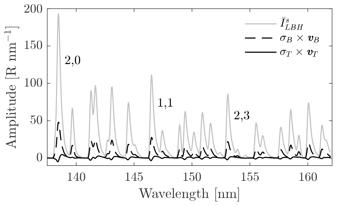
Figure 1 Simulated top-of-atmosphere mean LBH emissions (gray), ${\stackrel{\mathrm{‾}}{I}}_{\mathrm{LBH}}^{\mathrm{s}}$, and the principal components associated with overall brightening of emissions (dashed black), v_B, and the temperature signal (solid black), v_T, scaled by their respective eigenvalues, σ_B and σ_T. These two principal components account for 99.9 % of the variability about the mean for the period of 2–8 November 2018. The LBH emissions are generated with a spectral pixel size of 0.04 nm and a spectral resolution of 0.19 nm FWHM.

Figure 2 focuses on the LBH (2,0) band identified in Fig. 1. Compared to the other LBH bands the (2,0) band is relatively bright and is isolated from the even brighter atomic oxygen emissions at 130.4 and 135.6 nm and the atomic nitrogen emission at 149.3 nm (not shown in Fig. 1). The temperature signal in LBH emissions is apparent in the morphological shape of v_T displayed in Fig. 2. As the rotational temperature, T_r, of N₂ increases there is an effective skewing of the LBH (2,0) band to longer wavelengths. The close inspection of v_T indicates that LBH (2,0) band emissions at wavelengths above 138.56 nm are positively correlated with temperature while those below are negatively correlated. Emissions at 138.56 nm are not affected by temperature variability and thus have zero amplitude in v_T. This observation substantiates an approach of binning the LBH (2,0) band into two channels using 138.56 nm as a boundary to preserve how the temperature signal manifests in the LBH emission's morphological shape. Channel A is defined as the sum of all wavelengths negatively correlated with temperature ($\sum _{\mathit{\lambda }=\mathrm{138.0}}^{\mathrm{138.56}}{I}_{\mathit{\lambda }}$), and channel B contains all wavelengths positively correlated with temperature ($\sum _{\mathit{\lambda }=\mathrm{138.56}}^{\mathrm{139.2}}{I}_{\mathit{\lambda }}$). The two-channel ratio, $B/A$, is a linear function of temperature. A similar two-channel-ratio approach was adopted in Cantrall et al. (2019) for testing the feasibility of assimilating GOLD Level 1C data into the WAM, but a justification of such an approach was not provided.

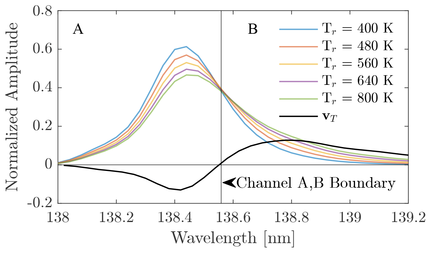
Figure 2 The second principal component (black line), v_T, over the LBH (2,0) band and the normalized amplitude of the LBH (2,0) band at five N₂ rotational temperatures, T_r. Emissions at 138.56 nm, where v_T changes the sign, are independent of temperature and provide a boundary to split the (2,0) band into channels A and B.

3 Determination of column-integrated temperature from the LBH (2,0) band

This section details the derivation of column-integrated thermospheric temperature, T_ci, from the N₂ rotational structure observed in top-of-atmosphere LBH emissions using the ratio of two channels that together span the LBH (2,0) band as motivated in Sect. 2. Section 3.1 explains the step-by-step procedure, followed by a discussion on potential error sources of T_ci in Sect. 3.2 and analysis in Sect. 3.3 that support the interpretation of T_ci as a column-integrated temperature rather than a temperature attributed to a specific altitude.

3.1 Procedure

The procedure to determine T_ci using the two-channel ratio consists of four steps as follows:

1. generate a set of synthetic LBH (2,0) bands at the instrument's spectral pixel size for a range of temperature using the vibrational–rotational band model (Budzien et al., 2001);

2. apply an instrument model on each synthetic band to account for the instrument's spectral resolution and spectral registration;

3. bin each band into channels A and B and fit the ratio, $B/A$, to temperature by least squares;

4. compute the ratio, $B/A$, from the observed LBH (2,0) band and determine T_ci by regressing the observed ratio on the predetermined relationship between the $B/A$ ratio and temperature.

The two-channel ratio has a number of benefits; most importantly, it can limit the impact of the following uncertainties: (1) uncertainty associated with LBH excitation and extinction processes that affect the absolute intensity of each band and (2) uncertainty associated with instrument performance variations across the LBH band system. This technique to derive T_ci only requires measurement of the relative magnitudes between two spectral channels (two spectral channels of size 0.5 nm) and a vibrational–rotational band model to map temperature to measurements. Measurement of a fully resolved, radiometrically calibrated LBH band system is not required and neither is a forward model to produce absolute LBH intensity.

3.2 Sources of error

There are two categories of error associated with determining physical parameters from observations: measurement error and representativeness error. The measurement error is the error associated with the measuring device, while the representativeness error is the difference between the observation and the physical model's representation of the observation (Rodgers, 2000). There are two dominant sources of systematic measurement error in T_ci stemming from variations in the instrument's spectral registration and resolution. Figure 3 shows the error in T_ci as a function of the error in the modeled spectral registration and the error in the modeled spectral resolution. It is apparent in Fig. 3 that a significant temperature error of about 50 K (5 %–10 %) can occur if the errors exceed a hundredth of a nanometer level for the spectral registration and a tenth of a nanometer level for spectral resolution. A discussion on mitigating these two sources of systematic measurement error when deriving T_ci from GOLD data is provided in Sect. 4.1.

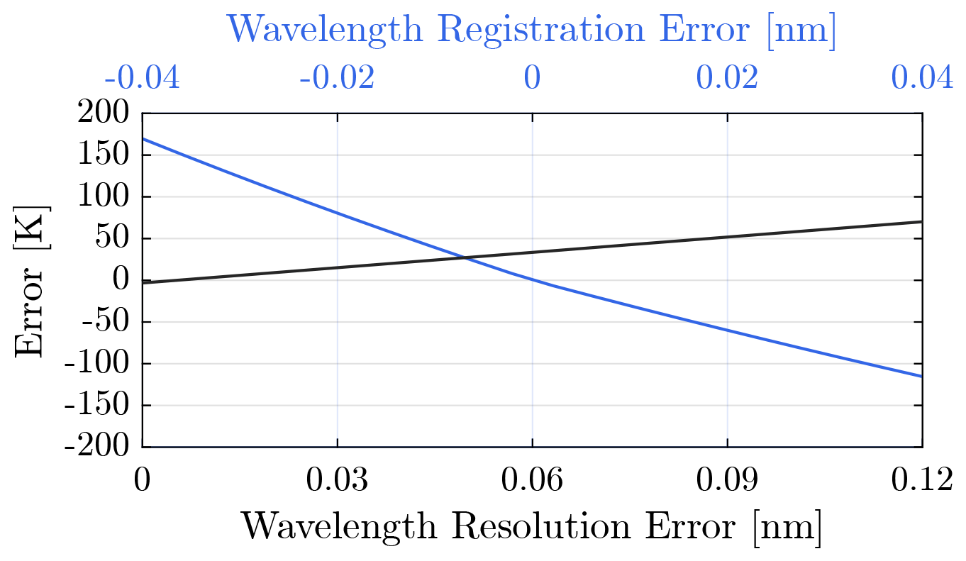
Figure 3 Expected bias errors in T_ci as a function of the two dominant known sources of systematic measurement errors: the instrument's spectral registration (blue) and variations in the spectral resolution (black).

The predominant source of random measurement error that determines the precision in T_ci is shot noise. The T_ci random measurement error due to shot noise is quantified using Monte Carlo samples of simulated T_ci derivations considering the instrument performance (McClintock et al., 2020a, b). Particle background counts are at times an additional random noise source. For the case study with GOLD data, the particle backgrounds were low as indicated by the “High_Background” flag in the Level 1C data, and therefore this error source is not considered. The statistics of background counts and the associated temperature errors should be quantified for the general application of this technique to any period.

Sources of representativeness error in deriving T_ci are those that cause relative differences in the channel intensity other than temperature that are not captured in the vibrational–rotational band model. Photoabsorption by O₂ is one source to consider. There is a 1.5 % difference in the mean O₂ absorption cross section between the two channels that corresponds to a negligible difference in transmittance along the line of sight considering the O₂ absorption cross-section variation with temperature. Another source of representativeness error associated with the (2,0) band is due to the overlap of the bright (2,0) transition and the weak (5,2) transition. Inaccurate specification of the v${}^{\prime }=\mathrm{2}$ and v${}^{\prime }=\mathrm{5}$ vibrational population rates cause a slight change in shape of the band with respect to the observations that could be interpreted as a change in the rotational temperature. Figure 8 in Ajello et al. (2020) provides the v${}^{\prime }=\mathrm{0}$–6 population rates and their uncertainties. These uncertainties are used to determine the associated error in the derived temperatures using the (2,0) band due to inaccurate specification of the v${}^{\prime }=\mathrm{2}$ and v${}^{\prime }=\mathrm{5}$ population rates. It is important to note that this representativeness error does not exist if the (1,1) or (2,3) bands are used in the derivation instead of the (2,0) band because the (1,1) and (2,3) bands are isolated from other LBH bands. However, these bands are also much weaker and suffer from significantly larger random error due to shot noise. Figure 4 shows the total random measurement error and representativeness error in T_ci using the (2,0) band. The representativeness error is a function of temperature and can range from 15 K at T_ci=400 to 48 K at T_ci=1200 K. Random measurement error from shot noise is a function of the (2,0) band intensity with values of 30 and 70 K for photon counts of 1500 and 250, respectively.

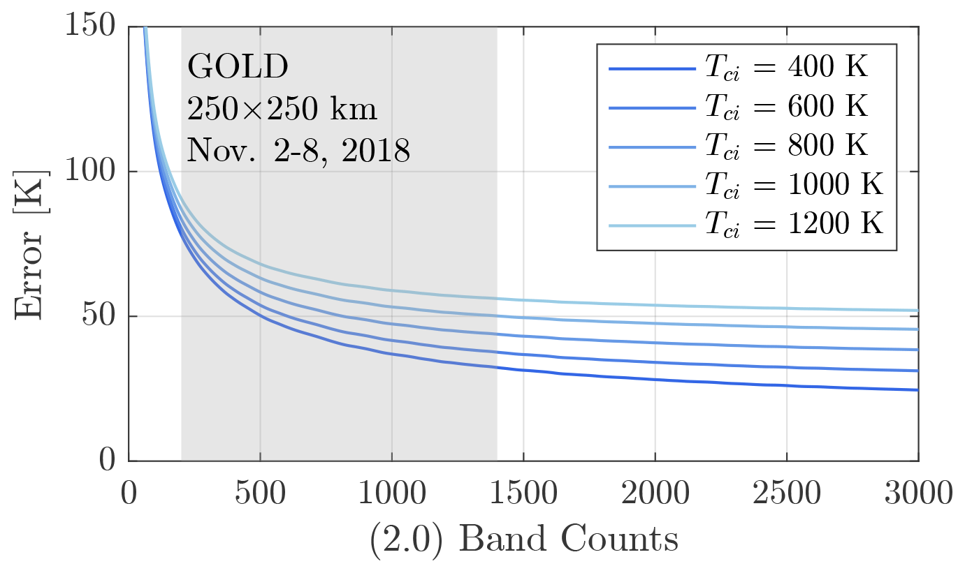
Figure 4 Total T_ci random measurement error (not including particle noise) and representativeness error for the (2,0) band. The range of (2,0) band counts for GOLD data (250×250 km resolution at nadir) used in the case study in Sect. 4 is highlighted by the gray box.

3.3 Interpretation of column-integrated temperature

Interpretation of column-integrated temperature, T_ci, is addressed using synthetic LBH disk emission observations generated by forward modeling WAM simulation results. The column-integrated temperature computed from synthetic observations is hereafter denoted as $T_{\mathrm{ci}}^{\mathrm{s}}$ to contrast to $T_{\mathrm{ci}}^{\mathrm{G}}$ computed from GOLD LBH disk emission data that is introduced later. To examine if $T_{\mathrm{ci}}^{\mathrm{s}}$ can be attributed to a certain pressure we compare the WAM pressure level with the temperature that most closely matches $T_{\mathrm{ci}}^{\mathrm{s}}$, denoted as $p_{T_{\mathrm{ci}}^{\mathrm{s}}}$, to the pressure level at the peak of the LBH contribution function, p_τ=1, where the LBH optical depth, τ, is unity. $p_{T_{\mathrm{ci}}^{\mathrm{s}}}$ and p_τ=1 are computed over the entire simulation period of 2–8 November 2018.

The LBH contribution function peak, p_τ=1, changes with solar zenith angle (SZA) and observing zenith angle (OZA) as shown in Fig. 5. p_τ=1 decreases in pressure (increases in altitude) for increases in SZA and OZA with a stronger dependence on SZA. Removing the OZA dependence, Fig. 6 shows there is a clear difference in p_τ=1 and $p_{T_{\mathrm{ci}}^{\mathrm{s}}}$ in their respective dependences on SZA ($p_{T_{\mathrm{ci}}^{\mathrm{s}}}$ ranges $\mathrm{3}\times {\mathrm{10}}^{-\mathrm{6}}$–$\mathrm{5}\times {\mathrm{10}}^{-\mathrm{6}}$ hPa and p_τ=1 ranges $\mathrm{2}\times {\mathrm{10}}^{-\mathrm{6}}$–$\mathrm{5.5}\times {\mathrm{10}}^{-\mathrm{6}}$ when SZA ranges 5–70^∘). The weaker SZA dependence of $p_{T_{\mathrm{ci}}^{\mathrm{s}}}$ can be explained by the FWHM of the contribution function that spans ∼60 km at low SZA and ∼90 km for high SZA (Laskar et al., 2021). The contribution function acts as an averaging kernel for temperature over these large vertical widths that tends to reduce the SZA effect. The net result is derived temperatures that are generally hotter than temperatures at p_τ=1 ($p_{T_{\mathrm{ci}}^{\mathrm{s}}}<p_{\mathit{\tau }=\mathrm{1}}$) for low SZA and temperatures that are generally cooler than temperatures at p_τ=1 ($p_{T_{\mathrm{ci}}^{\mathrm{s}}}>p_{\mathit{\tau }=\mathrm{1}}$) for high SZA. Figure 6 also shows variability in $p_{T_{\mathrm{ci}}^{\mathrm{s}}}$ (up to $\mathrm{1.5}\times {\mathrm{10}}^{-\mathrm{5}}$ hPa or ∼10 km for the simulation conditions) at a given SZA that reflects considerable variability in the vertical temperature structure within the width of the contribution function given varying forcing conditions.

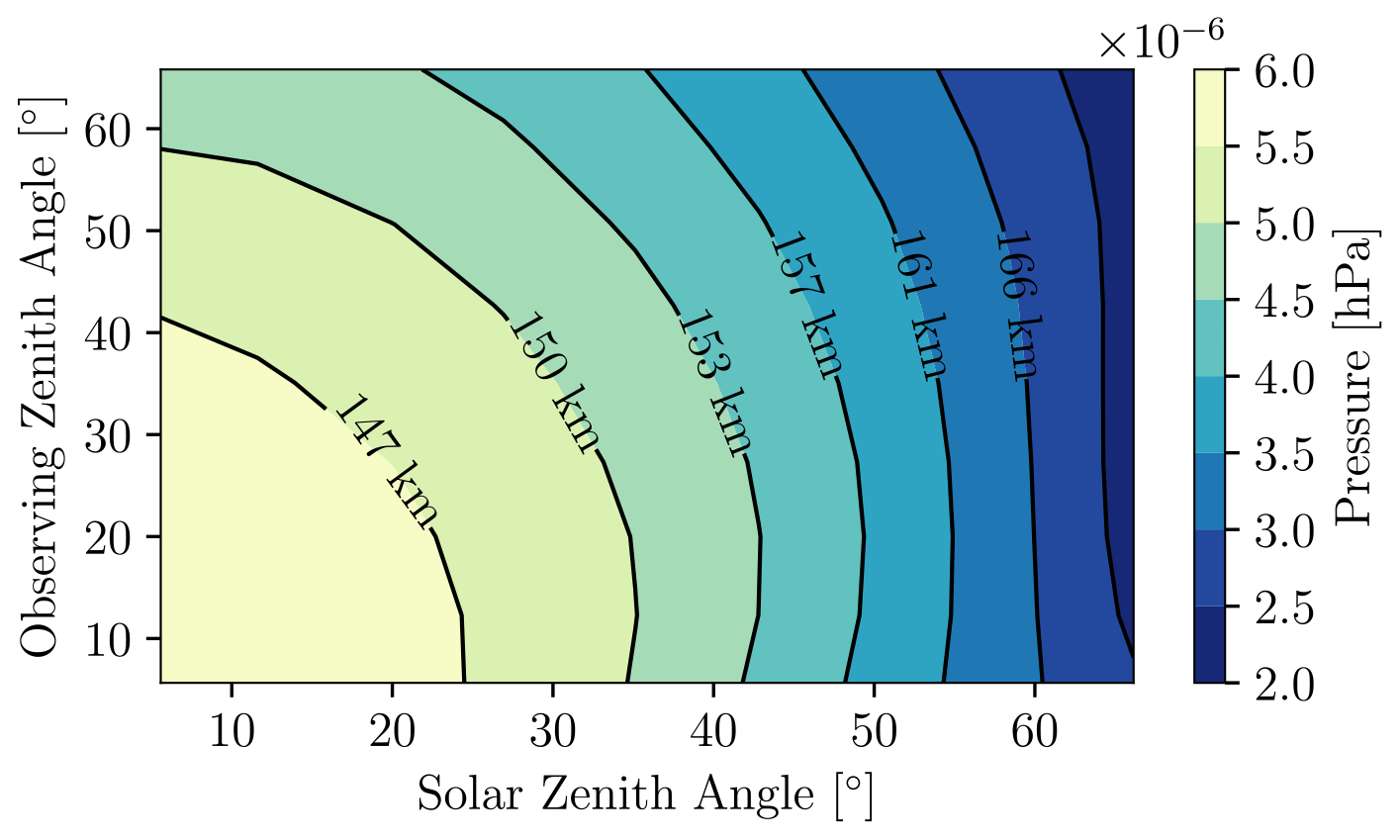
Figure 5 Pressure at the peak of the LBH contribution function, p_τ=1, as a function of SZA and OZA determined from forward modeling WAM simulations for the period of 2–8 November 2018 considering realistic forcing conditions. LBH emissions are on constant pressure level surfaces given SZA and OZA. Approximate corresponding altitudes in the WAM simulations are also provided, but note that these altitudes will vary depending on the forcing conditions.

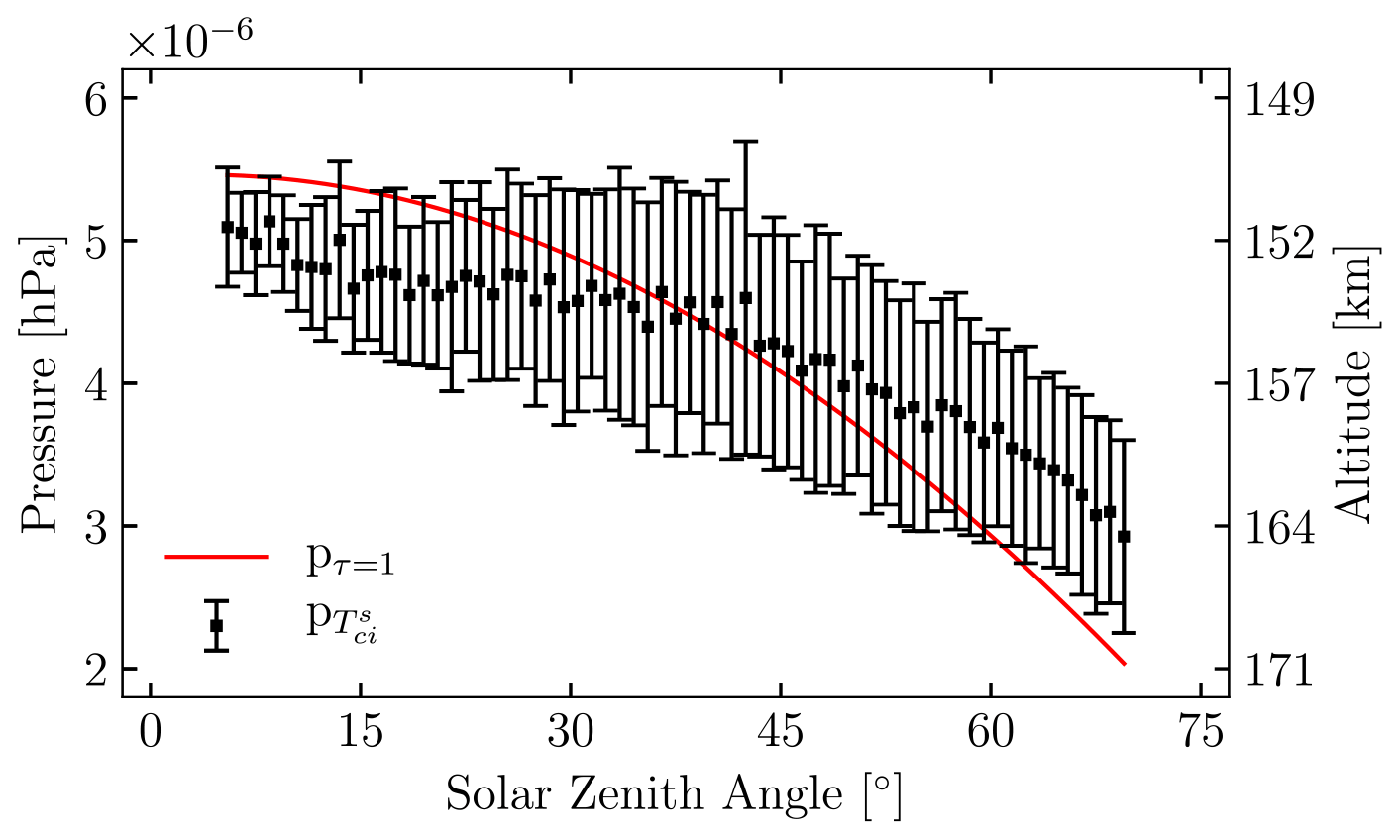
Figure 6 The mean and standard deviation of the pressure for the simulated WAM temperature that is closest to $T_{\mathrm{ci}}^{\mathrm{s}}$, $p_{T_{\mathrm{ci}}^{\mathrm{s}}}$, as a function of SZA averaged over all OZA for the simulation period of 2–8 November 2018 (black). The peak of the LBH contribution function, p_τ=1, is shown as a function of SZA based on forward modeling of LBH disk emissions using the same WAM simulation (red).

Figure 6 reinforces that T_ci derived from the procedural steps specified in Sect. 3.1 is a column-integrated quantity, containing information from a larger altitude range of the lower-middle thermosphere than just at p_τ=1. Perhaps, T_ci can be justified to be attributed to p_τ=1 when measurement and representativeness errors exceed the gap between T_ci and the temperatures at p_τ=1 at a given SZA and OZA. In general, specific pressure or altitude attribution of T_ci requires additional a priori knowledge of the thermospheric temperature profile.

Table 1 Variable definitions.

4 Case study

The two-channel-ratio approach to derive the column-integrated temperature is demonstrated using NASA GOLD Level 1C disk FUV emission data, $T_{\mathrm{ci}}^{\mathrm{G}}$, for the period of 2–8 November 2018 during which a moderate geomagnetic storm (Kp=5.8, $Dst=-\mathrm{55}$ nT) has occurred. Due to the lack of independent thermospheric temperature observations, the efficacy of this approach is validated through comparisons with GOLD Level 2 version 3 temperature product (T_DISK). $T_{\mathrm{ci}}^{\mathrm{G}}$ and T_DISK are equivalent variables only differing in their approach. $T_{\mathrm{ci}}^{\mathrm{G}}$ is also compared to two-channel column-integrated temperatures computed from the synthetic observations by forward modeling the WAM simulations ($T_{\mathrm{ci}}^{\mathrm{s}}$) as described in Sect. 2, along with two-channel column-integrated temperatures computed from synthetic observations by forward modeling NRLMSISE-00 (T_MSIS). The approach is further corroborated through comparisons of the storm-time changes of $T_{\mathrm{ci}}^{\mathrm{G}}$ to hemispherically integrated Joule heating rates (Q_JH) estimated from SuperDARN and ground-based magnetometer data using AMGeO, ESA SWARM mass density measurements at 460 km (${\mathit{\rho }}_{\mathrm{SWARM}}^{\mathrm{460}\mathrm{km}}$) based on calculation from precise orbit determinations using the Global Positioning System receivers on the spacecraft, and GOLD Level 2 version 3 $\mathrm{\Sigma }\mathrm{O}/{\mathrm{N}}_{\mathrm{2}}$ product ($\mathrm{\Sigma }{\mathrm{O}/{\mathrm{N}}_{\mathrm{2}}}^{\mathrm{G}}$). Section 4.1 provides a description of the GOLD LBH Level 1C disk emission data used in the $T_{\mathrm{ci}}^{\mathrm{G}}$ derivation; Sect. 4.2 presents results comparing $T_{\mathrm{ci}}^{\mathrm{G}}$ with T_DISK, T_MSIS, and $T_{\mathrm{ci}}^{\mathrm{s}}$; and Sect. 4.3 presents results comparing the storm-time response of $T_{\mathrm{ci}}^{\mathrm{G}}$ with Q_JH, ${\mathit{\rho }}_{\mathrm{SWARM}}^{\mathrm{460}\mathrm{km}}$, and $\mathrm{\Sigma }{\mathrm{O}/{\mathrm{N}}_{\mathrm{2}}}^{\mathrm{G}}$. Table 1 defines each of the variable symbols introduced above.

4.1 GOLD LBH disk emission data

GOLD observes the daytime FUV airglow from ∼134–162 nm on Earth's disk between 06:00 and 23:00 universal time (UT) from geostationary orbit at 47.5^∘ W longitude. A full disk image is produced every ∼30 min at a spatial resolution of 125×125 km by alternating between scans of the Northern Hemisphere and Southern Hemisphere. The GOLD Level 1C radiance data with a spectral pixel size of 0.04 nm are used to derive $T_{\mathrm{ci}}^{\mathrm{G}}$ in this study. The GOLD Level 1C data are spatially binned 2×2 (250×250 km spatial resolution) to improve the SNR by a factor of 2. Prior to deriving $T_{\mathrm{ci}}^{\mathrm{G}}$, efforts were made to reduce the impact of systematic biases that are present in version 3 of the GOLD Level 1C data product. Variations in spectral resolution along the GOLD detector are identified with the FWHM of the OI 135.6 doublet through fitting a 2-Gaussian distribution. Variations in the spectral registration are identified by differencing the modeled peak wavelength given the fitted OI 135.6 doublet FWHM by the peak wavelength determined by fitting a log-normal distribution to the (2,0) band. Note that the degradation of the detector due to the strength of the OI 135.6 doublet can cause errors in the spectral resolution estimate, but significant degradation had not occurred by 2–8 November 2018. Corrections for spectral registration and resolution are incorporated into Step 2 of the T_ci algorithm (see Sect. 3).

Figure 7 Comparison of $T_{\mathrm{ci}}^{\mathrm{G}}$ with T_DISK, T_MSIS, and $T_{{\mathrm{ci}}^{\mathrm{s}}}$ over Earth's disk viewed by GOLD from 3–7 November 2018 at about 15:00 UT, noon LT at the center of the disk (0^∘ N, 47.5^∘ W). A moderate geomagnetic storm (Kp=5.8, $Dst=-\mathrm{55}$ nT) commenced the evening of 4 November and lasted through 5 November.

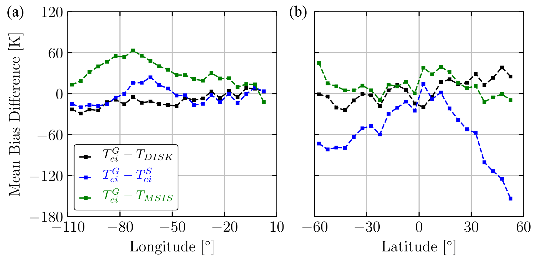
Figure 8 Mean bias difference (MBD) of $T_{\mathrm{ci}}^{\mathrm{G}}$ from T_DISK, T_MSIS, and $T_{{\mathrm{ci}}^{\mathrm{s}}}$ for 5^∘ bins as a function of longitude (a) and latitude (b) during 2–8 November 2018 at 15:00 UT. All longitudes viewed by GOLD are considered when computing MBD as a function of latitude, and only equatorial latitudes between ±10^∘ are considered when computing MBD as a function of longitude.

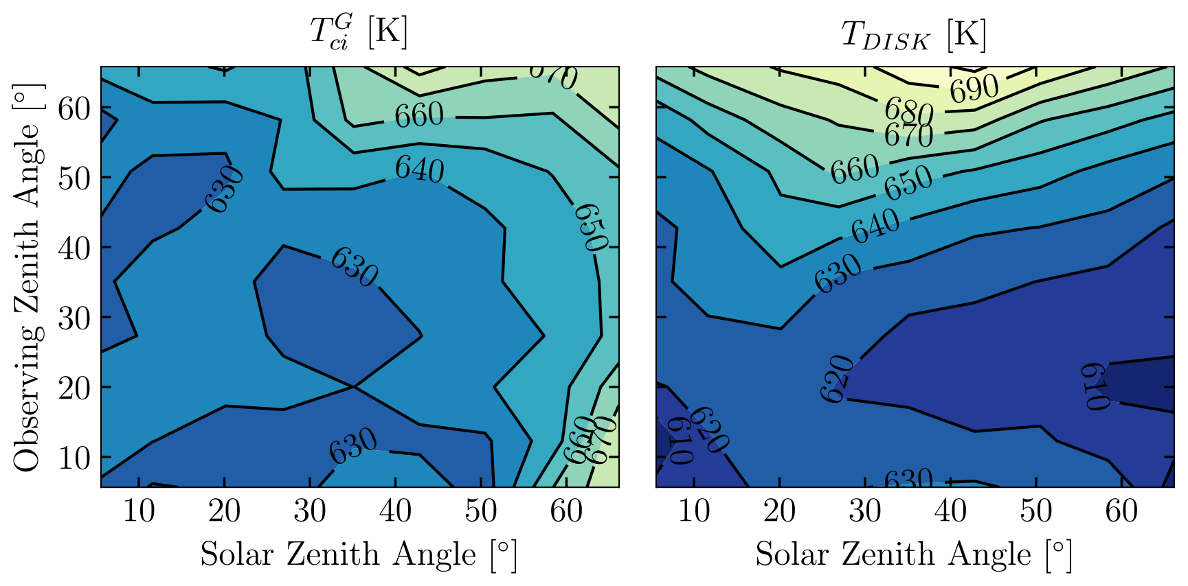
Figure 9 Mean $T_{\mathrm{ci}}^{\mathrm{G}}$ and T_DISK temperatures as a function of SZA and OZA for the period of 2–8 November 2018 with 5^∘ binning in SZA and OZA.

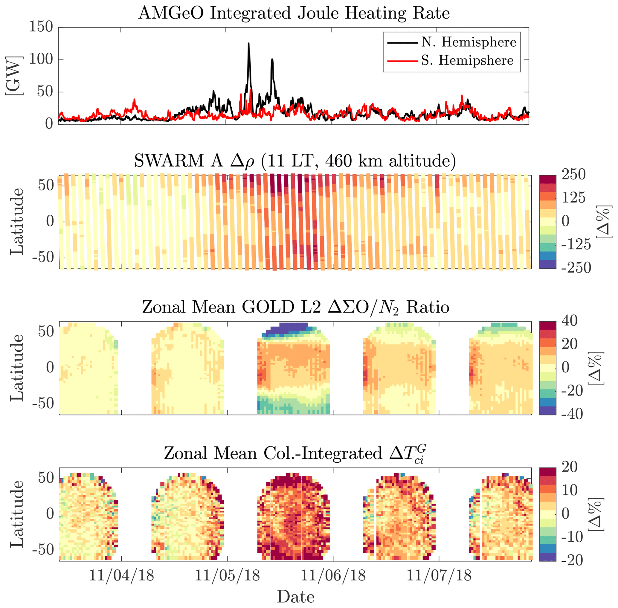
Figure 10 Storm-time response of the thermosphere as observed in three thermospheric variables as well as the hemispherically integrated Joule heating estimated using AMGeO. The percent change in mass density, ($\mathrm{\Delta }{\mathit{\rho }}_{\mathrm{SWARM}}^{\mathrm{460}\mathrm{km}}$), column $\mathrm{O}/{\mathrm{N}}_{\mathrm{2}}$ ratio ($\mathrm{\Delta }\mathrm{\Sigma }\mathrm{O}/{\mathrm{N}}_{\mathrm{2}}$), and column-integrated temperature ($\mathrm{\Delta }{T}_{\mathrm{ci}}^{\mathrm{G}}$) are computed with quiet-time conditions on 2 November 2018.

4.2 Comparing $T_{\mathrm{ci}}^{\mathrm{G}}$ to T_DISK, T_MSIS, and $T_{\mathrm{ci}}^{\mathrm{s}}$

Figure 7 displays $T_{\mathrm{ci}}^{\mathrm{G}}$ along with T_DISK, T_MSIS, and $T_{\mathrm{ci}}^{\mathrm{s}}$ over Earth's disk viewed by GOLD from 3–7 November 2018 at 15:00 UT, noon local time (LT) at the center of the disk (0^∘ N, 47.5^∘ W). A moderate geomagnetic storm commenced the evening of 4 November and lasted through 5 November (Gan et al., 2020). Figure 8 shows the mean bias difference (MBD) of $T_{\mathrm{ci}}^{\mathrm{G}}$ from T_DISK, T_MSIS, and $T_{\mathrm{ci}}^{\mathrm{s}}$ as a function of longitude (considering latitudes between ±10^∘) and latitude (considering all longitudes viewed by GOLD) for 2–8 November 2018 at 15:00 UT. During this period the temperatures derived from observations (i.e., $T_{\mathrm{ci}}^{\mathrm{G}}$ and T_DISK) exhibit globally similar temperature amplitudes and display a similar morphological temperature response to geomagnetic activity over the disk. Note that there is slight banding near the Equator in $T_{\mathrm{ci}}^{\mathrm{G}}$ and T_DISK where the Southern Hemisphere and Northern Hemisphere scans meet that is likely due to systematic errors at the top and bottom edge of the detector that were not completely corrected. $T_{\mathrm{ci}}^{\mathrm{G}}$ and T_DISK show strong agreement near the center of the disk with an MBD less than 15 K (1 %–3 %) increasing to a maximum of ∼40 K (4 %–8 %) near the disk edge. The slope of $T_{\mathrm{ci}}^{\mathrm{G}}$–T_DISK with respect to latitude and longitude indicates $T_{\mathrm{ci}}^{\mathrm{G}}$ has a stronger south–north and west–east temperature gradient than T_DISK. There is also agreement in the temperature morphology over the disk between $T_{\mathrm{ci}}^{\mathrm{G}}$ and $T_{\mathrm{ci}}^{\mathrm{s}}$ prior to the storm, but the storm-time response simulated by WAM, as manifest in $T_{\mathrm{ci}}^{\mathrm{s}}$, shows considerably higher temperatures in the mid- and high latitudes and a longer post-storm recovery time in comparison to $T_{\mathrm{ci}}^{\mathrm{G}}$ and T_DISK. $T_{\mathrm{ci}}^{\mathrm{G}}$–$T_{\mathrm{ci}}^{\mathrm{s}}$ displays a similar west–east slope to $T_{\mathrm{ci}}^{\mathrm{G}}$–T_DISK except for the region just west of the sub-solar point (−80 to −50^∘ longitude) where $T_{\mathrm{ci}}^{\mathrm{s}}$ is ∼25 K cooler than $T_{\mathrm{ci}}^{\mathrm{G}}$. T_MSIS and $T_{\mathrm{ci}}^{\mathrm{G}}$ show agreement in the temperature morphology over the disk, but T_MSIS displays cooler temperatures, particularly just west of the subsolar point at low and mid-latitudes (up to 60 K), and a stronger west–east temperature gradient.

The $T_{\mathrm{ci}}^{\mathrm{G}}$ and T_DISK comparison is expanded in Fig. 9 to include all times in the range 07:00–22:00 UT for the period of 2–8 November 2018. Figure 9 shows that $T_{\mathrm{ci}}^{\mathrm{G}}$ and T_DISK have different behavior with the viewing conditions determined by SZA and OZA. $T_{\mathrm{ci}}^{\mathrm{G}}$ increases with both SZA and OZA with a stronger trend for SZA. T_DISK increases with OZA but remains relatively uniform with SZA, even decreasing slightly for SZA > 25^∘. There are two likely explanations for the dependence of the derived temperatures on viewing conditions: (1) the derived temperatures reflect real temperature changes with viewing conditions because the contribution function is peaking at different pressures (Fig. 5); (2) the derived temperatures reflect temperature biases with viewing conditions because the LBH emission intensity is changing. Intensity decreases with increasing SZA due to reduced LBH excitation but increases with increasing OZA due to a larger air mass along the line of sight. To test which explanation best describes the dependence of $T_{\mathrm{ci}}^{\mathrm{G}}$ and T_DISK on viewing conditions, Fig. 9 is correlated to the pressure at the peak of the LBH contribution function, p_τ=1, (Fig. 5) and to the mean LBH intensity measured by GOLD over the same period as a function of SZA and OZA. T_DISK is weakly correlated ($R=-\mathrm{0.15}$) with p_τ=1 and strongly correlated (R=0.72) with LBH intensity. In contrast, $T_{\mathrm{ci}}^{\mathrm{G}}$ is strongly correlated ($R=-\mathrm{0.86}$) with p_τ=1 and weak-moderately correlated ($R=-\mathrm{0.32}$) with LBH intensity. The stronger correlation between $T_{\mathrm{ci}}^{\mathrm{G}}$ and p_τ=1 compared to T_DISK and p_τ=1 and weaker correlation between $T_{\mathrm{ci}}^{\mathrm{G}}$ and LBH intensity compared to T_DISK and LBH intensity over this analysis period is suggestive that $T_{\mathrm{ci}}^{\mathrm{G}}$ is more sensitive to real temperature changes as the probed pressures change with viewing conditions and less susceptible to biases due to a change in LBH intensity with viewing conditions. This is attributed to the fact that $T_{\mathrm{ci}}^{\mathrm{G}}$ derivation does not require measurement of a fully resolved, radiometrically calibrated LBH band system nor a forward model to produce absolute LBH intensity. There are likely still biases in $T_{\mathrm{ci}}^{\mathrm{G}}$ with LBH intensity as indicated by the weak-moderate correlation ($R=-\mathrm{0.32}$), particularly at low intensities (high SZA) where shot noise can lead to positive biases up to 15 K in the two-channel-ratio approach.

4.3 Storm-time response

Figure 10 displays the response to the geomagnetic storm in $T_{\mathrm{ci}}^{\mathrm{G}}$, Q_JH, ${\mathit{\rho }}_{\mathrm{SWARM}}^{\mathrm{460}\mathrm{km}}$, and $\mathrm{\Sigma }{\mathrm{O}/{\mathrm{N}}_{\mathrm{2}}}^{\mathrm{G}}$. $T_{\mathrm{ci}}^{\mathrm{G}}$, ${\mathit{\rho }}_{\mathrm{SWARM}}^{\mathrm{460}\mathrm{km}}$, and $\mathrm{\Sigma }{\mathrm{O}/{\mathrm{N}}_{\mathrm{2}}}^{\mathrm{G}}$ are shown as percent differences from the quiet-time conditions on 2 November 2018. The global temporal evolution of these variables is in good agreement with each other and consistent with known storm-time responses of thermospheric variables (e.g., Fuller-Rowell et al., 1994). A rise of magnetospheric energy influx as suggested by Q_JH leads to increased temperatures and upwelling of heavy molecular-rich air in the high and mid-latitudes as indicated by depletions of $\mathrm{\Sigma }{\mathrm{O}/{\mathrm{N}}_{\mathrm{2}}}^{\mathrm{G}}$ (−40 % near 50^∘ latitude and −20 % near −50^∘ latitude) and enhancements of $T_{\mathrm{ci}}^{\mathrm{G}}$ (∼20 % near ±50^∘ latitude) and ${\mathit{\rho }}_{\mathrm{SWARM}}^{\mathrm{460}\mathrm{km}}$ (∼250 % near ±50^∘ latitude). Enhancements of $\mathrm{\Sigma }{\mathrm{O}/{\mathrm{N}}_{\mathrm{2}}}^{\mathrm{G}}$ (20 %–30 % near 30^∘ latitude) in the low latitudes suggest a subsequent development of downwelling following the pole-to-Equator global circulation in response to the storm-time Joule heating rise. Global thermospheric expansion is also apparent on 5 November as suggested by an increase in $T_{\mathrm{ci}}^{\mathrm{G}}$ and ${\mathit{\rho }}_{\mathrm{SWARM}}^{\mathrm{460}\mathrm{km}}$ over all latitudes. Note that the first detection of the temperature change was on the evening of 4 November when Joule heating rates have started to increase but are still relatively low (<50 GW). The post-storm recovery times are also in good agreement and appear to be on the order of 2–3 d.

5 Conclusions

A new technique to derive thermospheric temperature from space-based disk observations of FUV airglow is presented. The technique uses a ratio of the emissions in two spectral channels that together span the Lyman–Birge–Hopfield (LBH) (2,0) band to determine the change in band shape with respect to a change in the rotational temperature of N₂. While this study focused on the LBH (2,0) band to derive thermospheric temperature, the described technique can be applied to any LBH band or combination of bands. The derived temperature from this technique is shown to be a column-integrated property referred to as column-integrated thermospheric temperature, T_ci. T_ci should not be attributed to the peak of the LBH contribution function without consideration of the viewing conditions and T_ci derivation uncertainty. The definition of column-integrated thermospheric temperatures and other parameters used for comparison in the paper is given in Table 1. Specific findings of this work are as follows.

The LBH spectrum quantified with PCA of synthetic daytime LBH disk emission data is found to be highly compressible (two principal components explain 99.9 % of the variability). Analysis of the secondary principal component mode, which characterizes how the LBH temperature signal manifests as the change in band shape, substantiates the approach to bin an LBH spectral band into two channels such that the temperature-induced band shape change is best preserved. The study has shown that thermospheric temperatures can be derived from an observed two-channel ratio by using a precomputed relationship of the ratio to temperature from an LBH vibrational–rotational band model. In this two-channel-ratio approach, representativeness errors originating from forward modeling are reduced because radiometrically calibrated LBH band intensities are not required in the derivation procedure, and negative impacts of systematic measurement errors, stemming from variations across the band system in the instrument's spectral registration and resolution, are reduced because a fully resolved LBH band system is not required.

The derived temperature from the two-channel approach can have significant systematic biases of about 50 K (5 %–10 %) if the spectral registration and resolution are not known to the hundredth of a nanometer level and tenth of a nanometer level, respectively, as shown in Fig. 3. In addition to these known sources of systematic biases, there is intrinsic random error in T_ci due primarily to shot noise and representativeness error due to misspecification of the $v^{\prime }=\mathrm{2}$ and $v^{\prime }=\mathrm{5}$ population rates in the vibrational–rotational band model. The random measurement error is estimated to be 20–60 K (3 %–9 %), and the representativeness error is estimated to be 15–30 K (2 %–5 %) for the case study with GOLD L1C data.

For the period of 2–8 November 2018 during which a moderate geomagnetic storm has occurred, the temperatures derived from observations (i.e., $T_{\mathrm{ci}}^{\mathrm{G}}$ and T_DISK) exhibit globally similar temperatures. $T_{\mathrm{ci}}^{\mathrm{s}}$ is in good agreement with $T_{\mathrm{ci}}^{\mathrm{G}}$ and T_DISK at low latitudes but exhibits considerably higher temperatures at mid- and high latitudes during the storm response. T_MSIS exhibits globally cooler temperatures to the observations. However, there are clear differences between $T_{\mathrm{ci}}^{\mathrm{G}}$ and T_DISK with respect to viewing conditions. There is stronger correlation between $T_{\mathrm{ci}}^{\mathrm{G}}$ and p_τ=1 ($R=-\mathrm{0.86}$) compared to T_DISK and p_τ=1 ($R=-\mathrm{0.14}$) and weaker correlation between $T_{\mathrm{ci}}^{\mathrm{G}}$ and LBH intensity ($R=-\mathrm{0.32}$) compared to T_DISK and LBH intensity (R=0.72) over the analysis period. These differences highlight a potential benefit of the two-channel-ratio approach to reduce the representativeness error by measurement of the relative intensities between two channels that only requires a vibrational–rotational band model for the forward model instead of a full radiative transfer model. The temporal evolution of global T_ci corroborates well with temporal changes of hemispherically integrated Joule heating rates Q_JH, SWARM mass density at 460 km ${\mathit{\rho }}_{\mathrm{SWARM}}^{\mathrm{460}\mathrm{km}}$, and GOLD $\mathrm{\Sigma }{\mathrm{O}/{\mathrm{N}}_{\mathrm{2}}}^{\mathrm{G}}$, which is consistent with known storm-time responses of thermospheric variables.