the Creative Commons Attribution 4.0 License.
the Creative Commons Attribution 4.0 License.
 | 07 Dec 2021
Retrieval algorithm for OClO from TROPOMI (TROPOspheric Monitoring Instrument) by differential optical absorption spectroscopy
Jānis Puķīte
Christian Borger
Steffen Dörner
Myojeong Gu
Udo Frieß
Andreas Carlos Meier
Carl-Fredrik Enell
Uwe Raffalski
Andreas Richter
Thomas Wagner
Here we present a new retrieval algorithm of the slant column densities (SCDs) of chlorine dioxide (OClO) by differential optical absorption spectroscopy (DOAS) from measurements performed by TROPOspheric Monitoring Instrument (TROPOMI) on board of Sentinel-5P satellite. To achieve a substantially improved accuracy, which is especially important for OClO observations, accounting for absorber and pseudo absorber structures in optical depth even of the order of 10−4 is important. Therefore, in comparison to existing retrievals, we include several additional fit parameters by accounting for spectral effects like the temperature dependency of the Ring effect and Ring absorption effects, a higher-order term for the OClO SCD dependency on wavelength and accounting for the BrO absorption.
We investigate the performance of different retrieval settings by an error analysis with respect to random variations, large-scale systematic variations as a function of solar zenith angle and also more localized systematic variations by a novel application of an autocorrelation analysis.
The retrieved TROPOMI OClO SCDs show a very good agreement with ground-based zenith sky measurements and are correlated well with preliminary data of the operational TROPOMI OClO retrieval algorithm currently being developed as part of ESA's Sentinel-5P+ Innovation project.
- Article
(42406 KB) - Full-text XML
- Companion paper
- BibTeX
- EndNote


It is well known that catalytic halogen chemistry causes large depletion of ozone in polar regions in spring (WMO, 2018). In particular, Cl2 is released in large amounts by heterogeneous reaction of ClONO2 and HCl on polar stratospheric clouds (PSCs). Once the air mass with Cl2 becomes irradiated by sunlight, Cl2 is subsequently photolysed to atomic Cl (Solomon et al., 1986). Atomic Cl can also result from other reactions such as between ClONO2 and liquid- or solid-phase H2O and subsequent photolysis of the produced HOCl or other reactions as very recently pointed out by Nakajima et al. (2020). Atomic Cl in turn reacts with ozone (Stolarski and Cicerone, 1974). Because the resulting ClO (with or without involvement of BrO) is returned to atomic Cl (Molina and Molina, 1987; McElroy et al., 1986) by further reactions, a very effective ozone depletion process takes place. Furthermore, chlorine dioxide (OClO) is a possible outcome of a reaction between ClO and BrO (Sander and Friedl, 1989):
The dominant loss mechanism for atmospheric OClO is its very rapid photolysis (Solomon et al., 1990):
which results in a null cycle with respect to ozone loss by recycling odd oxygen. Thus, OClO can be used as an indicator for halogen chemistry because of the nearly linear dependence of OClO formation to ClO and BrO concentrations (Schiller and Wahner, 1996) at high solar zenith angles (SZAs) where the photolysis is slow enough to provide OClO abundances above the detection limit for the passive scattered light UV–Vis measurements (Solomon et al., 1987). Measurements of OClO in the context of the passive scattered light UV–Vis measurements became of special interest when Solomon et al. (1987) measured it first in Antarctica. OClO has well-structured absorption features in the near UV (Wahner et al., 1987) which can be detected by differential optical absorption spectroscopy (DOAS) (Platt and Stutz, 2008).
First satellite retrievals of OClO were enabled by measurements by the GOME-1 (Global Ozone Monitoring Experiment) instrument launched in 1995, consequently leading to many studies investigating the polar stratospheric chlorine activation (Burrows et al., 1999; Wagner et al., 2001, 2002b; Kühl et al., 2004a, b; Richter et al., 2005). Later, also measurements by SCIAMACHY, OSIRIS, OMI or GOME-2 were available for analysis (Kühl et al., 2006; Krecl et al., 2006; Kühl et al., 2008; Puķīte et al., 2008; Oetjen et al., 2011; Hommel et al., 2014).
The TROPOspheric Monitoring Instrument (TROPOMI) is a UV–Vis–NIR–SWIR nadir-viewing instrument on board of the Sentinel-5P satellite developed for monitoring the Earth's atmosphere (Veefkind et al., 2012). It was launched on 13 October 2017 in a near-polar orbit. It measures spectrally resolved earthshine radiances at an unprecedented spatial resolution of around 3.5×7.2 km2 (near nadir) at a high signal-to-noise ratio. The measurements are performed via a push-broom spectrometer consisting of 450 detector rows. It has a total swath width of ∼2600 km on the Earth's surface, providing daily global coverage. The spatial resolution has been further increased to 3.5×5.6 km2 (near nadir) starting from 6 August 2019 (Rozemeijer and Kleipool, 2019).
In this paper we present a new retrieval algorithm for slant column densities (SCDs) of OClO by applying the DOAS method to TROPOMI measurements. The article is structured as follows. In Sect. 2 we present the TROPOMI OClO retrieval algorithm, while in Sect. 3 we compare the results with ground-based zenith sky measurements obtained during polar Arctic winters in Kiruna, Sweden, and Antarctic winters in Neumayer III, Antarctica. Section 4 correlates the retrieved OClO SCDs with preliminary data of the TROPOMI OClO retrieval algorithm currently being developed as part of ESA's Sentinel-5P+ Innovation (S5P+I) project. Finally, Sect. 5 draws some conclusions.
The principle of the DOAS method (Platt and Stutz, 2008) is based on the application of the Beer–Lambert law by performing a least squares fit to best scale the contributions of the fit parameters to the measured optical depth (logarithmic normalized intensity):
where I and I0 are radiances of the measurement and reference (or Fraunhofer) spectra, respectively. Si is a scaling factor of constituent i, and σi(λ) is its wavelength-dependent cross section. P is a broadband spectral contribution due to light scattering approximated by a polynomial. In the first place, scaling factor Si describes trace gas slant column densities (SCDs), habitually interpreted as number densities of trace gases integrated along their effective light paths. Besides that, also other parameters, scaling linearly in optical depth space, that as approximations account for additional spectral features with corresponding pseudo cross sections, can and, depending on circumstances, should be included in the fit. They can include, but are not limited to, the Ring effect (Wagner et al., 2009), offset correction, shift and stretch (Rozanov et al., 2011; Beirle et al., 2013), tilt effect (Rozanov et al., 2011; Lampel et al., 2017), polarization corrections (McLinden et al., 2002; Kühl et al., 2006), changes in the instantaneous spectral response function (ISRF) with respect to the ISRF obtained during calibration (Beirle et al., 2017) or higher-order contributions to account for non-linearities in absorption, and SCD dependency on scattering (Puķīte et al., 2010; Puķīte and Wagner, 2016).
SCDs obtained from measurements in the limb mode (vertical scanning of the atmosphere with the instrument pointing above the Earth's horizon as done by OSIRIS and SCIAMACHY) can be converted to vertical OClO concentration profiles (Krecl et al., 2006; Kühl et al., 2008) or even 2D vertical concentration fields along the orbit by means of a tomographic approach (Puķīte et al., 2008). For nadir measurements, SCDs can be converted to vertical column densities (VCDs, vertical integrals of number density profiles) by applying radiative transfer modelling (Solomon et al., 1987; Wagner et al., 2001; Kühl et al., 2004a). However, it is often preferred to omit this step for nadir measurements of OClO mainly because of two reasons (Kühl et al., 2004a). First, for the radiative transfer simulations, the atmospheric state must be well known (especially at high SZAs (≳85∘) which are of special interest for OClO), including the OClO profile which is highly variable due to the large photochemical reactivity (Solomon et al., 1990). Second, the OClO VCDs at these high SZAs cannot be interpreted as a measurement of chlorine activation level, since they still depend on the photolysis rate of OClO, which in turn strongly depends on the intensity of solar illumination and thereby also on the SZA (Kühl et al., 2004a). In other words, the calculation of the VCD at a given location would necessarily require a priori constrains about the concentration variability along the light path. Therefore, this study also limits the retrieval to SCDs.
(Beirle et al., 2017)(Kromminga et al., 2003)(Vandaele et al., 1998)(Serdyuchenko et al., 2014)(Thalman and Volkamer, 2013)(Puķīte and Wagner, 2016)(Beirle et al., 2013)(Beirle et al., 2017)(Warnach et al., 2019)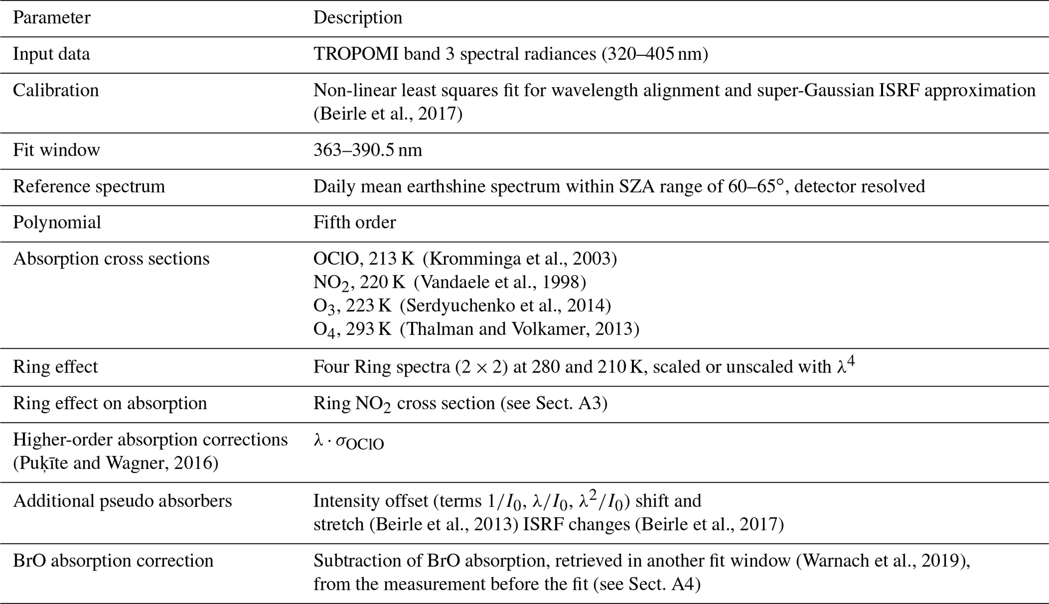
2.1 Retrieval settings
The retrieval of the OClO SCDs is performed by a universal fit routine which was originally developed for the TROPOMI water vapour retrieval (Borger et al., 2020). Retrieval parameters for OClO are provided in Table 1.
Before the application of the DOAS method, a spectral calibration is performed for each of the TROPOMI rows separately to obtain measurement wavelength grids and ISRFs. The calibration includes a non-linear least-squares fit in intensity space with respect to a high-resolution solar spectrum (Kurucz et al., 1984) for wavelength alignment and slit function determination approximated by an asymmetric super-Gaussian function as described by Beirle et al. (2017). The calibration is done for the reference spectrum (I0) for which in our application we take a daily mean of the normalized earthshine measurements within a solar zenith angle range of 60–65∘ as defined in Appendix A1.2. The normalization is done for each spectrum by its maximum spectral intensity value within the evaluated spectral range. Cross sections of ozone and NO2 are considered in the calibration fit to account for absorption in the earthshine reference. The usage of an earthshine reference is motivated by the need to reduce detector-related effects (e.g. Wagner et al., 2001; Kühl et al., 2006), in particular the detector striping and the amplitude of the Ring effect, which are both more prominent when direct Sun measurements are used. The use of an earthshine reference does not hinder the interpretation of the retrieved OClO data, because no OClO is expected to be found at these low SZAs. It is hence expected that the mean of the retrieved OClO slant column densities in the reference region is zero. The use of the normalized spectra (Appendix A1.2) for the calculation of the daily mean (at practically no additional calculation effort) also ensures that spectral features that are not related to OClO but correlate with its cross section are not producing an artificial offset. However, the effect of this theoretically better approach for this application is negligible.
The DOAS analysis is performed within a fit window from 363 to 390.5 nm. Absorption cross sections of OClO at 213 K (Kromminga et al., 2003), NO2 at 220 K (Vandaele et al., 1998), O3 at 223 K (Serdyuchenko et al., 2014) and O4 at 293 K (Thalman and Volkamer, 2013) are included in the fit. P is approximated by a fifth-order polynomial. For the convolution of the cross sections to the instrument spectral resolution, an intensity-weighted convolution (to account for I0 correction) is applied as described in Appendix A2 (Eq. A9).
In the fit we also account for the intensity offset, shift and stretch (Beirle et al., 2013), and ISRF parameter changes (Beirle et al., 2017). The Ring effect is accounted for by Ring spectra calculated at two temperatures (280 and 210 K) in order to account for the dependency of the Ring spectra on temperature, which we found is important (see Appendix B9). The two Ring spectra are calculated from the earthshine reference spectrum and included in the fit. Also, each is scaled with λ4 according to Wagner et al. (2009) (additional two spectra included in the fit). The use of an earthshine reference spectrum for the calculation of the Ring spectrum is in accordance with previous studies (e.g. Kühl et al., 2004b, 2006, 2008) and is found to give an improvement with respect to the calculation of the Ring spectra from measured Sun irradiance spectra.
Also a λ⋅σOClO term according to the approach by Puķīte et al. (2010) and Puķīte and Wagner (2016) (convolved with intensity-weighted convolution, Eq. A11) is included in the fit. Besides its physical meaning to account for the broadband wavelength dependency of the OClO SCD due to the change of light path distribution in the atmosphere, which is large at high SZAs, this parameter gives more flexibility to better account for the parameter cross-correlation problem, because one can calculate the final OClO SCD at a wavelength which is less affected by systematic errors caused by the imperfection of the model.
The retrieved OClO SCDs are obtained from the fitted quantities according to the formalism in Puķīte and Wagner (2016) by
where SOClO,σ is the fit result corresponding to the OClO cross section, and SOClO,λσ is for the λ⋅σOClO term. λ=379 nm is selected for the evaluation because this wavelength provides a good trade-off between precision and accuracy (see also the sensitivity studies in Appendices B1 and B2).
Additionally, a cross section is added to approximate the impact due to the Ring effect on the NO2 absorption. This NO2 Ring absorption spectra term accounts for the first-order NO2 absorption contribution of the Raman scattered light. The definition is provided in Appendix A3. It also turned out to be advantageous to correct the measured spectra prior to the OClO DOAS fit for the BrO absorption, because we found an interference of the retrieved OClO SCDs towards BrO. However, inclusion of BrO cross section as an additional fit parameter led to even larger systematic errors. Therefore, a BrO correction (with the BrO absorption determined in a different spectral range) is applied before the OClO retrieval on the measured spectra as described in Appendix A4.
2.2 Retrieval performance and spatial data binning
Uncertainties in passive scattered light DOAS measurements depend on retrieval noise, the accuracy of the removal of Fraunhofer bands, the absorption cross sections, unexplained spectral structures and effects of the radiative transfer (Platt and Stutz, 2008). For the OClO cross section by Wahner et al. (1987), systematic errors (≤8 %) could be due to the absolute calibration (Wagner et al., 2001). For the cross section used in this study, Kromminga et al. (2003) stated that their cross sections agree with those by Wahner et al. (1987) within a similar error range. Thus, we assume a similar error (∼10 %). In the following the retrieval performance is investigated by means of a statistical analysis. While the impact of the retrieval settings is studied in Appendix B, it is also summarized in the following (Sect. 2.2.4), motivating the retrieval setup we introduced in Sect. 2.1.
2.2.1 Systematic and random errors
In order to determine the contribution of systematic errors, we make use of the fact that OClO occurs only for limited time periods and areas. Thus, we investigate the retrieved OClO SCDs for scenes where no OClO absorption is expected. This allows one to investigate the retrieval performance by means of a statistical analysis. The left panel in Fig. 1 shows daily means of retrieved OClO SCDs for 3 d in each hemisphere binned on a SZA grid with a bin size of 0.2∘. The days are selected to represent different atmospheric conditions at different time periods. For the Northern Hemisphere (NH) and Southern Hemisphere (SH), 25 August 2018 and 25 December 2018 are summer days in the respective hemispheres when no enhanced OClO SCDs are expected. The dates 25 November 2018 (NH) and 25 April 2019 (SH) are early winter days with temperatures not yet having dropped below the PSC-forming temperature; thus, again no enhanced OClO SCDs are expected. The date 25 December 2018 (NH) is an example of a day with enhanced OClO concentrations present; the level, however, is low as is the case in this winter. The date 25 August 2018 (SH) shows typical OClO values for the Antarctic winter atmosphere with a very strong chlorine activation. The right panel in Fig. 1 illustrates the standard deviation of the OClO SCDs, a measure we use for the mean random error.
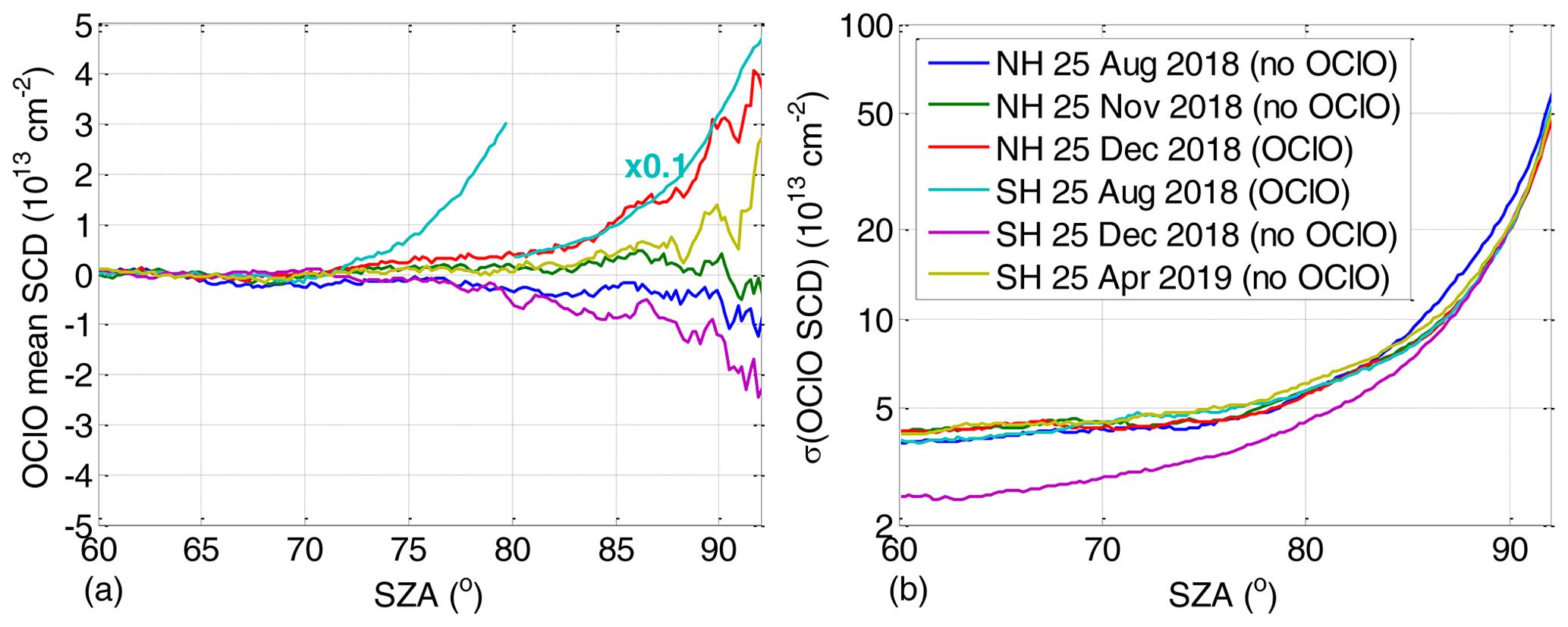
Figure 1(a) OClO mean SCDs resolved on 0.2∘ SZA grid for 3 d indicated in the legend on the right in different seasons for each hemisphere. It is also indicated which days are expected to have enhanced OClO. Note that the SCDs as plotted for 25 August 2018 in the SH are multiplied by the factor of 0.1 for SZAs above 80∘. (b) Same but standard deviation of OClO SCDs.
Both the retrieved mean OClO SCDs and their standard deviations show a pronounced increase with increasing SZA. The increase in the standard deviations can be expected due to a lower signal-to-noise ratio at twilight. Considering the days for which no enhanced OClO SCDs are expected, the daily mean OClO (or systematic offset with respect to the expected zero) is largest for SH being around 1×1013 cm−2 where the offset sign is different between December and April.
The standard deviation at the same time is very similar between the hemispheres and the different seasons. Being 4×1013 cm−2 at a low SZA of 60∘, it reaches cm−2 at a SZA of 90∘. One exception is the smaller value of 2.5×1013 cm−2 at a SZA of 60∘ for SH on 25 December 2018 where most of the measurements within the 60–85∘ SZA region are located over the Antarctic ice, improving the signal-to-noise ratio.
2.2.2 Autocorrelation
In an ideal case, each measurement at one time and location is independent from all the others. In practice, there are different effects that cause a correlation between measurements. In the previous section it was already demonstrated that the systematic errors depend on parameters like SZA and season. Besides those, there are additional sources of systematic errors that are more localized. From a purely instrumental point of view, such sources would be caused by the point spread function partly overlapping sensitivity areas of nearby measurements. A correlation could also be caused by other effects, e.g. the memory effect or striping effect. While in the case of a striping effect all measurements made by the same detector are correlated to some degree, the effects caused by the point spread function and the memory effect would affect all nearby measurements. Another kind of systematic error is related to variations within the observed scene which are caused by the variation of atmospheric conditions (e.g. cloud) or surface properties. There are two kinds of impacts of the observed scene on the retrieved OClO SCDs. First, it causes localized systematic patterns (patches) in the 2D distribution, indicating a correlation between individual measurements within a certain proximity. Second, the correlation between different rows is observed due to systematic patterns in the observed scene at the region where the earthshine reference is taken.
The autocorrelation function is a tool in signal as well as image analysis which quantifies the correlation between data points at different distances apart from each other (Chatfield, 2003; Jähne, 2005). It has the benefit that the autocorrelation patterns can be analysed even at large random error levels (as is the case for the retrieved OClO SCDs from the individual TROPOMI measurements). To our knowledge, so far there has been no application of an autocorrelation analysis reported in the literature for the systematic error analysis in satellite trace gas measurements. For our purposes, it provides a handy tool to quantitatively compare the performance of different retrieval settings with respect to systematic errors as done in Appendix B. This subsection only introduces the concept and applies the calculations to the standard scenario.
The autocorrelation coefficient ρ for OClO SCDs S for the lags Δi and Δj in along- and across-track dimensions with respect to individual pixels i and j is
with C being the auto covariance, being the mean SCD of the subset, σ being the standard deviation of the subset and I⋅J being the size of the dataset. For practical reasons, C is calculated by a fast Fourier transformation invoking the Wiener–Khinchin theorem:
Since the variation of OClO along the orbit is not a completely spatially stationary process (given, for example, that its mean and standard deviation depend on SZA), we investigate a subset consisting of all across-track measurements with their across-track mean SZA being between 60 and 75∘ for the days for which no enhanced OClO is expected, introduced in Sect. 2.2.1. Figure 2 presents the obtained correlograms. For all days, the autocorrelation coefficients are quite similar and show a maximum (except the self-correlation at 0 pixel lags being unity by definition) at lags of 1 pixel in either dimension. The distinct single correlation peak at small lag values decreases quickly towards lags of 1–2 pixels in both dimensions by a factor of 2 with respect to the values at lag 1. We could speculate that since this short-scale correlation occurs always, it is mostly caused by instrumental factors (e.g. by the spatial response function, memory effect). The maximum value of below 4 % shall be interpreted in a relative sense, because it depends on the selection of the subset region and the sample standard deviation. The correlation at intermediate lag distances can be interpreted as caused by retrieval artefacts with respect to the scene parameters.
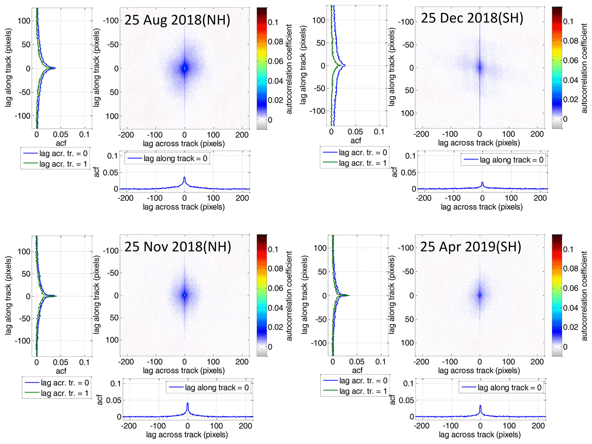
Figure 2Left: mean autocorrelation coefficients of orbital slices with across-track scans taken at SZAs between 60 and 75∘ for days without enhanced OClO as indicated in the respective colour plots. On the left and bottom of each colour plot the coefficients are plotted as line plots for the lag across track of 0 and 1 pixel and lag along track of 0, respectively. The values for both lags being zero are excluded (it is unity by definition). Note that the axis limits are selected to be in the same range as for the plots for the sensitivity studies with different retrieval parameters in Appendix B.
While at even larger lags the autocorrelation reaches zero in the across-track direction, it stays enhanced in the along-track direction and is distinctively larger when the across-track lag is 0. These distinctively larger values for the lags along track at the across-track lag of zero are caused by the detector striping effect. The correlation between nearby stripes at large lags along track is likely caused by structural patterns in the observed scene at the region where the earthshine reference has been obtained. According to Fig. 2, the correlation between nearby detectors seems to be smaller for 25 December in the SH, which could be caused by a less structured impact of the reference spectra across track than for other days as above ice the cloud effect plays a smaller role.
In summary, the contribution of local-scale systematic errors that can be detected by the autocorrelation analysis (the mean relation of one measurement to another in a statistical sense) is only a few percent; thus, it is not a dominating error source at the original instrument resolution. The investigation of autocorrelations, however, is still important, because for binned measurements (see next subsection), the local-scale systematic errors become important because of a lower variance of the gridded mean. Thus, the autocorrelation analysis provides an important contribution when evaluating the retrieval performance with different retrieval settings in the sensitivity studies in Appendix B.
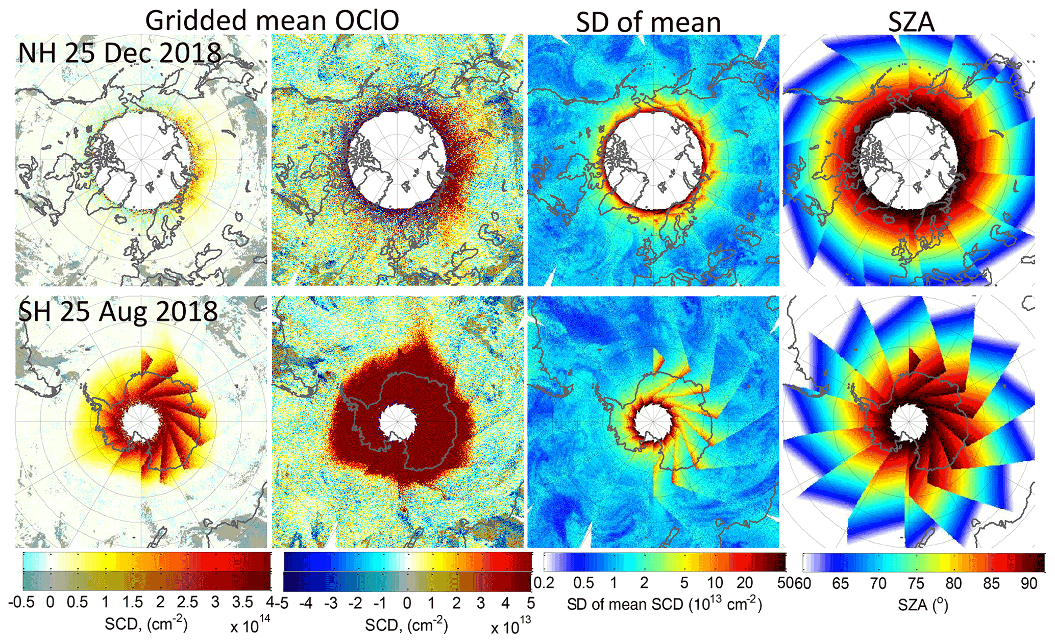
Figure 3Left plots: OClO SCDs for 25 December 2018 in the NH (top) and 25 August 2018 in the SH (bottom) binned on a grid in terms of an equidistant in latitude coordinate projection. Areas with cloud fraction (CF) below 5 % are shaded. Second column from left: same results but with a different colour scale. Second from right: standard deviation of the binned mean. Right: SZA of the plotted data.
2.2.3 Binning
Similarly as for the autocorrelation analysis, the large random errors (Fig. 1b), having the same magnitude as the OClO SCDs even for strong chlorine activation levels, make measurements hardly interpretable by eye at the TROPOMI resolution. Therefore, we apply a spatial binning. Figure 3 shows OClO SCDs for 25 December 2018 in the NH and 25 August 2018 in the SH binned on a grid in an equidistant in latitude coordinate projection (corresponding to an area of roughly 20×20 km2). Note that in the left columns the same results are shown but with colour scales either to illustrate the OClO SCD variation in the atmosphere or for the purpose of illustrating systematic features (compare Fig. 1). The figure also illustrates the standard deviation of the gridded mean (second column from right) and the SZA (right column). The gridded data show areas with increased OClO SCD values distinct from the very smooth background. This “real” OClO signal for the gridded data remains pronounced even for rather low OClO levels as for 25 December 2018 in the NH, because the standard deviation of the binned data is only around 5×1013 cm−2 at a SZA of 90∘. It is worth mentioning that a value of 5×1013 cm−2 is often referred to as a value for the OClO detection limit in the literature for GOME-1 and SCIAMACHY (Wagner et al., 2001; Oetjen et al., 2011). At lower SZAs the standard deviation of the mean decreases quickly by a factor of 10. This allows one to identify even localized systematic features whose existence was deduced from the spatial cross-correlation study in the autocorrelation study (see Sect. 2.2.2). They typically do not deviate from zero by more than cm−2 except for areas with very low cloud fraction (CF) where the deviation can be by a factor of 2 or 3 larger. Unfortunately, the performed sensitivity studies have not provided an explanation for this dependency. We could speculate that for clear sky cases the lower signal-to-noise ratio (due to a typically lower effective albedo), larger effects of the spectral stray light, imperfections in the detector linearity or the spectral polarization sensitivity of the instrument could play a larger role. To mark such cases, areas with CF below 5 % for SZAs below 75∘ are shaded in the figure.
Because OClO is highly variable, it is not possible to provide a general value for a typical relative error. Thus, we limit the error estimation to a few values for possible OClO SCD levels. The relative error of OClO SCD gridded data is about 15 % for a SCD of 5×1014 cm−2 at SZA of 90∘. This estimate is obtained by adding the squares of the relevant errors (cross section error 10 %, random error 5×1013 cm−2 and assuming the systematic error (offset magnitude) of 2×1013 cm−2). For a SCD of 2×1014 cm−2, this translates to an error of 30 %. For lower SZAs where both the expected levels of the retrieved OClO and the random error are substantially smaller, the relative error at a SZA 85∘ for an OClO SCD of 5×1013 cm−2 is estimated as 50 %.
The detection limit which we determine as the SCD value that corresponds to a relative error of 100 % is about 6×10¹³ and 2.5×1013 cm−2 at SZAs of 90 and 85∘, respectively.
2.2.4 Sensitivity to retrieval settings
To motivate the retrieval setup as introduced in Sect. 2.1, we investigated the effect of different retrieval settings on the retrieved OClO SCDs by applying modifications with respect to the standard fit scenario described in Sect. 2, Table 1. In Table 2 the specific settings for the sensitivity studies (second column) and corresponding main results (remaining columns on the right) are provided. We refer to Appendix B for a more detailed description of the obtained results. Table 2 summarizes the minimum and maximum offsets from zero (third column) for the same days introduced in Sect. 2.2.1 for which no OClO is expected (25 August 2018 for the NH and 25 December 2018 for the SH, 25 November 2018 (NH) and 25 April 2019 for SH) at SZAs of 90 and 85∘ for the modified settings (second column). The standard deviation of the binned mean (maximum from the investigated 4 d) is provided in the fourth column, while the autocorrelation coefficient for 25 November 2018 (NH) at lags of 1 and 20 pixels across track, both with a lag of 0 along track, are listed in the last column. Larger absolute values than for the standard case are marked in bold. Comparing these differences to the performance of the standard scenario, the case numbers of the settings (first column) are marked in bold, which are causing a worsening of the retrieval.
Kühl et al., 2004aOetjen et al., 2011(Beirle et al., 2017)Table 2Specific settings and results for the sensitivity studies; for details see Appendix B. Larger absolute values than for the standard case are marked in bold.
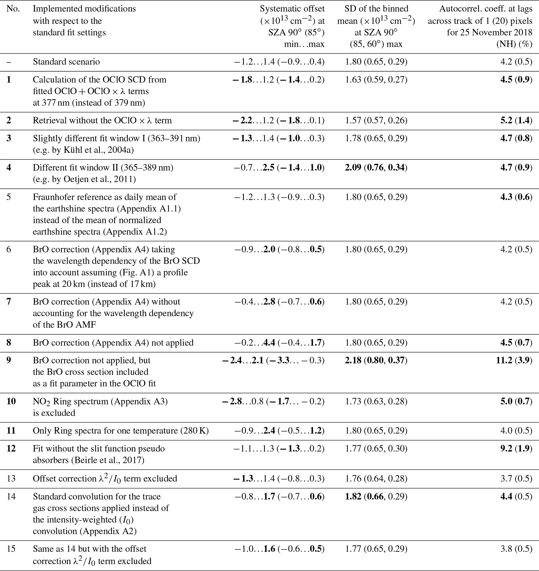
In particular, it is important to consider the OClO×λ term (compare to sensitivity case 2) and carefully select a wavelength for the calculation of the OClO SCD from the fitted terms (case 1), ensuring a minimization of the systematic error. The accuracy improvement here is larger than a slight increase in the random error. Also, special care should be taken when selecting the fit window (cases 3 and 4) where already small changes (case 3) can lead to a lower accuracy and increased background structures as clearly recognized by the autocorrelation analysis. For the retrieval of OClO, it is important to consider the BrO absorption. Adding a BrO cross section to the retrieval as a free fit parameter, however, leads to large retrieval errors (case 9). Applying a BrO correction (Appendix A4) by subtracting the BrO signal retrieved in another fit window suitable for retrieval of BrO is important to account for the wavelength dependency of the BrO air mass factor (AMF) (case 8). Interestingly, the exact BrO profile height, although providing a larger offset at higher SZAs, is not so important (case 7). Also the consideration of a NO2 Ring spectrum (Appendix A3) is providing a significant improvement. It is also necessary to include in Ring spectra calculated at two temperatures (case 11) as well pseudo absorbers accounting for changes in the slit function (Beirle et al., 2017).
Not important in the context of the investigated fit settings is the use of the (theoretically more accurate) mean of the normalized earthshine spectra (Appendix A1.2) instead of the mean of the earthshine spectra (case 5). Besides that, the offset correction term can also be neglected. Also the intensity-weighted convolution (case 14) is considered optional, leading to a correction of only about 3 times below the current accuracy level.
Although a nadir-viewing satellite instrument like TROPOMI and a ground-based zenith sky instrument are viewing in opposite directions (one downwards from space and another upwards from the Earth's surface), the absorption by OClO at high SZAs is taking place in the stratosphere, which, before the light is scattered into the instrument's field of view, is crossed by the light under the same slant angle for both instruments, i.e. is probing nearly the same air mass. Thus it is expected that also nearly the same photochemical variations along the light path take place. We compare OClO SCDs retrieved from TROPOMI measurements with those obtained by ground-based zenith sky DOAS instruments at Kiruna (Gottschalk, 2013; Gu, 2019), Sweden (67.84∘ N, 20.41∘ E), and at Neumayer station (Frieß et al., 2005) in Antarctica (70.64∘ S, 8.26∘ W). For the comparison, the OClO SCDs retrieved for all TROPOMI pixels within 100 km radius around the ground stations are averaged. To filter for outliers, TROPOMI pixels with fit errors above 10×1014 cm−2 are excluded. Also cases with less than 100 TROPOMI pixels within that area are excluded from further processing. For the zenith sky instruments, SCDs within the SZA range of around TROPOMI SZA are averaged.
3.1 Kiruna
The zenith sky DOAS instrument at Kiruna measures scattered sunlight between 300 and 400 nm with a spectral resolution of about 0.6 nm and approximately 10 times finer wavelength sampling. OClO SCDs from Kiruna used for this comparison are retrieved in a fit window of 372–392 nm. Cross sections for OClO (Kromminga et al., 2003) at 213 K, ozone (Bogumil et al., 2003) at 223 K, O4 (Thalman and Volkamer, 2013) at 273 K and NO2 (Vandaele et al., 1998) at 220 K are used. The intensity offset is considered by and terms. Also four Ring spectra (at temperatures of 213 and 263 K, scaled and not scaled with λ4) and a λ⋅σOClO term (Puķīte and Wagner, 2016) are included in the fit. As a Fraunhofer reference, an OClO-free spectrum, obtained before the winter in October at about 80∘ SZA at a day when Kiruna was outside the polar vortex, is taken.
The time series comparing both datasets are shown in Fig. 4 where the collocated TROPOMI measurements are indicated as circles and zenith sky measurements as crosses. Both are coloured according to the SZA. The circle radius also scales with the available TROPOMI pixel numbers within the collocated area, ranging from 100 to ∼1500. Figure 5 shows the difference between both datasets. Generally very good agreement can be found, not exceeding cm−2 for SZA at and below 90∘. Larger discrepancies (mostly within cm−2) appear at very high SZAs, where the scatter can be larger especially for comparisons with a low number of averaged TROPOMI pixels. This can also be seen in Fig. 6 where on the left-hand side the difference is plotted between the collocated TROPOMI and zenith sky DOAS measurements as a function of the SZA (x axis). The time of the measurement is provided by the colour scale. For SZAs below 90∘, a systematic offset of about 1×1013 cm−2 is found with a standard deviation that does not exceed this offset value. Close to the SZA of 90∘, the mean offset crosses zero and becomes negative at larger SZAs with standard deviation of about 4×1013 cm−2. Figure 6b shows a scatter plot between the TROPOMI and zenith sky data. The data are again coloured with respect to the SZA and the collocated TROPOMI pixel numbers. The plot includes two regression lines: a linear regression and an orthogonal regression with the latter being reported to be more adequate for independent datasets (Cantrell, 2008). Both regression results indicate good agreement. Nevertheless, the slope for the orthogonal regression (0.94) is much closer to unity than for the linear regression (0.85). The offset parameters are 1.0×10¹³ and 6.2×1012 cm−2, respectively. The correlation coefficient between both datasets is 0.94.
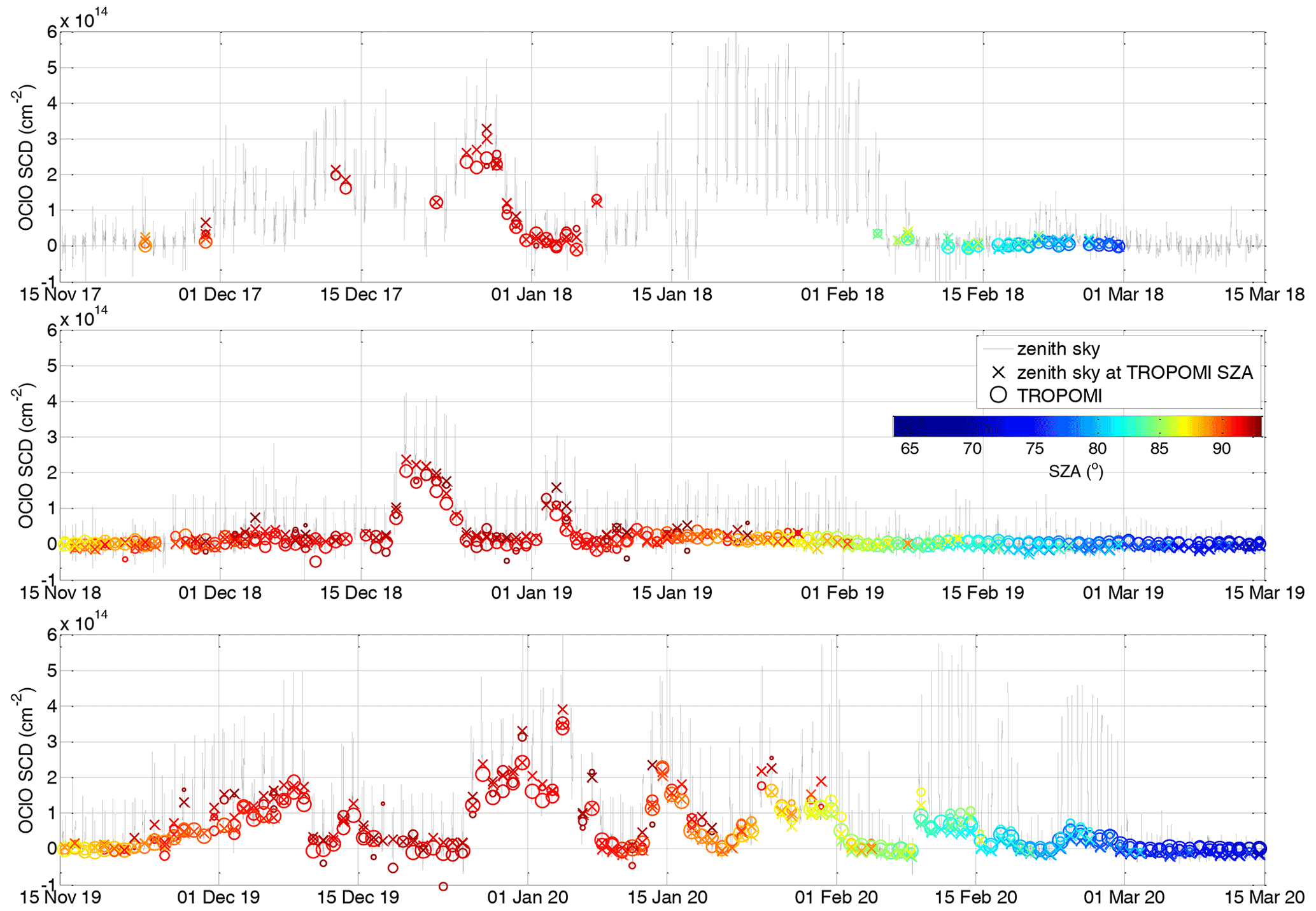
Figure 4OClO SCDs measured at Kiruna (67.84∘ N, 20.41∘ E) by the zenith sky DOAS instrument (black line). Their diurnal variation reflects their dependency in particular on SZA. The zenith sky measurements at the TROPOMI SZAs are marked by “×”. Collocated TROPOMI measurements are indicated by “o”. The SZAs of these measurements are colour-coded, while the radius of the circles indicates with the number of TROPOMI pixels within the selected area (in range of 100 to ∼1500).
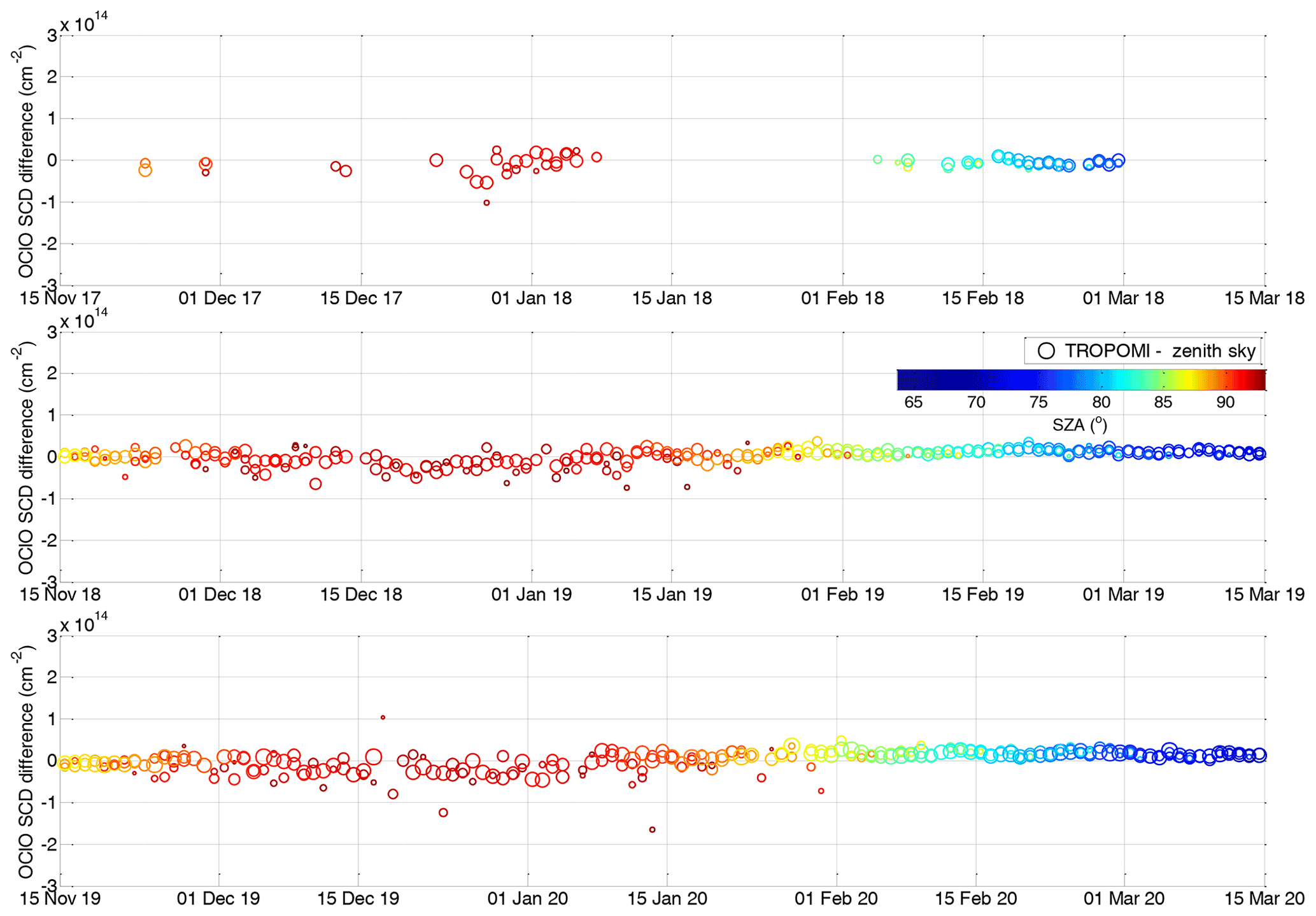
Figure 5Difference between the collocated TROPOMI OClO SCD measurements and the ground-based measurements in Kiruna for three different winters. Colour coding and radius of the circles is the same as in Fig. 4.

Figure 6(a) Difference between the collocated TROPOMI measurements and zenith sky DOAS measurements as a function of SZA (x axis) and the time of the measurement (colour scale). The mean and standard deviation of the data binned in a 1∘ SZA grid are indicated by the solid and dashed black lines, respectively. (b) Correlation plot between the TROPOMI and zenith sky measurements. The SZAs of these measurements are colour-coded, while the radius of the circles indicates the number of TROPOMI pixels within the collocated area. Orthogonal and linear regression lines between both datasets and their equations are provided in the legend.
It is also worth mentioning that the additional Ring spectra and the λ⋅σOClO term in the retrieval of Kiruna OClO SCDs improved the comparison with the satellite measurement dataset considerably. In Appendix C the comparison as in this subsection is presented but with Ring terms at only one temperature and without the λ⋅σOClO term. Also other settings for the retrieval of Kiruna OClO SCDs like the usage of a reference spectrum from a different day can slightly modify the offset. Nevertheless, the offset is below the accuracy of the retrieval and thus can be neglected.
3.2 Neumayer
The UV channel of the MAX-DOAS instrument at Neumayer station in Antarctica (Ferlemann et al., 2000; Frieß et al., 2001, 2005) measures scattered sunlight between 320 and 420 nm with a spectral resolution of 0.5 nm (full width at half maximum) by a 1024-element photodiode array. Note that for the OClO analysis only the zenith measurements are used. OClO SCDs for Neumayer are retrieved in the wavelength range of 364–391 nm. The fit settings include a fourth-order polynomial, cross sections for OClO (Kromminga et al., 2003) at 213 K, ozone (Bogumil et al., 2003) at 223 and 293 K, NO2 (Vandaele et al., 1998) at 220 and 298 K, O4 (Hermans, 2021) at 298 K, and BrO (Wilmouth et al., 1999) at 228 K. Also two Ring spectra (scaled and not scaled with λ4) and intensity offset ( term) are fitted. For the Fraunhofer reference, spectra in sunlit atmosphere outside the polar vortex are recorded.
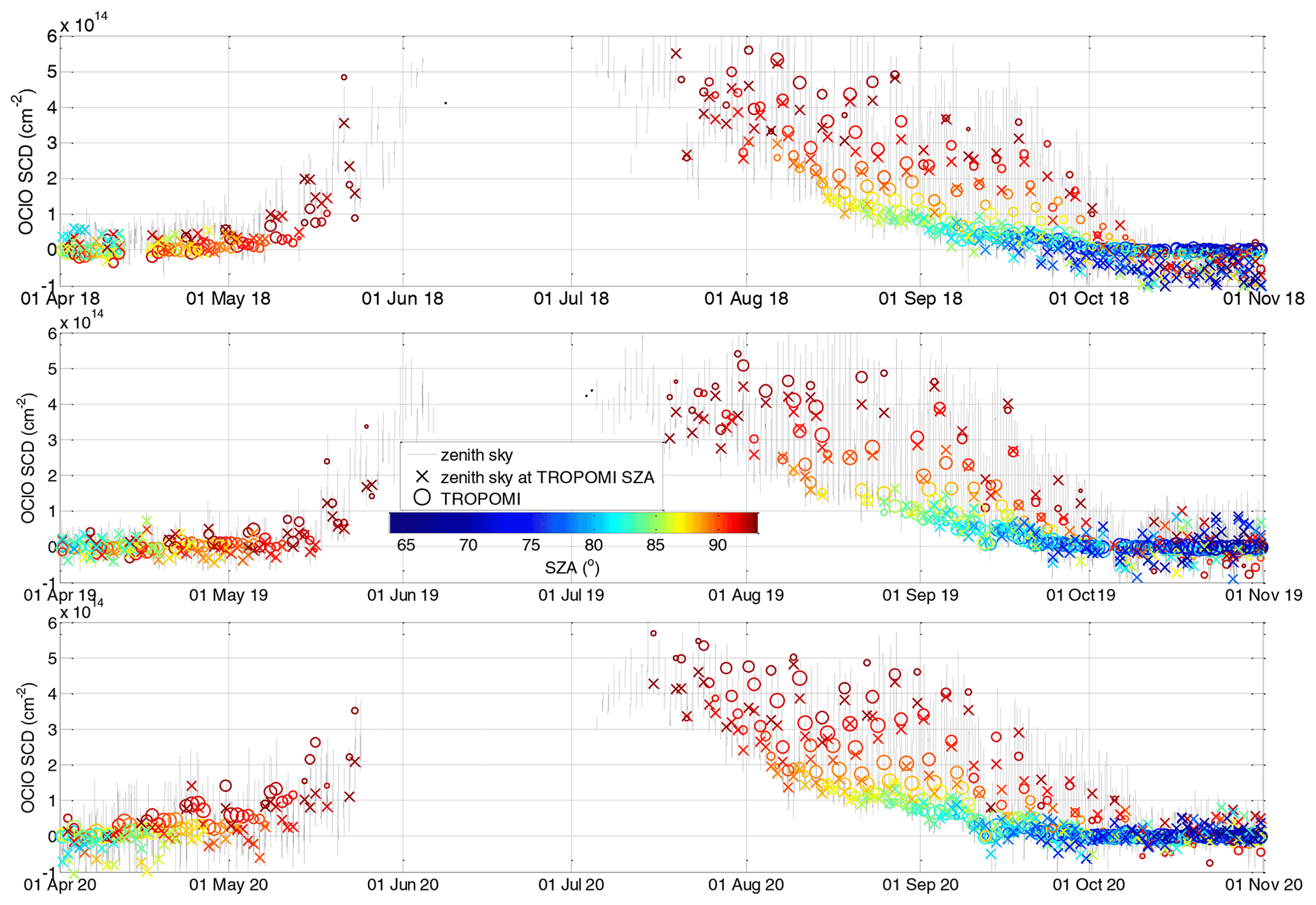
Figure 7Same as Fig. 4 but for zenith sky OClO SCDs measured at Neumayer (70.64∘ S, 8.26∘ W).
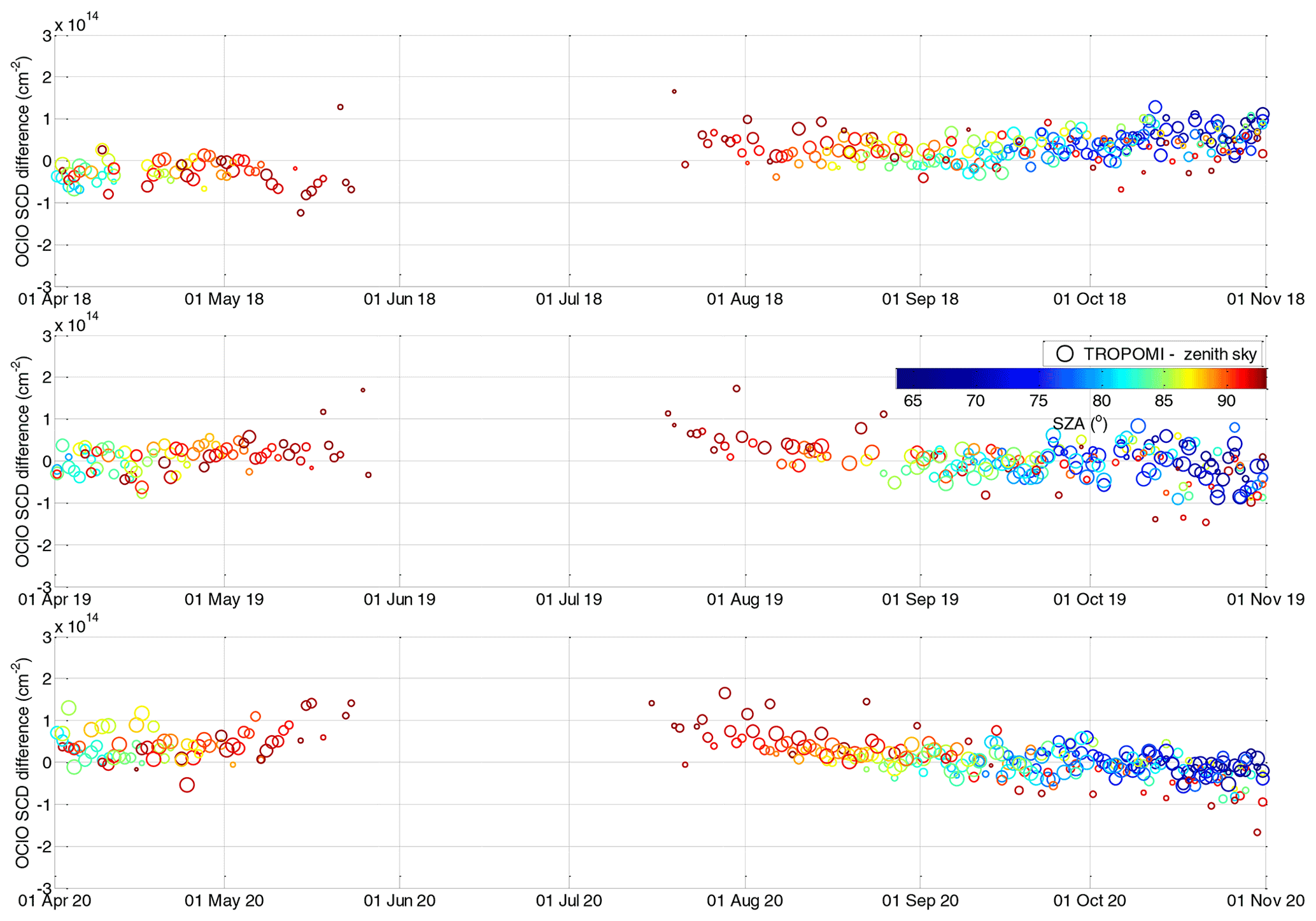
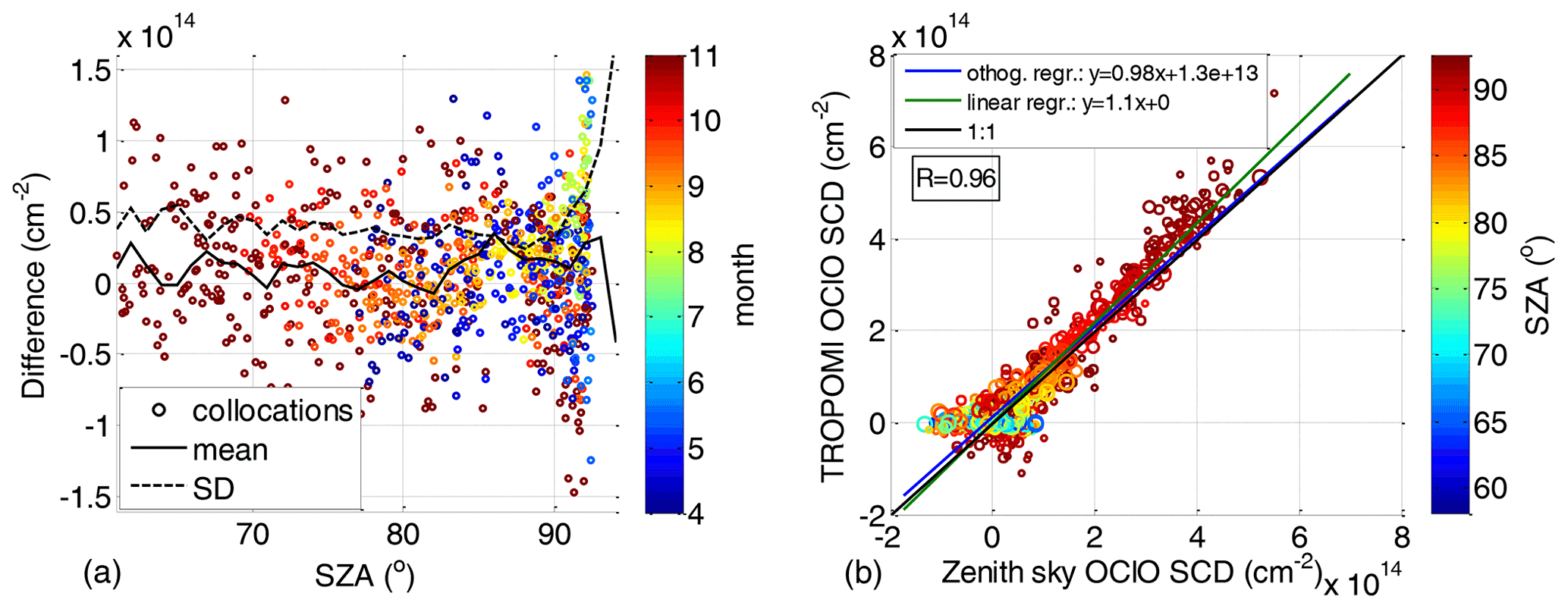
Figure 9Same as Fig. 6 but with zenith sky OClO SCDs measured at Neumayer (70.64∘ S, 8.26∘ W).
The time series shown in Fig. 7 are similar to those shown in Fig. 4 for the Kiruna measurements. Also the differences are provided in the same way as in Fig. 8. Also for the Neumayer data, good agreement is observed. The differences in most cases do not exceed cm−2 for SZA at and below 90∘ with a seasonal drift from local autumn until spring in the range of cm−2. The drift varies from year to year. For the polar winter 2018, the differences range from being mostly negative in April and May to mostly positive in September and October. For the winter 2019, the differences are scattered around zero both at the beginning and end of the season. However, an opposite trend is found for the winter 2020: the differences are mostly positive in April and May and become more negative in October. For all winters, mostly positive differences are observed at the end of July and beginning of August. This can also be seen in the left plot in Fig. 9 where the difference between the collocated TROPOMI and zenith sky DOAS measurements is plotted as a function of the SZA (with the time of the measurements indicated by the colour scale). At low SZAs which appear in April and also in September and November, the mean difference is in the range between 0 and 3×1013 cm−2, where the scatter reflects both the day-to-day variability and the differences between the different winters. The offset in July and beginning of August causes increased mean differences at a level of 2×10¹³ and 4×1013 cm−2 for SZAs above 87∘. At SZAs above 90∘ the scatter increases and also the differences between measurements in May and end of July–August show a different offset. The standard deviation of the differences is rather constant with SZA being around 4–5×1013 cm−2 for SZAs around 90∘ and below. We can speculate that the scatter for Neumayer in comparison with Kiruna is larger because of the different latitudes of both sites and the specific TROPOMI orbital properties along with the different retrieval settings. Figure 9b shows a scatter plot between the TROPOMI and zenith sky data. The linear regression provides slope parameter of 1.1, while for the orthogonal regression it is 0.98; the offsets are 0 and 1.3×1013 cm−2, respectively. The correlation coefficient (0.96) between both datasets is very similar to that for Kiruna (0.94).
In the framework of the Sentinel-5P Innovation activity (S5P+I) an operational OClO product from TROPOMI is under development. The current state of the algorithm (v0.95) is described in the Algorithm Theoretical Basis Document (Meier et al., 2020) in detail. Here just the basic settings are listed. The retrieval applies a solar irradiance spectrum as Fraunhofer reference and uses a fit window of 345–389 nm. Cross sections of OClO (Kromminga et al., 2003) at 213 K, NO2 (Vandaele et al., 1998) at 220 K, ozone (Serdyuchenko et al., 2014) at 223 and 243 K, O4 (Thalman and Volkamer, 2013) at 293 K, and Ring (Vountas et al., 1998) and intensity offset () terms. Also two empirical terms derived from mean residuals are used to account for contributions not explained by the already considered fit parameters.
We compare the retrieved OClO from our study with the preliminary S5P+I OClO SCD mean data within the range.
Figure 10 plots the time series of the S5P+I OClO SCDs together with those from this study for the polar winters 2018/19 and 2019/20 in the NH and 2018, 2019, and 2020 in the SH. While the overall shape agrees very well, an offset between both datasets is observed for low OClO levels where the S5P+I data have higher values. As discussed in Puķīte et al. (2021), OClO is not expected at the beginning of November (NH) or April (SH) because of still warm temperatures. Thus, values systematically above zero should likely be an artefact. At very high OClO levels the agreement becomes better. This behaviour is confirmed in the correlation plots in Fig. 11. A very high correlation is obtained with the correlation coefficient being 0.990 in the NH and 0.996 in the SH. The orthogonal regression has an offset of and cm−2, and the slopes are 1.10 and 1.07, respectively.
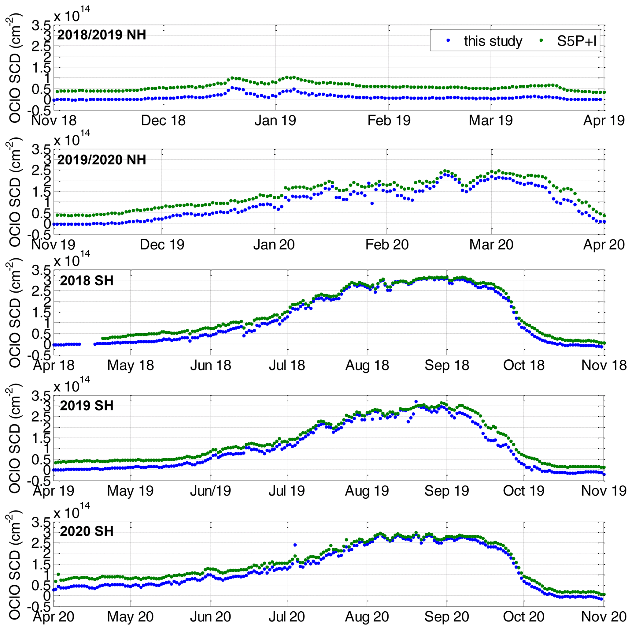
Figure 10Time series of TROPOMI mean OClO SCDs within obtained within this study and the preliminary data from the operational S5P+I data for polar winters (from top to bottom) 2018/19 and 2019/20 in the NH and 2018, 2019, and 2020 in the SH.

Figure 11Correlation plots between the time series shown in Fig. 10; left panel is for the NH winters and right panel is for the SH winters.
The slope is likely caused by the wavelength dependency of the OClO SCDs: for the interpretation we assume the same Gaussian profile shape as for BrO for the simulations in Fig. A1. The obtained ratio at the SZA of 90∘ between SCDs simulated at 380 and 340 nm is 1.35–1.9 (depending on profile peak altitude). Keeping in mind that the OClO SCDs for our study are obtained at 379 nm and assuming that the effective wavelength for the S5P+I is in the middle of their fit window (i.e. at 367 nm), we obtain a ratio in the range of 1.085–1.17 (broadly consistent with the observed slope). The slope different from unity and the offset of the regression thus explain the good agreement at high OClO SCDs and the offset at low SCD values.
A comparison of S5P+I OClO SCDs with the ground-based data (not shown here), performed in the same manner as the comparison in Sect. 3 between this study and the ground-based data, showed generally a very similar agreement between S5P+I and the ground-based data. Larger differences between the S5P+I OClO SCDs and the ground-based data than for our analysis was found for observations at high SZAs with low OClO SCDs, thus consistent with the findings in this section. As a consequence, the application of the solar irradiance instead of the earthshine spectrum as Fraunhofer reference cannot likely explain the differences as it would provide a similar offset for all SZAs. Also the use of a Ring spectrum as defined in the S5P+I preliminary product (not shown here) did not provide a better result. Thus we can speculate that the differences could be related to the usage of different fit windows, together with still uncompensated higher-order effects in the current version of the S5P+I OClO fit as the consideration of the wavelength dependency of fit parameters becomes more challenging in larger fit windows. The differences might also be related to the implementation of the empirical terms in the S5P+I retrieval or instrumental effects, but such investigations are beyond the scope of this study.
We developed a novel retrieval algorithm of OClO SCDs from the TROPOMI instrument on Sentinel-5P. To achieve the challenging high accuracy (and low detection limit), which is especially important for OClO observations, accounting for absorber and pseudo absorber structures in optical depth even of the order of 10−4 is important. Therefore, in comparison to existing retrievals, we include several additional fit parameters accounting for spectral effects like the temperature dependency of the Ring effect and Ring absorption effects. The analysis also considers higher-order terms (Puķīte and Wagner, 2016) and the BrO absorption contribution. Including these terms improves the accuracy of the retrieval results especially for low OClO SCDs. The typical random error is around 4×1013 cm−2 at low SZA (60∘) and reaches cm−2 at an SZA of 90∘. Thus for the interpretation of the data, averaging of individual measurements is needed to decrease the random error towards the typical levels of OClO SCDs. In this study we average the individual measurements on a horizontal grid of about 20×20 km2 (averaging about 20–25 individual measurements), which is well suited for measurements in the stratosphere.
For the gridded OClO SCDs, the random uncertainty is typically 0.5–1×1013 cm−2 at low SZA and 5×1013 cm−2 at SZAs around 90∘. Also, the systematic errors in this range are mostly not exceeding 1–2 ×1013 cm−2. Thus a detection limit of about 0.5–1×1014 cm−2 at a SZA of 90∘, similar to the detection limits of earlier instruments, is achieved but at a substantially lower spatial resolution. Thus TROPOMI OClO measurements provide a clear improvement with respect to previous instruments.
We investigated the performance of different retrieval settings by an error analysis with respect to random variations, large-scale systematic variations as a function of SZA and also more localized systematic variations by a novel application of an autocorrelation analysis.
The retrieved dataset agrees very well with zenith sky measurements in both polar regions (at Kiruna and Neumayer station) with slopes and correlation coefficients near unity. The larger absolute differences between individual TROPOMI and Neumayer data points are compensated by much higher absolute OClO SCDs at Neumayer. The use of similar settings for the spectral analysis for the Kiruna zenith sky measurements as those used for the TROPOMI analysis with an optimized treatment of the temperature dependency of the Ring effect and with an OClO cross section “lambda term” significantly improved the agreement, practically removing the year-to-year and seasonal variability in the difference between the TROPOMI and zenith sky datasets.
A nearly perfect correlation (correlation coefficient being practically unity) is obtained with the comparison to the preliminary data of the operational S5P+I retrieval algorithm. In the S5P+I data, however, a systematic positive offset with respect to the presented algorithm is found. Here we can only speculate that this offset might be caused by higher-order effects, which are probably more important in the larger fit window of the S5P+I retrieval. A slope slightly different from unity can largely be explained by the differences in the wavelength regions used for the DOAS fit in both analyses.
A1 Calculation of the earthshine reference spectra
A1.1 Mean earthshine reference
When an earthshine reference is used for the DOAS analysis, the measurements in a selected reference region are averaged, obtaining a mean radiance reference spectrum Iref(λ) as follows:
where indicates the individual measured spectra with τi(λ) being the signal of absorption features from a single pixel i to be contributing to absorption parameters fitted by the retrieval and the intensity Ii(λ) being the intensity of the signal; for example, for pixels above the clouds there will be a stronger signal than for clear scenes.
In DOAS, the logarithm of Eq. (A1) is used for the normalization of individual measurements. Expanding it in a Taylor series up to the first order with respect to τi(λ), one obtains the following:
The second term on the right-hand side indicates that the features τi(λ) in the mean earthshine reference spectrum are weighted with the intensities of the contributing measurements. Thus, such a reference spectrum in the DOAS analysis generally would lead to an offset for the fitted parameters even in the reference region if their SCDs are not homogeneous in this region. Also if there is no expected absorption of a particular absorber in the reference region (like it is the case for OClO), the potential errors and the incompleteness of the representation of the atmospheric state by the DOAS model can in theory induce an offset as part of the signal could interfere with the absorption cross sections of the considered absorbers. Fortunately the performed sensitivity studies (Appendix B5) show no additional effect from these considerations to the retrieved OClO SCDs. Nevertheless, we eliminate even a theoretical possibility of such an offset by considerations in the next subsection.
A1.2 Weighted mean earthshine reference with inverse radiance weights
To avoid this problem we normalize the individual measurements in the reference region before averaging:
Intensity Ii(λ′) is selected at a distinct wavelength λ′ within measurement spectrum Ii(λ).
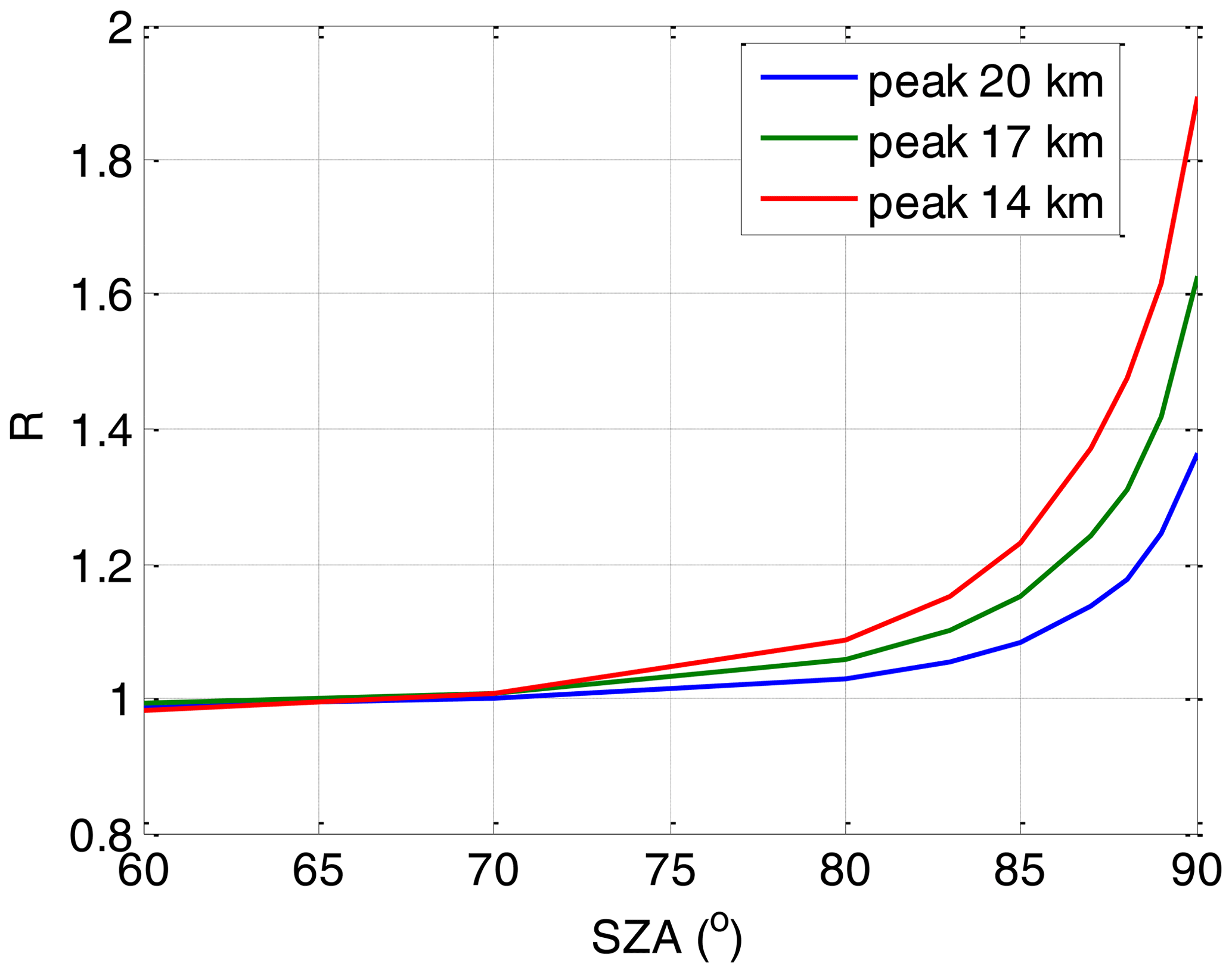
Figure A1Scaling factors R accounting for the BrO SCD differences at different wavelengths as a function of the SZA. For the BrO correction in the OClO retrieval, the factors modelled for a BrO profile with a peak at 17 km are used. Plotted also are values for two additional BrO profile peak altitudes.
Expanding the logarithm of Eq. (A3) in a Taylor series up to the first order with respect to τi(λ), one obtains the following:
Since is nearly proportional to all intensities in the spectrum Ii, there is practically no effective weighting for τi in the second term on the right-hand side. Thus, using a weighted spectrum (Eq. A3) as a Fraunhofer reference spectrum in the DOAS analysis at practically no additional calculation effort should eliminate even a theoretical possibility to an offset in the mean values of the fitted parameters in the reference region.
A2 Intensity-weighted convolution of cross sections
The so-called I0 correction is applied to account for the so-called absorption filling-in effect when convoluting absorber cross sections to the instrument resolution in DOAS applications (Wagner et al., 2002a; Aliwell et al., 2002). An I0-corrected cross section σLR for the low-resolution (LR) domain is calculated as follows:
where I0(λ) is the high-resolution (HR) Sun spectrum, K is the convolution kernel (i.e. ISRF) and S is the SCD. The result of the equation is twofold: first, it weights the absorptions at the individual wavelengths with the intensities of I0, and second, it considers non-linear effects of absorptions in the exponent. It follows that the equation, however, is valid for a single absorber. In such a case the optical depth of the absorption is solely due to this one absorber and can be described in the LR domain by the logarithmic ratio of the convolved spectra with absorption and without absorption:
The effective cross section in the LR domain is just the ratio of τLR and S, the last term is assumed to be constant and as such can be retrieved by the fit.
The problem is to deal with a situation when the assumption of a single absorber is not fulfilled, in particular if there is more than one absorber in the scene or the SCD varies with wavelength. In such a case the absorption optical depth is
Now the absorption optical depth cannot be normalized by a constant SCD of a single absorber. Moreover the absorptions Si(λ)σHR,i(λ) of the individual trace gases i have multiplicative effects; thus, in principle they cannot be convoluted separately, and their LR optical depths cannot be separated as would be needed for a correct definition of distinct LR cross sections.
A2.1 Weak absorption formalism
Assuming that the absorption is weak enough, a Taylor series expansion can be applied (i.e. for x close to 0); we can, however, state the following:
Now the summands can be integrated separately. Assuming also that the SCDs are constant, the I0-corrected cross sections for a weak absorption limit can be defined:
In cases where it is necessary to account for the SCD variation with wavelength, Si can be expanded in a Taylor series with respect to the wavelength and the cross section (Puķīte et al., 2010; Puķīte and Wagner, 2016):
Putting this expression into Eq. (A8), one just needs to also convolve in addition to Eq. (A9) the products of λσHR,i(λ) and σHR,i(λ)2 in order to obtain the I0-corrected cross sections for these higher-order terms:
By this intensity-weighted convolution of the cross sections, the first aim of the I0 correction (weights the absorptions at individual wavelengths with the intensities of I0) is fulfilled. For the application to the OClO SCD retrieval in this study, the intensity-weighted convolution (i.e. Eq. A9) is applied for all trace gas cross sections. The cross section wavelength term (Eq. A11) is used for the λ⋅σOClO term. Because of the weak absorption, the cross section square term (Eq. A12) is not applied.
A2.2 Strong absorption assumption
Although being not relevant for the OClO SCD retrieval, we take for the sake of completeness a short excursion to also show that the second aim of the I0 correction (i.e. accounting for the non-linear contribution to the absorption filling effect) can be considered in a similar manner by just the intensity-weighted convolution of the higher-order terms.
For a case with a strong absorption when the usage of the Taylor series square term is needed and thus also an absorption non-linearity effect in the I0 correction can be expected, we just need to explore the higher-order Taylor series expansion terms for the exponent of Eq. (A7). Consequently, Eq. (A8) can be written in a general form:
where SgσHR,g describes the absorption contribution of a particular term g obtained by the Taylor series expansion (for the definition of the higher-order DOAS terms please refer to Puķīte and Wagner, 2016, in particular Sect. 3.3 therein).
The I0-corrected cross sections are then generally defined as (compare to Eq. A9)
These terms include both the cross section wavelength term (σλ)LR,i (Eq. A11) as well as the cross section square term (σ2)LR,i (Eq. A12). Thus, it can be assumed that the intensity-weighted convolution of the higher-order terms implicitly also accounts for the non-linearity of the I0 filling in.
A3 Ring effect on NO2 absorption
The Ring effect describes the so-called “filling in” of solar Fraunhofer lines (Grainger and Ring, 1962) for scattered light measurements caused by the fact that part of the light undergoes inelastic (Raman) scattering. It results in a highly structured spectral fingerprint with respect to the direct Sun spectrum (see Wagner et al., 2009). Although the DOAS retrieval with an earthshine spectrum as a Fraunhofer reference largely reduces the magnitude of the Ring effect, it still needs correction because of the different filling-in magnitudes between the measurement and the Fraunhofer reference.
In addition we found that it is necessary to account for the filling in of the NO2 absorption in order to eliminate a pronounced systematic negative bias in the retrieved OClO SCDs at high SZAs; see Appendix B8. The absorption filling in appears because a part of the absorption occurs before the Raman scattering event where light is crossing atmosphere at a different wavelength than after the scattering. This effect tends to reduce the differential trace gas absorption (smoothing effect) and seems to not be substantially reduced by the usage of the earthshine reference in our retrieval algorithm because of significant differences in light paths of the inelastically scattered light between the measurement and the Fraunhofer reference.
Fish and Jones (1995) have first demonstrated the importance of the absorption filling where they estimated the underestimation in the retrieved NO2 slant column from studies on simulated spectra. Van Roozendael et al. (2006) applied an iterative correction in the ozone SCD retrieval by scaling of the effective slant column. More recently, Lerot et al. (2014) developed a semiempirical formulation to calculate filling-in factors for their ozone retrieval, which, once multiplied to the elastically scattered radiances, correct them iteratively for the structures introduced by the inelastic scattering processes.
For our correction we just use the Taylor series expansion, as outlined below, of the Ring spectrum with respect to absorption up to the first order and include the obtained first-order Ring absorption term (for NO2) as a free fit parameter directly in the fit, thus having a benefit that neither a radiative transfer modelling nor an iteration scheme is needed.
The inelastic scattering contribution at the detector wavelength λ0 without absorption is defined as
where λ is the incident wavelengths of the light entering the atmosphere and undergoing Raman scattering to the measurement wavelength λ0; σRaman is the Raman line spectral cross section, obtained according to Bussemer (1993).
While this Raman scattered light travels through the atmosphere, absorption by trace gases also takes place:
Sb and Sa describe parts of an absorber SCD before and after a Raman scattering event, respectively. σabs is the cross section of the relevant absorber. We consider here that just one Raman scattering event for individually contributing photon paths takes place, and we assume that the contribution to the absorption filling in by light paths with more than a single Raman scattering event along one light path is negligible.
Elastically scattered contribution with absorption (assuming the same effective light path) is given as
The Ring spectrum (Bussemer, 1993; Wagner et al., 2009) is defined as the ratio between the inelastic and elastic terms:
After mathematical simplification of the expression, we obtain
Now the equation is linearized by expanding it in a Taylor series with respect to Sb:
The first term on the right-hand side is the classical Ring spectrum. The second term considers the Ring effect due to filling in of trace gas absorptions. As it can be seen, this filling in depends on both the absorption cross section and the intensity structures, the product of whose are convoluted with the Raman scattering cross section. In this way individual Ring absorption spectra for any relevant absorber can be calculated and considered in the fit. In our retrieval it appeared to be relevant to consider a Ring absorption spectrum just for NO2. Here Sb is the quantity obtained by the fit, the rest is the Ring absorption spectrum. It is worth mentioning that for our application the Ring absorption spectrum is originally calculated on a high-resolution grid; during the retrieval it is just convolved to the instrument resolution by applying I0-weighted interpolation (Sect. A2). It is of course possible to also calculate it directly at the instrument resolution; however, this would mean its whole recalculation for each calibration.
A4 BrO absorption correction
Within the OClO fit window used in this study, weak BrO absorption structures also occur (Wahner et al., 1988). For the retrieval without considering BrO, systematically enhanced OClO SCDs are retrieved for periods where the presence of OClO is not expected. Since BrO has a strong yearly cycle with a maximum in winter (Sinnhuber et al., 2002), it is important to eliminate possible interferences with the retrieved OClO SCDs as far as possible in order to not misinterpret the OClO data.
Within the chosen OClO fit window, the BrO cross section shows only very weak spectral features. Thus including the BrO cross section directly in the OClO fit as a free fit parameter leads to unreliable BrO results and accordingly in a systematic negative offset in the retrieved OClO SCDs. To overcome this problem, we use BrO SCDs, SBrO, provided by Warnach et al. (2019), retrieved in another fit window (330.6–352.75 nm) which is better suited for the BrO retrieval to subtract the BrO absorption from the measured spectra before performing the OClO DOAS fit.
The correction term
is subtracted from the left-hand term of Eq. (1). σBrO is the BrO cross section (Wahner et al., 1988) within the OClO fit range convolved with the ISRF. Since at high SZAs radiative transfer differences between different wavelengths can become important, a scaling factor R is used, defined as
where S380 and S340 are the BrO SCDs simulated by a radiative transfer model at the wavelengths of 380 and 340 nm, respectively. For R used in the retrieval, a BrO profile with peak at 17 km altitude and a Gaussian shape with FWHM (full width at half maximum) of 6 km is assumed. R of course is sensitive to these settings but it is better to apply this correction even with possibly inaccurate settings than not to apply it (see the sensitivity studies in Appendix B6). Figure A1 shows the dependency of R as a function of SZA for three different BrO peak heights showing the importance of this correction at high SZAs (scaling factor is 1.6 at SZA of 90∘). The uncertainty related to the peak altitude by 3 km is up to 0.3.
We investigate the effect of different retrieval settings on the retrieved OClO SCDs by applying modifications with respect to the standard fit scenario described in Sect. 2, Table 1. The considered cases with the corresponding changes are given in Table 2 in Sect. 2.2.4. The retrieval performance for the same days (25 August 2018 (NH) and 25 December 2018 (SH); 25 November 2018 (NH) and 25 April 2019 (SH); and 25 December 2018 (NH) and 25 August 2019 SH) as introduced in Sect. 2.2, Fig. 1, representative for different atmospheric conditions, is studied.
The obtained daily mean OClO SCDs for the defined cases are plotted in Fig. B1 for all 6 d. Since the standard deviations of the gridded means are very similar for the different months except 25 December in the SH (where the relative differences between the cases are still very similar as for the other days), an example for the standard deviation of the mean for just one of the days (25 December in the NH) is shown in Fig. B2. In addition, Fig. B3 displays the autocorrelation coefficients calculated as described in Sect. 2.2.2 as a function of the across-track lag for a zero along-track lag. The figure allows for a quantitative judgement about the magnitude of any systematic spatial artefact structures between the different retrieval settings. Figures B4 and B6 provide the retrieved binned OClO SCDs, and Figs. B5 and B7 provide their differences with respect to the standard scenario. These plots are shown for 25 November 2018 (NH) and also for 25 December 2018 (SH) in order to illustrate the seasonal differences. It is again found that the autocorrelation coefficients for 25 December 2018 (SH) are quite different from those of the other investigated days.
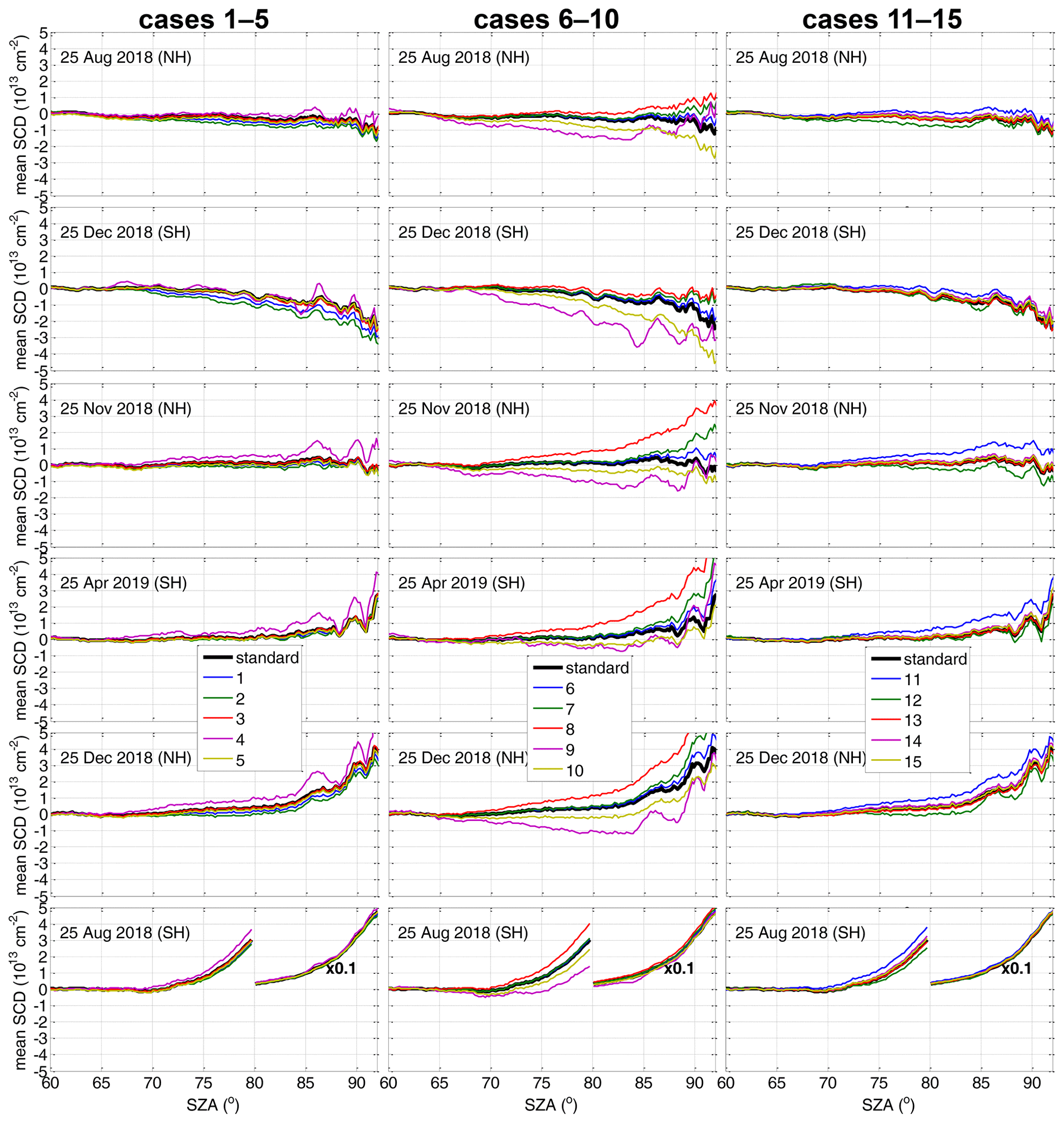
Figure B1Retrieved daily mean OClO SCDs as a function of SZA (resolution 0.2∘) for the different cases of the sensitivity study described in Table 2 in comparison to the standard scenario for selected days in both hemispheres.
In the following, we discuss the findings for the different cases.
B1 Case 1: wavelength assumption for the OClO×λ term
As suggested in Puķīte and Wagner (2016), when higher-order terms are applied in the fit, the wavelength for the calculation of the trace gas SCD from the fitted coefficients should be selected empirically from within the fit interval, because the agreement with the true SCD can vary with wavelength (as shown, for example, in the sensitivity studies for BrO in Puķīte et al., 2010). To demonstrate the effect of the wavelength selection for the retrieval of the OClO SCDs, we changed the recalculation wavelength to 377 nm instead of our standard wavelength of 379 nm. The retrieved OClO SCDs are reduced by up to 0.5×1013 cm−2 at large SZAs (blue line in the left plots in Fig. B1) compared to the standard setting for the summer days. The shape of the SZA binned mean SCD dependence, however, is very similar to that of the standard scenario. The standard deviation is even slightly better (blue line in Fig. B2, left panel), which is expected, because the wavelength is closer to the centre of the fit interval. This case, however, has an increased autocorrelation (see blue lines in left plots in Fig. B3), being especially strong for 25 December 2018 (SH) with more than 2 times higher values at the wings of the function. It shows an autocorrelation of 5 ‰ even at a lag distance across track of 70 pixels, while the value for the standard scenario is close to zero already for much shorter lags. Also for the 25 November 2018, the autocorrelation is much larger than for the other fit scenarios and is still above zero at large lags. The increase in the spatial structures can also be clearly seen in the maps of the binned OClO SCDs (Figs. B4–B7, upper row, left centre plot).
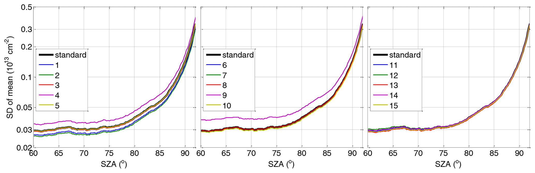
Figure B2Standard deviation of the binned mean OClO SCD for 25 December 2018 in the NH for the different cases of the sensitivity study described in Table 2 in comparison with the standard scenario for selected days in both hemispheres.
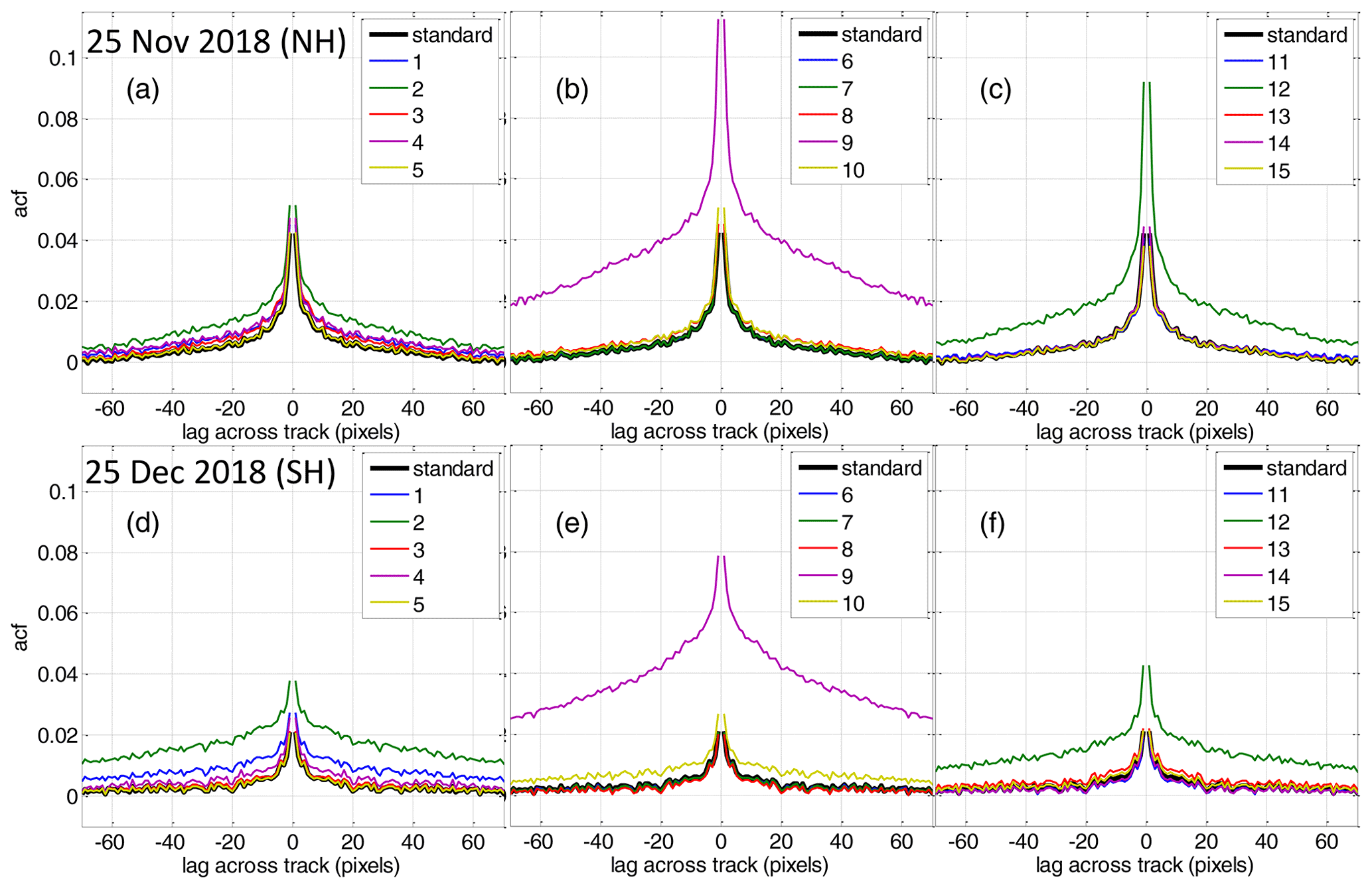
Figure B3Autocorrelation coefficients calculated as in Fig. 2 but for different cases of the sensitivity study as a function of lags across track with a lag along track of 0. Result for 25 November 2018 (NH) (a–c) and 25 December 2018 (SH) (d–f).
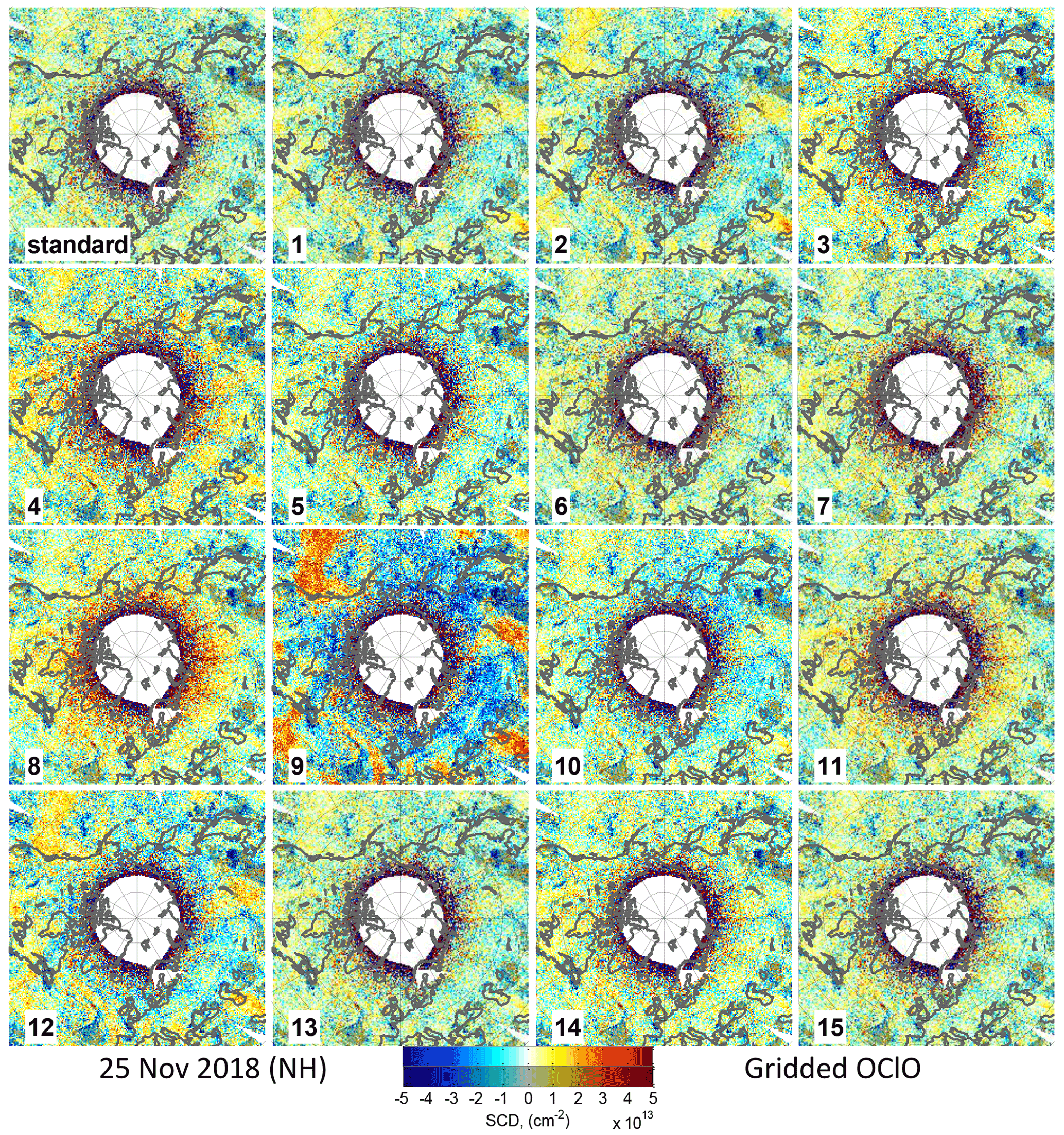
Figure B4OClO SCDs for 25 November 2018 in the NH binned on a grid in an equidistant in latitude coordinate projection. Areas with cloud fractions (CF) below 5 % are shaded.
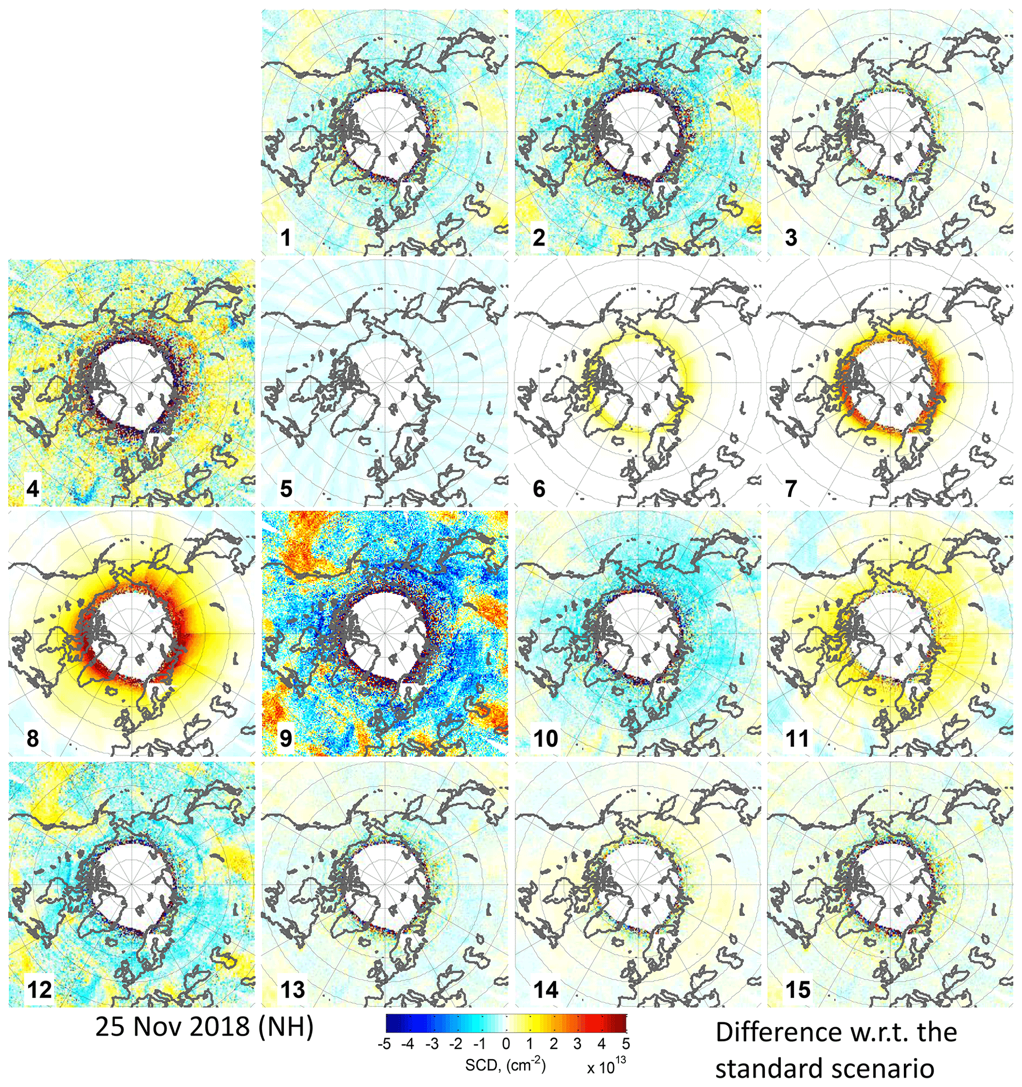
Figure B5Differences between the OClO SCDs shown in Fig. B4 and those of the standard scenario.
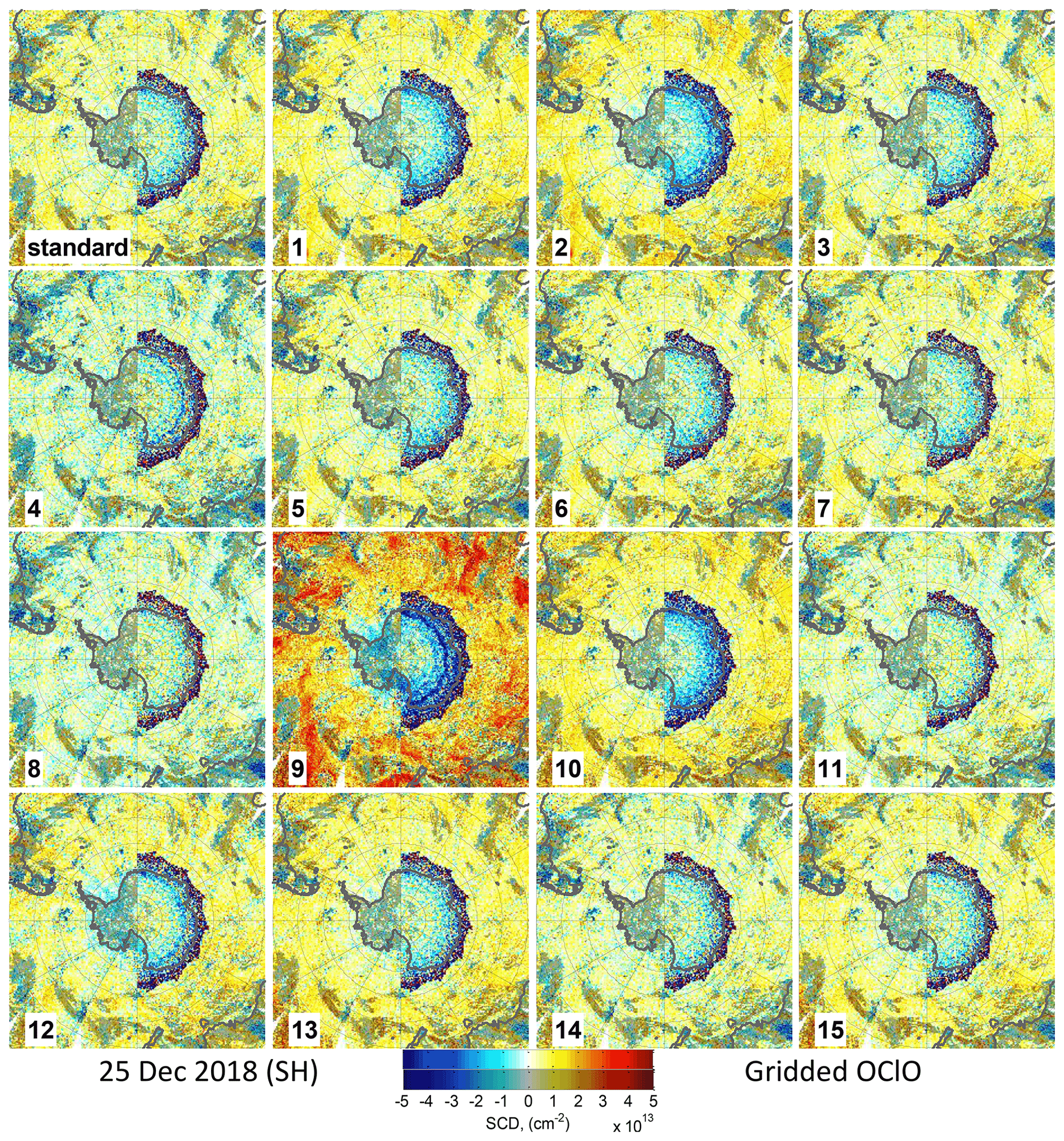
Figure B6Same as Fig. B4 but for 25 December 2018 in the SH. Note the different treatment with respect to the descending orbit parts (with higher SZAs): in the western hemisphere, only data for the ascending parts are shown, while in the eastern hemisphere data of the descending parts are plotted when available.
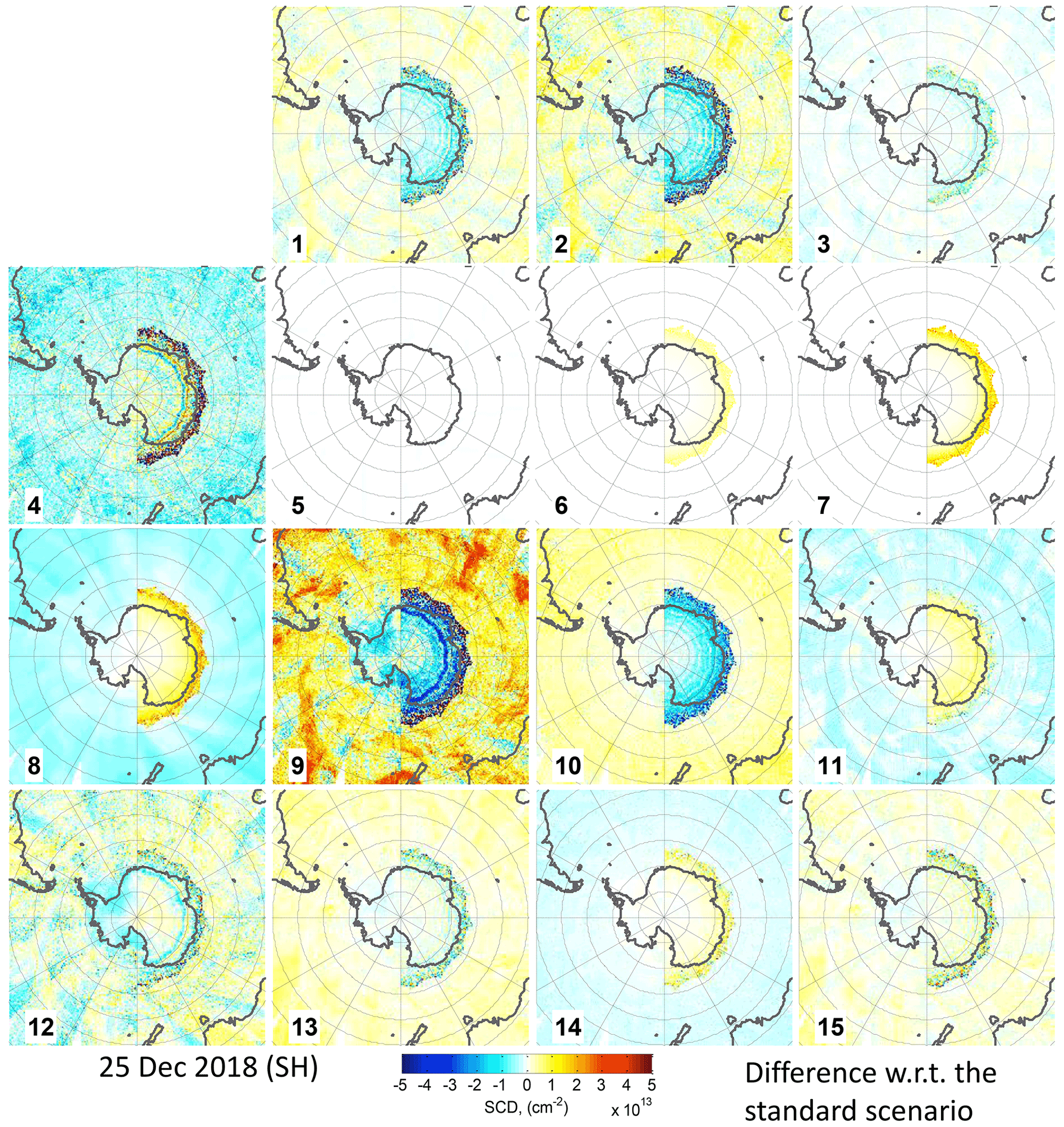
Figure B7Same as Fig. B5 but for 25 December 2018 in the SH.
This case shows that for the selection of the wavelength for the SCD calculation from the retrieved coefficients from the higher-order terms, a trade-off has to be found between precision and accuracy.
B2 Case 2: skipping OClO×λ term
In this case only the constant OClO cross section term is fitted, and the obtained SCDs are compared. In this case the retrieved SCDs are even (∼2 times) lower than for case 1, being again largest at high SZAs (up to 1×1013 cm−2, green line in the left plots in Fig. B1). The standard deviation (green line in Fig. B2) agrees quite well with that of case 1, indicating that adding higher-order terms does not reduce the random retrieval error per se. The autocorrelation (green line in the left plots in Fig. B3) for this scenario, however, is more than 4 times larger than for the standard scenario, indicating the appearance of even larger systematic spatial structures than for case 1. The binned OClO SCDs (Figs. B4–B7, upper row, right centre plot) confirm the increase in the systematic structures.
Thus we can conclude here that it can be beneficial to add the higher-order lambda term for the trace gas of interest to improve the performance of the retrieval with respect to systematic errors.
B3 Case 3: fit window 363–391 nm
The selection of the fit window used in our study (363–390.5 nm) is based on previous studies in our group (e.g. Kühl et al., 2004a). While on average the result for this scenario (red lines in the left plots in Figs. B1 and B2) agrees well with the result for the standard retrieval, the autocorrelation coefficients for this scenario (red line in left plots in Fig. B3) are somewhat larger in some cases like for 25 November 2018 (NH) where it is as large as for the case 1 for shorter lags. In the maps of binned OClO SCDs (Figs. B4–B7, upper row, right plot), small differences can also be seen.
B4 Case 4: fit window 365–389 nm
We also tested the fit window (365–389 nm) which has been used by Oetjen et al. (2011). Unfortunately, the use of this fit window gives much worse results which can be seen already in the plot with the gridded mean OClO SCDs as a function of SZA as a systematic “wavy” structure (magenta line in the left plots in Fig. B1). Interestingly, this structure has its peaks and depths at the same SZA values for all seasons and both hemispheres, possibly indicating some instrumental problem (we see similar structures in the results for different cases in general; only the amplitude is different). The interannual variation for this scenario is larger: in the autumn and winter months there is a large positive offset with respect to the standard scenario, while in summer this offset, still positive, is smaller. Interestingly, in summer the results of this scenario are closer to the expected value of zero than those of the standard analysis. This wavelength range selection, however, increases the random error (magenta line in Fig. B2). The autocorrelation is also increased (magenta line in the left plots in Fig. B3) compared to the standard scenario. But since the autocorrelation coefficients are calculated at lower SZAs, the large OClO variability at high SZAs does not show up here. However, the binned OClO SCD maps (Figs. B4–B7, middle upper row, left plot) show these wavy structures like rings at high SZAs.
B5 Case 5: Fraunhofer reference as daily mean of the earthshine spectra
In this setting, Fraunhofer reference spectra calculated as daily mean of the earthshine spectra (Appendix A1.1) instead of the mean of the normalized earthshine spectra (Appendix A1.2) are used for the retrieval. The dark yellow lines in the left plots in Figs. B1, B2 and B3 show perfect agreement with the standard scenario. The binned difference (second row, middle left plot in Fig. B5) shows only a very small detector striping.
B6 Cases 6–8: BrO correction
Cases 6–8 demonstrate the effect of the application of different aspects of the BrO correction (Appendix A4). In case 6, just the altitude of the profile for which the ratio of the BrO SCD between 380 and 340 nm (Fig. A1) are calculated is modified. The peak of the profile is assumed to be at 20 km instead of 17 km. In case 7, the wavelength dependency is ignored (i.e. the same SCD is assumed in both spectral ranges), while in case 8 BrO correction is not applied at all; i.e. the BrO absorption contribution is not subtracted from the measurement spectra.
The blue, green and red lines, middle column in Fig. B1, respectively, show the systematic effects of these settings. For all these cases, a positive offset with respect to the standard scenario is found, being larger for the days where more BrO is observed (in autumn and winter). When the BrO correction is not applied, artificially enhanced OClO SCDs of 3–4×1013 cm−2 (25 November in 2018 and 25 April 2019 in SH) at an SZA of 90∘ are retrieved. When applying the BrO correction but without considering the SCD dependency on wavelength, the offset is corrected up to SZAs of ∼85∘, because the BrO SCDs are almost independent of the profile shape and wavelength at short wavelengths. At a SZA of 90∘, the retrieved artificially enhanced OClO SCDs are, however, decreased by about a factor of 2 for the 2 autumn days. Thus, an offset at a level of cm−2 remains. This is further corrected by considering the BrO SCD wavelength dependency between the fit window of the BrO retrieval and the OClO fit window. Depending on whether the BrO profile at 17 km (as in the standard settings) or 20 km is chosen, the result varies by less than 1×1013 cm−2. The effect of the BrO correction for the days in summer where low BrO levels are expected is much smaller and is even leading (or contributing) to a negative offset of around 1×1013 cm−2. The BrO correction settings have no effect on the random error (B2, middle plot, where the respective blue, green and red lines overlap with the standard case). Also the autocorrelation coefficients (blue (overlaid by green), green and red (largely overlaid by yellow for the 25 November 2018) lines in the middle plots in Fig. B3) match (except for case 8 in autumn) the result for the standard case as the implemented settings have an effect for high SZAs (cases 6 and 7) or for large BrO SCDs (case 8 in the plot for 25 November 2018 in the NH). The binned OClO SCD maps (Figs. B4–B7, middle upper row, the two plots on the right-hand side for cases 6 and 7, and the middle lower row on the left-hand side) also indicate mostly latitude-driven (i.e. SZA) differences with respect to the standard scenario. Some additional variation also in east–west direction for case 8 (middle lower row, left plot in the same figures) caused by a larger stratospheric dynamics in BrO probably explains the slightly increased autocorrelation for the autumn day.
B7 Cases 9: BrO included as a fit parameter
It would be a more straightforward approach to use a BrO cross section directly in the OClO retrieval as additional fit parameter instead of the BrO correction described above. However, the results of this subsection illustrate that this is not a good choice: the retrieved OClO SCDs suffer from a strong offset exceeding the systematic uncertainties even at relatively low SZAs (Fig. B1, magenta line in the middle column), and it also shows the wavy structures as also seen in case 4. Also the random error is significantly larger than for most other settings (magenta line in middle plot in B2). The large systematic structures also show strong spatial variation as indicated by the results of the autocorrelation analysis (magenta line in the middle plots in Fig. B3) and in the binned OClO SCD maps (Figs. B4–B7, plots in the middle lower row, middle left).
B8 Case 10: skipping NO2 Ring absorption spectrum
In this case, the NO2 Ring absorption spectrum (Sect. A3) is excluded from the retrieval. As a consequence, a negative offset of up to around 2×1013 cm−2 with respect to the standard scenario is observed towards larger SZAs (Fig. B1, yellow line in the middle column). Also in the binned OClO SCD maps (Figs. B4–B7, plot right from and below the middle), a clear latitudinal gradient can be observed with respect to the standard scenario. As expected, this deviation is larger for the summer months where more stratospheric NO2 appears at higher latitudes than in the winter months. The random error is slightly smaller than for the standard scenario (dark yellow line in the middle plot in B2). The autocorrelation coefficients (dark yellow line in the middle plots in Fig. B3) are increased and are also larger in summer, obviously corresponding to the increased impact of the NO2 spatial distribution on the OClO retrieval.
B9 Case 11: Ring spectra at just one temperature (280 K)
The consideration of Ring spectra in the retrieval is one of the parameters we found, to which the retrieval settings are sensitive. Excluding the second Ring spectra for the temperature of 210 K from the retrieval (blue lines in the right plots in Fig. B1) also introduces a seasonally dependent offset (in this case being positive at larger SZAs) with respect to the standard scenario. Opposite to the results in case 10 (skipping the NO2 Ring spectrum), in this case the offset is larger for days in autumn and winter. There is practically no effect of this change on the random error (B2, right plot, blue line). Interestingly, also the autocorrelation coefficients (Fig. B3, right plots, blue line) are a bit larger than for the standard case. A potential explanation is that the spatial structures have a much coarser structure which is not well covered by the single orbit subsets used in the autocorrelation analysis. Also the binned OClO SCD maps (Figs. B4–B7, right plot, lower middle row) show differences in the systematic structures which besides the latitudinal variation also vary along longitude.
B10 Case 12: retrieval without slit function pseudo absorbers
The parameterization of slit function changes (Beirle et al., 2017) is also important for our retrieval: already in the SZA-resolved daily mean plots (green lines in the right plots in Fig. B1) a more pronounced fluctuation is found if this parameterization is not considered. The autocorrelation analysis (green lines in the right plots in Fig. B3) shows both much higher correlations for short as well as for long lags. This increase could be caused by the slit function variability, e.g. by the inhomogeneous illumination of the slit, the polarization sensitivity or other factors. The much larger spatial variation can also be seen in the binned OClO SCD maps (Figs. B4–B7, left plots in the bottom row). The setting of this case, however, has no effect on the random error (B2, right plot, green line).
B11 Case 13: offset correction term excluded
In our standard retrieval we consider an intensity offset correction up to the second order (i.e. the , and terms) There is a very small effect when the term is skipped (red lines in the right plots in Figs. B1–B3, and the middle left plots in the bottom row of Figs. B4–B7). Hoverer. it should also be noted that a larger discrepancy between the results of this case and the standard scenario is found in the autocorrelation coefficients for 25 December 2018 (SH). The fact that these orbital subsets are observed over Antarctica leads to larger measured radiances and thus might lead to a different stray-light contribution.
B12 Case 14: application of a standard convolution
In this case study, we apply a standard convolution for the trace gas cross sections instead of the intensity-weighted (I0) convolution described in Sect. A2. As observed in Fig. B1 (magenta lines, right plots) and the binned OClO SCD maps (middle right plots at the bottom row of Figs. B4–B7), this setting introduces a small but still distinguishable positive offset with respect to the standard scenario. This offset is larger in summer, indicating that it might mainly be caused by differences in the NO2 absorption cross section treatment whose absorption is larger in this season.
B13 Case 15: application of a standard convolution and an offset correction term excluded
During the sensitivity studies described above, we found that in some cases there can be a larger effect with respect to the offset correction term if the standard convolution is performed. Indeed, Fig. B1 (dark yellow lines, right plots) shows a better agreement of this case (when both standard convolution for trace gas cross sections are used, and the is omitted) with the results of the standard scenario than case 14. The results of case 15, however, have a higher autocorrelation (Fig. B3, right plots, dark yellow line) than those of the standard case.
In this appendix, we repeat the comparison between the zenith sky measurements at Kiruna and TROPOMI as in Sect. 3.1 but with the Kiruna OClO SCDs retrieved using just two Ring spectra (scaled and not scaled with λ4) at only one temperature (250 K) and without the OClO×λ term in the DOAS fit.
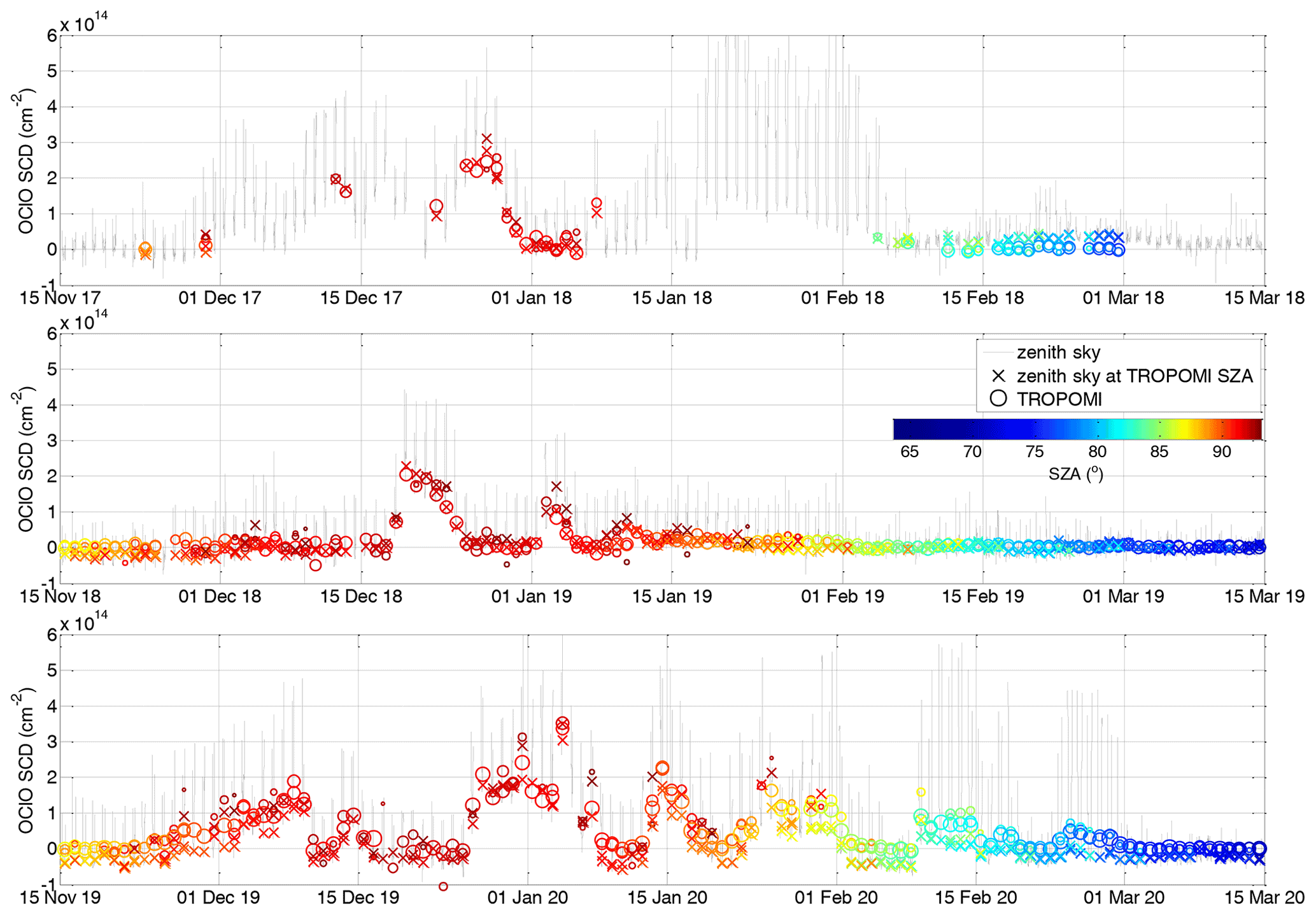
Figure C1Same as Fig. 4 but comparison with ground-based OClO SCDs at Kiruna retrieved with Ring spectra at a single temperature and without the OClO×λ term in the DOAS fit.
The timelines comparing both datasets and their difference are shown in Figs. C1 and C2 in the same manner as is done in Figs. 4 and 5 (Sect. 3.1), respectively. Along somehow larger absolute discrepancies (up to 8×1013 cm−2 for SZA at and below 90∘) than in Sect. 3.1, also pronounced inconsistencies are observed in a form of an offset between the TROPOMI and Kiruna SCDs being different for different winters. The difference between the datasets of both instruments also varies on a weekly or semi-monthly basis, inducing a wavy pattern in the difference plots. Also an overall trend can be recognized with an increasing difference increasing from the beginning of winter towards spring. Figure C3 illustrates the worsening of the comparison with respect to the agreement found in Sect. 3.1 (Fig. 6) even more clearly: a larger scatter in the difference between the collocated TROPOMI and zenith sky DOAS measurements as a function of the SZA (x axis) is visible in the left plot. The seasonal variability in the offset shows a clear dependency on SZA being at maximum as high as cm−2 (i.e. up to around 3 times larger than for the settings in Sect. 3.1) for SZAs between 85 and 90∘. Also the standard deviation of the differences is up to ∼3 times larger (for SZAs below and around 90∘). The scatter plot (Fig. C3a) between the TROPOMI and zenith sky data shows a worse correlation. The slope for the orthogonal regression is now only 0.75 (0.94 in Sect. 3.1), whereas the offset is 9.4×1012 cm−2 (1×1013 cm−2). The correlation coefficient between both datasets is 0.86 (0.94).
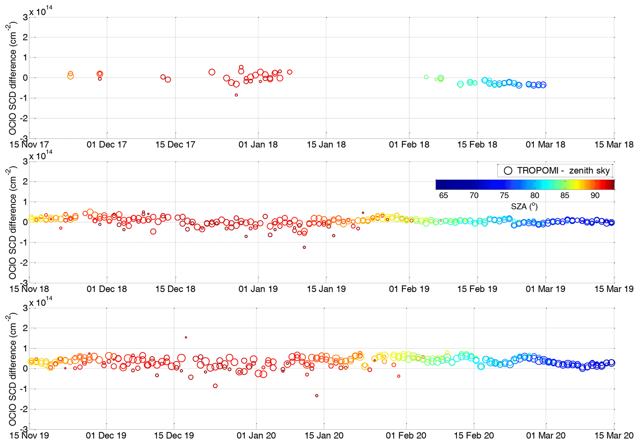
Figure C2Same as Fig. 5 but considering ground-based OClO SCDs at Kiruna retrieved with Ring spectra at a single temperature and without the OClO×λ term in the DOAS fit for the calculation of the difference.
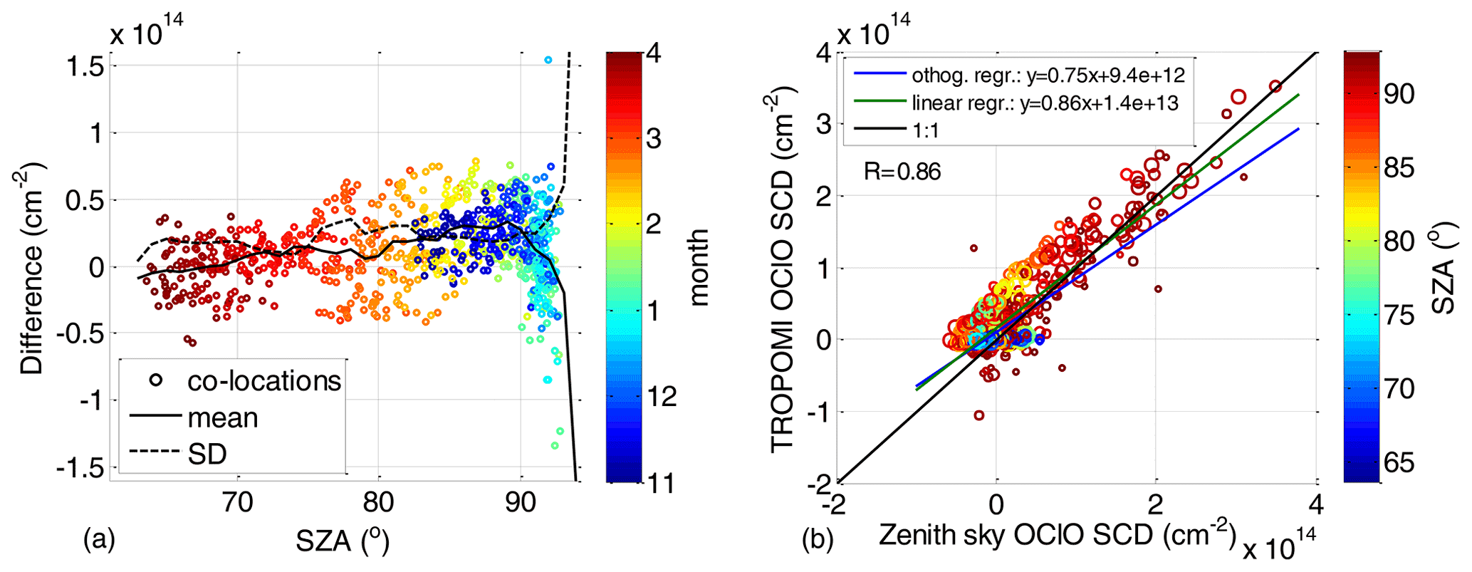
Data are available upon request from the corresponding author (janis.pukite@mpic.de).
JP with support of CB, SD, MG and TW performed the study and analysed the results. CB with support of JP and TW retrieved OClO SCDs from TROPOMI measurements. MG with support of JP and TW retrieved OClO SCDs from zenith sky measurements at Kiruna. UR and CFE maintained the zenith sky instrument at Kiruna. UF provided OClO SCDs from zenith sky measurements at Neumayer. AM and AR provided the preliminary S5P+I OClO SCDs. JP prepared the article with supervision by TW and comments by all co-authors.
The contact author has declared that neither they nor their co-authors have any competing interests.
Publisher's note: Copernicus Publications remains neutral with regard to jurisdictional claims in published maps and institutional affiliations.
We acknowledge the ESA and S5P teams for providing TROPOMI l1b data. We thank Simon Warnach for providing the TROPOMI BrO dataset.
The article processing charges for this open-access publication were covered by the Max Planck Society.
This paper was edited by Michel Van Roozendael and reviewed by three anonymous referees.
Aliwell, S. R., Van Roozendael, M., Johnston, P. V., Richter, A., Wagner, T., Arlander, D. W., Burrows, J. P., Fish, D. J., Jones, R. L., Tørnkvist, K. K., Lambert, J.-C., Pfeilsticker, K., and Pundt, I.: Analysis for BrO in zenith-sky spectra: An intercomparison exercise for analysis improvement, J. Geophys. Res., 107, ACH 10-1–ACH 10-20, https://doi.org/10.1029/2001JD000329, 2002. a
Beirle, S., Sihler, H., and Wagner, T.: Linearisation of the effects of spectral shift and stretch in DOAS analysis, Atmos. Meas. Tech., 6, 661–675, https://doi.org/10.5194/amt-6-661-2013, 2013. a, b, c
Beirle, S., Lampel, J., Lerot, C., Sihler, H., and Wagner, T.: Parameterizing the instrumental spectral response function and its changes by a super-Gaussian and its derivatives, Atmos. Meas. Tech., 10, 581–598, https://doi.org/10.5194/amt-10-581-2017, 2017. a, b, c, d, e, f, g, h
Bogumil, K., Orphal, J., Homann, T., Voigt, S., Spietz, P., Fleischmann, O. C., Vogel, A., Hartmann, M., Bovensmann, H., Frerik, J., and Burrows, J. P.: Measurements of molecular absorption spectra with the SCIAMACHY pre-flight model: instrument characterization and reference data for atmospheric remote-sensing in the 230–2380 nm region, J. Photoch. Photobio. A, 157, 167–184, 2003. a, b
Borger, C., Beirle, S., Dörner, S., Sihler, H., and Wagner, T.: Total column water vapour retrieval from S-5P/TROPOMI in the visible blue spectral range, Atmos. Meas. Tech., 13, 2751–2783, https://doi.org/10.5194/amt-13-2751-2020, 2020. a
Burrows, J. P., Weber, M., Buchwitz, M., Rozanov, V., Ladstatter-Weissenmayer, A., Richter, A., DeBeek, R., Hoogen, R., Bramstedt, K., Eichmann, K. U., and Eisinger, M.: The global ozonemonitoring experiment (GOME): Mission concept and first sci-entific results, J. Atmos. Sci., 56, 151–175, 1999. a
Bussemer, M.: Der Ring-Effekt: Ursachen und Einfluß auf die Messung stratospärischer Spurenstoffe, Diploma thesis, University of Heidelberg, 1993. a, b
Cantrell, C. A.: Technical Note: Review of methods for linear least-squares fitting of data and application to atmospheric chemistry problems, Atmos. Chem. Phys., 8, 5477–5487, https://doi.org/10.5194/acp-8-5477-2008, 2008. a
Chatfield, C.: The Analysis of Time Series. An Introduction, 6th edn., Routledge, New York, 352 pp., 2003. a
Ferlemann, F., Bauer, N., Fitzenberger, R., Harder, H., Osterkamp, H., Perner, D., Platt, U., Schneider, M., Vradelis, P., and Pfeilsticker, K.: A new DOAS instrument for stratospheric balloonborne trace-gas studies, Appl. Optics, 39, 2377–2386, 2000. a
Fish, D. J. and Jones, R. L.: Rotational Raman scattering and the ring effect in Zenith-sky spectra, Geophys. Res. Lett., 22, 811–814, 1995. a
Frieß, U., Wagner, T., Pundt, I., Pfeilsticker, K., and Platt, U.: Spectroscopic measurements of tropospheric iodine oxide at Neumayer station, Antarctica, Geophys. Res. Lett., 28, 1941–1944, 2001. a
Frieß, U., Kreher, K., Johnston, P. V., and Platt, U.: Ground-Based DOAS Measurements of Stratospheric Trace Gases at Two Antarctic Stations during the 2002 Ozone Hole Period, J. Atmos. Sci., 62, 765–777, 2005. a, b
Gottschalk, M.: Characterisation of a new CCD-Detector for the Zenith-DOAS in Kiruna, Sweden, Bachelor thesis, Johannes Gutenberg-University of Mainz, 2013. a
Grainger J. F. and Ring, J.: Anomalous Fraunhofer line profiles, Nature, 193, 762 pp., 1962. a
Gu, M.: Long term trends of Stratospheric trace gases from ground-based DOAS observations of Kiruna, Sweden, PhD thesis, University of Heidelberg, available at: http://www.ub.uni-heidelberg.de/archiv/25980 (last access: 24 November 2021), 2019. a
Hermans, C.: “BIRA-IASB Spectroscopy Lab”, available at: http://spectrolab.aeronomie.be/index.htm, last access: 24 November 2021. a
Hommel, R., Eichmann, K.-U., Aschmann, J., Bramstedt, K., Weber, M., von Savigny, C., Richter, A., Rozanov, A., Wittrock, F., Khosrawi, F., Bauer, R., and Burrows, J. P.: Chemical ozone loss and ozone mini-hole event during the Arctic winter 2010/2011 as observed by SCIAMACHY and GOME-2, Atmos. Chem. Phys., 14, 3247–3276, https://doi.org/10.5194/acp-14-3247-2014, 2014. a
Jähne, B.: Digital Image Processing, 6th revised and extended edn., 608 pp., Springer, Berlin, https://doi.org/10.1007/3-540-27563-0, 2005. a
Krecl, P., Haley, C. S., Stegman, J., Brohede, S. M., and Berthet, G.: Retrieving the vertical distribution of stratospheric OClO from Odin/OSIRIS limb-scattered sunlight measurements, Atmos. Chem. Phys., 6, 1879–1894, https://doi.org/10.5194/acp-6-1879-2006, 2006. a, b
Kromminga, H., Orphal, J., Spietz, P., Voigt, S., and Burrows, J. P.: New measurements of OClO absorption cross sections in the 325–435 nm region and their temperature dependence between 213–293 K, J. Photoch. Photobio. A, 157, 149–160, https://doi.org/10.1016/S1010-6030(03)00071-6, 2003. a, b, c, d, e, f
Kurucz, R. L., Furenlid, I., Brault, J., and Testerman, L.: Solar flux atlas from 296 to 1300 nm, National Solar Observatory Atlas, US National Solar Observatory, Sunspot, NM, USA, 1984. a
Kühl, S., Dornbrack, A., Wilms Grabe, W., Sinnhuber, B. M., Platt, U., and Wagner, T.: Observational evidence of rapid chlorine activation by mountain waves above northern Scandinavia, J. Geophys. Res.-Atmos., 109, 1–18, 2004a. a, b, c, d, e, f
Kühl, S., Wilms-Grabe, W., Beirle, S., Frankenberg, C., Grzegorski, M., Hollwedel, J., Khokhar, F., Kraus, S., Platt, U., Sanghavi, S.,von Friedeburg, C., and Wagner, T.: Stratospheric chlorine activation in the Arctic winters 1995/1996–2001/2002 derived from GOME OClO measurements, Adv. Space Res., 34, 798–803, 2004b. a, b
Kühl, S., Wilms-Grabe, W., Frankenberg, C., Grzegorski, M., Platt, U., and Wagner, T.: Comparison of OClO nadir measurements from SCIAMACHY and GOME, Adv. Space Res., 37, 2247–2253, https://doi.org/10.1016/j.asr.2005.06.061, 2006. a, b, c, d
Kühl, S., Puķīte, J., Deutschmann, T., Platt, U., and Wagner, T.: SCIAMACHY limb measurements of NO2, BrO and OClO, Retrieval of vertical profiles: Algorithm, first results, sensitivity and comparison studies, Adv. Space Res., 42, 1747–1764, https://doi.org/10.1016/j.asr.2007.10.022, 2008. a, b, c
Lampel, J., Wang, Y., Hilboll, A., Beirle, S., Sihler, H., Puķīte, J., Platt, U., and Wagner, T.: The tilt effect in DOAS observations, Atmos. Meas. Tech., 10, 4819–4831, https://doi.org/10.5194/amt-10-4819-2017, 2017. a
Lerot, C., Van Roozendael, M., Spurr, R., Loyola, D., Coldewey-Egbers, M., Kochenova, S., van Gent, J., Koukouli, M., Balis, D., Lambert, J.-C., Granville, J., and Zehner, C.: Homogenized total ozone data records from the European sensors GOME/ERS-2, SCIAMACHY/Envisat, and GOME-2/MetOp-A, J. Geophys. Res.-Atmos., 119, 1639–1662, https://doi.org/10.1002/2013JD020831, 2014. a
Meier, A., Richter, A., Pinardi, G., and Lerot, C.: S5p OClO Algorithm Theoretical Baseline Document V2.2, available at: http://www.iup.uni-bremen.de/doas/s5poclo.htm (last access: 24 November 2021), 2020. a
McElroy, M. B., Salawitch, R. J., Wofsy, S. C., and Logan, J. A.: Reductions of Antarctic ozone due to synergistic interactions of chlorine and bromine, Nature, 321, 759–762, 1986. a
McLinden, C. A., McConnell, J. C., Strong, K., McDade, I. C.,Gattinger, R. L., King, R., Solheim, B., Llewellyn, E. J., and Evans, W. J. F.: The impact of the OSIRIS grating efficiency ontotal radiance and trace-gas retrievals, Can. J. Phys., 80, 469–481, 2002. a
Molina, L. T. and Molina M. J.: Production of Cl2O2 from the self reaction of the ClO radical, J. Chem. Phys., 91, 433–436, 1987. a
Nakajima, H., Murata, I., Nagahama, Y., Akiyoshi, H., Saeki, K., Kinase, T., Takeda, M., Tomikawa, Y., Dupuy, E., and Jones, N. B.: Chlorine partitioning near the polar vortex edge observed with ground-based FTIR and satellites at Syowa Station, Antarctica, in 2007 and 2011, Atmos. Chem. Phys., 20, 1043–1074, https://doi.org/10.5194/acp-20-1043-2020, 2020. a
Oetjen, H., Wittrock, F., Richter, A., Chipperfield, M. P., Medeke, T., Sheode, N., Sinnhuber, B.-M., Sinnhuber, M., and Burrows, J. P.: Evaluation of stratospheric chlorine chemistry for the Arctic spring 2005 using modelled and measured OClO column densities, Atmos. Chem. Phys., 11, 689–703, https://doi.org/10.5194/acp-11-689-2011, 2011. a, b, c, d
Platt, U. and Stutz, J.: Differential Optical Absorption Spectroscopy. Principles and Applications, Series: Physics of Earth and Space Environments, Springer, Heidelberg, 597 pp., https://doi.org/10.1007/978-3-540-75776-4, 2008. a, b, c
Puķīte, J. and Wagner, T.: Quantification and parametrization of non-linearity effects by higher-order sensitivity terms in scattered light differential optical absorption spectroscopy, Atmos. Meas. Tech., 9, 2147–2177, https://doi.org/10.5194/amt-9-2147-2016, 2016. a, b, c, d, e, f, g, h, i
Puķīte, J., Kühl, S., Deutschmann, T., Platt, U., and Wagner, T.: Accounting for the effect of horizontal gradients in limb measurements of scattered sunlight, Atmos. Chem. Phys., 8, 3045–3060, https://doi.org/10.5194/acp-8-3045-2008, 2008. a, b
Puķīte, J., Kühl, S., Deutschmann, T., Platt, U., and Wagner, T.: Extending differential optical absorption spectroscopy for limb measurements in the UV, Atmos. Meas. Tech., 3, 631–653, https://doi.org/10.5194/amt-3-631-2010, 2010. a, b, c, d
Puķīte, J., Borger, C., Dörner, S., Gu, M., and Wagner, T.: OClO as observed by TROPOMI: a comparison with meteorological parameters and PSC observations, Atmos. Chem. Phys. Discuss. [preprint], https://doi.org/10.5194/acp-2021-600, in review, 2021. a
Richter, A., Wittrock, F., Weber, M., Beirle, S., Kühl, S., Platt, U.,Wagner, T., Wilms-Grabe, W., and Burrows, J. P.: GOME observations of stratospheric trace gas distributions during the splitting vortex event in the Antarctic winter of 2002, Part I: Measurements, J. Atmos. Sci., 62, 778–785, 2005. a
Rozanov, A., Kühl, S., Doicu, A., McLinden, C., Puķīte, J., Bovensmann, H., Burrows, J. P., Deutschmann, T., Dorf, M., Goutail, F., Grunow, K., Hendrick, F., von Hobe, M., Hrechanyy, S., Lichtenberg, G., Pfeilsticker, K., Pommereau, J. P., Van Roozendael, M., Stroh, F., and Wagner, T.: BrO vertical distributions from SCIAMACHY limb measurements: comparison of algorithms and retrieval results, Atmos. Meas. Tech., 4, 1319–1359, https://doi.org/10.5194/amt-4-1319-2011, 2011. a, b
Rozemeijer, N. and Kleipool, Q.: S5P Mission Performance Centre Level 1b Readme, Tech. Rep. S5P-MPC-KNMI-PRF-L1B, issue 2.2.0, product version V01.00.00, available at: http://www.tropomi.eu/sites/default/files/files/publicSentinel-5P-Level-1b-Product-Readme-File.pdf (last access: 5 October 2020), 2019. a
Sander, S. P. and Friedl, R. R.: Kinetics and Product Studies of the Reaction ClO + BrO Using Flash Photolysis-Ultraviolet Absorption, J. Phys. Chem., 93, 4764–4771, 1989. a
Schiller, C. and Wahner, A.: Comment on “Stratospheric OClO Measurements as a poor quantitative indicator of chlorine activation” by J. Sessler, M. P. Chipperfield, J. A. Pyle and R. Toumi, Geophys. Res. Lett., 23, 1053–1054, 1996. a
Serdyuchenko, A., Gorshelev, V., Weber, M., Chehade, W., and Burrows, J. P.: High spectral resolution ozone absorption cross-sections – Part 2: Temperature dependence, Atmos. Meas. Tech., 7, 625–636, https://doi.org/10.5194/amt-7-625-2014, 2014. a, b, c
Sinnhuber, B.-M., Arlander, D. W., Bovensmann, H., Burrows, J. P., Chipperfield, M. P., Enell, C.-F., Frieß, U., Hendrick, F., Johnston, P. V., Jones, R. L., Kreher, K., Mohamed-Tahrin, N., Müller, R., Pfeilsticker, K., Platt, U., Pommereau, J.-P., Pundt, I., Richter, A., South, A. M., Tørnkvist, K. K., Van Roozendael, M., Wagner, T., and Wittrock, F.: Comparison of measurements and model calculations of stratospheric bromine monoxide, J. Geophys. Res., 107, 4398, https://doi.org/10.1029/2001JD000940, 2002. a
Solomon, S., Garcia, R. R., Rowland, F. S., and Wuebbles, D. J.: On the depletion of Antarctic ozone, Nature, 321, 755–758, 1986. a
Solomon, S., Mount, G. H., Sanders, R. W., and Schmeltekopf, A. L.: Visible spectrospcopy at McMurdo Station, Antarctica, 2, Observations of OC1O, J. Geophys. Res., 92, 8329–8338, 1987. a, b, c
Solomon, S., Sanders, R. W., and Miller, H. L.: Visible and Near-Ultraviolet Spectroscopy at McMurdo Station, Antarctica 7, OClO Photochemistry and Ozone destruction, J. Geophys. Res., 95, 13807–13817, 1990. a, b
Stolarski, R. S. and Cicerone, R. J.: Stratospheric chlorine: A possible sink for ozone, Can. J. Chem., 52, 1610–1615, 1974. a
Thalman, R. and Volkamer, R.: Temperature dependent absorption cross-sections of O2–O2 collision pairs between 340 and 630 nm and at atmospherically relevant pressure, Phys. Chem. Chem. Phys., 15, 15371–15381, https://doi.org/10.1039/C3CP50968K, 2013. a, b, c, d
Vandaele, A., Hermans, C., Simon, P., Carleer, M., Colin, R., Fally, S., Merienne, M., Jenouvrier, A., and Coquart, B.: Measurements of the NO2 absorption cross-section from 42 000 cm−1 to 10 000 cm−1 (238–1000 nm) at 220 K and 294 K, J. Quant. Spectrosc. Ra., 59, 171–184, https://doi.org/10.1016/S0022-4073(97)00168-4, 1998. a, b, c, d, e
Van Roozendael, M., Loyola, D., Spurr, R., Balis, D., Lambert, J.-C., Livschitz, Y., Valks, P., Ruppert, T., Kenter, P., Fayt, C., and Zehner, C.: Ten years of GOME/ERS-2 total ozone data–The new GOME data processor (GDP) version 4: 1. Algorithm description, J. Geophys. Res., 111, D14311, https://doi.org/10.1029/2005JD006375, 2006. a
Veefkind, J., Aben, I., McMullan, K., Förster, H., de Vries, J., Otter, G., Claas, J., Eskes, H., de Haan, J., Kleipool, Q., van Weele, M., Hasekamp, O., Hoogeveen, R., Landgraf, J., Snel, R., Tol, P., Ingmann, P., Voors, R., Kruizinga, B., Vink, R., Visser, H., and Levelt, P.: TROPOMI on the ESA Sentinel-5 Precursor: A GMES mission for global observations of the atmospheric composition for climate, air quality and ozone layer applications, Remote Sens. Environ., 120, 70–83, https://doi.org/10.1016/j.rse.2011.09.027, 2012. a
Vountas, M., Rozanov, V. V. and Burrows, J. P.: Ring effect: Impact of rotational Raman scattering on radiative transfer in Earth's atmosphere, J. Quant. Spectrosc. Ra., 60, 943–961, https://doi.org/10.1016/S0022-4073(97)00186-6, 1998. a
Wagner, T., Leue, C., Pfeilsticker, K., and Platt, U.: Monitoring of the stratospheric chlorine activation by Global Ozone Monitoring Experiment (GOME) OClO measurements in the austral and boreal winters 1995 through 1999, J. Geophys. Res., 106, 4971–4986, https://doi.org/10.1029/2000JD900458, 2001. a, b, c, d, e
Wagner, T., Chance, K., Frieß, U., Gil, M., Goutail, F., Hönninger, G., Johnston, P., Karlsen-Tørnkvist, K., Kostadinov, I., Leser, H.,Petritoli, A., Richter, A., Van Roozendael, M., and Platt, U.: Correction of the Ring effect and I0 effect for DOAS observations of scattered sunlight, ESA Technical Report, ESTEC, The Netherlands, 2002a. a
Wagner, T., Wittrock, F., Richter, A., Wenig, M., Burrows, J. P., and Platt, U.: Continuous monitoring of the high and persistent chlorine activation during the Arctic winter 1999/2000 by the GOME instrument on ERS-2, J. Geophys. Res., Res., 107, 8267, https://doi.org/10.1029/2001JD000466, 2002b. a
Wagner, T., Beirle, S., and Deutschmann, T.: Three-dimensional simulation of the Ring effect in observations of scattered sun light using Monte Carlo radiative transfer models, Atmos. Meas. Tech., 2, 113–124, https://doi.org/10.5194/amt-2-113-2009, 2009. a, b, c, d
Wahner, A., Tyndall, G. S., and Ravishankara, A. R.: Absorption cross sections for OClO as a function of temperature in the wavelength range 240–480 nm, J. Phys. Chem., 91, 2734–2738, https://doi.org/10.1021/j100295a018, 1987. a, b, c
Wahner, A., Ravishankara, A., Sander, S., and Friedl, R.: Absorption cross section of BrO between 312 and 385 nm at 298 and 223 K, Chem. Phys. Lett., 152, 507–512, 1988. a, b
Warnach, S., Bobrowski, N., Hidalgo, S., Arellano, S., Sihler, H., Dinger, F., Lübcke, P., Battaglia, J., Steele, A., Galle, B., Platt, U., and Wagner, T.: Variation of the BrO/SO2 Molar Ratio in the Plume of Tungurahua Volcano Between 2007 and 2017 and Its Relationship to Volcanic Activity, Front. Earth Sci., 7, 132, https://doi.org/10.3389/feart.2019.00132, 2019. a, b
Wilmouth, D. M., Hanisco, T. F., Donahue, N. M., and Anderson, J. G.: Fourier Transform Ultraviolet Spectroscopy of the A X Transition of BrO, J. Phys. Chem. A, 103, 8935–8945, https://doi.org/10.1021/jp991651o, 1999. a
WMO (World Meteorological Organization): Scientific Assessment of Ozone Depletion: 2018, Global Ozone Research and Monitoring Project – Report No. 58, 588 pp., Geneva, Switzerland, 2018. a
- Abstract
- Introduction
- Retrieval algorithm
- Comparison with ground-based zenith sky measurements
- Comparison with preliminary S5P+I OClO product
- Conclusions
- Appendix A: Definition of some retrieval concepts and settings
- Appendix B: Fit sensitivity studies
- Appendix C: Comparison with Kiruna zenith sky measurements with Ring spectra at only one temperature and without the OClO×λ term
- Data availability
- Author contributions
- Competing interests
- Disclaimer
- Acknowledgements
- Financial support
- Review statement
- References