the Creative Commons Attribution 4.0 License.
the Creative Commons Attribution 4.0 License.
 | 17 Dec 2021
Mobile and high-spectral-resolution Fabry–Pérot interferometer spectrographs for atmospheric remote sensing
Nicole Bobrowski
Thomas Wagner
Ulrich Platt
Grating spectrographs (GS) are presently widely in use for atmospheric trace gas remote sensing in the ultraviolet (UV) and visible spectral range (e.g. differential optical absorption spectroscopy, DOAS). For typical DOAS applications, GSs have a spectral resolution of about 0.5 nm, corresponding to a resolving power R (ratio of operating wavelength to spectral resolution) of approximately 1000. This is sufficient to quantify the vibro-electronic spectral structure of the absorption of many trace gases with good accuracy and further allows for mobile (i.e. compact and stable) instrumentation.
However, a much higher resolving power (R≈105, i.e. a spectral resolution of about the width of an individual rotational absorption line) would facilitate the measurement of further trace gases (e.g. OH radicals), significantly reduce cross interferences due to other absorption and scattering processes, and provide enhanced sensitivity. Despite these major advantages, only very few atmospheric studies with high-resolution GSs are reported, mostly because increasing the resolving power of a GS leads to largely reduced light throughput and mobility. However, for many environmental studies, light throughput and mobility of measurement equipment are central limiting factors, for instance when absorption spectroscopy is applied to quantify reactive trace gases in remote areas (e.g. volcanoes) or from airborne or space-borne platforms.
For more than a century, Fabry–Pérot interferometers (FPIs) have been successfully used for high-resolution spectroscopy in many scientific fields where they are known for their superior light throughput. However, except for a few studies, FPIs have hardly received any attention in atmospheric trace gas remote sensing, despite their advantages. We propose different high-resolution FPI spectrograph implementations and compare their light throughput and mobility to GSs with the same resolving power. We find that nowadays mobile high-resolution FPI spectrographs can have a more than 2 orders of magnitude higher light throughput than their immobile high-resolution GS counterparts. Compared with moderate-resolution GSs (as routinely used for DOAS), an FPI spectrograph reaches a 250 times higher spectral resolution while the signal-to-noise ratio (SNR) is reduced by only a factor of 10. Using a first compact prototype of a high-resolution FPI spectrograph (R≈148 000, <8 L, <5 kg), we demonstrate that these expectations are realistic.
Using mobile and high-resolution FPI spectrographs could have a large impact on atmospheric near-UV to near-infrared (NIR) remote sensing. Applications include the enhancement of the sensitivity and selectivity of absorption measurements of many atmospheric trace gases and their isotopologues, the direct quantification of OH radicals in the troposphere, high-resolution O2 measurements for radiative transfer and aerosol studies, and solar-induced chlorophyll fluorescence quantification using Fraunhofer lines.
- Article
(3638 KB) - Full-text XML
- BibTeX
- EndNote


The Fabry–Pérot interferometer (FPI) was introduced at the end of the 19th century and has since led to tremendous progress in many areas of spectroscopy (as summarized in studies such as Vaughan, 1989). For resolving powers () higher than a few thousand, Jacquinot (1954, 1960) showed that the FPI exhibits a fundamental luminosity (or light throughput) advantage over gratings, which, in turn, outperform prisms in all relevant wavelength ranges. Until the 1970s, most spectrometers were implemented as a scanning monochromator using a one-pixel detector (e.g. a photomultiplier tube). The luminosity advantages were, however, also found for the – in that time so-called – “photographic use” of a spectrometer (i.e. a spectrograph), where photographical plates were used as the focal plane detector.
Nowadays, grating spectrographs (GSs) with one- or two-dimensional detector arrays (e.g. charge-coupled device, CCD, or complementary metal oxide semiconductor, CMOS, detectors) are widely used for atmospheric remote sensing of trace gases in the near-ultraviolet (near-UV) to near-infrared (NIR) spectral region (see Platt and Stutz, 2008). Even when scattered sunlight is used as a light source, they offer sufficient signal-to-noise ratios (SNRs) for moderate resolving powers (R≈1000) as well as compact and stable (i.e. mobile) instrumentation without moving parts.
Despite the substantial benefits of increased spectral resolution for numerous atmospheric remote sensing applications (see below), the advantages of FPIs are widely ignored, likely for the following major reasons: (1) many trace gases can be detected with moderate resolving power due to moderate-resolution (vibro-electronic) absorption structures in the UV and visible spectral range; (2) in contrast to FPI spectrographs, GSs are commercially readily available and relatively affordable; (3) for broadband light sources (as is the case in many atmospheric measurements) FPIs require further optical components for order sorting; and (4) as concluded by Jacquinot (1960), FPIs “will probably always suffer from the fact that the dispersion is not linear”.
In this work, we show that it is worthwhile considering the use of FPIs in spectrographs for remote sensing measurements in the atmosphere. Detection limits of many trace gases can be lowered by orders of magnitude while also maintaining instrument mobility.
First, we discuss the benefits of high-resolution atmospheric trace gas remote sensing and introduce some past applications and their limitations (Sect. 1.2). Basic aspects of mobility are then briefly introduced (Sect. 1.3). In Sect. 2, we sketch high-resolution FPI spectrograph designs that can be implemented in mobile and stable instruments. In Sect. 3, the luminosity and physical size of the proposed FPI spectrograph implementations are compared to a GS with the same resolving power. By scaling the GSs performance, the SNRs of known moderate-resolution atmospheric measurements are used to anticipate the SNRs for the proposed FPI spectrographs. Extensive details of those calculations as well as lists of symbols and abbreviations are presented in the Appendices. In Sect. 4, we discuss the results regarding the potential impact of FPI spectrograph technology on atmospheric sciences and, finally, introduce a first prototype of an FPI spectrograph.
1.1 Definitions and conventions
Throughout the paper, we use spectroscopic terminology that might have slightly varying meanings in different fields of spectroscopy. To avoid confusion, the terms are briefly explained here.
A spectrograph is a spectrometer where the components of the spectrum are separated in space and recorded simultaneously with a detector array. The instrument line function (ILF) H describes the response of a spectrograph to an input of spectrally infinitesimal width (i.e. monochromatic radiation). The ILF determines the spectral interval that can be resolved by the spectrograph. In the following, this interval is called a spectral channel of the spectrograph (not to be confused with the spectral range covered by a pixel of the spectrograph's detector). Its full width at half maximum (FWHM, denoted by δλ) can be used (amongst other and rather similar definitions) to quantify the spectral resolution. What we call high spectral resolution corresponds to a narrow width of a spectral channel (i.e. a low value of δλ). The spectral range covered by all spectral channels of the spectrograph describes its spectral coverage. The resolving power R of the spectrograph is the ratio of the operating wavelength λ to the spectral resolution δλ. Investigating the light throughput of spectrographs on a spectral channel basis allows the direct comparison of their noise-limited detection limits for trace gas absorption (see Sect. 3).
In spectroscopic atmospheric trace gas remote sensing, the column density S of the gas is directly quantified. The column density denotes the concentration of the trace gas integrated along the respective measurement light path. According to different experiment designs and applications, the light path differs and ultimately determines the detection limit in terms of concentration (see e.g. Platt and Stutz, 2008, for details).
1.2 Atmospheric trace gas remote sensing with high spectral resolution
The width of rovibronic absorption lines of atmospheric trace gas molecules in the near-UV to NIR spectral range as well as that of many Fraunhofer lines are of the order of some picometres. In order to observe the corresponding spectral structures (in particular individual rotational lines), resolving powers in the range of R≈105 are required. This defines what we refer to in the following as “high spectral resolution”.
In the UV and visible spectral range many trace gas molecules show “bands” of absorption lines composed of many, partially overlapping rotational lines of a vibrational transition, resulting in structured absorption cross sections, even when observed with moderate spectral resolution (R≈1000). These trace gas molecules can be quantified along light paths inside Earth's atmosphere by differential optical absorption spectroscopy (DOAS; see Platt and Stutz, 2008). Compact moderate-spectral-resolution GSs are used to record spectra of direct or scattered sunlight or artificial light sources from ground-based to space-borne platforms and, thus, allow for spatially and temporally resolved measurements of (also very reactive) trace gases.
However, a higher spectral resolution is desirable in many cases. There are atmospheric trace gases that are more difficult or even impossible to measure with moderate resolution. For instance, hydroxyl radicals (OH) exhibit distinct and narrow absorption lines (widths of 1–2 pm at 308 nm; see Fig. 1). Due to the low atmospheric concentrations of this species, its absorption can not be separated from overlaying effects (e.g. other absorbing gases) with spectral resolutions that are much lower than the width of the individual lines. Tropospheric OH concentrations have been measured with high-resolution absorption spectroscopy by studies such as Perner et al. (1976), Platt et al. (1988), and Dorn et al. (1996) using large GS set-ups (850–1500 mm focal length) and an intricate broadband laser system as a light source (as described in Hübler et al., 1984). Direct sunlight measurements of OH have been performed with Fourier transform spectrometers (FTSs; e.g. Notholt et al., 1997), a high-resolution GS (1500 mm focal length; Iwagami et al., 1995), and rather delicate systems employing series of pressure-tuned FPIs (e.g. Burnett and Burnett, 1981). Furthermore, high-resolution O2 measurements have been performed in the atmosphere (e.g. Pfeilsticker et al., 1998) using a GS (1500 mm focal length). The high spectral resolution allows one to quantify the absorption of individual lines of different strength and, therefore, to infer, for instance, the light path length distributions in clouds. The rather complex and immobile hardware of the named measurements limited their application to a few and locally restricted atmospheric studies.
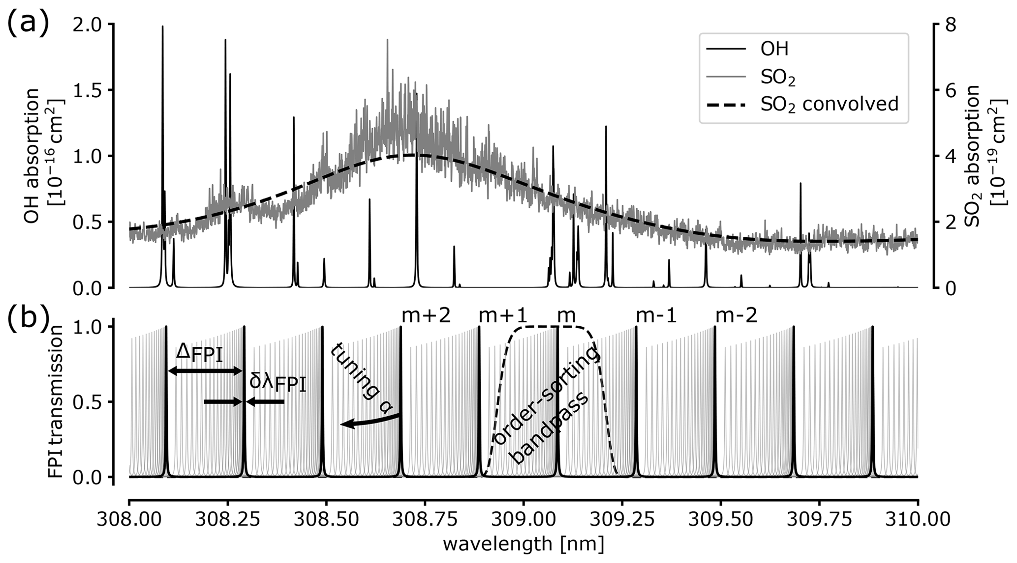
Figure 1(a) OH absorption cross section (left ordinate axis; Rothman et al., 2013) and SO2 absorption cross section (right ordinate axis; Rufus et al., 2003). The dashed line shows a convolution of the SO2 absorption with a Gaussian of 0.4 nm width. (b) An FPI transmission spectrum (black drawn line) as it is scanning across a short wavelength range (indicated by the grey lines) obtained by tuning an instrument parameter (here, the incidence angle α is tuned from 0 to 2∘ in 0.05∘ steps). The decrease in peak transmission is due to an assumed small beam divergence (0.005∘ half opening angle). An order-sorting bandpass is indicated by the dashed line isolating the FPI peak of order m.
Many other atmospheric trace gases show strong and structured absorption on the picometre scale. Besides sulfur dioxide (SO2; e.g. Rufus et al., 2003), formaldehyde (HCHO; e.g. Ernest et al., 2012), water (Rothman et al., 2013), and chlorine monoxide (ClO; Barton et al., 1984), Neuroth et al. (1991) found strong, discrete, and narrow bromine monoxide (BrO) absorption lines in the UV region. Using these much more detailed and specific spectral features of the trace gases could not only substantially increase the selectivity but also, in many cases, increase the sensitivity of DOAS measurements. Additionally, the absorption cross sections of isotopologues of some trace gases could be distinguished, similarly to the moderate-spectral-resolution measurements of water vapour isotopologues (e.g. Frankenberg et al., 2009). Figure 1a illustrates the addressed difference in spectral resolution by showing the high-resolution absorption cross section of SO2 (Rufus et al., 2003) as well as a convolution representing the absorption cross section as seen by a compact GS with a 0.4 nm spectral resolution.
Moderate-resolution scattered sunlight DOAS measurements largely undersample solar Fraunhofer lines (the width of which can also be in the picometre range). On the one hand, this introduces uncertainties in the effective spectral absorption of the trace gases (see e.g. Lampel et al., 2017); on the other hand, in most cases, it implies the need for a Fraunhofer reference spectrum. High-resolution spectra would allow a direct separation of Fraunhofer structures from narrow trace gas absorption structures; moreover, absolute atmospheric column densities of trace gases could be determined (rather than the column density relative to a reference spectrum).
1.3 Instrument mobility
A key point in the success of moderate-spectral-resolution DOAS measurements in the atmosphere is the use of compact and stable (i.e. mobile) spectrographs (volume of the order of 1 L, a focal length f of about 10 cm, and no moving parts). As mentioned above, they typically yield a resolving power of approximately 1000 and a light throughput that allows for the recording of scattered sunlight spectra in the UV and visible spectral range with a SNR of several thousand within less than a minute (e.g. Lauster et al., 2021). This is sufficient to retrieve many of the weakly absorbing atmospheric trace gases in the UV and visible spectral range (optical densities of ca. 0.01–0.0001) and to study their dynamics and chemistry.
The mobility of measurement equipment provides substantial advantages for practical field applications, including the following: (1) deployment on mobile platforms (e.g. cars, camels, drones, balloons, aircraft, and miniature satellites); (2) the significant reduction of costs for field campaigns due to reduced infrastructure and human resource requirements; (3) remote locations (e.g. deserts or volcanic craters) are made accessible (e.g. with backpack sized instruments); and (4) instruments can be employed in autonomous, remote, and low-maintenance measurement networks (see e.g. Galle et al., 2010; Arellano et al., 2021). In practice, these points are substantial factors making scientific environmental observations feasible.
As will be shown below, increasing the resolving power of a GS also requires a larger instrument size. Thus, the mobility advantages are largely lost. The use of FPIs in spectrograph set-ups can yield high resolving power while maintaining a high instrument mobility.
1.4 Fourier transform spectroscopy
This work focusses on spectrograph set-ups (GSs, FPI spectrographs) because of their high stability (no movable parts) and low sensitivity to fluctuations in light intensity. FTSs (i.e. Michelson interferometers) do not fulfil these requirements. A one-pixel detector records interferograms in a temporal sequence while mechanical changes in the optics (i.e. the interferometer path length) are conducted. This already imposes limitations on the mobility of the FTS as well as its applicability under more dynamical measurement conditions (e.g. cloudy skies). As (in addition to GSs) FTSs are in broader use in atmospheric remote sensing (mostly towards longer wavelengths, where the well-established and cost effective technology of silicon detector arrays can not be used anymore, i.e. above ca. 1100 nm), they shall nevertheless be briefly mentioned here.
In contrast to GSs and FPI spectrographs FTSs reach a large spectral coverage with very high and adjustable spectral resolution. This can be an important advantage for many atmospheric studies.
Notholt et al. (1997) compared the SNR of high-resolution (R≈300 000) FTS measurements to the SNR of GS measurements with a similar resolving power (Iwagami et al., 1995) for direct sunlight measurements at around 308 nm. It was found that the SNRs of the FTS and GS were similar for clear-sky conditions and worse for the FTS under hazy or slightly cloudy conditions. Thus, the advantages of FPI spectrographs regarding the SNR found below (see Sect. 3.2.3) are expected to similarly hold for an FPI spectrograph to FTS comparison. While the spectral coverage for the high resolution of FTSs is superior, mobility aspects (movable parts and large focal lengths in FTSs) clearly favour FPI spectrographs.
FPIs are very simple optical instruments that have been known for a long time. However, progress in manufacturing processes has led to largely improved instrument properties over the last few decades. An FPI consists of two plane-parallel reflective surfaces (mirrors; see Fig. 2a). As incident light is reflected back and fourth between these surfaces, the interference of transmitted and reflected partial beams leads to spectral transmission patterns determined by the optical path length between the two surfaces (see e.g. Perot and Fabry, 1899, and Vaughan, 1989, for details). This optical path length and the optical path difference Γ is determined by the physical separation of the reflective surfaces d, the refractive index n of the medium between the surfaces, and the angle of incidence α of the incoming light:
Thus, the transmission maximum (constructive interference) with the order m is centred at the wavelength
The free spectral range (FSR) ΔλFPI describes the spectral separation of two neighbouring transmission peaks (or fringes) and is related to a transmission peak's FWHM δλFPI via the finesse ℱ (see Fig. 1b):
Thus, the spectral resolution of an FPI transmission order (i.e. the spectral width of its ILF) is given by δλFPI. The isolation of a single FPI peak is desired for broadband light sources, unless the correlation of the FPI transmission spectrum with the trace gas spectrum can be exploited (as in e.g. Vargas-Rodríguez and Rutt, 2009, and Kuhn et al., 2014, 2019). An order-sorting bandpass (i.e. the isolation of a wavelength range containing a single FPI fringe; see Fig. 1b) can be achieved by a bandpass filter, further FPIs (or a combination of both; see e.g. Mack et al., 1963), or dispersive elements like a grating or a prism (e.g. Fabry and Buisson, 1908). The order-sorting bandpass needs to be in the range of the FSR of the FPI. Through Eq. (3), the spectral resolution δλFPI of an FPI spectrograph is thus limited by the FPI instrument's finesse and the order-sorting bandpass. The finesse of an FPI indicates the number of interfering partial beams and, thus, depends on the reflectivity, the alignment, and the quality of the FPI mirror surfaces across its clear aperture (CA; e.g. the diameter of usable circular aperture). Therefore, it is limited by the manufacturing process to a large extent. Nowadays, high finesse across larger CAs is reached by static, air-spaced FPI set-ups (i.e. FPIs with fixed d and low-thermal-expansion glass spacers). The spectral width of bandpass filters, which in principle also consist of a sequence of interference layers, is limited by manufacturing processes in a similar way. Thus, the measurement application and the available optical components determine the appropriate order-sorting technique.
In order to resolve different wavelengths, the FPI has to be operated within a range of varied physical parameters (d, n, or α), resulting in a spectral shift of the FPI transmission (as indicated in Fig. 1b). This can be implemented in different ways (see e.g. Vaughan, 1989). For high-finesse FPIs, pressure or temperature tuning (i.e. changing the refractive index n of the medium between the mirrors) or using the dependence on the incidence angle α is preferred. The variation in the mirror separation d across the FPI instrument's CA often limits the finesse by impacting the parallelism of the mirrors. An extremely precise tuning of d would be required. Pressure tuning requires one, for instance, to ramp the pressure inside the FPI. While this can only be done in a time sequence, the use of detector arrays allows one to observe different incidence angles α simultaneously in spectrograph implementations without moving parts. For the study of dynamic processes in the atmosphere, a static spectrograph set-up is highly preferred.
Generally, a static set-up (i.e. without moving parts) has a high mechanical stability and low maintenance requirements. This is demonstrated by moderate-resolution GS applications. Spectrographs using FPIs implemented with low-thermal-expansion glass (linear expansion coefficient ) spacers further yield superior thermal stability. From Eqs. (1) and (2), it follows that . A rather extreme temperature change of 10 K then induces a shift of the transmission spectrum by 10−7 λ. Even for a high resolving power of 105, the effect on the measurement would be negligible in most cases. The issue of potentially varying air density within the etalon impacting the refractive index is solved by hermetically sealing the etalon. Furthermore, the temperature impacts on FPIs, as well as the impact on the simple optics, can be accounted for in models of the instrument transmission. This is much more difficult for GSs, as temperature also significantly affects the rather non-linear imaging of the slit for these instruments. Thus, while GSs often require active temperature stabilisation (see e.g. Platt and Stutz, 2008), this might be redundant for most FPI spectrograph applications. This further substantially enhances their mobility through a simpler and smaller set-up with lower power consumption.
In the following, sample calculations are mostly made for short wavelengths (≈300 nm), where FPI manufacturing is most challenging. For increasing wavelengths, the inferred performance tends to improve because the absolute finesse-limiting requirements concerning the roughness, parallelism, or sphericity of the mirror surfaces (often given as fraction of wavelength, e.g. ) are higher for lower wavelengths.
FPI spectrograph implementation for atmospheric remote sensing
A simple and compact FPI spectrograph can be implemented with a static FPI as well as optics that image the different FPI incidence angles of the traversing light beam to concentric rings of equal FPI transmission on the focal plane (see Fig. 2a). There, a detector array records the intensities of the different spectral channels simultaneously. The spectral shift of the FPI transmission due to a small change in the small incidence angle α (i.e. a few hundredths of a radian, , cos α≈1) is dependent on the wavelength λm of the transmission peak of the order m and α itself (see Eqs. 1 and 2):
This demonstrates the non-linearity of the dispersion, which, however, leads to a constant light throughput for all spectral channels (as described in detail below). The wavelength range Λm covered by a particular transmission order (i.e. the FPI's spectral tuning range) is determined by the angle range covered by the parallelised light beam traversing the FPI:
The maximum and minimum incidence angles, αmax and αmin respectively, are determined by the illuminated entrance aperture B and the focal length of the collimating lens of the FPI spectrograph's imaging optics (lens 1; see Fig. 2a). For the imaging axis centred at the optical axis (αmin=0), the maximum incidence angle is
Assuming, for instance, an entrance aperture of B=3 mm and a focal length f1=50 mm, the maximum FPI incidence angle would be αmax=0.03 (or 1.72∘) and the spectral coverage would be about 0.135 nm at 300 nm. The practical incidence angle range that can be imaged onto the focal plane is in the range of a few degrees; therefore, the wavelength coverage can typically reach some hundreds of picometres in the near-UV. A moderate-resolution FPI spectrograph (with R≈1000, i.e. a spectral resolution of some hundreds of picometres at 300 nm) of the proposed implementation would exhibit a spectral coverage of the order of its spectral resolution, which would render it rather useless. This problem could be solved by tilting the FPI with respect to the imaging optical axis. Moderate-resolution FPI spectrographs are, however, not addressed in this study. For a resolving power of about 105, the 0.135 nm wavelength range at 300 nm would be divided into about 45 spectral channels with a 3 pm spectral resolution. This is about the number of spectral channels used in a typical moderate-resolution DOAS fitting window.
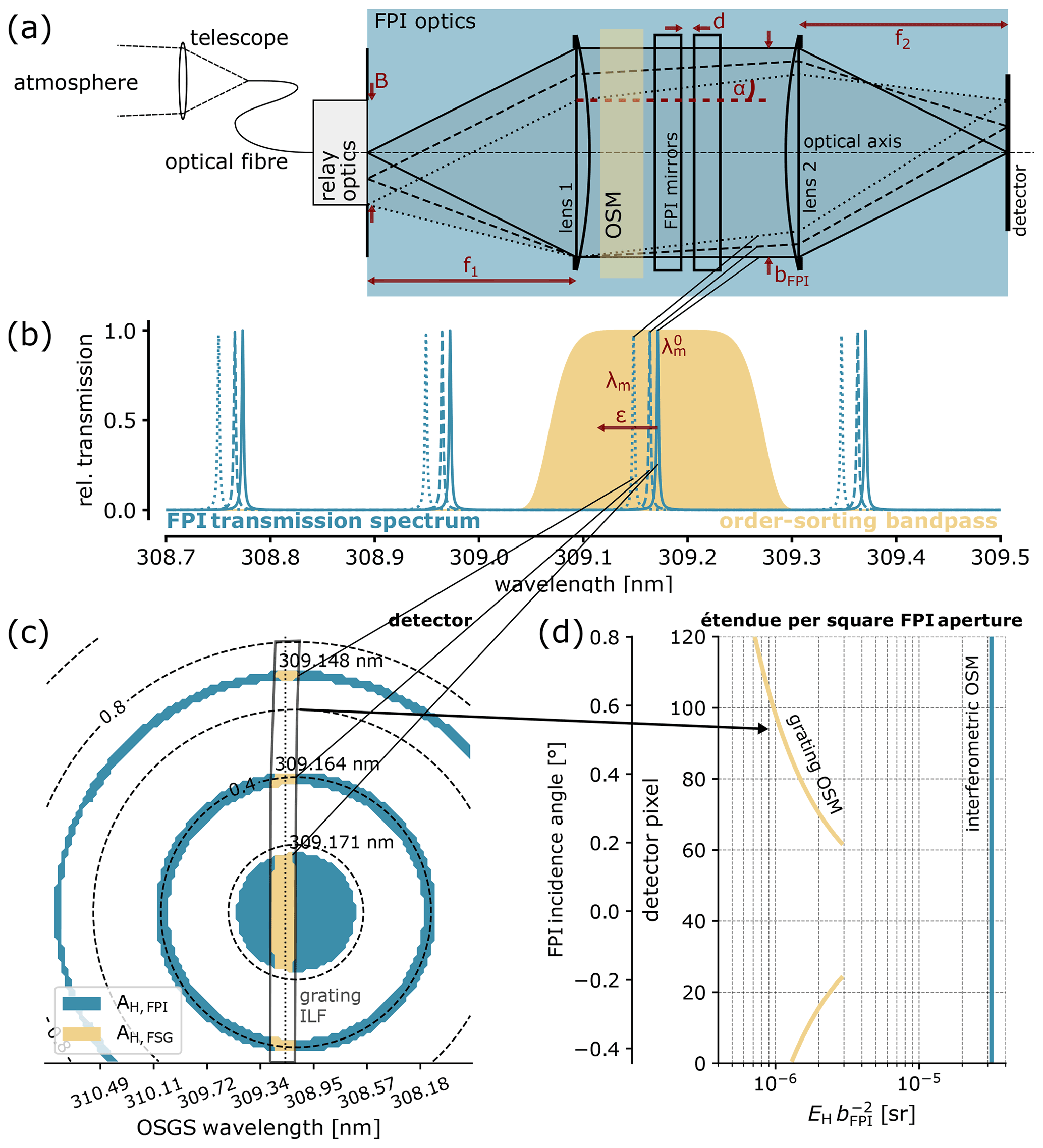
Figure 2Schematic optical set-up of an FPI spectrograph: (a) light from the atmosphere is directed to the spectrograph entrance via a telescope, an optical fibre, and, if needed, relay optics. The order-sorting mechanism (OSM), depending on its implementation, can be at different locations within the optical path. Lens 2 images the different FPI incidence angles onto the image plane; thus, different spectral FPI transmission spectra (b) are separated on the focal plane detector (c). The dashed circles in panel (c) indicate the corresponding FPI incidence angle α (in degrees). The OSM isolates a single FPI transmission order, either via filters (interferometric) or via a grating (see grating ILF in c). Panel (d) shows the étendue per square FPI aperture for the two OSMs and the instrument parameters in Table 1.
The sampling of the different spectral channels can be adjusted via the detector pixel size and the focal length of lens 2. Due to the non-linear dispersion, the sampling needs to be adjusted to the outermost ring corresponding to the spectral channel with the lowest wavelength of an FPI order (when assuming equally sized pixels). For the above example (B=3 mm, f1=50 mm) and f2=50 mm, the radial extension of the outermost spectral channel is about (see Eq. 4). Nowadays, detector pixels with a 1–5 µm pitch are common. This would facilitate sufficient sampling (>3.4 pixels per spectral channel width) for all spectral channels. The spectral sampling can further be adjusted via the focal length of lens 2. As the intensities of all pixels with the same wavelength are co-added, this does not affect the light throughput.
The above-mentioned order-sorting mechanisms (OSMs) allow two basic FPI spectrograph implementations:
-
Using a grating as the OSM in an FPI spectrograph results in a superposition of the linear grating dispersion with the radially symmetrical FPI transmission on the detector (see Fig. 2c). This allows one to record several FPI transmission orders at once, thereby increasing the total spectral coverage of the FPI spectrograph. This OSM is referred to as a grating OSM in the following.
-
Using a combination of further FPIs and filters as the OSM leads to an optimised étendue for a wavelength coverage of a single transmission order but also to a reduced total wavelength coverage (only a single FPI order). This OSM is referred to as interferometric OSM in the following.
As already mentioned above, the choice of the OSM depends on the measurement application, particularly the radiance of the light source, the desired SNR, the required spectral coverage, and the manufacturability of optical components.
An optical fibre and, as the case requires, relay optics direct the light collected by a telescope to the entrance aperture B (see Fig. 2a). From there, it traverses the imaging optics, containing the FPI and the OSM (certainly, the OSM can also be in front or behind the FPI imaging optics, for instance, the focal plane of an order-sorting GS could be re-imaged).
Both OSM implementations allow for simple, stable, and mobile set-ups with no moving parts. Therefore, they can be applied similarly to moderate-resolution compact grating spectrographs in field measurement campaigns, autonomous measurement networks in remote areas, and in airborne or satellite applications.
In this section, we compare the FPI spectrograph with the GS. First, size scaling considerations illustrate intrinsic mobility differences between FPI and grating instruments. Second, the light throughput per individual spectral channel is calculated and compared for different spectrograph implementations. Finally, from known SNRs of atmospheric measurements with moderate-resolution GSs, the SNRs of the high-resolution spectrographs are approximated.
3.1 Fundamental differences and size considerations
When examining spectroscopic methods, a basic question is how a physical parameter changes as a function of the wavelength λ. For spectrographs, this physical parameter is most often a deflection angle θ(λ) of a light beam. The angular dispersion describes the dependence of the deflection angle θg(λ) on the wavelength for the grating. For the FPI spectrograph, the incidence angle dependence of the FPI transmission spectrum is used to separate the different spectral channels (see Sect. 2). Therefore, we regard the incidence angle α as equivalent to the deflection angle θfp(λ) for the FPI.
For a blazed grating with a given ruling distance rg operated in the mth order and a Littrow-type spectrograph set-up (incidence angle and dispersion angle are as equal as possible), the relation of the wavelength and deflection angle θg (which equals the gratings blaze angle in this case) is given by (see e.g. Jacquinot, 1954)
consequently,
A close to ideal choice of the ruling distance of the grating for a given wavelength is rg≈m λ. For a typical value of , a small wavelength shift by the width δλ of one ILF (or one spectral channel) changes θg by
For the FPI, the angle dependence (for a small incidence angles) is given by Eq. (4):
The same small wavelength shift by one spectral channel δλ changes θfp by
This means that the angular change δθg for a single spectral channel of the GS is approximately given by its inverse resolving power, whereas for low FPI incidence angles, the angular change δθfp for a wavelength change of δλ can easily be 2 orders of magnitude larger than its inverse resolving power (e.g. factor of 100 for ).
In either type of spectrograph, the angular deflection is translated to a spatial separation δx on a detector array via the imaging optics with focal length f (see Fig. 3b or f2 in Fig. 2a):
The desired spatial interval per spectral channel on the detector depends on the pixel size and the spectral sampling. Assuming that the ILF is sampled by five pixels of 10 µm pitch, this interval would be δx=50 µm. Given that the size of a spectrograph is of the order of its focal length and its volume and mass scale with its third power (see e.g. Platt et al., 2021), the above relations reveal the principal difference between the GS and FPI spectrograph in terms of size and resolving power (see Fig. 3a). For instance, one could argue that easily portable tools for humans have the size of a human hand (i.e. ca. 10 cm), which is about the size of a CubeSat miniature satellite (see e.g. Poghosyan and Golkar, 2017). The resolving power of the corresponding GS is about 1000 and, thus, quite close to that used by moderate-resolution DOAS measurements. The resolving power of the corresponding (f=10 cm) FPI spectrograph is in the range of 105 and, therefore, capable of resolving individual rovibronic absorption lines of trace gases in the UV and visible spectral range.
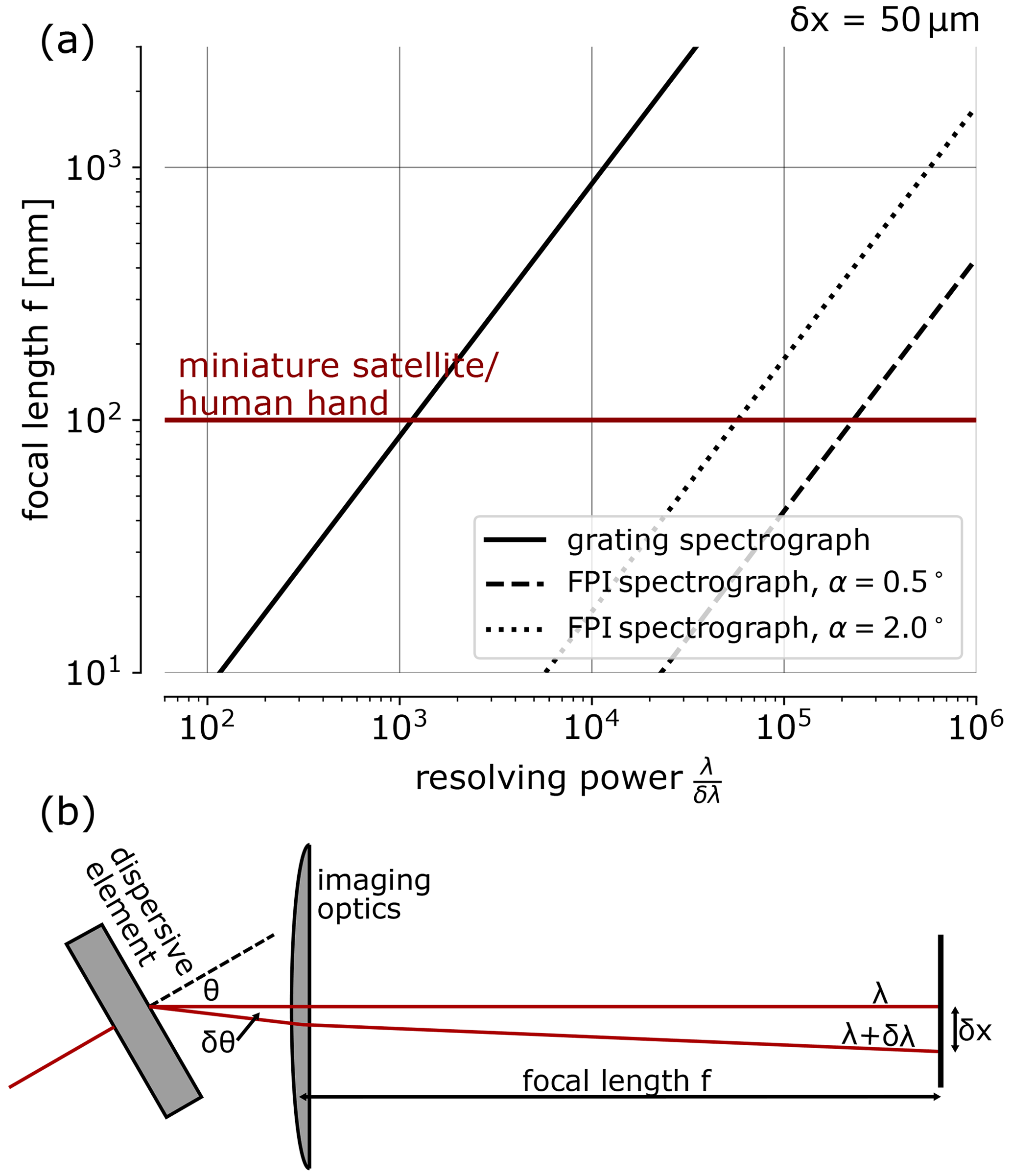
Figure 3(a) Relationship between size (represented by the focal length) and resolving power of GS and FPI spectrographs for an ILF spatial dimension of δx=50 µm. The size of a human hand or a miniature satellite is about 10 cm (red line); this size determines the favourable resolving power of the respective GS or FPI spectrograph for many applications. (b) Schematic of a spectrograph illustrating the fundamental aspects that determine the values in panel (a). The focal length f mainly determines the overall spectrograph size.
These considerations point towards the advantages of FPIs for high-resolution spectroscopy, where they have been widely in use for more than a century (see Vaughan, 1989). Moreover, we have illustrated that the fundamental differences between grating and FPI result in different instrument sizes (or levels of mobility) for a given resolving power. However, these considerations do not yet include the spectrograph's light throughput and, hence, the maximum achievable SNR, which is also decisive for most atmospheric remote sensing applications.
3.2 Light throughput
In the following, we derive the general relationship between the sensitivity of a spectroscopic measurement and the light throughput of a spectroscopic instrument. The light throughput kH of a spectrograph defines the conversion of incoming spectral radiance I (in units of []) to a flux Jph,H of photons with energies (or wavelengths) from within a single spectral channel of the spectrograph (see Eq. 16 below).
The upper limit for the SNR of an atmospheric remote sensing measurement is often determined by photoelectron shot noise, i.e. by the number of photons detected within an exposure time period δt (defining the measurement interval). The noise of such a spectrum is given by ; thus, the photon SNR Θ of a spectrum can be approximated by
This can be translated to the corresponding limits ΔS for the detection of trace gas column densities using the effective differential absorption cross sections , which, in many cases, are a function of spectral resolution (compare Fig. 1):
Here, the crucial role of the light throughput of the instrument becomes obvious, especially when the radiance of the light source (e.g. scattered sunlight) and the exposure time (e.g. time constant of the process to be studied) are fixed. Moreover, the choice of δλ is a compromise between optimal sensitivity (i.e. , typically decreasing with increasing δλ) and optimal light throughput (typically increasing with increasing δλ; see below). Particularly for trace gases with absorption cross sections consisting of discrete lines (e.g. OH, water vapour, or O2), the sensitivity increases almost linearly with the spectral resolution as long as it is much lower than the line width (see Appendix B).
When broadband light sources are used, a linear dependency of the light throughput on δλ is introduced. For line emitters where the spectral width of the emitted line is smaller than δλ (e.g. atomic emission lines), this is not the case (compare e.g. Jacquinot, 1954). Here, we regard light sources that are broadband compared to δλ (scattered or direct sunlight or incoherent artificial light sources); therefore, we include the factor δλ in the light throughput quantification. Furthermore, the light throughput depends on the geometric beam acceptance of the optics (i.e. its étendue EH), which often introduces a further δλ dependency (see the following subsections). The spectrograph's étendue for a given spectral channel is approximated by the product of surface area AH and the solid angle ΩH of the corresponding light beam:
Losses at the optical components are accounted for by a factor μ. From these effects, the light throughput can then be calculated as follows:
In the following, we compare the light throughput of FPI spectrographs with that of GSs for a given spectral resolution δλ. The losses at the optical components depend on their number, type, and quality. We assume that μ (accounting for these losses) is always optimised and that, apart from the OSM (introducing about a factor of 2 difference), there is no substantial difference in μ for the FPI spectrograph and GS. Thus, the light throughput is essentially determined by the étendue EH of an individual spectral channel.
We derive the étendue EH of GS and FPI spectrograph by approximating the surface area on the focal plane detector that is illuminated by light from a single spectral channel. The spectrograph's imaging optics determines the corresponding beam solid angle.
Imaging magnification does not affect the étendue (which is one of the reasons why the étendue is a universal measure of a spectrograph's quality), as it only converts a solid angle into surface area and vice versa. Therefore, for a light throughput comparison, we can ignore magnification and always assume ideal 1:1 imaging (i.e. collimating and focusing optics with the same focal length).
Investigating the light throughput per wavelength interval δλ allows the comparison of spectrograph set-ups with respect to their photon shot noise-limited SNR.
3.2.1 Étendue of a grating spectrograph
For a simple GS, as typically used for DOAS measurements, the above definition of EH might seem a bit artificial, as the étendue per spectral channel δλGS equals the étendue of the entrance optics. Assuming ideal 1:1 imaging, the surface area AH,GS on the detector that is illuminated by light from within δλGS is determined by the illuminated slit area (i.e. by the illuminated slit height hS and width wS). The slit width determines the spectral resolution via the GS's linear dispersion along the dispersion direction x. Because of the 1:1 imaging, AH,GS at the detector is given by
The corresponding imaging beam solid angle ΩH can be calculated from the F number of the GS's imaging optics, according to the approximation for higher F numbers:
with the imaging optics' (or the grating's) circular CA b and its focal length f. The étendue of a GS is then
In the spectral ranges regarded in this study, due to the availability of appropriate gratings, the GS resolving power is basically determined by slit imaging. When the grating is optimised to the operating wavelength (i.e. rg≈m λ, see above, or κ rg=m λ with κ≈1), the GS resolving power is determined by the slit width and focal length (see Appendix C for details):
Without exact knowledge of the factor κ (which is around unity and accounts for slight inaccuracies in the assumptions made) this relation allows one to evaluate how the size and the étendue of a particular GS change with its slit width and focal length for constant resolving power (see Fig. 4). As a measure of the spectrograph's size scaling, a minimum “beam volume” VGS is determined by the light cone constrained by the F number and the focal length:
While representing the lowest boundary for the absolute size of the spectrograph's optical set-up, it describes the scaling of a GS's volume and mass with the third power of its focal length for a constant F number (see also Platt et al., 2021).
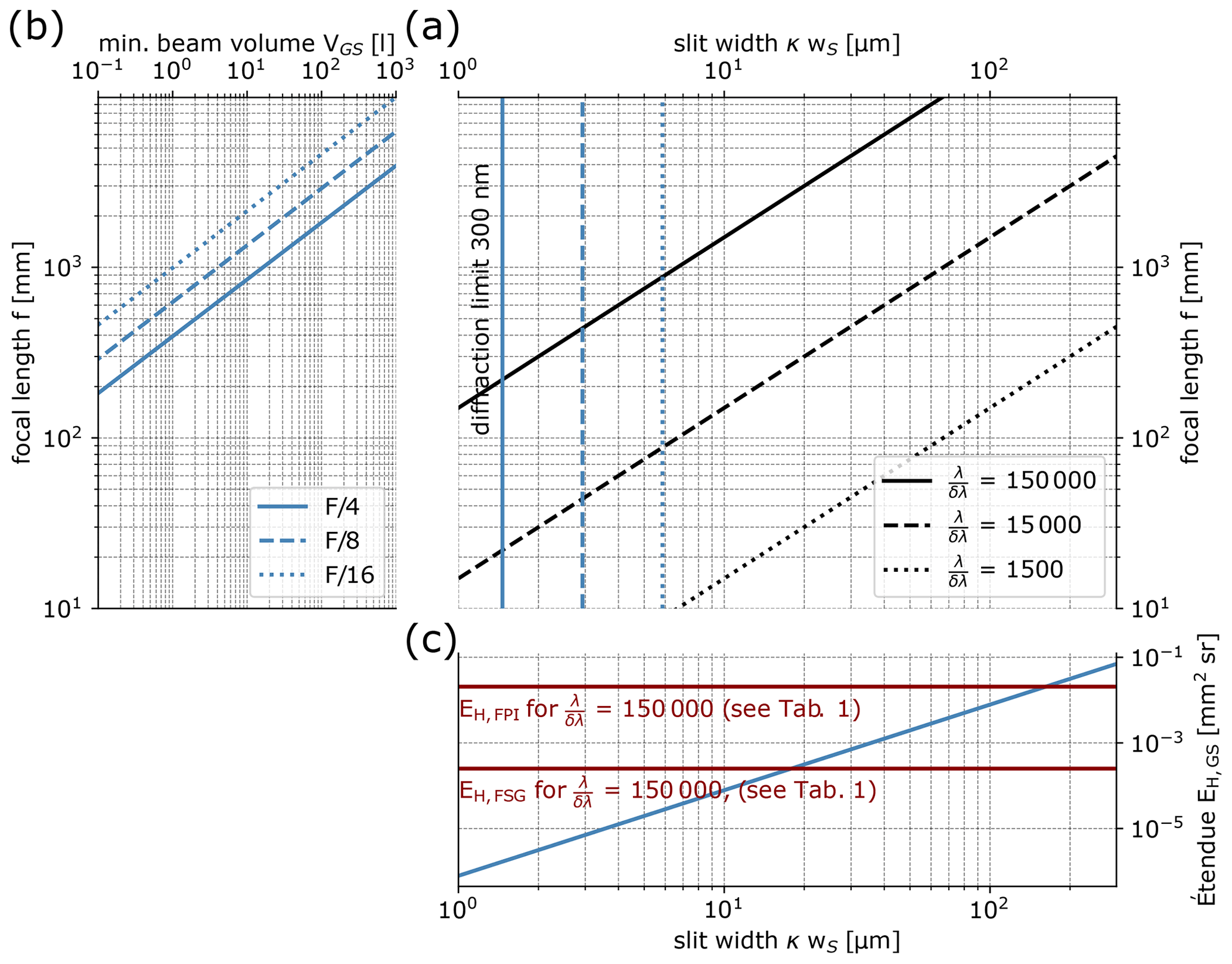
Figure 4Combined visualisation of Eqs. (20)–(22) and (24). (a) For three exemplary resolving powers (1500, 15 000, and 150 000), the possible slit-width-to-focal-length ratios are shown. The focal length determines the spectrograph's size scaling (b), whereas the slit width determines its étendue (blue line in c). The étendue of the FPI spectrograph with the grating OSM (for an incidence angle of 0.5∘) and the total étendue of the FPI (i.e. the FPI spectrograph with an interferometric OSM) with the specifications given in Table 1 are shown in red.
The resolving power of such an idealised GS can now be increased by either increasing the focal length or by narrowing the entrance slit (see Fig. 4). Increasing the focal length leads to a larger and heavier instrument and is, therefore, limited by mobility requirements. Narrowing the entrance slit reduces the étendue of the GS. The theoretical lower bound is given by diffraction at the entrance slit, i.e.
In practice, imaging aberrations limit the resolving power for narrow slit widths. In particular, aberrations will limit the slit height of the GS, which substantially influences the GS étendue (see Eq. 4). Approximating the maximum possible slit height based on an empirical quantification of the astigmatism of GSs by Fastie (1952) leads to the following simple expression (see Appendix D):
By inserting this relationship into Eq. (19), the expression for the GS étendue is further simplified to
Surprisingly, the F number cancels, which is because small F numbers increase the accepted beam solid angle of the GS while also reducing the allowed slit height through imaging aberrations (at the same time and by the same amount). In principle, this introduces a dependence of the GS étendue on the square of δλGS, which further stresses the problems of high-resolution GS. This does not mean that the F number can be chosen arbitrarily. To avoid further distortions, the slit height must remain much smaller than the CA of the imaging optics.
Correcting aberrations (like the astigmatism) is possible but onerous. Large imaging spectrographs can reach large slit heights with a low F number, for instance, by using lens optics to avoid off-axis imaging and, thus, largely reducing aberration (see e.g. Crisp et al., 2017). This will not be considered in this study, as we focus on mobile spectrographs.
3.2.2 Étendue of the FPI spectrographs
In order to assess the étendue of the FPI spectrographs, it is useful to first regard the étendue of a single FPI order, ignoring the influence of the OSM for the moment. For instance, an idealised bandpass filter or a FSR much larger than the spectral band of the light source could be assumed. By assessing the transmission solid angles ΩH,FPI of an FPI order (see Appendix E), we find the étendue of the FPI, which is (for a given resolving power) only dependent on the FPI CA bFPI:
Consequently, in the focal plane of a lens that is placed behind the FPI (lens 2 in Fig. 2a), the appearing rings corresponding to a wavelength interval δλFPI (Fig. 2c, d) have the same surface area and the étendue of all spectral channels is the same. For a given FPI CA and resolving power, EH,FPI (as given by Eq. 25) states an upper limit for the étendue of an FPI spectrograph.
For an FPI spectrograph with an interferometric OSM, this étendue can be reached if the étendue of all of the respective OSM components is equal or larger than EH,FPI. This should not be a problem, as the interferometric OSM components are FPIs or interference filters with similar or lower resolving powers and, therefore, higher étendue for the same CA (see Appendix G for details).
For the grating OSM, things are a bit more complicated. We assume an order-sorting GS (OSGS) with a spectral resolution of about the FPI's FSR (i.e. ). The spectrum of the OSGS can, for instance, be re-imaged by the FPI imaging optics (Fig. 2a). Therefore, the radially symmetric FPI spectral transmission overlaps with the OSGS spectrum, resulting in stripes (along the OSGS slit dimension) that isolate individual FPI transmission orders. Specifically, this will introduce an FPI incidence angle dependence to the étendue. The étendue of the FPI spectrograph with a grating OSM EH, FSG can be approximated by the following expression (see Appendix F):
As expected, the étendue equals the étendue of the OSGS with the slit height replaced by the radial extent of an FPI transmission ring with the spectral width of δλFPI. Furthermore, it can be expressed as a fraction of the total étendue (Eq. 25) of the used FPI. The expression approximates only a part of the total spectrum recorded with such an FPI spectrograph (i.e. where grating dispersion and FPI dispersion are approximately perpendicular). It is, however, representative for large parts of the spectrum.
The OSGS resolution δλOSGS needs to approximately equal the FSR ΔλFPI of the FPI. This means that the slit width wS of the OSGS (and, thus, EH,FSG) can be increased if the FSR of the FPI is increased. In order to keep the spectral resolution δλFPI constant, the same increase is required for the finesse. For increasing slit width, FSR, and finesse, EH,FSG converges to EH,FPI. As less FPI orders are then sampled, the total wavelength coverage decreases. This allows one, for instance, to adjust the spectral coverage and the étendue according to a specific application.
For Eq. (26) to hold, the F numbers of the OSGS and FPI imaging optics need to be matched. Thus, the focal length f2 is determined by the FPI's CA and the OSGS's F number. Figure 2c and d illustrate the étendue differences of the interferometric and grating OSM.
3.2.3 Comparison of FPI spectrographs and GSs
With the above evaluation of the étendue, we can compare the light throughput and SNR of FPI spectrographs with a GS for a given resolving power. Furthermore, we can relate the results to moderate-resolution GSs with a known absolute SNR. This allows one to approximate the absolute SNR of high-resolution FPI spectrographs for atmospheric remote sensing applications. Table 1 summarises the results.
In order to reach spectral resolutions of the order of single rotational trace gas absorption lines, a resolving power of 150 000 is assumed, which corresponds to a 2 pm spectral resolution at 300 nm. A 100 mm focal length facilitates the mobility of the spectrograph (Sect. 3.1). As found in Sect. 3.2.1 (see Fig. 4), the high-resolution GS can not be implemented with a 100 mm focal length (due to diffraction at the entrance slit) and, therefore, uses optics with a focal length of 1 m. We also assume the same F number of F=4 for all spectrographs. These assumptions mainly determine the étendue of the spectrographs.
Table 1Comparison of an FPI spectrograph and a GS. All spectrographs have an F number of 4 and, to ensure mobility, a focal length of 100 mm, except for the high-resolution GS (see Sect. 3.2.1 for details). The light throughput and SNR are calculated relative to that of a moderate-resolution GS, commonly used for DOAS measurements and, thus, with a known SNR.

For the FPI spectrograph with an interferometric OSM, we assume here that the element with the highest resolving power (i.e. the FPI with R=150 000) limits the étendue (see Eq. 25 and, for further details, Appendix G). The FPI spectrograph with a grating OSM requires the FSR of the FPI to be matched with the OSGS spectral resolution. We assume an FPI with a finesse of 100 and, therefore, need a OSGS with R=1500. A finesse of 100 for the given FPI dimensions is challenging but possible to manufacture for the UV. For larger wavelengths, even higher finesses (i.e. higher spectrograph light throughputs) can be reached. The étendue of the FPI spectrograph with a grating OSM was calculated for a representative FPI incidence angle of . For the light throughput comparison, the OSMs are accounted for by a loss factor of 0.5.
In practice, a moderate-resolution DOAS GS with f=75 mm typically has a resolving power of 600 (i.e. a spectral resolution of 0.5 nm at 300 nm), and a 100 µm wide slit is used with, for instance, a 400 µm optical fibre, determining the illuminated slit height (see e.g. Platt and Stutz, 2008). Such set-ups are able to record spectra of scattered sky light with SNRs of several thousand in the UV spectral range within about a 1 min integration time (see e.g. Lauster et al., 2021). In addition, we determined the light throughput of an (with respect to our formalism) optimised GS with the same moderate resolving power and a 100 mm focal length. Its light throughput is about an order of magnitude higher than that of moderate-resolution GSs presently in use.
Compared with compact moderate-resolution GSs that are in use for DOAS measurements, the FPI spectrograph with an interferometric OSM exhibits light throughput that is a factor of 100 lower with a 250 times higher spectral resolution. Consequently, for a given integration time, the photon SNR of the high-resolution spectrum of the FPI spectrograph is only about 10 times lower than that of a compact moderate-resolution GS. For the spectrum of a grating OSM FPI spectrograph, the corresponding SNR is 100 times lower for the same gain in spectral resolution. However, a considerably larger wavelength range is covered compared with the interferometric OSM version.
The high-resolution GS, despite its volume that is already about 1000 times the volume of the other spectrographs, yields even only about half the SNR of the grating OSM FPI spectrograph.
Extending the FPI's CA to 250 mm would yield a 250-fold increase in spectral resolution with the same SNR as a compact moderate-resolution DOAS spectrograph. If such an FPI could be manufactured, the corresponding spectrograph would have a focal length of about 1 m. The corresponding high-resolution GS with the same SNR would need a focal length of about 15 m.
4.1 Implications for atmospheric remote sensing
FPI spectrographs offer a way to reach large resolving powers with a largely reduced impact on the SNR (compared with GSs) while maintaining a mobile instrument set-up. This might allow substantially lower detection limits for trace gas measurements in the near-UV to NIR spectral range or may increase the measurements' spatial or temporal resolution.
When regarding noise-limited trace gas detection limits (as introduced in Eq. 14), we find that the effective differential absorption cross section (and, thus, the sensitivity of the measurement) increases with spectral resolution for many gases in the near-UV to NIR regions. For absorbers with discrete lines (e.g. OH, water vapour, or O2), the sensitivity increase will be almost linear to the increase in spectral resolution (see Appendix B, i.e. for our example a factor of ca. 250). For such gases, this effect outweighs the effect of reduced light throughput (0.01 compared with moderate-resolution GSs; Table 1), and the corresponding noise-limited detection limits of the FPI spectrograph with interferometric OSM will be reduced by a factor of (0.4 for a grating OSM) compared with that of common, moderate-spectral-resolution DOAS measurements. By reducing the temporal resolution of FPI spectrograph measurements by a factor of 100 (i.e. increasing the exposure time, e.g. from 30 s to 50 min), the same photon SNR as that of moderate-resolution DOAS measurements (with 30 s exposure time) can be reached, reducing the detection limits by another order of magnitude.
In addition, the increase in sensitivity comes with a massive increase in selectivity for the following reason: on the one hand, the high spectral resolution allows one to use much more specific absorption structures for gas detection; on the other hand, the high spectral resolution reduces or removes the influence of undersampled Fraunhofer lines for sunlight measurements. Thus, detection limits can further be significantly lowered with respect to moderate-resolution measurements, which are, in many cases, also limited by cross interferences (see e.g. Vogel et al., 2013). Consequently, line broadening effects could also add valuable information to retrievals of vertical atmospheric trace gas distributions, and the feasibility of distinguishing trace gas isotopologues is strongly improved. Besides improving water vapour isotopologue quantification (see e.g. Frankenberg et al., 2009), the separation of 34SO2 in volcanic emissions could also be possible using the differences in the absorption cross section, which are on a sub-nanometre scale (e.g. Danielache et al., 2008) and, thus, impossible to resolve with moderate spectral resolution.
Similar advantages are expected for the passive quantification of solar-induced fluorescence of chlorophyll by in-filling of narrow solar Fraunhofer lines with increased spectral resolution (see e.g. Plascyk and Gabriel, 1975; Grossmann et al., 2018).
The following simple example outlines the impact that FPI spectrographs might have on atmospheric sciences. According to the above assessment, a high-resolution FPI spectrograph records a spectrum with a SNR Θ of 3333 with about a 1 h integration time. For scattered sunlight measurements in the UV, the tropospheric light path L can reach about 10 km. The absorption cross section of OH at around 308 nm reaches about cm2 per molecule (see Rothman et al., 2013). The detection limit of OH concentrations ΔcOH (see Eq. 14) would then be
This is already in the range of tropospheric background OH concentrations (see e.g. Stone et al., 2012). This detection limit can be lowered further by using active light sources like light-emitting diodes (LEDs) or Xe lamps instead of scattered sunlight or by using larger FPIs or arrays of parallel FPI spectrographs.
Furthermore, as assessed in Sect. 1.4, FPI spectrographs are expected to have similar advantages over FTS and GS measurements in the NIR. Thus, FPI spectrographs could also substantially improve remote sensing measurements of greenhouse gases (e.g. CO2 or CH4) or CO in Earth's atmosphere. Instead of the large spectral coverage with high resolution reached by FTS, several FPI spectrographs could record spectra in different spectral windows that are relevant for the trace gas retrieval (e.g. an additional spectral window for O2 light path information; see e.g. Crisp et al., 2017).
An important aspect with respect to the named and quantified benefits of FPI spectrographs is that the low level of complexity and the high mobility of presently used moderate-resolution GS measurements is maintained.
4.2 FPI spectrograph prototype
As a proof of concept, we built a prototype of an FPI spectrograph with a grating OSM at the Institute of Environmental Physics in Heidelberg (see Fig. 5a). It operates at around 308 nm. An FPI with high finesse (ca. 95) across a CA of 5 mm and a resolving power of ca. 148 000 (supplied by SLS Optics Ltd) was used with a compact OSGS. We recorded a spectrum of light from a UV LED that traversed a burner flame (see Fig. 5a) containing large amounts of OH (typically several thousand parts per million; see e.g. Cattolica et al., 1982). For a light path of about 1 cm, this leads to optical densities >1 for many OH lines (see the OH absorption spectrum in Fig. 1, which is slightly altered due to the high temperature; see Rothman et al., 2013). Figure 5b shows the corresponding spectrum recorded by the FPI spectrograph prototype. The bright vertical stripes originate from a slight overlap of the individual FPI orders and, thus, also indicate their boundaries (compare Fig. 2b and c). The dark spots correspond to individual OH absorption lines. This is verified by calculating the intensity distribution using an instrument model and OH absorption data from Rothman et al. (2013). The orange box in Fig. 5b shows the region of the spectrum that is modelled in Fig. 5c. The locations of the individual OH absorption lines (dark spots) are clearly reproduced by the model, confirming the high resolving power.
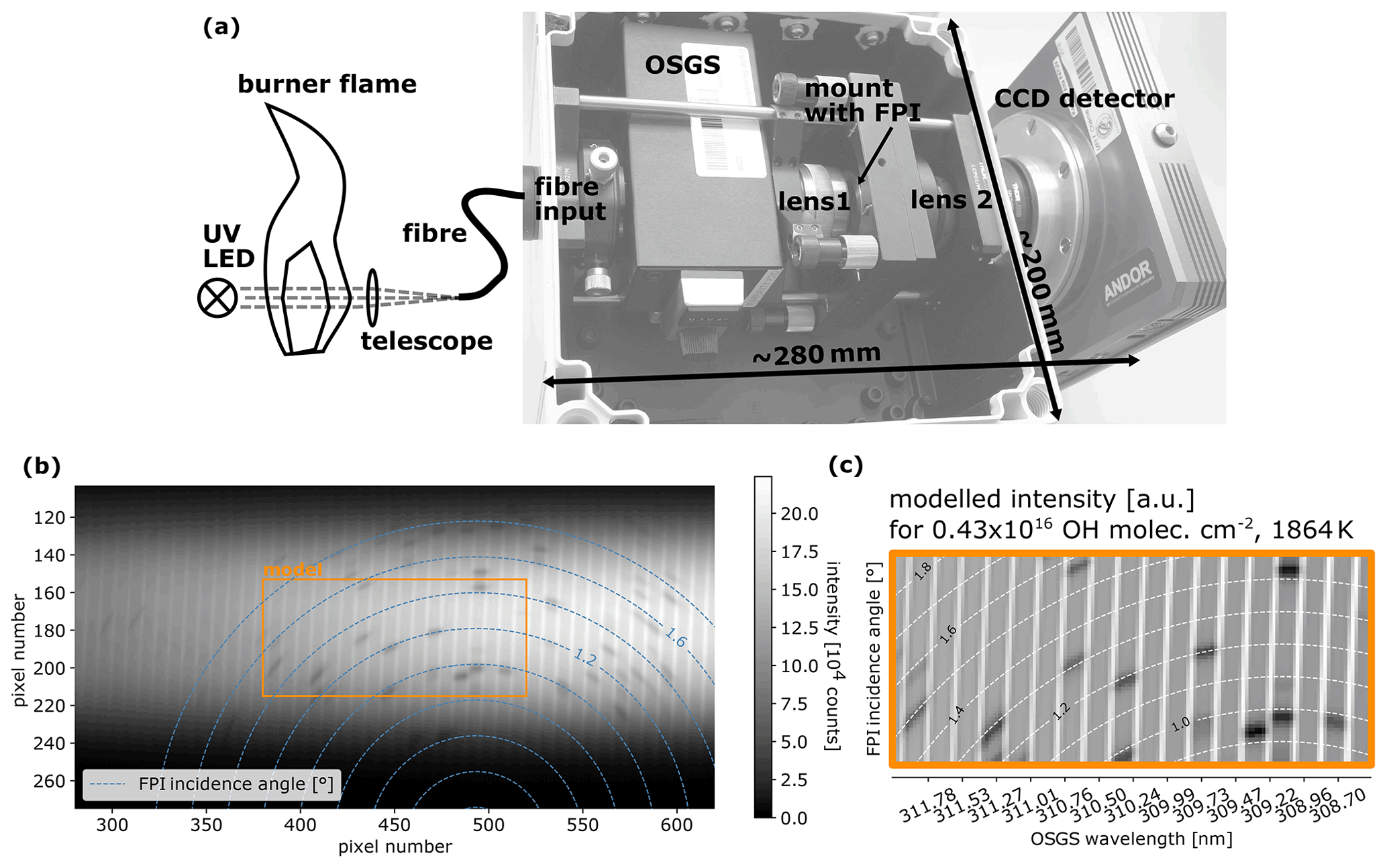
Figure 5Prototype of an FPI spectrograph with a grating OSM recording an absorption spectrum of OH in a burner flame. Panel (a) outlines the instrument and experimental set-up: light from a UV LED traverses a burner flame (containing a high amount of hot OH) before being directed to the FPI spectrograph via a telescope and a fibre. The FPI imaging optics re-image the moderate-resolution spectrum of the OSGS (compare Fig. 2). Panel (b) shows the recorded spectrum image: the vertical bright stripes arise from slight overlapping of FPI orders, dark spots indicate the individual OH absorption lines, and the dashed blue lines indicate rings of equal FPI incidence angle α. (c) Modelled intensities (using high-temperature OH absorption data from Rothman et al., 2013) for a part of the measured spectrum (orange box) with an instrument model show excellent agreement.
Compared with the FPI spectrograph assumed in Sect. 3.2.3, the light throughput of this prototype instrument is reduced due to its smaller CA (i.e. by a factor of about 25; see Eq. 25). The mobility advantages of FPI spectrographs as derived in Sect. 3.1 are already demonstrated by this still rudimentary prototype. Its volume is below 8 L, and it weighs less than 5 kg. The FPI can be replaced by an FPI with a larger CA without significantly impacting the instrument size.
A comprehensive description of this and further prototype instruments as well as the instrument models would go beyond the scope of this work and will be the topic of future publications.
We compared the performance of high-resolution spectrographs using gratings or FPIs. Increasing the spectral resolution of a GS results in the loss of its mobility and light throughput advantages and, thus, its applicability to many atmospheric studies. In contrast, the implementation of mobile FPI spectrographs with high resolving power is possible (as shown by the presented prototype) and can yield a much larger light throughput than a GS with the same (high) resolving power. Compared with moderate-resolution GSs (as used in conventional DOAS measurements), FPI spectrographs with the currently available optical components and a 250-fold spectral resolution (e.g. 2 pm instead of 0.5 nm at 300 nm) yield a light throughput that is only a factor of 100 smaller for an instrument of the same size. In contrast, the corresponding high-resolution GS, which can only be implemented with about a 1000-fold volume, yields only approximately of the moderate-resolution GS's light throughput.
Similarly to the resolving power luminosity product used by studies such as Jacquinot (1954) to generally compare FPIs to gratings, we can define a figure to quantify the applicability of spectroscopic instruments to atmospheric remote sensing studies with enhanced mobility requirements (e.g. measurements in remote areas or satellite instruments). This would then be the product of the resolving power and the square root of the light throughput (proportional to the inverse trace gas detection limits) per instrument volume. For a resolving power of 150 000, this figure is at least 3–4 orders of magnitude larger for FPI spectrographs compared with the GS.
On the one hand, the employment of mobile high-resolution FPI spectrographs would substantially increase the SNR of high-resolution measurements in the atmosphere; on the other hand, it would substantially increase the mobility of measurement instrumentation. These above-mentioned advantages basically come at the cost of spectral coverage of the spectrograph; however, for many applications, this should not be a problem.
The impact on atmospheric remote sensing measurements may be outlined with the following examples:
-
More trace gases (such as tropospheric OH) could be detectable using relatively simple passive or active absorption measurements.
-
In many cases, the detection limits of trace gases (e.g. SO2, H2O, HCHO, ClO, and BrO) routinely quantified by moderate-spectral-resolution DOAS measurements could be significantly lowered via the enhancement of sensitivity and selectivity due to the high spectral resolution.
-
Alternatively, the temporal or spatial resolution of such measurements could be enhanced.
-
From passive measurements using sunlight, absolute (rather than differential) column density measurements of trace gases absorbing in the UV and visible wavelength range could become possible (e.g. evaluation between Fraunhofer lines).
-
Due to the increase in the spectral resolution, the capability to separate trace gas isotopologue absorption is enhanced.
-
Line broadening could be quantified to add valuable information to the retrievals of vertical trace gas distributions.
-
Radiative transfer in haze or clouds can be studied with high-resolution measurements of O2 rotational lines.
-
Increased spectral resolution also enhances the sensitivity of chlorophyll fluorescence quantification through in-filling of Fraunhofer lines and similar studies.
-
FPI spectrographs are expected to similarly improve trace gas measurements in the NIR, as presently performed with FTS (e.g. quantification of green house gases in the atmosphere).
All in all, the results of this study suggest that high-resolution spectroscopy with mobile FPI spectrographs has the potential to substantially advance atmospheric trace gas remote sensing, thereby opening the door to many new insights into processes in Earth's atmosphere.
A1 List of abbreviations
| CA | Clear aperture |
| DOAS | Differential optical absorption spectroscopy |
| FPI | Fabry–Pérot interferometer |
| FSG | FPI spectrograph with a grating order-sorting mechanism |
| FSR | Free spectral range |
| FTS | Fourier transform spectroscopy |
| FWHM | Full width at half maximum |
| GS | Grating spectrograph |
| ILF | Instrument line function |
| NIR | Near-infrared |
| OSGS | Order-sorting grating spectrograph |
| OSM | Order-sorting mechanism |
| SNR | Signal-to-noise ratio |
| UV | Ultraviolet |
A2 List of symbols
| λ | Wavelength | ||
| δλ | Spectral resolution, spectral ILF FWHM | ||
| R | Resolving power | ||
| Γ | Optical path difference of the FPI | ||
| d | FPI mirror separation | ||
| n | Refractive index of the FPI medium | ||
| α | Incidence angle of light onto the FPI | ||
| m | Order of the FPI fringe or grating dispersion | ||
| λm | Wavelength at the FPI fringe with order m | ||
| ΔλFPI | FSR of the FPI | ||
| ℱ | Finesse of the FPI | ||
| γ | Linear thermal expansion coefficient | ||
| H | ILF | ||
| Λ | Wavelength coverage | ||
| B | Diameter of the circular entrance aperture | ||
| f | Focal length | ||
| θ | General dispersion deflection angle | ||
| δθ | Small, linearised change in θ | ||
| rg | Ruling distance of a grating | ||
| δx | Spatial separation in the focal plane through δθ | ||
| kH | Light throughput per spectral channel | ||
| I | Radiance | ||
| Jph,H | Photon flux per spectral channel | ||
| Nph | Number of photons | ||
| Θ | SNR | ||
| δt | Measurement interval, exposure time | ||
| ΔS | Detection limit for a trace gas (column density) | ||
| Effective absorption cross section of a trace gas | |||
| EH | Étendue per spectral channel | ||
| ΩH | Beam solid angle per spectral channel | ||
| AH | Surface area of beam cross section per spectral channel | ||
| μ | Factor accounting for losses at optical components | ||
| wS | Slit width | ||
| hS | Slit height | ||
| DGS | Linear dispersion of a GS | ||
| F | F number | ||
| b | CA | ||
| κ | Uncertainty factor around unity | ||
| V | Minimum beam volume of a spectrograph |
Here, we wish to demonstrate that the sensitivity of an absorption measurement with a spectrograph is, in most cases, strongly dependent on the spectral resolution. The sensitivity can be approximately quantified by the peak effective absorption cross section of a gas measured by an instrument with an ILF H:
where σ denotes the high-resolution absorption cross section, τ is the optical density, S is the column density of the gas, and the operator ⊗ represents the spectral convolution. The absorption of an isolated and sharp absorption line (see e.g. OH absorption cross section in Fig. 1) is diluted within the ILF of a spectrograph as long as its spectral resolution is lower than the width of the absorption line. In this case, increasing the spectral resolution results in a close to linear increase in sensitivity. This is illustrated by a simple example in Fig. B1, where we assume a 3 pm wide, Voigt-shaped absorption line and ILFs of different width modelled by sixth-order Gaussian curves.
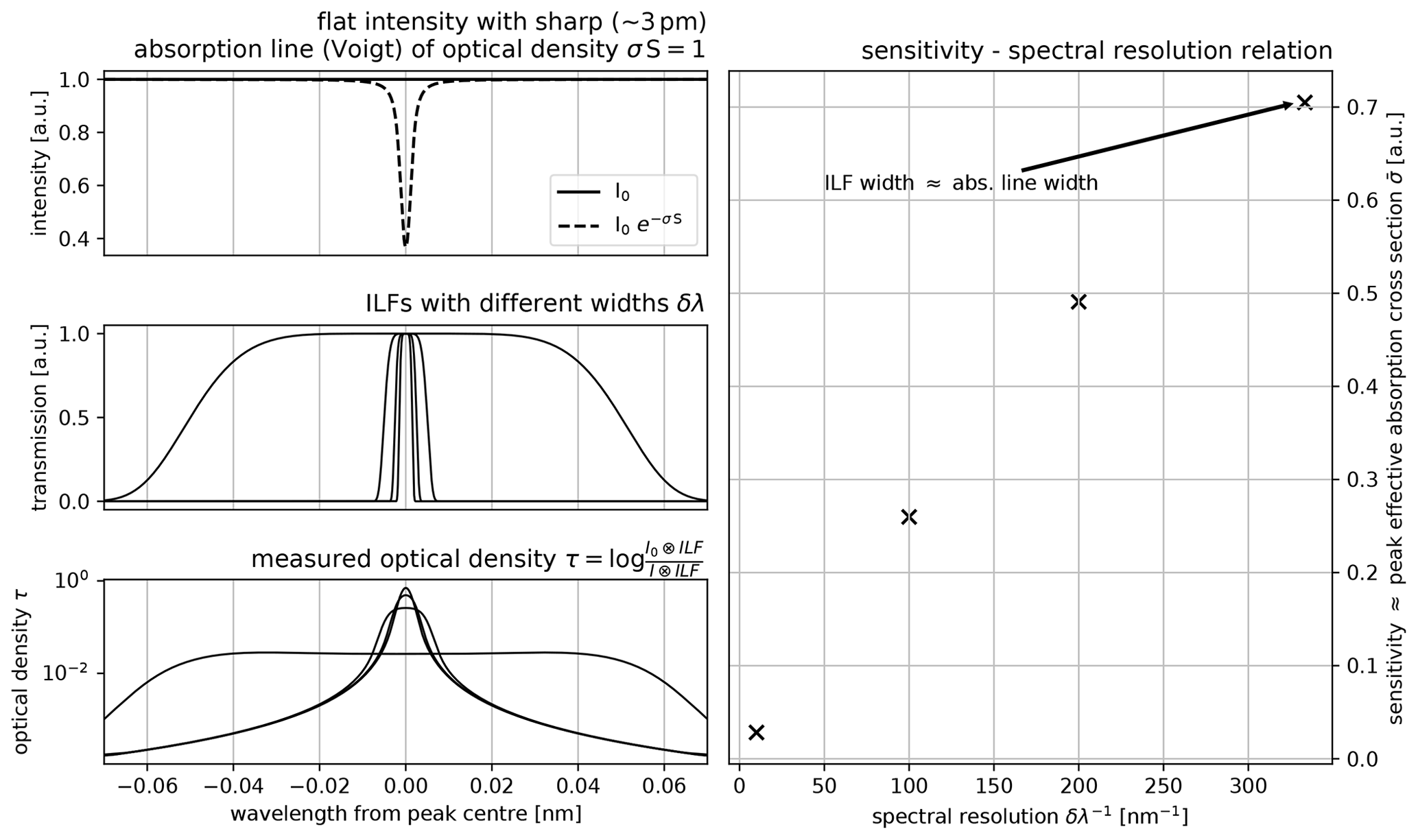
Figure B1The absorption of a sharp line is diluted throughout the ILF of the observing spectrograph. For ILF widths δλ that are much larger than the width of the absorption line, the measured absorption signal (peak optical density, i.e. peak effective absorption cross section ) increases approximately linearly with spectral resolution. For this visualisation, the ILF was modelled with a sixth-order Gaussian, and a Voigt profile was assumed for the absorption line.
The resolving power of the grating is limited by the number of illuminated grating rules Ng (i.e. ). This requires to be larger than the intended resolving power, which is almost always fulfilled by commonly used GS implementations. For an ideal choice of the grating, its effective ruling distance (see Eqs. 7 and 8) should be in the range of the measured wavelength. Gratings with that specification are available for all spectral ranges of interest for this study. Thus, one can conclude that the GS resolving power is generally limited by slit imaging. Here, we assume that , with κ being close to unity and accounting for any uncertainties in the assumptions. With the linear dispersion , we then find the following relation:
We will approximate the maximum possible slit height based on an empirical quantification of the astigmatism of GSs by Fastie (1952). The astigmatism is the deviation Δf of the focal length in the along- and across-slit directions, introduced by off-axis imaging with e.g. spherical mirrors. It is found to be proportional to the focal length and to the square of the angular distance ϕ of the slit to the normal of the focussing/collimating mirror. The entrance slit and the focal plane of the GS are separated by at least the grating's diameter b; hence, the lower limit of ϕ is given by . With that, the empirical astigmatism quantification of Fastie (1952) can be expressed using the focal length and F number of the GS:
The spread ΔL of an imaged point within the slit area along the defocussed astigmatism direction on the GS focal plane is then
As sharp imaging is only important in the dispersion direction for a GS, its optics are always focussed to the focal length in the across-slit direction. The astigmatism spread is then directed in the along-slit direction and is, therefore, negligible for the spectral imaging. However, due to the radial symmetry of the imaging mirrors, the across-slit component of the astigmatism increases with the distance from the slit centre (assuming the slit is centred at the imaging plane). For the ends of the slit, this component is given by the ratio of the slit height hS to the separation of the entrance slit and slit image, which equals at least the grating's CA b. This means that at the slit ends the slit image is widened by
When allowing for a slit widening by a 10th of the width of the slit image, we find the slit height to be limited to
If the FPI CA bFPI is illuminated with a divergent light beam, only light with a wavelength between (λm for α=0) and will be transmitted in the central beam part (limited by the incidence angle inducing a spectral shift of the FPI spectrum by δλFPI; see Fig. 2). Each wavelength interval corresponds to an incidence angle interval limiting the solid angle of the respective transmitted beam. Using Eqs. (1) and (2) and a cosine approximation, the incidence angle α corresponding to the transmission peak wavelength λm is determined as follows:
thus, for ,
Here, ϵ denotes the spectral displacement of λm with respect to (see Fig. 2b). The solid angle ΩH,FPI of a transmitted light beam with a wavelength between and (p being a positive real number) is then approximated by
This means that the transmission solid angle of an FPI for a wavelength interval δλFPI is independent of the incidence angle, and the étendue EH,FPI for a beam with a wavelength within δλFPI traversing the FPI CA () is
We can assume that the focal plane of an GS (i.e. its spectrum) is re-imaged with the FPI imaging optics (as that shown in Fig. 2a) with a matched F number. Furthermore, the spectral resolution of this order-sorting GS (OSGS) is matched to the FPI's FSR. The OSGS will cut out slices from the FPI ring system on the detector, where single FPI transmission orders are isolated (see Fig. 2d). The widths of these slices are given by the OSGS's ILF (i.e. its slit width). The result is a variable étendue across the FPI spectrograph's focal plane, generally decreasing with increasing distance to the centre of the ring system (i.e. increasing incidence angle α). In the following, an approximate quantification of the étendue EH,FSG of the FPI spectrograph with a grating OSM is derived. We thereby regard the area on the detector, where the rings of equal FPI transmission are approximately parallel to the grating dispersion dimension (e.g. a bit above the centre of the FPI ring system). There, the grating dispersion and the FPI dispersion are approximately perpendicular (see Fig. 2d). Light from within a wavelength interval δλFPI covers the area AH,FSG on the detector. For 1:1 imaging, its horizontal extent (in the grating dispersion direction) is given by the OSGS slit width wS.
The vertical extent of AH,FSG can again be approximated by the radial change in the detector location upon a shift of the transmission peak at λm by δλFPI. Thus, AH,FSG becomes a function of the imaging focal length f2=f1 and the angle range Δα required for tuning the FPI by δλFPI. Again, linearising Eq. (4) yields
This approximation should be fine for (see Eq. E2), where the FPI angular dispersion does not diverge. The product of Δα and the imaging focal length f2 is then the vertical extent of AH,FSG:
The solid angle of a light beam reaching a detector spot is again given by the imaging optics' F number (which should be matched to the OSGS's F number):
Finally, we obtain the étendue of the FPI spectrograph with a grating OSM:
In principle, the FPI can be used with a bandpass filter with a transmission FWHM of the FSR of the FPI. For an FPI with resolving power of R=150 000 and a finesse of ℱ=100, the bandpass FWHM should be around 0.2 nm in the UV at around 300 nm. Such filters with a transmission of about 25 %–35 % are available (see e.g. Klanner et al., 2021).
Alternatively, an additional FPI with lower resolving power can be used to increase the effective FSR and, thus, the required FWHM of the interference filter bandpass (as e.g. in Mack et al., 1963). The étendue will then still be limited by the FPI with the highest resolving power (see Eq. 25).
The resulting ring-shaped raw spectra are translated into linear spectra by co-adding the intensity of all of the pixels with the same distance to the centre of the ring system. Alternatively, a hardware-based circle-to-line converter (as e.g. proposed in Hays, 1990) can be used.
The spectrum shown in Fig. 5b can be obtained from the authors upon request.
JK conceptualised and conducted the theoretical study, built the prototype, and wrote the draft of the paper. All co-authors substantially contributed to the refinement of the study and revised the paper.
At least one of the (co-)authors is a member of the editorial board of Atmospheric Measurement Techniques. The peer-review process was guided by an independent editor, and the authors also have no other competing interests to declare.
Publisher's note: Copernicus Publications remains neutral with regard to jurisdictional claims in published maps and institutional affiliations.
The authors would like to thank SLS Optics Ltd for sharing their expertise in designing and manufacturing etalons.
This research has been partially funded by the German Science Foundation (DFG; project no. PL 193/23-1).
The article processing charges for this open-access publication were covered by the Max Planck Society.
This paper was edited by Alyn Lambert and reviewed by Ivan Prokhorov and two anonymous referees.
Arellano, S., Galle, B., Apaza, F., Avard, G., Barrington, C., Bobrowski, N., Bucarey, C., Burbano, V., Burton, M., Chacón, Z., Chigna, G., Clarito, C. J., Conde, V., Costa, F., De Moor, M., Delgado-Granados, H., Di Muro, A., Fernandez, D., Garzón, G., Gunawan, H., Haerani, N., Hansteen, T. H., Hidalgo, S., Inguaggiato, S., Johansson, M., Kern, C., Kihlman, M., Kowalski, P., Masias, P., Montalvo, F., Möller, J., Platt, U., Rivera, C., Saballos, A., Salerno, G., Taisne, B., Vásconez, F., Velásquez, G., Vita, F., and Yalire, M.: Synoptic analysis of a decade of daily measurements of SO2 emission in the troposphere from volcanoes of the global ground-based Network for Observation of Volcanic and Atmospheric Change, Earth Syst. Sci. Data, 13, 1167–1188, https://doi.org/10.5194/essd-13-1167-2021, 2021. a
Barton, S. A., Coxon, J. A., and Roychowdhury, U. K.: Absolute absorption cross sections at high resolution in the A2Πi−X2Πi band system of ClO, Can. J. Phys., 62, 473–486, https://doi.org/10.1139/p84-066, 1984. a
Burnett, C. R. and Burnett, E. B.: Spectroscopic measurements of the vertical column, abundance of hydroxyl (OH) in the earth's atmosphere, J. Geophys. Res., 86, 5185, https://doi.org/10.1029/jc086ic06p05185, 1981. a
Cattolica, R. J., Yoon, S., and Knuth, E. L.: OH Concentration in an Atmospheric-Pressure Methane-Air Flame from Molecular-Beam Mass Spectrometry and Laser-Absorption Spectroscopy, Combust. Sci. Technol., 28, 225–239, https://doi.org/10.1080/00102208208952557, 1982. a
Crisp, D., Pollock, H. R., Rosenberg, R., Chapsky, L., Lee, R. A. M., Oyafuso, F. A., Frankenberg, C., O'Dell, C. W., Bruegge, C. J., Doran, G. B., Eldering, A., Fisher, B. M., Fu, D., Gunson, M. R., Mandrake, L., Osterman, G. B., Schwandner, F. M., Sun, K., Taylor, T. E., Wennberg, P. O., and Wunch, D.: The on-orbit performance of the Orbiting Carbon Observatory-2 (OCO-2) instrument and its radiometrically calibrated products, Atmos. Meas. Tech., 10, 59–81, https://doi.org/10.5194/amt-10-59-2017, 2017. a, b
Danielache, S. O., Eskebjerg, C., Johnson, M. S., Ueno, Y., and Yoshida, N.: High-precision spectroscopy of 32S, 33S, and 34S sulfur dioxide: Ultraviolet absorption cross sections and isotope effects, J. Geophys. Res., 113, D17314, https://doi.org/10.1029/2007jd009695, 2008. a
Dorn, H.-P., Brandenburger, U., Brauers, T., Hausmann, M., and Ehhalt, D. H.: In-situ detection of tropospheric OH radicals by folded long-path laser absorption. Results from the POPCORN Field Campaign in August 1994, Geophys. Res. Lett., 23, 2537–2540, https://doi.org/10.1029/96gl02206, 1996. a
Ernest, C. T., Bauer, D., and Hynes, A. J.: High-Resolution Absorption Cross Sections of Formaldehyde in the 30285–32890 cm−1 (304–330 nm) Spectral Region, J. Phys. Chem. C, 116, 5910–5922, https://doi.org/10.1021/jp210008g, 2012. a
Fabry, C. and Buisson, H.: Wavelength measurements for the establishment of a system of spectroscopic standards, Astrophys. J., 27, 169–196, 1908. a
Fastie, W. G.: Image forming properties of the Ebert monochromator, J. Opt. Soc. Am., 42, 647–651, 1952. a, b, c
Frankenberg, C., Yoshimura, K., Warneke, T., Aben, I., Butz, A., Deutscher, N., Griffith, D., Hase, F., Notholt, J., Schneider, M., Schrijver, H., and Rockmann, T.: Dynamic Processes Governing Lower-Tropospheric HDOH2O ratios as Observed from Space and Ground, Science, 325, 1374–1377, https://doi.org/10.1126/science.1173791, 2009. a, b
Galle, B., Johansson, M., Rivera, C., Zhang, Y., Kihlman, M., Kern, C., Lehmann, T., Platt, U., Arellano, S., and Hidalgo, S.: Network for Observation of Volcanic and Atmospheric Change (NOVAC) – A global network for volcanic gas monitoring: Network layout and instrument description, J. Geophys. Res., 115, D05304, https://doi.org/10.1029/2009JD011823, 2010. a
Grossmann, K., Frankenberg, C., Magney, T. S., Hurlock, S. C., Seibt, U., and Stutz, J.: PhotoSpec: A new instrument to measure spatially distributed red and far-red Solar-Induced Chlorophyll Fluorescence, Remote Sens. Environ., 216, 311–327, https://doi.org/10.1016/j.rse.2018.07.002, 2018. a
Hays, P. B.: Circle to line interferometer optical system, Appl. Optics, 29, 1482, https://doi.org/10.1364/ao.29.001482, 1990. a
Hübler, G., Perner, D., Platt, U., Tönnissen, A., and Ehhalt, D. H.: Groundlevel OH radical concentration: New measurements by optical absorption, J. Geophys. Res., 89, 1309–1319, https://doi.org/10.1029/jd089id01p01309, 1984. a
Iwagami, N., Inomata, S., Murata, I., and Ogawa, T.: Doppler detection of hydroxyl column abundance in the middle atmosphere, J. Atmos. Chem., 20, 1–15, https://doi.org/10.1007/bf01099915, 1995. a, b
Jacquinot, P.: The Luminosity of Spectrometers with Prisms, Gratings, or Fabry-Perot Etalons, J. Opt. Soc. Am., 44, 761–765, https://doi.org/10.1364/josa.44.000761, 1954. a, b, c, d
Jacquinot, P.: New developments in interference spectroscopy, Rep. Prog. Phys., 23, 267–312, https://doi.org/10.1088/0034-4885/23/1/305, 1960. a, b
Klanner, L., Höveler, K., Khordakova, D., Perfahl, M., Rolf, C., Trickl, T., and Vogelmann, H.: A powerful lidar system capable of 1 h measurements of water vapour in the troposphere and the lower stratosphere as well as the temperature in the upper stratosphere and mesosphere, Atmos. Meas. Tech., 14, 531–555, https://doi.org/10.5194/amt-14-531-2021, 2021. a
Kuhn, J., Bobrowski, N., Lübcke, P., Vogel, L., and Platt, U.: A Fabry–Perot interferometer-based camera for two-dimensional mapping of SO2 distributions, Atmos. Meas. Tech., 7, 3705–3715, https://doi.org/10.5194/amt-7-3705-2014, 2014. a
Kuhn, J., Platt, U., Bobrowski, N., and Wagner, T.: Towards imaging of atmospheric trace gases using Fabry–Pérot interferometer correlation spectroscopy in the UV and visible spectral range, Atmos. Meas. Tech., 12, 735–747, https://doi.org/10.5194/amt-12-735-2019, 2019. a
Lampel, J., Wang, Y., Hilboll, A., Beirle, S., Sihler, H., Puķīte, J., Platt, U., and Wagner, T.: The tilt effect in DOAS observations, Atmos. Meas. Tech., 10, 4819–4831, https://doi.org/10.5194/amt-10-4819-2017, 2017. a
Lauster, B., Dörner, S., Beirle, S., Donner, S., Gromov, S., Uhlmannsiek, K., and Wagner, T.: Estimating real driving emissions from multi-axis differential optical absorption spectroscopy (MAX-DOAS) measurements at the A60 motorway near Mainz, Germany, Atmos. Meas. Tech., 14, 769–783, https://doi.org/10.5194/amt-14-769-2021, 2021. a, b
Mack, J. E., McNutt, D. P., Roesler, F. L., and Chabbal, R.: The PEPSIOS Purely Interferometric High-Resolution Scanning Spectrometer I The Pilot Model, Appl. Optics, 2, 873–885, https://doi.org/10.1364/ao.2.000873, 1963. a, b
Neuroth, R., Dorn, H. P., and Platt, U.: High resolution spectral features of a series of aromatic hydrocarbons and BrO: Potential interferences in atmospheric OH-measurements, J. Atmos. Chem., 12, 287–298, https://doi.org/10.1007/bf00048077, 1991. a
Notholt, J., Schütt, H., and Keens, A.: Solar absorption measurements of stratospheric OH in the UV with a Fourier-transform spectrometer, Appl. Optics, 36, 6076–6082, https://doi.org/10.1364/ao.36.006076, 1997. a, b
Perner, D., Ehhalt, D. H., Pätz, H. W., Platt, U., Röth, E. P., and Volz, A.: OH – Radicals in the lower troposphere, Geophys. Res. Lett., 3, 466–468, https://doi.org/10.1029/gl003i008p00466, 1976. a
Perot, A. and Fabry, C.: On the Application of Interference Phenomena to the Solution of Various Problems of Spectroscopy and Metrology, Astrophys. J., 9, 87, https://doi.org/10.1086/140557, 1899. a
Pfeilsticker, K., Erle, F., Funk, O., Veitel, H., and Platt, U.: First geometrical pathlengths probability density function derivation of the skylight from spectroscopically highly resolving oxygen A-band observations: 1. Measurement technique, atmospheric observations and model calculations, J. Geophys. Res.-Atmos., 103, 11483–11504, https://doi.org/10.1029/98jd00725, 1998. a
Plascyk, J. A. and Gabriel, F. C.: The Fraunhofer Line Discriminator MKII-An Airborne Instrument for Precise and Standardized Ecological Luminescence Measurement, IEEE T. Instrum. Meas., 24, 306–313, https://doi.org/10.1109/tim.1975.4314448, 1975. a
Platt, U. and Stutz, J.: Differential optical absorption spectroscopy, Springer Verlag, Berlin, Heidelberg, ISBN: 978-3-540-75776-4, 2008. a, b, c, d, e
Platt, U., Rateike, M., Junkermann, W., Rudolph, J., and Ehhalt, D. H.: New tropospheric OH measurements, J. Geophys. Res., 93, 5159–5166, https://doi.org/10.1029/jd093id05p05159, 1988. a
Platt, U., Wagner, T., Kuhn, J., and Leisner, T.: The “ideal” spectrograph for atmospheric observations, Atmos. Meas. Tech., 14, 6867–6883, https://doi.org/10.5194/amt-14-6867-2021, 2021. a, b
Poghosyan, A. and Golkar, A.: CubeSat evolution: Analyzing CubeSat capabilities for conducting science missions, Prog. Aerosp. Sci., 88, 59–83, https://doi.org/10.1016/j.paerosci.2016.11.002, 2017. a
Rothman, L., Gordon, I., Babikov, Y., Barbe, A., Benner, D. C., Bernath, P., Birk, M., Bizzocchi, L., Boudon, V., Brown, L., Campargue, A., Chance, K., Cohen, E., Coudert, L., Devi, V., Drouin, B., Fayt, A., Flaud, J.-M., Gamache, R., Harrison, J., Hartmann, J.-M., Hill, C., Hodges, J., Jacquemart, D., Jolly, A., Lamouroux, J., Roy, R. L., Li, G., Long, D., Lyulin, O., Mackie, C., Massie, S., Mikhailenko, S., Müller, H., Naumenko, O., Nikitin, A., Orphal, J., Perevalov, V., Perrin, A., Polovtseva, E., Richard, C., Smith, M., Starikova, E., Sung, K., Tashkun, S., Tennyson, J., Toon, G., Tyuterev, V., and Wagner, G.: The HITRAN2012 molecular spectroscopic database, J. Quant. Spectrosc. Ra., 130, 4–50, https://doi.org/10.1016/j.jqsrt.2013.07.002, 2013. a, b, c, d, e, f
Rufus, J., Stark, G., Smith, P. L., Pickering, J. C., and Thorne, A. P.: High-resolution photoabsorption cross section measurements of SO2, 2: 220 to 325 nm at 295 K, J Geophys. Res., 108, 5011, https://doi.org/10.1029/2002je001931, 2003. a, b, c
Stone, D., Whalley, L. K., and Heard, D. E.: Tropospheric OH and HO2 radicals: field measurements and model comparisons, Chem. Soc. Rev., 41, 6348–6404, https://doi.org/10.1039/c2cs35140d, 2012. a
Vargas-Rodríguez, E. and Rutt, H.: Design of CO, CO2 and CH4 gas sensors based on correlation spectroscopy using a Fabry–Perot interferometer, Sensor. Actuat. B-Chem., 137, 410–419, https://doi.org/10.1016/j.snb.2009.01.013, 2009. a
Vaughan, M.: The Fabry-Perot Interferometer History, Theory, Practice and Applications, CRC Press, Boca Raton, ISBN 9780852741382, 1989. a, b, c, d
Vogel, L., Sihler, H., Lampel, J., Wagner, T., and Platt, U.: Retrieval interval mapping: a tool to visualize the impact of the spectral retrieval range on differential optical absorption spectroscopy evaluations, Atmos. Meas. Tech., 6, 275–299, https://doi.org/10.5194/amt-6-275-2013, 2013. a
- Abstract
- Introduction
- High-resolution spectroscopy with Fabry–Pérot interferometers
- Comparison of the FPI spectrograph and GS
- Implications for atmospheric remote sensing, and the FPI spectrograph prototype developed in this study
- Conclusions
- Appendix A
- Appendix B: Relation between sensitivity and spectral resolution
- Appendix C: The GS resolving power is mainly limited by slit imaging
- Appendix D: Aberration-limited slit height of a compact GS
- Appendix E: The étendue of an FPI
- Appendix F: Étendue of an FPI spectrograph with a grating OSM
- Appendix G: On the implementation of the interferometric OSM
- Data availability
- Author contributions
- Competing interests
- Disclaimer
- Acknowledgements
- Financial support
- Review statement
- References