Biomass burning nitrogen dioxide emissions derived from space with TROPOMI: methodology and validation

Smoke from wildfires is a significant source of air pollution, which can adversely impact air quality and ecosystems downwind. With the recently increasing intensity and severity of wildfires, the threat to air quality is expected to increase. Satellite-derived biomass burning emissions can fill in gaps in the absence of aircraft or ground-based measurement campaigns and can help improve the online calculation of biomass burning emissions as well as the biomass burning emissions inventories that feed air quality models. This study focuses on satellite-derived NO_x emissions using the high-spatial-resolution TROPOspheric Monitoring Instrument (TROPOMI) NO₂ dataset. Advancements and improvements to the satellite-based determination of forest fire NO_x emissions are discussed, including information on plume height and effects of aerosol scattering and absorption on the satellite-retrieved vertical column densities. Two common top-down emission estimation methods, (1) an exponentially modified Gaussian (EMG) and (2) a flux method, are applied to synthetic data to determine the accuracy and the sensitivity to different parameters, including wind fields, satellite sampling, noise, lifetime, and plume spread. These tests show that emissions can be accurately estimated from single TROPOMI overpasses. The effect of smoke aerosols on TROPOMI NO₂ columns (via air mass factors, AMFs) is estimated, and these satellite columns and emission estimates are compared to aircraft observations from four different aircraft campaigns measuring biomass burning plumes in 2018 and 2019 in North America. Our results indicate that applying an explicit aerosol correction to the TROPOMI NO₂ columns improves the agreement with the aircraft observations (by about 10 %–25 %). The aircraft- and satellite-derived emissions are in good agreement within the uncertainties. Both top-down emissions methods work well; however, the EMG method seems to output more consistent results and has better agreement with the aircraft-derived emissions. Assuming a Gaussian plume shape for various biomass burning plumes, we estimate an average NO_x e-folding time of 2 ±1 h from TROPOMI observations. Based on chemistry transport model simulations and aircraft observations, the net emissions of NO_x are 1.3 to 1.5 times greater than the satellite-derived NO₂ emissions. A correction factor of 1.3 to 1.5 should thus be used to infer net NO_x emissions from the satellite retrievals of NO₂.

1 Introduction

Wildfires are a significant source of aerosols and trace gases in the global atmosphere (Andreae, 2019, and references therein). Exposure to wildfire smoke has been associated with adverse health impacts and premature mortality (Matz et al., 2020). The health impacts are generally greater in close proximity to active fire areas; however, health impacts are also associated with long-range transport of smoke plumes (Matz et al., 2020). In recent years, the number of wildfires has increased (e.g. Romero-Lankao et al., 2014; Landis et al., 2018), primarily driven by droughts, higher temperatures, and fuel loading caused by tree death (e.g. Kitzberger et al., 2007; Littell et al., 2009; Westerling, 2016). Studies suggest the intensity of fires may continue to rise, driven by climate change and its associated droughts, higher temperatures, and an earlier spring season (Liu et al., 2013; Wotton et al., 2017). This increase in wildfires, combined with the focus on national emission targets and air quality monitoring, leads to an increasing demand for improved knowledge of wildfire emissions.

One type of pollutants emitted by wildfires is nitrogen oxides (NO_x= NO₂ + NO), which have adverse effects on the environment and human health (Health Canada, 2018). NO_x plays a significant role in the tropospheric production of ozone and can contribute to acid rain. Wildfire emissions of NO_x exhibit large year-to-year variability and on average account for approximately 15 % of the global NO_x budget (Denman et al., 2007). The amount of nitrogen (N) released by wildfires strongly depends on the type of fuel being consumed (fuel nitrogen content) and the burning phase represented by the relative amounts of flaming and smoldering combustion. NO_x is primarily emitted during flaming combustion at high temperatures, whereas the release of reduced forms of nitrogen, such as NH₃, is favoured during the lower-temperature smoldering phase (e.g. Goode et al., 2000; Burling et al., 2010; Roberts et al., 2020). Reactive nitrogen species are released through fuel pyrolysis, if the fire temperatures are below ∼1200 ^∘C (Roberts et al., 2020, and references therein), where radical chemistry within the flames converts these fuel N to oxidized nitrogen species and N₂ (Ren and Zhao, 2012; Roberts et al., 2020). Each wildfire is a mixture of different stages of combustion that can occur simultaneously or at various times and locations within a given wildfire perimeter (Lindaas et al., 2021, and references therein).

A few species can be observed by satellite instruments and used to estimate fire emissions. Satellite remote-sensing observations have the advantage of continuous, near-global coverage, if meteorological conditions are favourable (e.g. clear sky) and the emissions are above the instrument's detection limit. Ground-based and aircraft measurements are difficult to obtain near the fire source (due to Temporary Flight Restriction zones), and field campaigns are infrequent with limited spatial coverage, while satellite-borne observations can be used to constrain wildfire emissions and can provide emission estimates for fires missed by measurement campaigns. Satellite-derived emissions can be derived using a variety of approaches, such as through the use of an inverse model or by directly using a mass balance or curve-fitting approach (de Foy et al., 2014). This study focuses on deriving the biomass burning emissions directly from satellite observations without the use of model simulations. Previously, de Foy et al. (2014) tested several different top-down emission estimation methods on synthetic data and concluded that emissions can be estimated accurately within 5 %–40 %, across all methods. Global NO_x emissions were first derived from satellite observations nearly 20 years ago by using a simple mass balance technique (Leue et al., 2001; Martin et al., 2003) applied to data from the Global Ozone Monitoring Experiment (GOME), 1995–2011, with a pixel size of 40×320 km² (Burrows et al., 1999). As satellites improved so did space-borne emission estimates, and in 2011 NO_x emissions were derived for the first time on a city-wide scale (Beirle et al., 2011) using observations from the Ozone Monitoring Instrument (OMI; 2004–present; 13×24 km²; at nadir; Levelt et al., 2006; Krotkov et al., 2016). NO_x emissions from large fires have also been derived from OMI observations (e.g. Mebust et al., 2011; Mebust and Cohen, 2014; Adams et al., 2019). More recently, Jin et al. (2021) reported NO_x emissions from biomass burning using NO₂ observations from the TROPOspheric Monitoring Instrument (TROPOMI) instrument.

Good spatio-temporal coverage and high spatial resolution enables a detailed plume shape, which is the key to accurately estimating fire emissions from satellite observations. With the recent advances in satellite-borne remote-sensing instruments, in terms of spatial resolution, as well as data product quality of the recorded spectra, top-down emission estimates can be improved. TROPOMI, launched in October 2017, has a high enough spatial resolution (3.5 km×5.5 km after 6 August 2019​​​​​​​; 3.5 km×7 km prior to August 2019) that makes it possible to resolve single plumes (Griffin et al., 2019), and with this, satellite-borne remote-sensing observations have entered a new era. The ultraviolet–visible (UV–vis) region, used to derive the nitrogen dioxide (NO₂) columns from TROPOMI observations, is influenced by aerosol scattering and absorption. This is a significant limitation when estimating fire emissions, since the TROPOMI observations near fires are almost always influenced by smoke aerosols. In most current operational retrieval algorithms for NO₂, an implicit aerosol correction is applied by assuming aerosols as effective clouds. This implicit aerosol correction is also applied for the operational TROPOMI air mass factor (AMF) (van Geffen et al., 2018). Previous studies showed that the implicit aerosol correction introduces a low bias of up to 50 % (e.g. Lin et al., 2014; Lorente et al., 2017; Liu et al., 2020). Here, we apply an explicit aerosol correction to TROPOMI NO₂ observations near fires and explore how this changes the AMFs and a subsequent comparison with aircraft measurements. To our knowledge this is the first comparison which focuses on the impact of an implicit versus explicit aerosol correction of TROPOMI NO₂ vertical column densities (VCDs) near wildfires.

Recently, TROPOMI-derived NO_x emissions have been reported (Jin et al., 2021), which focused on TROPOMI-derived global NO_x emissions and NO_x emission factors. Our study explores the derivation of top-down NO_x emissions from wildfires using TROPOMI NO₂ observations and assesses its accuracies, with a focus on (1) the methods used for the emission estimates, (2) the conversion of retrieved NO₂ to estimates of NO_x, (3) the explicit aerosol correction, and (4) validation of the TROPOMI-derived emissions using aircraft observations. We apply two methods commonly used for satellite emission estimates: (1) a flux method as previously used by for example Mebust et al. (2011); Adams et al. (2019) and (2) a 2-D exponential modified fit similar to that used by Fioletov et al. (2015) and Dammers et al. (2019). These two methods are applied to synthetic satellite observations with known emissions to determine the accuracy of these two methods and to explore the impact different parameters have on the accuracy of the estimate, including sampling, noise, wind direction, and speed. The NO₂-to-NO_x conversion is explored with model output and aircraft observations. Lastly, we compare the TROPOMI NO₂ vertical column densities (VCDs) and emission estimates to those obtained by four different aircraft campaigns in the western United States and Canada during the 2018 and 2019 summers: (1) Environment and Climate Change Canada's 2018 aircraft campaign over the Athabasca Oil Sands Region (AOSR) (Griffin et al., 2019; Ditto et al., 2021; McLagan et al., 2021), (2) the Western Wildfire Experiment for Cloud Chemistry, Aerosol Absorption and Nitrogen (WE-CAN; https://www.eol.ucar.edu/field_projects/we-can, last access: 19 July 2021) campaign, (3) the Biomass Burning Fluxes of Trace Gases and Aerosols (BB-FLUX) campaign (Theys et al., 2020; Kille et al., 2021), and (4) the Fire Influence on Regional to Global Environments Experiment – Air Quality (FIREX-AQ; https://www.esrl.noaa.gov/csd/projects/firex-aq/​​​​​​​, last access: 19 July 2021) campaign. This paper is structured as follows: Sect. 2 describes the datasets used. The emission estimation methods and the AMF estimate are described in Sect. 3. The sensitivity tests of these methods are presented in Sect. 4. An extensive comparison between the satellite observations and the aircraft measurements is detailed and discussed in Sect. 5, followed by a summary and conclusions in Sect. 6.

2 Datasets

2.1 TROPOMI

The TROPOMI instrument, the single payload on the S-5P satellite, was launched on 13 October 2017. The satellite has a Sun-synchronous orbit with a local overpass time of around 13:30 and near full-surface coverage on a daily basis (Veefkind et al., 2012; Hu et al., 2018). The instrument's four spectrometers cover the solar spectrum in the ultraviolet (UV), near-infrared (NIR), and the short-wave infrared (SWIR). TROPOMI, for species retrieved in the UV region, has an unprecedented high horizontal resolution of 3.5 km × 5.5 km (3.5 km × 5.5 km prior to 6 August 2019). TROPOMI NO₂ columns are derived from the UV–NIR spectrometer in the wavelength range of 405–465 nm. The TROPOMI standard NO₂ product was developed by the Royal Netherlands Meteorological Institute (KNMI) and is based on the NO₂ DOMINO retrieval previously used for OMI spectra (Boersma et al., 2011); further details can be found in van Geffen et al. (2018).

Tropospheric NO₂ VCDs, measured by TROPOMI, represent the NO₂ molecules per unit area between the surface and the tropopause (in units of mol/m²). These tropospheric NO₂ VCDs are estimated by a three-step approach: (1) slant column densities (SCDs, in units of mol/m²) are retrieved from the spectra using differential optical absorption spectroscopy (DOAS; Platt and Stutz, 2008); (2) the stratospheric contribution is separated, using a chemistry transport model (Boersma et al., 2004) from the SCDs to obtain a tropospheric SCDs; and (3) the tropospheric SCDs are converted to tropospheric VCDs by applying an AMF (unitless). The AMFs are estimated from a radiative transfer model (Doubling-Adding KNMI, DAK; de Haan et al., 1987; Stammes, 2001; van Geffen et al., 2018). The radiative transfer model simulates nadir-viewing radiances and accounts for all relevant physical processes specific to the NO₂ light path in the troposphere, e.g. scattering, absorption, and reflection. For the standard, operational AMFs, the profile shape of the TM5 model is used (at 1×1^∘ resolution), and the surface albedo is derived from a monthly OMI climatology (on a 0.5×0.5^∘ resolution) (Apituley et al., 2017). Clouds are considered in the estimation of the AMF, as well as an implicit aerosol correction by assuming aerosols to be clouds. Here, we instead re-estimate the AMFs near fire hotspots that are influenced by smoke aerosols with an explicit aerosol correction. Liu et al. (2020) has shown that an aerosol correction and a high-resolution NO₂ a priori profile can reduce large biases between the satellite observations and ground-based measurements. For this study, we use the latest data releases; the reprocessed (RPRO; April to 28 November 2018) and offline (OFFL; 2019–2020) NO₂ VCDs, which includes v1.2.2 (RPRO 2018), v1.3.1 (June 2019), and v1.3.2 (from July 2019) (Verhoelst et al., 2021). Pixels that are fully or partially covered by clouds were filtered. Here, we used 0.5 as a cut-off for the cloud fraction (referred to in the TROPOMI files as “cloud_fraction_crb_nitrogendioxide_window”, with 0 being clear sky and 1 complete cloud cover) and only use observations with a quality value (referred to in the TROPOMI file as “qa_value”) >0.5, with 1 being the best quality and 0 the lowest. Note that the cloud fraction cannot distinguish between smoke and clouds, and as such, smoke plumes near fires are flagged as clouds. The quality and cloud fraction filters are intentionally less stringent than typically used for studies in urban areas (quality value ≥0.75 and a cloud fraction ≤0.3). This is because the cloud fraction is usually greater than 0.3 near fire hotspots due to the fire smoke. Therefore, to increase the number of observations near fire hotspots, we lowered the quality threshold (e.g. see Fig. 2c). The quality of the VCDs is still ensured, as we apply corrections for smoke aerosols. The standard TROPOMI tropospheric NO₂ VCDs are hereafter referred to as “VCD_KNMI” and the re-estimated VCDs accounting for smoke aerosols as “VCD_EC”; further details about the AMF estimation can be found in Sect. 3.1.

2.2 GEM-MACH

For the sensitivity test of our emission estimation methods, we utilized the NO_x (= NO₂ + NO) profiles using Environment and Climate Change Canada's (ECCC's) air quality forecast model, Global Environmental Multiscale – Modelling Air quality and Chemistry (GEM-MACH; Makar et al., 2015b, a). GEM-MACH is also used operationally in ECCC's operational air quality forecast system (RAQDPS, e.g. Moran et al., 2010). GEM-MACH provides hourly output for a North American modelling domain with a 10 km × 10 km grid cell size resolution, with an internal physics time step of 7.5 min. The chemical components of GEM-MACH reside as a subroutine package within the model's meteorological physics model, with the latter a component of the Global Environmental Multiscale (GEM) weather forecast model (Côté et al., 1998; Girard et al., 2014). GEM-MACH contains a detailed atmospheric chemistry scheme, which includes the emission and removal processes of 42 gaseous species and 8 particle species. The model run is initialized every 12 h, at 00:00 and 12:00 UTC. In this work, the research version of GEM-MACH that has a 10×10 km² grid cell size for the North American domain and 80 vertical levels (from the surface to approximately 0.1 hPa) was used. The GEM-MACH version used in this study used a 12-bin particle size distribution, and the aerosols are assumed to be homogeneous mixtures within GEM-MACH. Further model details can be found for example in Griffin et al. (2020b). The model input fire emissions are estimated based on hotspot location using the Canadian Forest Fire Emission Prediction System (CFFEPS v2, Chen et al., 2019). For the sensitivity tests discussed in Sect. 4, a special model run was performed with constant fire emissions of NO, NO₂, and other pollutants throughout the day. For this test simulation (in Sect. 4.2), the estimates of the elevated fire emissions at 20:00 UTC, 13:00 PDT in the western USA and Canada, were used throughout the day. This removes the prescribed diurnal variability (used in the standard model run) and thus simplifies determining the accuracy of the emission estimation methods, as the input emissions are constant and known; concentrations downwind were emitted at the same rate as those close to the fire.

2.3 Aircraft data

To compare the TROPOMI VCDs and emission estimates we use aircraft in situ and remote-sensing measurements. There are limited aircraft measurements capturing fire plumes at the same time as the TROPOMI overpasses. Hence, we use measurements collected from four different aircraft campaigns specifically targeting fire emissions and smoke plume composition between 2018 and 2019, including the 2018 ECCC aircraft campaign over the AOSR, the 2018 BB-FLUX and WE-CAN campaigns, and the 2019 FIREX-AQ campaign.

2.3.1 ECCC aircraft campaign over the AOSR

During the ECCC's aircraft campaign over the AOSR (Griffin et al., 2019), there was an opportunity to measure downwind of a boreal forest wildfire. A large suite of measurements were taken of the Lac La Loche fire on 25 June 2018 that originated in Saskatchewan, Canada, at approximately 56^∘ N, 110^∘ W (Ditto et al., 2021; McLagan et al., 2021). The aircraft was equipped with two Thermo Scientific Model 42i-TL (NO–NO₂–NO_x) analysers, modified to measure at 1 Hz time resolution, with an uncertainty of 3 % + 0.4 ppbv and an estimated detection limit of 0.2 ppbv (Griffin et al., 2019). Note that a special photolytic converter was used to specifically measure NO₂; thus, the interference from other nitrogen species is null or very small.

The plume from this fire was sampled during ECCC's aircraft campaign between 20 and 100 km downwind of the fires and between 15:00 and 19:00 UTC (between 09:00 and 13:00 local time). Figure 1 shows the aircraft Lagrangian flight path, which sampled the same air parcels in downwind “screens” perpendicular to the wind flow direction, downwind of the source at intervals calculated from the observed winds to be separated by approximately 1 h of advection. Each screen thus supplies a snapshot of the emission-containing air mass, at 1 h successive Lagrangian transport times downwind. This approach allows chemical transformations to be tracked in the plume following emissions perpendicular downwind of the source at roughly the same distance apart. Multiple transects at varying altitudes were flown perpendicular to the plume direction to make up cross-plume transects at increasing downwind distances. The first transect took place between 15:00–16:15 UTC, corresponding to approximately 40 min since the time of emission based on measured wind speed and location of the source. The second transect was sampled between 16:20 and 17:15 UTC, a cumulative time since emission of 1 h 48 min. The third transect was flown between 17:20 and 18:25 UTC, measuring the smoke plume that was emitted 2 h and 32 min earlier. During the fourth transect, the plume age was approximately 3 h and 18 min and was sampled between 18:30 and 19:10 UTC. The pollutants measured for all four transects were emitted from the fire at approximately the same time, between 15:00 and 15:30 UTC (based on measured wind speeds). These downwind measurements are used in this study to investigate the NO₂:NO_x ratio and the NO_x lifetime downwind of a fire plume (see Sect. 4.3). These aircraft observations could not be used to validate the TROPOMI VCDs or emission estimates as the aircraft flight took place in the morning (local time), whereas the TROPOMI overpass occurred in the afternoon when the fire was in a different burning stage. To compare the satellite VCDs and emission estimates (Sect. 5), measurements from the WE-CAN, BB-FLUX, and FIREX-AQ campaigns were used when measurements were temporarily coincidental with the TROPOMI overpass.

2.3.2 BB-FLUX

The BB-FLUX campaign (https://volkamergroup.colorado.edu/timeline/field/bb-flux, last access: 19 July 2021; Theys et al., 2020; Kille et al., 2021) was an aircraft study conducted in the summer of 2018 in the US northwest, based out of Boise, Idaho. The University of Wyoming King Air research aircraft (UWKA) aircraft was equipped with a zenith-sky DOAS instrument (CU-DOAS), measuring the UV and blue spectral ranges, and the University of Colorado airborne Solar Occultation Flux (CU AirSOF) instrument. The aircraft flew transects underneath the plumes measuring light that passed through the smoke, thus integrating over the entire depth of the plume. CU-DOAS SCDs of NO₂, formaldehyde (HCHO), and nitrous acid (HONO) were observed by measuring scattered solar photons and fitted using the fitting algorithm detailed in Theys et al. (2020), with an uncertainty of 25 %. AirSOF consists of a solar tracker that keeps the instrument pointed at the Sun at all times and a Fourier transform infrared spectrometer to record solar spectra. Measurements in the infrared minimize Rayleigh scattering and particle extinction, and the solar tracker ensures that only photons on the direct solar beam are collected. Spectra were fit using SFit4 v0.9.4.4 to determine vertical column densities of HCHO and several other gases. The uncertainty on the HCHO retrieval is 26 % (Kille et al., 2021). AMFs for the DOAS measurements were estimated using the ratio of the DOAS-derived HCHO SCD and the AirSOF-derived HCHO VCD. There is good agreement between the UV and IR cross sections (Gratien et al., 2007), enabling the comparison of results from two spectra regions. Since NO₂ and HCHO are retrieved from the same DOAS fit window, the NO₂ SCDs can be converted to VCDs using the HCHO-derived AMF.

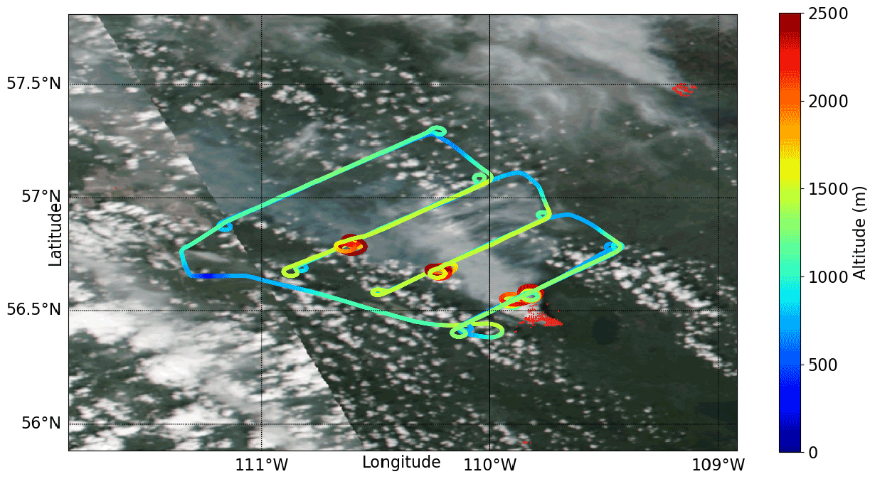
Figure 1 The aircraft flight tracks for the flight on 25 June 2018 during ECCC's aircraft campaign over the AOSR are shown. The colour indicates the altitude of the aircraft. The overlay is a VIIRS true-colour image together with the MODIS fire hotspots, shown as red dots (obtained from NASA Worldview; https://worldview.earthdata.nasa.gov/, last access: 19 July 2021).

Here, measurements from three flights that characterize two different fires are used; these three flights have good overlap with the TROPOMI overpass time (within approximately ±30 min). The Rabbit Foot Fire was measured on 12 August (RF11) and 15 August (RF13) 2018 and originated in Idaho, US, located at approximately 44.83^∘ N, 114.31^∘ W. The Watson Creek Fire burned in Oregon, US, at approximately 42.6^∘ N and 120.8^∘ W and was measured on 25 August 2018 (RF21). Further details, including the flight path, are presented in Sect. 5.3 (Fig. 10).

2.3.3 WE-CAN

The WE-CAN campaign, coordinated with the BB-FLUX campaign, also took place in the summer of 2018 in the northwestern US (based in Boise, Idaho), in many cases covering the same fires as the BB-FLUX campaign (Lindaas et al., 2021). The NCAR/NSF C-130 research aircraft was equipped with numerous instruments, including a NO_yO₃ chemiluminescence instrument, which measured the NO and NO₂ concentrations at 1 Hz. The uncertainties are 6 % for NO and 12 % for NO₂ for concentrations >1 pptv. Further details about the campaign and the measurements can be found in Lindaas et al. (2021), Juncosa Calahorrano et al. (2021), and Peng et al. (2020). Data are publicly available from https://www-air.larc.nasa.gov/cgi-bin/ArcView/firexaq?MERGE=1 (last access: 19 July 2021).

2.3.4 FIREX-AQ

The FIREX-AQ campaign (Wiggins et al., 2020; https://csl.noaa.gov/projects/firex-aq/, last access: 10 December 2021​​​​​​​) sampled western US wildfires aboard the NASA Douglas DC-8 research aircraft from July to August 2019. Smoke plumes were sampled with a comprehensive suite of instrumentation that measured both gas- and particle-phase species and optical properties. NO and NO₂ measurements were taken with a chemiluminescence instrument, and the on-board NASA Langley airborne High Spectral Resolution Lidar (HSRL) (Zhou et al., 2021) measurements of aerosol extinction at 532 nm were used to calculate emissions for perpendicular plume transects as described below. The NO_yO₃ chemiluminescence instrument uses the same detection technique as that used during WE-CAN, and NO and NO₂ associated uncertainties were ±(5 % + 6 pptv) and ±(7 % + 20 pptv), respectively (Ryerson et al., 2000; Pollack et al., 2010).

Total carbon fluxes were estimated for each aircraft plume crossing using methods outlined in Stockwell et al. (2021). Briefly, vertical lidar aerosol extinction profiles measured aboard were scaled to total carbon using all on-board measurements of carbon-containing compounds and in situ aerosol extinction. The total carbon emission rate (g/s) was estimated by calculating a carbon flux through each pixel area, applying average wind speeds measured at several altitudes, and then integrating through the height and width of the plume. Carbon emissions were then scaled to a mass emission rate of NO and NO₂ using transect-derived enhancement ratios of NO or NO₂ to total carbon. These ratios (specific for each transect) are applied to the carbon emissions to obtain NO and NO₂ emissions; the final NO_x emissions are the sum of the NO and NO₂ emissions. The total measurement uncertainty ranged from ∼20 %–60 % by fire. In total the emissions from five different flights were within 1 h prior to the TROPOMI satellite overpass: the North Hills Fire on 26 July 2019 (46.75^∘ N, 111.92^∘ W; Montana, US); the Williams Flats Fire on 3, 6, and 7 August 2019 (47.94^∘ N, 118.62^∘ W; Washington, US); and the Castle Fire on 12 August 2019 (36.53^∘ N, 112.23^∘ W; Arizona, US). Further details, including the flight path, are presented in Sect. 5.2 (Fig. 9). Data from FIREX-AQ are publicly available and can be downloaded from https://asdc.larc.nasa.gov/project/FIREX-AQ (last access: 19 July 2021; DOI: https://doi.org/10.5067/SUBORBITAL/FIREXAQ2019/DATA001, NASA, 2019).

3 Methodology

3.1 AMF with explicit aerosol correction

Fire plumes contain significant amounts of aerosols that scatter the UV–vis light and, thus, have a significant impact on the AMF. The standard TROPOMI NO₂ product does not consider aerosols but has an implicit aerosol correction by assuming that smoke plumes are clouds. Note that smoke and clouds are distinguished by the satellite-derived cloud fraction. This can introduce additional uncertainties in fire emission estimates impacted by smoke plumes. Liu et al. (2020) found that over urban areas the implicit aerosol correction might lead to underestimated NO₂ VCDs of up to 50 %. In this study, we use alternative AMFs to convert the TROPOMI SCD to a VCD and examine the impact on the TROPOMI tropospheric NO₂ columns near fire hotspots. This approach is very similar to previous studies focusing on the AMF estimate (McLinden et al., 2014; Griffin et al., 2019, 2020a), with the main difference in the accounting of aerosol scatter, in the form of aerosol optical depth (AOD). The tropospheric VCD is determined using the relationship VCD = SCD/AMF:

$$\begin{array}{}\text{(1)}& \begin{array}{rl}\mathrm{SCD}& =\sum _z\mathrm{nd}\left(z\right)\cdot \mathrm{bAMF}\left(z\right)=\mathrm{VCD}{\displaystyle \frac{{\sum }_z\mathrm{nd}\left(z\right)\cdot \mathrm{bAMF}\left(z\right)}{{\sum }_z\mathrm{nd}\left(z\right)}}\\ & =\mathrm{VCD}\cdot \mathrm{AMF},\end{array}\end{array}$$

where nd(z) is the NO₂ number density vertical profile (in units of mol/m³) along horizontal layers z, and bAMF(z) is the layer indexed AMF; and thus the total-column AMF is defined as

$$\begin{array}{}\text{(2)}& \mathrm{AMF}={\displaystyle \frac{{\sum }_z\mathrm{nd}\left(z\right)\cdot \mathrm{bAMF}\left(z\right)}{{\sum }_z\mathrm{nd}\left(z\right)}}.\end{array}$$

This is summed over altitudes between the surface and the tropopause. For the plume shape of NO₂ nd(z), we separate the satellite observations into areas inside and outside the fire plume. Here, we use 1 ×10¹⁵ molec/cm² (of the VCD_KNMI) as a threshold for enhanced columns; observations below this threshold are assumed to be outside the plume. To obtain a better understanding of the plume shape, we utilize the TROPOMI AER_LH product (aerosol_mid_height) and average the aerosol layer height observations over the entire plume. Note that there is typically not good enough coverage to use the aerosol layer height for each TROPOMI NO₂ pixel; thus, we use the average instead. Inside the plume we use a NO₂ a priori profile that is well mixed between the surface and the TROPOMI aerosol layer height rounded up to the closest 500 m (above ground), scaled by the standard KNMI VCDs (VCD_KNMI):

$$\begin{array}{}\text{(3)}& N\left(z\right)=n\left(z\right)\cdot ({\mathrm{VCD}}_{\mathrm{KNMI}}-{\mathrm{VCD}}_{\mathrm{above}}),\end{array}$$

where n(z) is the normalized profile shape, N(z) is the new a priori NO₂ profile used to estimated nd(z) (in Eq. 4), and VCD_above is the VCD contribution above the plume. Between the aerosol layer height (rounded up) and 12 km are background conditions, and we use the concentrations from a monthly GEOS-Chem model run at the approximate time of the TROPOMI overpass on a 0.5^∘ × 0.67^∘ resolution version v8-03-01 (http://www.geos-chem.org, last access: 10 December 2021​​​​​​​, Bey et al., 2001; McLinden et al., 2014). We use the GEOS-Chem profile, as the free-tropospheric NO₂ is not well represented in GEM-MACH due to missing elevated sources such as lightning and aircraft (Griffin et al., 2019). The NO₂ amount above the plume is on the order of 10¹⁴ molec/cm² and small compared to the total tropospheric column inside fire plumes (∼10¹⁵–10¹⁶ molec/cm²). However, it is better to assume even a small amount of NO₂ in the free troposphere when estimating AMFs than assuming 0. This a priori estimate is a simplification of the true profile shape; however, (Griffin et al., 2020b) showed that the TROPOMI aerosol layer height captures the main plume closer to the surface well, which is commonly well mixed. Prescribing specific profiles based on observations is not practical to estimate a smoke plume specific AMF in an operational manner.

The AMF(z) is the altitude-dependent AMF and is specific to each scene. Here, the SASKTRAN radiative transfer model (Bourassa et al., 2008; Zawada et al., 2015; Dueck et al., 2017) has been used to generate an altitude-dependent AMF lookup table (LUT) for clear sky (and cloudy conditions), as a function of solar zenith angle, viewing zenith angle, relative azimuth angle, surface pressure, surface albedo (cloud pressure), AOD (for several values between 0 and 3), and top-of-the-aerosol-layer height (between 0 and 4 km). For simplicity, the aerosol profile is assumed to be well mixed between the surface and the TROPOMI aerosol layer height (rounded up) and is 0 above. This is a simplification of the aerosol profile shape; however, this shape is a good approximation of the bulk of the plume (if the plume is not elevated) (Griffin et al., 2020b) and is computationally cheaper for the LUT estimate. For the LUT a log-normal aerosol size distribution is assumed with r=0.1 µm, σ=0.3, and a refractive index of 1.5+0.1i at 440 nm (Kou, 1996). Ozone (O₃) is not considered as it is not important in the wavelength range used for the NO₂ retrieval (van Geffen et al., 2018). Two different AMFs are estimated from the LUT: one for clear sky (AMF_cs) and one for cloudy sky (AMF_cd). The final AMF is estimated by using the cloud radiance fraction, cf (from original TROPOMI file):

$$\begin{array}{}\text{(4)}& \mathrm{AMF}=\mathrm{cf}\cdot {\mathrm{AMF}}_{\mathrm{cd}}+(\mathrm{1}-\mathrm{cf})\cdot {\mathrm{AMF}}_{\mathrm{cs}}.\end{array}$$

The cloud and clear-sky AMFs are only considered outside the plume for the following reason: the cloud fraction has contributions from clouds and aerosols and cannot be entangled. Inside the plume, the aerosols are already accounted for; thus, if clouds were considered again, these smoke aerosols would be accounted for twice, explicitly and implicitly (as smoke is mistaken for clouds). So while assuming no clouds (inside the smoke plume) might underestimate the impact of clouds if there are clouds in addition to the smoke aerosols, assuming clouds (in addition to the aerosols) will definitely overestimate the effect of clouds for all cases. Additionally, if clouds and smoke aerosols overlap, the cloud fraction is more likely to be above 0.5 and will be consequently filtered. As such, inside the smoke plume (with the VCD${}_{\mathrm{KMNI}}>\mathrm{1}\times {\mathrm{10}}^{\mathrm{15}}$ molec/cm²) we assume clear sky (cf=0) and only correct for the smoke aerosols without the additional clouds. Considering the cloud fraction in addition to aerosols will lead to an increase in the NO₂ VCD (Fig. 2f) that is considered as part of the AMF uncertainty. Outside the smoke plume, the cloud fraction is taken into account, as done in the original TROPOMI AMFs, and for the cloudy-sky AMF (AMF_cd), the cloud input is taken from the original TROPOMI files (cloud_fraction_crb_nitrogendioxide_window and cloud_pressure_crb).

We use the AOD retrieved from the Visible Infrared Imaging Radiometer Suite (VIIRS) aboard S-NPP at 445 nm (VAOOO) at 6 km resolution (publicly available from https://www.avl.class.noaa.gov, last access: 10 December 2021,​​​​​​​ Jackson et al., 2013), which is similar to the TROPOMI pixel size and the wavelength that is used to derive NO₂ (440 nm). The overpass time of S-NPP is similar to that of TROPOMI, within a few minutes. An example of the VIIRS AOD for the Williams Flats Fire on 7 August 2019 is shown in Fig. 2b.

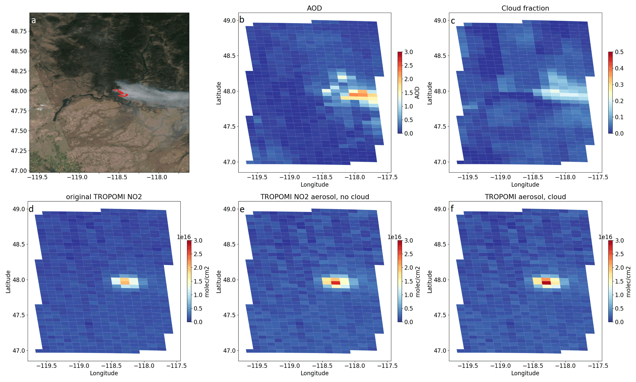
Figure 2 Williams Flats Fire on 7 August 2019 (also measured during the FIREX-AQ campaign). Panel (a) shows the VIIRS true-colour image together with the MODIS fire hotspots (obtained from NASA Worldview; https://worldview.earthdata.nasa.gov/, last access: 10 December 2021​​​​​​​). Panel (b) shows the VIIRS AOD at 445 nm mapped on the TROPOMI pixels. The cloud fraction is displayed in panel (c). The tropospheric NO₂ VCD_KNMI values are displayed in panel (d) and the VCD_EC values in panel (e) and (f), without and with accounting for clouds.

Following the approach from Griffin et al. (2019), the surface pressure input is taken from the operational GEM weather forecast model, interpolated to the location and time of the TROPOMI overpass. To improve the albedo spatial resolution, we use the MODIS albedo at a resolution of 0.05×0.05^∘ (collection 6.1 MCD43C3; Schaaf et al., 2002). A monthly-mean albedo is computed from the MCD43C3 files considering only 100 % snow-free pixels; snow-covered pixels are not a concern in this study, as there are no snow-covered areas near forest fires.

Outside of the plume we use the NO₂ profile from GEOS-Chem (representing background concentrations) and use the cloud fraction to determine the contribution between the cloudy- and clear-sky AMF. The KNMI and EC VCDs are compared in Sect. 5.1. For the VCDs outside of the plume, we found that there is very little difference between the two versions.

An example of the NO₂ tropospheric VCDs, with and without an explicit aerosol correction, is shown in Fig. 2 for the Williams Flats Fire on 7 August 2019. Figure 2a displays the VIIRS true-colour image at approximately the same time as the TROPOMI overpass together with the MODIS thermal anomalies (red dots), showing no clouds over the fire plume. Figure 2b shows the VIIRS AOD. The cloud fraction can be seen in panel (c), showing that the smoke plume is identified as clouds. The NO₂ VCD_KNMI and VCD_EC are shown in panels (d) and (e), respectively. This illustrates that the NO₂ VCD can change significantly when the AOD is accounted for; in this example, the NO₂ VCDs increase over the fire hotspot. Note that the explicit aerosol correction can increase or decrease the VCDs; the relationship is not a simple linear relationship but instead depends on the viewing geometry and AOD (see Fig. D1 in Appendix D for more details). In this example, accounting for clouds in addition to the smoke aerosols is probably incorrect, as there were no clouds mixed with smoke. Figure 2f shows the VCDs if both the aerosols and cloud fraction are considered in the estimate: this increases the NO₂ VCD (in this case, again this can go either way depending on the viewing geometry and AOD) in comparison to assuming no clouds, as in Fig. 2e. Panel (f) is only shown for comparison purposes; this approach accounts for smoke aerosols twice, explicitly and implicitly, and is therefore not recommended. Outside fire plumes, where the NO₂ is at background levels, as expected, the VCD_KNMI and VCD_EC are very similar.

3.2 Methods for estimating emissions from satellite data

Satellite observations provide information on the total amount of a trace gas released from a source; however, additional information on transport and chemical processes is required to estimate emission rates. An important component that enables the estimation of emissions from satellite observations is information on wind direction and wind speed.

In a first step, the satellite observations are rotated to obtain an upwind–downwind domain near the emission source using the wind fields at the time and location of the observations (e.g. Pommier et al., 2013; Fioletov et al., 2015; Dammers et al., 2019). Here, we utilize the wind fields (U, V) from the European Centre for Medium-Range Weather Forecasts (ECMWF) ERA5 dataset at a resolution of $\mathrm{0.25}{}^{\circ }\times \mathrm{0.25}{}^{\circ }$ with an hourly output between 1000 and 300 hPa at a resolution of 50 hPa. Note that the observations are rotated around a single point, which will cause some imperfections for large fires that are not true point sources as they are spread over larger areas.

As fire emissions can be injected into higher altitudes, wind speeds and wind directions can vary significantly at different altitudes. Griffin et al. (2020b) found that TROPOMI plume heights are a good proxy for the average height of the fire plumes. Here, we use the average TROPOMI aerosol layer heights (AER_LH) for each individual fire and use this to obtain the corresponding wind direction and speed and average the wind fields within ±50 hPa for the corresponding plume height. In cases where no good-quality plume heights were found, we use the average plume height of fires, 2 km (or 800 hPa) (Griffin et al., 2020b). The wind fields are linearly interpolated to the time of the satellite overpass.

There are multiple ways to estimate emissions from satellite observations. Here, we compare two common direct estimation methods that are best suited to estimate daily fire emissions from TROPOMI: (1) a flux method that has previously been used to estimate fire emissions from OMI (Mebust et al., 2011; Adams et al., 2019) and for CH₄ emission estimates using GHGSat and TROPOMI (Varon et al., 2018, 2019) and (2) a 2-D exponentially modified Gaussian (EMG) method (e.g. Fioletov et al., 2015; Dammers et al., 2019). A study by Jin et al. (2021) recently reported TROPOMI-derived NO_x emissions using a 1-D EMG method, fitting the plume in an across-wind direction.

3.2.1 Flux method

The flux method, also know as integrated mass enhancement method, is similar to the method used by Mebust et al. (2011), Adams et al. (2019), and Varon et al. (2019): wind-rotated VCDs are integrated to find the total mass inside a box and account for the total mass that has entered the box. As a first step, the background is subtracted from the VCDs; this is an important step that can influence the emission rate significantly based on the methods chosen. We investigated various ways to subtract the background: (1) 10th percentile in the surrounding area within 100 km distance from the fire, (2) fitted background, and (3) within 25 to 50 km upwind of the fire. Based on tests with model VCDs (see Sect. 4.2, we chose to define the background based on the average upwind concentrations (method 3). Next, the VCDs are rotated around the centre of the fire, and the wind-rotated VCDs are gridded using the satellite footprint. The VCDs are then integrated inside boxes that are 4 km long (upwind/downwind direction) and 50 km wide (perpendicular to the wind direction) and multiplied by the wind speed to find E_y, the flux (in g/s) y km downwind of the fire. The initial emissions at the source (described in detail in Mebust et al., 2011) are found by

$$\begin{array}{}\text{(5)}& E=E_y\cdot {\displaystyle \frac{t_c}{\mathit{\tau }\cdot (\mathrm{1}-\exp (\frac{t_c}{\mathit{\tau }}\left)\right)}}.\end{array}$$

$t_c=x_c/u$ is the residence time inside the box of a width x_c and wind speed u, and τ is the lifetime or e-folding time. This method is very sensitive to the wind speed as it directly impacts the emission rate. The final emission rate obtained using this method is an average of all emission rates within 20 km downwind of the fire centre. An example is shown in Fig. 3 for the Watson Creek Fire (also observed by the BB-FLUX campaign) on 25 August 2018 at approximately 43.5^∘ N, 120.7^∘ W in Oregon, US. Panel (a) shows the raw NO₂ VCD as observed by the satellite with the fire hotspot in the middle. Panel (b) shows the wind-rotated and smoothed VCDs (background subtracted); here, the red lines show the area of the 4×50 km² boxes used for the estimate of the emission flux. The emissions (following Eq. 5) for each box are shown in panel (c). To obtain the final number for the emissions only the boxes within 20 km of the fire are averaged (Adams et al., 2019), which ensures that the entire fire is captured and enough TROPOMI observations are used for the estimate. Limiting the estimate to within 20 km of the fire reduces the impact of the diurnal variability of the fire emissions; on average the NO_x molecules within 20 km were emitted roughly within 1 h of the TROPOMI overpass. It also ensures that the first box, near the fire hotspot, is larger to make sure that the entire fire area, which might be a few kilometres upwind of the fire centre, is captured. Further than 20 km downwind of the fire, the uncorrected emission rate (black stars) drops due to the short lifetime (including chemistry, deposition, and dispersion) of NO₂. The colours in Fig. 3c indicate the different assumed lifetimes (τ) for NO₂, 1 h (red), 2 h (green), 4 h (blue), and 6 h (purple), and no correction of the lifetime (equivalent to infinite lifetime; black stars). The differences in the inferred emissions for different NO₂ lifetimes (τ) are relatively small if the lifetime is longer than 3 h; however, the impact on the retrieved emissions increases rapidly as τ falls below 2 h.

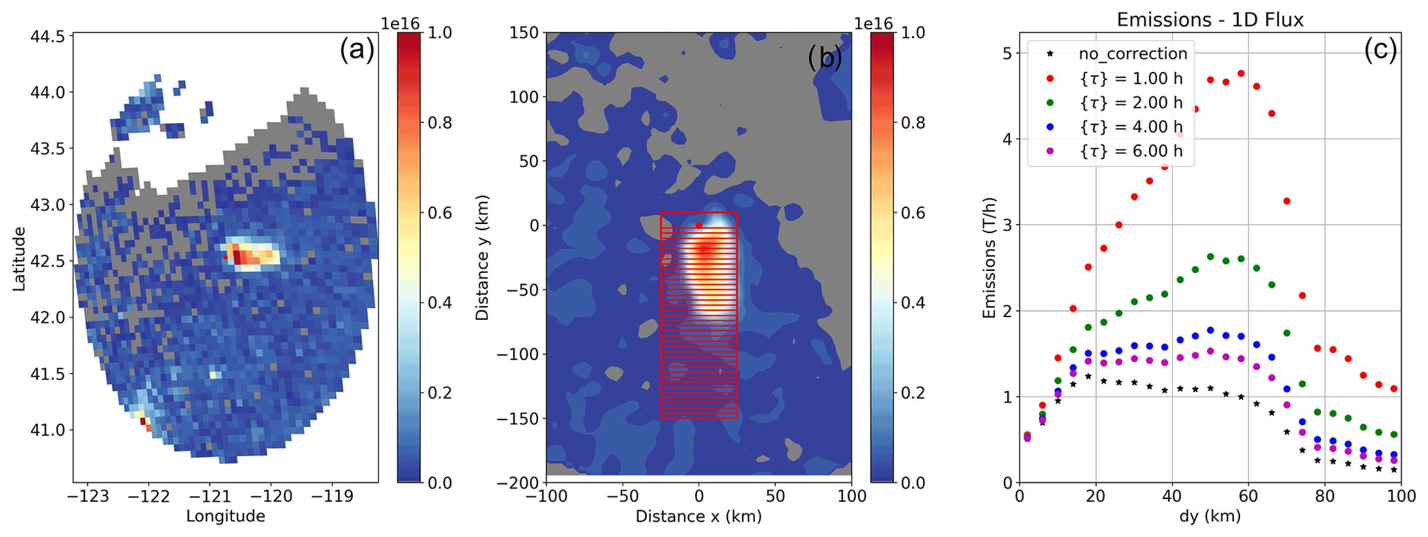
Figure 3 Example of the flux fit for the Watson Creek Fire on 25 August 2018 at approximately 43.5^∘ N, 120.7^∘ W in Oregon, US. The TROPOMI observations (VCD_EC) are shown in panel (a) in a latitude–longitude domain with the fire centre in the middle (shown as a red dot). The background is subtracted from the VCDs and then rotated (along the wind direction) and smoothed (weighted by the footprint coverage), shown in panel (b) in an upwind–downwind domain (in km) with the fire at its centre. The mass is summed inside the 50 × 4 km² (shown as red boxes), and using Eq. (5) the emission rate is estimated for each of the boxes assuming a variety of lifetimes for NO₂, shown in panel (c).

3.2.2 Exponentially modified Gaussian

While the flux method simply sums up all mass emitted by the fire, emissions can also be estimated by fitting a Gaussian plume to the observations. To describe the distribution of the NO₂ VCD field near the source, an exponentially modified Gaussian (EMG) function can be used (see Eqs. A1–A4 in the Appendix). Using a Levenberg–Marquardt algorithm the enhancement factor a is derived by minimizing the difference between the fitted and observed VCDs. The enhancement factor is directly linked to the emissions E by

$$\begin{array}{}\text{(6)}& E={\displaystyle \frac{a}{\mathit{\tau }}}.\end{array}$$

The EMG method has previously been applied to estimate SO₂ (Fioletov et al., 2015; McLinden et al., 2020) and NH₃ (Dammers et al., 2019) emissions from satellite observations. Here, contrary to the previous studies that used many days or even years to estimate the emissions, the observations are not gridded by different wind speeds as only single days are fitted. After applying a wind rotation to the tropospheric VCDs, the EMG was used to estimate the emissions from a point source. The lifetime ($\mathit{\tau }=\mathrm{1}/\mathit{\lambda }$) and the plume spread (σ) can be estimated at the same time; however, there are many solutions for λ and σ. Therefore, to avoid overfitting the parameters due to the limited amount of observations for single days, λ and σ were kept constant. Natural variations of λ and σ are later accounted for in the uncertainty estimate.

An example of the method is shown for the Watson Creek Fire on 25 August 2018 in Oregon, US. Figure 4a and b show the satellite observations in a longitude–latitude domain and in a wind-rotated upwind–downwind domain, respectively. The lower panels (c) and (d) show the fitted VCDs (after the EMG has been applied) in the longitude–latitude domain and the upwind–downwind domain, respectively.

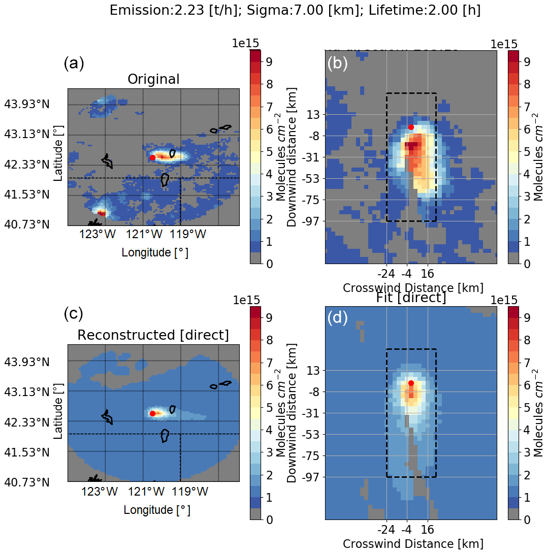
Figure 4 Example of the EMG method for the Watson Creek Fire on 25 August 2018 at approximately 43.5^∘ N, 120.7^∘ W in Oregon, US (same as in Fig. 3). The TROPOMI NO₂ observations (VCD_EC) are shown in a latitude–longitude and upwind–downwind domain in panels (a) and (b), respectively. The fitted VCDs using the EMG are shown in panels (c) and (d) in the longitude–latitude and upwind–downwind domain, respectively.

4 Accuracy of the emission estimates using synthetic data

To determine the accuracy of the emission estimates, we use synthetic NO₂ and NO VCDs with prescribed emissions and test if these emissions can be determined with the flux and EMG methods, as described in the previous section. The GEM-MACH air quality model was used to obtain the synthetic VCDs. Here, we use a special model run, where the emissions from various fire hotspots are held constant for a 24 h period to remove any diurnal variability. This is needed in order to simplify the sensitivity study and to determine if the methods can accurately reproduce the input emissions, as any diurnal variability will impact the VCDs over time (downwind) and, thus, complicate the analysis. The model NO₂ and NO profiles are integrated over the first 39 layers (approximately 10 km) to obtain VCDs; the NO_x VCDs are the sum of the NO₂ and NO VCDs. NO₂ VCDs cannot be directly compared to NO₂ input emissions due to the GEM-MACH model chemistry and oxidation from NO to NO₂. Thus, we use NO_x VCDs and compare those to the NO_x model input emissions (ENO + ENO₂). In the model approximately 90 % of NO_x is emitted as NO and converts to NO₂ (based on the reaction mechanism within the model). In this section sensitivity tests are performed testing the flux and EMG methods using model NO_x VCDs and known emissions. Since TROPOMI can only measure NO₂, the scaling from NO₂ to NO_x is important for the emission estimate and discussed in the following section.

4.1 Lifetime and plume spread

The NO₂ lifetime (or decay time) and plume spread (or dilution) can be determined with the EMG method (see Eqs. A1–A4). However, based on our analysis, using just single overpasses, these only return reasonable results of the lifetime and plume spread for less than 30 % of fires. Thus, for this study we kept the lifetime and plume spread the same for each fire. A variety of fires were used to determine a suitable lifetime and plume spread using the EMG method. Based on good EMG fits for various fires, we obtained a mean lifetime of 1 h (±0.5 h) for NO_x and a plume spread of 6 km (±1 km) when the model VCDs are used. When applying the EMG method to TROPOMI observations, we derived a mean lifetime of 2 h (±1 h) for NO₂ and a plume spread of 7 km (±1 km). Note that the difference of the lifetime between the model and the TROPOMI observations is expected, since the chemical lifetime of NO₂ is shorter in the model compared to reality (it can be seen in the fire plumes that dissipate faster in the model compared to the satellite observations). The lifetime derived from the EMG is not a true chemical lifetime but is also influenced by plume dispersion and surface deposition as described by de Foy et al. (2015). Juncosa Calahorrano et al. (2021) found an average NO_x lifetime or e-folding time of 90 min inside fire plumes using aircraft measurements during the WE-CAN campaign. Our satellite-derived lifetime of 2 h (±1 h) using the EMG method agrees with their results within the uncertainties. The plume spread parameter incorporates several effects, including the diffusion of the plume in the crosswind direction, the spatial extent of the source, and the size of the satellite pixel. The plume spread parameter is only used for the EMG method, and the flux method does not take this into account. Note that for the EMG, changes in lifetime and plume spread can compensate for each other: a shorter lifetime will increase the emissions and a smaller plume spread will decrease the emissions. Thus, the emissions are almost identical (within 5 %–10 %) when using for example σ=7 km and τ=1.5 h, as well as σ=6 km and τ=1 h.

For the estimates in this section, when using the model VCDs, we apply a constant plume spread and lifetime of 6 km and 1 h. When utilizing the TROPOMI observation (in Sect. 5), we set the lifetime for both the EMG and flux method to $\mathit{\tau }=\mathrm{2}(\pm \mathrm{1})$ h.

4.2 Reproducing the synthetic emissions

In this section, four sensitivity tests are performed testing the flux and EMG method (as described in Sect. 3.2.1 and 3.2.2): (i) using the model sampling and model winds (best-case scenario), (ii) using satellite sampling, (iii) using satellite sampling and ERA winds (different winds than the winds used in the GEM-MACH model), and (iv) using satellite sampling and ERA winds, as well as adding a random error similar to that of the TROPOMI observations (scenario closest to using satellite observations). The results from the sensitivity test are shown in Fig. C1 for the flux method and EMG method, respectively. In total the emissions of over 59 fires (in North America) for the month of June 2018 were successfully retrieved and subsequently compared. Two fires had unusual wind conditions, with very high winds and wind shear that have been excluded from the analysis. Scenario (i) is shown in panel (a), scenario (ii) in panel (b), scenario (iii) in panel (c), and scenario (iv) in panel (d).

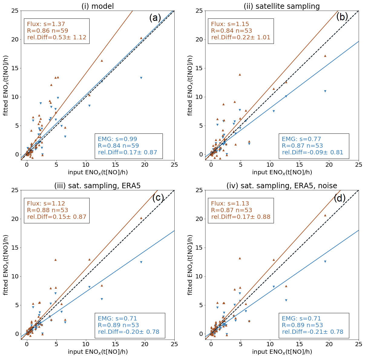
Figure 5 The results of the sensitivity test with synthetic data for test (i)–(iv) are illustrated (see text for detailed description of the scenarios). The fitted emissions applying the flux (orange triangles) method and the EMG method (blue downward triangles) versus the model input emissions are plotted together with the statistics (slope of best fit using the geometric mean, s; correlation coefficient, R; the number of points, n; and the mean and standard deviation of the relative difference, rel. Diff: input − fitted).

For scenario (i) the emissions are highly correlated to the input emissions with R>0.8 for both the flux method and the EMG. The fitted emissions are biased high by about 37 % (based on the slope) using the flux method. The EMG is more accurate for this scenario and has no bias with a line of best fit close to the 1:1 line.

Scenario (ii) assumes satellite sampling (the synthetic observations are filtered when the real TROPOMI quality flags are less than 0.5); thus, the number of observations for the fit will be less, especially close to fire where observations are removed by the cloud filter due to the high smoke content. The impact of this on the emission estimate is shown in panel (b) in Fig. C1. This impacts the number of fires that can be retrieved: reduced to 53 fires – roughly 10 % fewer successful fire retrievals can be expected, which is the case for both methods. Furthermore, using the satellite sampling leads to, on average, lower emissions: the flux method, based on the slope, is still biased high by about 15 %, and the EMG is now biased low by about 23 % (the relative difference is about 10 %) compared to the true synthetic emissions. The correlation coefficient is slightly smaller but still shows a correlation with R∼0.9 for both methods.

In scenario (iii), see panel (c) in Fig. C1, in addition to the satellite sampling, the winds were changed to the wind fields from ERA5, which can be different than the wind fields of the model. Since in reality the true winds are unknown and likely differ to some extent from the ERA5 winds, this scenario is a more realistic scenario compared to the two previous ones. This has little impact on the slope and correlation.

The measured VCDs are not perfect and have some instrument noise. In the previous tests, perfect model VCDs were used, whereas in this last scenario (iv), a random error has been applied to the model VCDs. A random error of 0.7 ×10¹⁵ molec/cm² was applied to the model VCDs and is similar to the reported noise of the TROPOMI observations. Adding a random error has a minimal effect on either the flux or EMG method; see panel (d) in Fig. C1. On the other hand, if there is a bias in the satellite VCDs, that will affect the emission estimate; this can, however, be corrected with recalculated AMFs and high-resolution input data.

While the slope is closer to the 1:1 line for the flux method compared to the EMG method, for scenario (ii)–(iv), there is less scatter and more consistency for the EMG method especially for emissions less than 5 t[NO]/h (which is the range of the emissions compared in Sect. 5). For instance, for emissions less than 5 t[NO]/h, for scenario (iv), the EMG has a relative difference of −3 % and a slope of 1.24, whereas the flux method has a relative difference of −42 % and a slope of 1.94.

4.3 NO₂-to-NO_x scaling

The chemistry of NO_x is complex, including a fast inter-conversion between primary emissions of NO and secondary NO₂. Current satellites, such as TROPOMI, can only measure NO₂. Thus, the scaling factor from NO₂ to NO_x is important. Only a limited number of studies investigate this scaling for satellite-derived NO_x emissions from NO₂ observations (e.g. Adams et al., 2019; Lorente et al., 2019). Here, we use the synthetic data and derive NO_x emissions from NO_x VCDs and compare these to NO₂ emissions from NO₂ VCDs by applying the EMG to those VCDs. This can help to understand how the satellite-derived NO₂ emissions can be scaled to NO_x emissions and if this is even possible; i.e. a large scatter of NO_x (from NO_x VCDs) and NO₂ (from NO₂ VCDs) derived emissions would indicate that the conversion is not stable and NO_x emissions could not be derived from NO₂ VCDs without further information of other parameters. The results are shown in Fig. 6, where there is a perfect correlation (R=1) between the fitted NO₂ and NO_x emissions that are based on the model VCDs for 59 different fires across North America. While the NO_x input emissions are emitted as 90 % NO and 10 % NO₂ for all fires, the conversion and lifetime can change based on the different OH, NO_x concentrations, and temperature. Note that for this fit, all VCDs between 25 km upwind and 100 km downwind are used where the NO₂:NO_x ratio is changing with plume age. The derived ratio of 0.68, which allows us to convert the derived NO₂ emissions (from NO₂ VCDs) to total NO_x emissions, has a perfect correlation indicating that the scaling from derived NO₂ emissions to the net NO_x emissions is stable. This derived ratio has been applied to the TROPOMI-derived NO₂ emissions in this study to convert these to total NO_x emissions. Note that the model VCDs used for this analysis are from 20:00 UTC, close to the TROPOMI overpass time; a different ratio is likely for other times of day. We note that the emissions of NO_x will largely be in the form of NO: our NO₂-to-NO_x ratios above serve to convert our measured quantity, a satellite-derived emission of NO₂, to the net quantity relevant for emissions inventories and modelling, the total emissions of NO_x. The ratio described here is intended as a correction to return the net emissions of NO_x and should not be interpreted as the ratio of NO₂ to NO_x during the actual emissions process itself.

Figure 6 Fitted emissions derived using the EMG method for the synthetic NO₂ and NO_x (NO₂ + NO) VCDs, suggesting a NO₂:NO_x ratio of 0.68 should be used for the conversion; the fitted NO₂ and NO_x emissions are perfectly correlated (R=1).

To further support the NO₂:NO_x scaling, we also looked at aircraft measurements taken during ECCC's aircraft campaign over the AOSR (described in Sect. 2.3.1) on 25 June 2018 in Saskatchewan, Canada, and compared those to the model output for the same fire. The aircraft measurements were taken from near the surface to the top of the fire plume, at four downwind cross-plume transects at distances of approximately 20 to 100 km from the wildfire. The NO₂:NO_x concentration ratios were found from correlation of the scatter plots; the slope and the slope error (as error bars) from the aircraft measurements are shown in Fig. 7b; for comparison, the model NO₂:NO_x ratios for that fire are shown in Fig. 7a. The NO₂:NO_x slopes from the aircraft measurements have very high correlations for all four flight transects with R²>0.8 (R²=0.96, R²=0.9, R²=0.86, and R²=0.81 for transect 1, 2, 3, and 4, respectively). Near the fire the ratio is 0.71(±0.03) and is consistent with the model-derived ratio, as shown in Fig. 6. Downwind of the fire the ratio increases as more NO is oxidized to NO₂; this can be seen in the model results as well. The model NO₂:NO_x has the same intercept as the measured ratio; only the slope is lower, indicating the NO does not oxidize to NO₂ fast enough in the model; this leads to a lower NO₂:NO_x ratio further downwind (Fig. 7). It should be noted that for the EMG and thus the conversion from NO₂ to NO_x emissions, the VCDs close to the hotspot (roughly within 20 km from the fire) are driving the emission estimate. The ratio further downwind does not significantly impact the emission estimate, even though at 100 km downwind almost all measured NO_x is NO₂, because these VCDs are not driving the emission estimate and this ratio is not significant for the NO₂-to-NO_x scaling of the satellite-derived emissions. Close to the fire (within 20 km of the centre) the aircraft observations show a NO₂:NO_x ratio of 0.71–0.75. This analysis shows that the derived NO₂ emissions can be scaled to NO_x emissions and that this conversion is not the most significant source of uncertainty. It should be noted that this might be different for mountainous areas or large fires where the plume is lifted into the free troposphere, but for the fires investigated in this study the ratio to convert satellite-derived NO₂ emissions to NO_x emissions is stable. The model output is in good agreement with the aircraft observation, which shows a similar NO₂:NO_x ratio close to the fire. For studies looking to convert satellite-derived NO₂ emissions to NO_x emissions, based on this analysis, we recommend using a value between 0.68–0.75 for daytime satellite-derived NO₂ emissions (for early afternoon overpasses) and, thus, applying a factor of 1.3 ($=\mathrm{1}/\mathrm{0.75}$) to 1.5 ($=\mathrm{1}/\mathrm{0.68}$) to the satellite-derived NO₂ emissions to obtain the net NO_x emissions. For this study, we use a ratio of $\mathrm{1}/\mathrm{0.68}$ for the scaling from NO₂ to NO_x emissions. We also conducted further tests by converting TROPOMI NO₂ VCDs to NO_x VCDs, using a different ratio inside and outside the plume, to then determine the NO_x emissions. However, we found that this introduced more uncertainty and scatter in the emission estimate. Based on these tests, we recommend retrieving the NO₂ emissions from satellite NO₂ VCDs before converting the derived NO₂ emissions to NO_x emissions.

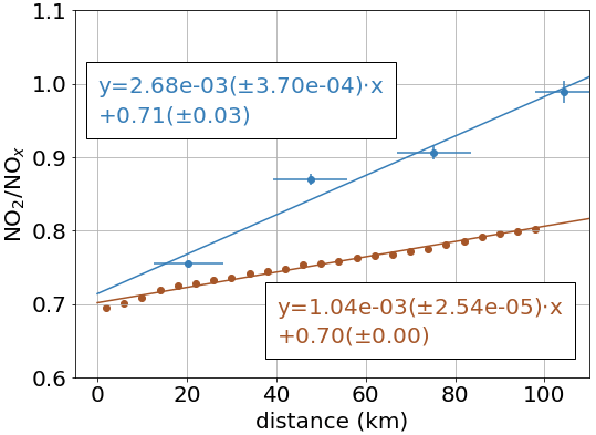
Figure 7 NO₂:NO_x ratio using model output (orange) and aircraft measurements (blue) for the Lac La Loche fire on 25 June 2018. The model ratio using the synthetic NO₂ and NO_x (NO₂ + NO) VCDs downwind of the fire is shown as orange dots. The NO₂:NO_x ratio using in situ aircraft measurements for the same fire is shown as blue dots. Four cross-plume transects were flown at various altitudes capturing the entire fire plume at different distance from the fire.

4.4 Total uncertainties of the NO_x emission estimate

Overall, we found that the EMG method can accurately reproduce the model emissions exactly under perfect conditions, i.e. for model sampling and model winds, scenario (i). The sampling of the satellite has very little impact on the emissions for the EMG method for typical fires, scenario (ii). The imperfect winds result in the largest uncertainty and lead to an overall low biased emission estimate. The added noise did not impact the results of the EMG method. The flux method cannot reproduce the input emissions as well under a perfect scenario and tends to overestimate the emissions. However, the bias is reduced for the imperfect scenarios, as these uncertainties, such as the satellite sampling and ERA5 winds, overall reduce the emission estimate. Also for the flux method, the satellite noise had little impact on the emission estimate. The satellite sampling leads to approximately 10 % less successfully derived emissions for both methods, which is mostly due to cloud cover or very thick fire smoke.

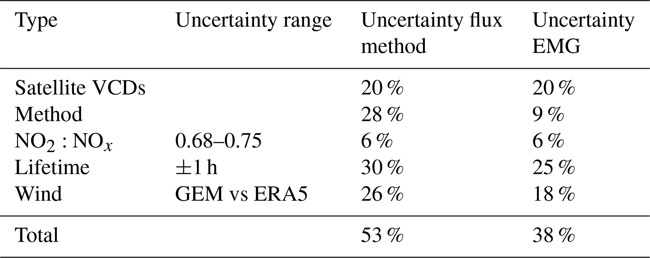
In order to estimate the total uncertainties for the satellite-derived emission estimates, we consider the following uncertainties: (1) the uncertainty from the method itself, (2) the uncertainties of the satellite VCDs or more specifically the AMFs, (3) the NO₂:NO_x conversion, (4) the NO_x lifetime, and (5) the uncertainty of the winds. A summary of uncertainties can be found in Table 1. For the method uncertainty, we use the relative difference of scenario (ii). The uncertainty due to the wind speed and plume height is based on the tests using different winds, where we use the relative difference between the emission estimates from scenario (ii) and (iii). The uncertainty of the wind speed also includes the uncertainty of the wind heights used to obtain the wind speed. The NO₂:NO_x uncertainty is based on the range of values we found for the conversion (0.68–0.75). The uncertainty due to lifetime is based on estimates using different lifetimes and plume spread ranges. The uncertainty of the satellite VCDs (20 %) is based on previous estimates of the AMF uncertainties (McLinden et al., 2014; Griffin et al., 2019), and a similar number was also obtained by comparing the new satellite VCDs to the aircraft VCDs in Sect. 5. The uncertainty of the satellite VCDs is really the uncertainty of the AMF which includes the uncertainties related to the assumptions and parameters used for the calculation of the AMF. To obtain the overall uncertainty, we added those uncertainties in quadrature. Note that this might overestimate the actual uncertainty as these components of the net uncertainty may have compensating effects leading to a better estimate; for example, the uncertainty of the winds leads to smaller emissions for the flux method which partially compensates for the overall high bias from the method.

Table 1 Summary of uncertainties for the satellite emission estimates.

Comparing the flux method to the EMG method, we found that the EMG method has higher correlation coefficients, less scatter for the NO_x emission estimates, and smaller total uncertainties. However, one of the primary disadvantages of the EMG method is the uncertainty in lifetime and plume spread. Thus, we would recommend a constant lifetime and plume spread when doing single day or overpass emission estimates with TROPOMI observations. It should also be noted that while the EMG successfully estimates the emissions for a short-lived species like NO_x, this method does not work as well for longer-lived species such as CO or CH₄, as these do not typically obtain a Gaussian plume shape as well (due to the long lifetime), except under very stable wind conditions. We would recommend using the flux method to obtain the emissions for those species.

5 Comparison to aircraft measurements

In Sect. 3.1, we described how new AMFs with an explicit aerosol correction were derived. Here, those newly estimated TROPOMI VCDs and TROPOMI-derived NO_x emissions are compared to aircraft-measured VCDs and aircraft-derived emissions. We compare (1) integrated VCDs utilizing measurements from the WE-CAN and FIREX-AQ campaign, similar to the previous work of Griffin et al. (2019), (2) NO_x emissions derived from airborne lidar and in situ carbon and nitrogen measurements from the FIREX-AQ campaign, and (3) TROPOMI VCDs and emission estimates to aircraft remote-sensing DOAS measurements taken during BB-FLUX campaign (following the approach from Theys et al., 2020).

5.1 Integrated profiles

To compare the aircraft measurements to the TROPOMI VCDs, the aircraft in situ measurements (flown as transects or spirals at various altitudes) are integrated to VCDs and averaged within the TROPOMI pixel, following the approach presented in Griffin et al. (2019); however, here we use a stricter coincident criterion of ±30 min of the TROPOMI overpass. This somewhat limits the number of measurements; however, fire emissions are highly variable, and thus relaxing the coincident criterion may affect the comparison. In total 41 TROPOMI observations are compared to the aircraft-measured VCDs from 12 different flights across two studies. An example profile is shown in Fig. 8c, where the black dots indicate the aircraft measurements and the red line is the interpolated profile used to estimate the aircraft VCD. To account for NO₂ measured above the aircraft, we include a monthly GEOS-Chem profile; however, this will account for very little of the total tropospheric VCD ($\sim \mathrm{1}\times {\mathrm{10}}^{\mathrm{14}}$ to 5×10¹⁴ molec/cm²). Below the aircraft we assume a constant volume mixing ratio (VMR) based on the measurements at the lowest aircraft altitude. The error bars shown in Fig. 8 indicate different profile extrapolation methods to the ground. On the lower end, an elevated plume is assumed and the VMR from the lowest altitude of the aircraft linearly decreases to 0 at the surface, and, on the upper end, twice as much NO₂ as the measurement of the lowest aircraft altitude is assumed near the surface.

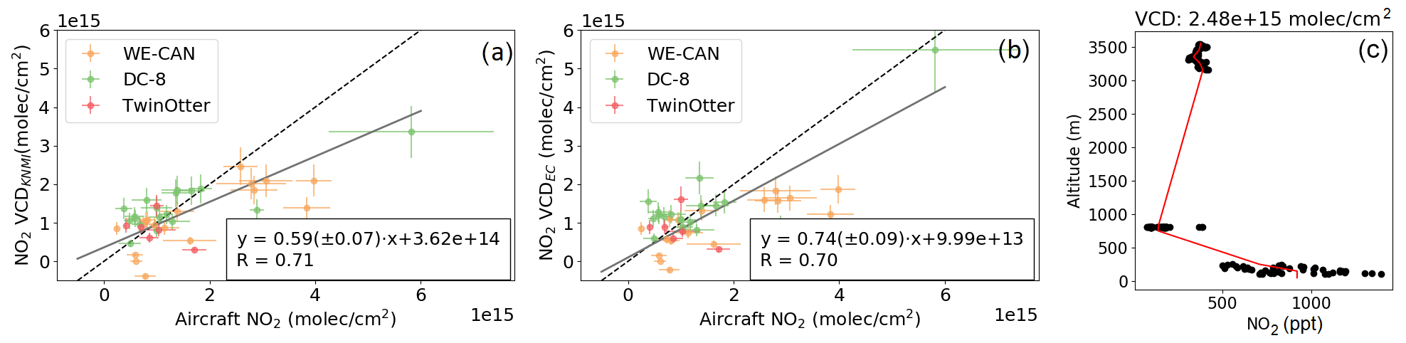
Figure 8 Comparison between aircraft measurements and TROPOMI NO₂ VCDs. Aircraft data were collected as part of the WE-CAN and FIREX-AQ (collected on the DC-8 and Twin Otter aircraft) campaigns in the western US in 2018 and 2019, respectively. The comparison is shown using (a) the VCD_KNMI and (b) the VCD_EC. An example aircraft profile is shown in panel (c), where the black dots indicate the aircraft measurements (WE-CAN campaign, RF08) and the red line is the interpolated profile used to estimate the aircraft VCDs.

Figure 8a and b show the comparison for the NO₂ VCD_KNMI and VCD_EC, respectively. Based on the correlation, the slope of best fit, and the mean difference between the aircraft and TROPOMI VCDs, the comparison suggests that the newly derived AMFs (VCD_EC) show an improvement over the original VCD_KNMI. Note that only a limited number of measurements are available, especially with high NO₂ VCDs. Thus, the slope and correlation are primarily driven by one high observation. An example of a profile (measured and interpolated) is shown in Fig. 8c: there are gaps in the measurements due to the stringent coincident criteria, and this comparison is not ideal. Thus, we included two further comparisons to aircraft-borne observations and aircraft-derived emissions in the following sections.

5.2 Emission comparisons

We compared the TROPOMI-derived emissions to aircraft-derived emissions from measurements taken during the FIREX-AQ campaign, as described in Sect. 5.2. To compare the satellite and aircraft-derived emissions, the time of the plume emission is estimated. For the aircraft emissions, the time of emission is based on the mean time, t_t, when the transect was flown (the transects typically take less than 5 min). We then assume the time of emission is t_t−τ for the aircraft-measured plume, where τ is the plume age. Plume ages were estimated by averaging HYSPLIT back trajectories from the aircraft position during the plume transect to the fire source using multiple meteorological datasets to account for spatial and temporal variations in the wind. Uncertainties are driven by errors in the meteorological datasets (wind variation), assumed vertical velocities, and inaccuracies in the fire source location. For the satellite observations the time of the emission is not as precise, as many measurements downwind of the fire are used for the estimate. For the flux estimate only measurements up to 20 km are used and averaged. For the EMG observations further downwind are used; however, as the magnitude of the NO₂ columns decreases downwind, they become less important for the overall magnitude of the enhancement a (see Eq. A1). Thus the most important observations are roughly within 20 km of the source (depending on the wind speed). The time of emissions for the satellite observations (based on average wind speeds) is an average of the hour prior to the satellite overpass. We define roughly the time of emissions for the satellite observations to be 30 ± 30 min prior to the satellite overpass. The time of emission from the satellite-derived emissions is a range of times, and a precise time cannot be determined, because the satellite NO₂ amounts that go into the emission estimate (downwind of the fire) were emitted at various times before the satellite overpass.

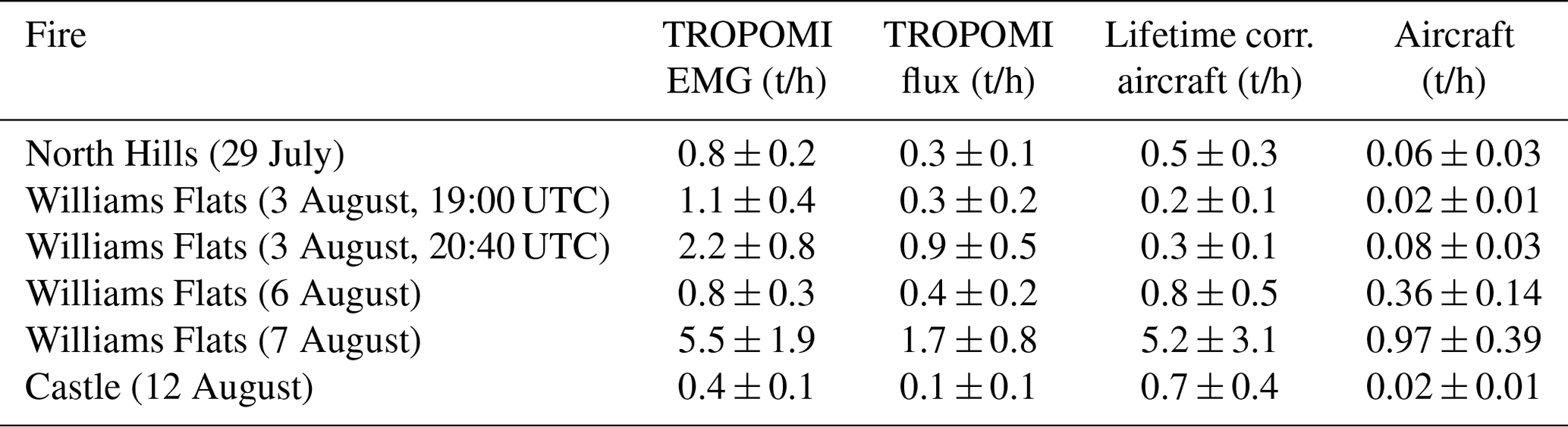
The comparison between the aircraft and the satellite-derived NO_x emission rates for the five overlapping flights is shown in Fig. 9 using the VCD_EC (and as a comparison the VCD_KNMI shown as crosses). The magnitude of total emissions from five different flights could be compared where the time of emission was within 1 h prior to the satellite overpass: the North Hills Fire, the Williams Flats Fire, and the Castle Fire. As NO_x has a short lifetime, the aircraft emissions were adjusted accordingly using the HYSPLIT estimated plume age (red triangles). A lifetime of 2 h (as was derived from the TROPOMI observations and EMG fits; see Sect. 4.1) was applied to the aircraft NO_x emissions (by multiplying a factor of $\mathrm{1}/\exp (-\text{plume age}/\text{lifetime})$) to determine the initial emission rate at the time of emission from the fire; for comparison, the original aircraft emissions are also shown (pink triangles). The fire radiative power (FRP) from the Geostationary Operational Environmental Satellite 17 (GOES-17) of these fires is shown in Fig. 9 as small grey dots as an indicator for diurnal fire intensity. GOES-17 is a geostationary satellite, also referred to as GOES-West, providing information such as FRP every 5–15 min primarily over the western part of North America (Li et al., 2020, and references therein). The aircraft-derived NO_x emissions follow the GOES-17 FRP well, with increased FRP tracking increased NO_x emissions. Six TROPOMI overpasses are coincident (shown as shaded grey areas in Fig. 9) with aircraft-derived emissions. The satellite- and aircraft-derived emissions are summarized in Table 2. The best agreement between the aircraft and satellite-derived emissions is found using the EMG method with the VCD_EC, for which the satellite and aircraft-derived emissions are within the estimated uncertainties, except for the Williams Flats Fire on 3 August, where the satellite-derived emissions are higher. For the first TROPOMI orbit on 3 August, the emissions are very low, and for the second orbit, the fire activity then increased rapidly, which is likely why there are discrepancies between the satellite- and aircraft-derived emissions that day as the emissions changed very rapidly during this time. The flux method always results in smaller emissions compared to the EMG and has a low bias compared to the aircraft-derived emissions. Using the VCD_KNMI for the estimate leads to smaller emissions for these fires which do not agree as well with the aircraft-derived emissions.

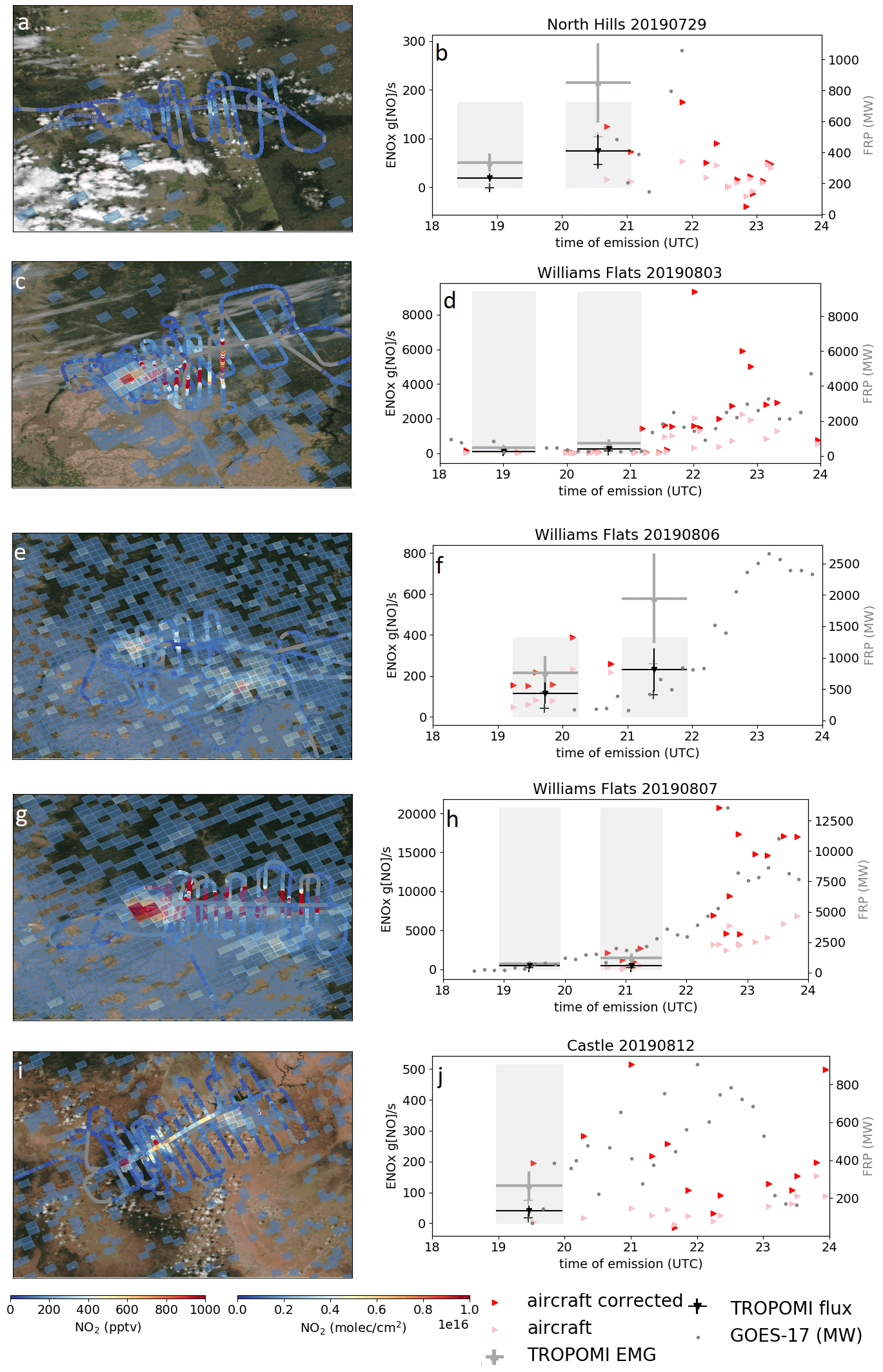
Figure 9 Comparison between aircraft and TROPOMI NO_x emission rate estimates. Aircraft data were collected as part of the FIREX-AQ campaign on the DC-8; for five flights aircraft and TROPOMI measurements are coincident. The TROPOMI VCD_EC ($>\mathrm{1}\times {\mathrm{10}}^{\mathrm{15}}$ molec/cm²), together with the aircraft NO₂ (in pptv) and VIIRS overlays (obtained from NASA Worldview; https://worldview.earthdata.nasa.gov/, last access: 10 December 2021​​​​​​​), is shown on the left. The aircraft-derived emissions are shown as pink and red triangles. The red triangles are the aircraft-derived emissions corrected assuming a lifetime of 2 h. The TROPOMI-derived emissions are estimated with the EMG (grey) and flux (black) method utilizing the VCD_EC (triangles) and as a comparison VCD_KNMI (crosses). The grey shaded areas indicate the times when the aircraft- and satellite-derived emissions were coincident. The aircraft-derived emissions have an uncertainty of 20 %–60 % (not shown here) that can be seen in the spread. The GOES FRP in MW (right axis) is shown as small grey dots and indicates the change in the fire activity during the day.

Table 2 Summary of the satellite (using VCD_EC for the estimate) and aircraft-derived NO_x emission estimates (in t[NO]/h). The uncertainties for the satellite-derived emissions are based on Table 1, and the aircraft-derived uncertainties are approximately 40 %.

5.3 DOAS comparison

As a third comparison, we included the DOAS observations taken as part of the BB-FLUX campaign, here referred to as CU-DOAS. A total of three flights and three TROPOMI overpasses were found to be near-synchronous with good coverage of TROPOMI and aircraft-measured NO₂. The flights measured the Rabbit Foot Fire (Idaho, US) on 12 and 15 August 2018 and the Watson Creek Fire (Oregon, US) on 25 August 2018. The flights were roughly 30 min to 1 h different from the TROPOMI overpass times. To take this into account, a plume age is estimated using the FLEXPART-WRF model, following the approach of Theys et al. (2020). The measurements are considered to be inside the plume if the NO₂ columns are greater than 3×10¹⁵ molec/cm²; this threshold has been chosen to avoid measurements too close to the plume edge. Figure 10 shows the TROPOMI and aircraft comparisons: maps of both measurements are shown on the left panels with the VIIRS overlay, and the plume age of these measurements is shown on the right panels for all three flights for the TROPOMI VCD_EC (original VCD_KNMI can be found in the Appendix). There is good agreement between the aircraft and TROPOMI VCD_EC NO₂ columns; the mean differences (CU-DOAS − TROPOMI) are $-\mathrm{0.27}\pm \mathrm{3.71}\times {\mathrm{10}}^{\mathrm{15}}$ molec/cm² (−4 %) ($-\mathrm{1.66}\pm \mathrm{4.95}\times {\mathrm{10}}^{\mathrm{15}}$ molec/cm² for VCD_KNMI) and $\mathrm{1.3}\pm \mathrm{3.0}\times {\mathrm{10}}^{\mathrm{15}}$ molec/cm² (20 %) ($\mathrm{2.56}\pm \mathrm{2.86}\times {\mathrm{10}}^{\mathrm{15}}$ molec/cm² for VCD_KNMI) for the Rabbit Foot Fire on 12 and 15 August, respectively. The differences are calculated by estimating average aircraft columns that were observed within ±10 min of the TROPOMI plume age, as shown in Fig. 10 (right panels). The best coverage of the Watson Creek Fire is not available for a good comparison, as the aircraft measurements span a range between 3×10¹⁵ and 3×10¹⁶ molec/cm², and the time difference between the aircraft and the satellite is greater than 1 h. From Fig. 10f it appears that the aircraft and satellite VCDs are in good agreement, except for the peak that was seen from the aircraft.

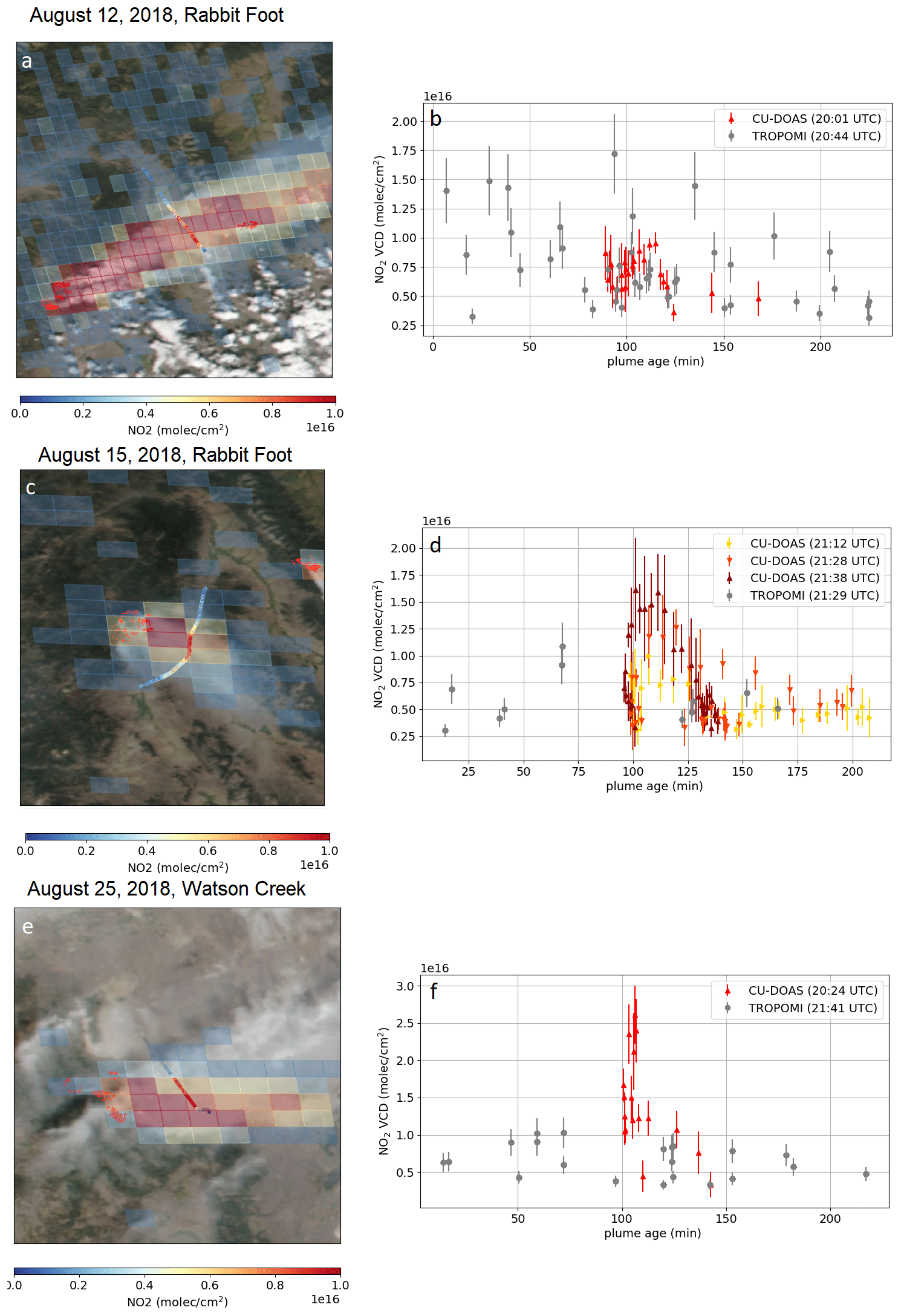
Figure 10 Comparison between the BB-FLUX aircraft measurements (CU-DOAS; 10 s averages are shown together with the corresponding standard deviation) and TROPOMI NO₂ VCDs (VCD_EC). The maps with the satellite pixels and aircraft transects are shown in the panels on the left (a, c, e). The overlay is a VIIRS true-colour image with the MODIS fire hotspots, shown as red dots (obtained from NASA Worldview; https://worldview.earthdata.nasa.gov/, last access: 10 December 2021​​​​​​​). The plume age for pixels with VCD $>\mathrm{1}\times {\mathrm{10}}^{\mathrm{15}}$ molec/cm² is shown in the panels on the right (b, d, f) for the TROPOMI VCD_EC (grey) and the CU-DOAS VCDs (yellow, orange and red). The time of the observations is displayed in the legend.

From the CU-DOAS aircraft measurements NO₂ emission fluxes were estimated by integrating the columns for the entire plume transect and multiplying these by the wind speeds. Wind speed and direction were derived from in-plume profiles made in between plume underpasses. The results are summarized in Table C2, where the emission estimates for the EMG and the flux method are included using the VCD_EC columns (the same table but using VCD_KNMI is included in the Appendix). The emissions are lower when applying the flux method to the satellite observations, similar to the comparison with the FIREX-AQ emission estimates. In the sensitivity tests, however, the flux-method-derived emissions are biased high. This could be due to the different lifetime of NO_x in the model analysis compared to the real measurements; for very short lifetimes, the flux-method-derived emissions can change significantly. The agreement between the satellite- and CU-DOAS-derived emissions is very good when using the EMG method, but the emissions are underestimated with the flux method for the Rabbit Foot Fire on 15 August and the Watson Creek Fire. The Rabbit Foot Fire measured on 12 August 2018 is the only fire where the TROPOMI emissions are high-biased compared to the aircraft emissions. However, this plume was measured further downwind (roughly 40 km) than the other fires, and some of the NO₂ might have decayed. The other two plumes were measured much closer to the fire (roughly 20 km). Some differences are also expected due to the different time of emissions; the CU-DOAS plume observed a plume age of roughly 2 h, and as discussed in the previous section, the time of emission for the TROPOMI estimates is 30±30 min prior to the overpass.

Table 3 Summary of the satellite (using VCD_EC for the estimate) and CU-DOAS NO₂ emission estimates.

6 Conclusions

Based on our analysis, we conclude that estimating biomass burning NO_x emissions from single TROPOMI overpasses is possible with both a flux method and the EMG method, assuming that certain (low cloud cover, no pyrocumulus development, and consistent winds) conditions are met. Estimating biomass burning emissions from single overpasses is desirable as biomass burning emissions can change very quickly. Using synthetic data from an air quality model with prescribed emissions, we showed that the input emissions can be reproduced with either method. More consistent and better correlations are achieved with the EMG method, which also showed smaller uncertainties (38 %) compared to the flux method (53 %). The primary contributor to the uncertainties is the NO_x lifetime, while winds contribute secondarily. It is important for wind speed and wind direction to be accurate; however, the EMG estimate is stable when the winds are a little inaccurate or uncertain. The main contributors to the overall uncertainty of the flux method are the uncertainties of the method itself, the lifetime (only if the lifetime is short), and the wind speed. Using model output and aircraft observations, the NO₂-to-NO_x scaling that needs to be applied to (early afternoon) satellite-derived NO₂ emissions is stable for forest fires. Based on model results and aircraft measurements, TROPOMI-derived emissions of NO₂ should be scaled by a factor of 1.3 to 1.5 to obtain total emissions of NO_x (which, at the point of emission, will largely be in the form of NO). For the NO_x lifetime we derived 2±1 h using the EMG for various fires. This is in good agreement with the results from the WE-CAN campaign that suggested a NO_x decay time of 90 min in biomass burning plumes (Juncosa Calahorrano et al., 2021).

We further investigated the effects of an explicit aerosol correction on the AMF and consequently on the derived emissions. A comparison to aircraft-based integrated profiles and aircraft-derived emissions showed improvement by using the aerosol-corrected AMFs over the original AMFs that rely on an implicit aerosol correction that assumes aerosols as clouds. Applying an explicit aerosol correction to the TROPOMI AMFs improves the TROPOMI NO₂ VCDs. The new VCD_EC showed better agreement with aircraft-observed VCDs over the standard product (VCD_KNMI).

When looking at fire emissions it is important to keep the diurnal variability in mind. TROPOMI measures at roughly 13:30 local time; at this time the fire activity is typically increasing (unless there is rain or the fire is extinguished), and emissions before the overpass were likely smaller than at the time of the overpass. This will impact the lifetime estimate using satellite observations and will likely not return the correct lifetime. The diurnal variability also needs to be kept in mind when comparing to aircraft-derived emissions; therefore, it is important to compare emission estimates for coincident times of emissions to limit the impact by the diurnal variability on the comparison. For the comparison between the TROPOMI-derived and aircraft-derived emissions during FIREX-AQ and the BB-Flux campaign, we found agreement between the satellite-derived emissions using the flux method or EMG method and the aircraft-derived emissions. The flux method always resulted in lower emissions compared to the EMG method and usually underestimated the aircraft-derived emissions during FIREX-AQ and the BB-FLUX campaign. There is better agreement when the EMG method is applied using the VCD_EC, and the aircraft- and satellite-derived emissions are typically within the estimated uncertainties. We would recommend using the EMG method for estimating NO_x fire emissions from TROPOMI single overpasses.

Overall, we conclude that fire emissions of NO_x can be determined from the TROPOMI dataset and showing good agreement with aircraft-derived emissions. While this study focuses on forest fire emissions in North America, based on the availability of aircraft-borne measurements, fire emissions from TROPOMI can be derived globally and for different types of vegetation. This can be helpful to evaluate the input emissions of air quality models and to determine an overall annual emission budget of wildfires. However, TROPOMI typically has a single daily overpass in the afternoon that can only provide limited information on the diurnal variability of the emissions. Future geostationary satellites, like the Tropospheric Emissions: Monitoring of Pollution (TEMPO) mission, will be able to give further insight into the diurnal variability, and the same methods can be applied to these observations. The combination of emission coefficients (amount of NO_x per MW) together with the geostationary GOES FRPs might also be useful to address the diurnal variability of fires and the total daily, monthly, or annual emissions. As shown for the FIREX-AQ fires (Fig. 9), the GOES FRP is a good indicator of NO_x fire emissions and tracks the emissions well. In a future study, we will look further into TROPOMI emissions and GOES-FRP to obtain more information on diurnal patterns and to obtain a total NO_x budget from biomass burning in North America.

Appendix A: Exponentially modified Gaussian

The EMG method describes a Gaussian-shaped plume in the crosswind (x) and along-wind (y) direction. The fit is performed in a Python script using the SciPy package using the Levenberg–Marquardt algorithm, which minimizes the difference between the fitted VCDs and the satellite-observed VCDs, where we use Eq. (A1) and find the best solution (for a, B, and occasionally λ and σ – depending on whether these are held constant or are fitted, as described in the text) with scipy.optimize.curve_fit (method = “lm”). The following equations are used to describe the Gaussian plume; the wind speed s is needed for this, and the decay rate λ (inverse of the lifetime) can either be fitted or can be a fixed parameter; similarly, the plume spread σ can be fitted or be a fixed parameter.

$$\begin{array}{}\text{(A1)}& {\mathrm{VCD}}_{{\mathrm{NO}}_{\mathrm{2}}}(x,y,s)=a\cdot f(x,y)\cdot g(y,s)+B\end{array}$$

From the enhancement factor a the emissions can be determined by $E=a\cdot \mathit{\lambda }$. The functions f(x,y) and g(y,s) describe the plume shape:

$$\begin{array}{}\text{(A2)}& {\displaystyle }f(x,y)={\displaystyle \frac{\mathrm{1}}{{\mathit{\sigma }}_{\mathrm{1}}\sqrt{\mathrm{2}\mathit{\pi }}}}\cdot \exp \left({\displaystyle \frac{-x^{\mathrm{2}}}{\mathrm{2}{\mathit{\sigma }}_{\mathrm{1}}^{\mathrm{2}}}}\right),\text{(A3)}& {\displaystyle }g(y,s)={\displaystyle \frac{{\mathit{\lambda }}_{\mathrm{1}}}{\mathrm{2}}}\cdot \exp \left({\displaystyle \frac{{\mathit{\lambda }}_{\mathrm{1}}({\mathit{\lambda }}_{\mathrm{1}}\cdot {\mathit{\sigma }}^{\mathrm{2}}+\mathrm{2}y)}{\mathrm{2}}}\right)\cdot \mathrm{erfc}\left({\displaystyle \frac{{\mathit{\lambda }}_{\mathrm{1}}{\mathit{\sigma }}^{\mathrm{2}}+y}{\sqrt{\mathrm{2}\mathit{\sigma }}}}\right).\end{array}$$

The crosswind and downwind coordinates are described by x and y in kilometres (km), the wind speed s is in kilometres per hour (km/h), and the plume spread (describing the width of the Gaussian plume) is σ in kilometres (km). λ is the decay rate and the inverse of the lifetime $\mathit{\tau }(=\mathrm{1}/\mathit{\lambda })$ in h⁻¹, and λ₁ is short for $\mathit{\lambda }/s$ (inverse of the lifetime over the wind speed). B is the background column, and a is the enhancement factor in molecules per square centimetre (molec/cm²). “erfc” is the complementary error function and is included in SciPy (scipy.special.erfc). σ₁ is described differently upwind and downwind of the fire hotspot:

$$\begin{array}{}\text{(A4)}& {\mathit{\sigma }}_{\mathrm{1}}=\left\{\begin{array}{ll}\sqrt{{\mathit{\sigma }}^{\mathrm{2}}-\mathrm{1.5}y}& ,y<\mathrm{0}\\ \sqrt{\mathit{\sigma }}& ,y>\mathrm{0}.\end{array}\right.\end{array}$$

Further details about the EMG can also be found in other publications, e.g. Fioletov et al. (2015) and Dammers et al. (2019).

Appendix B: Sensitivity to lifetime and plume spread

Using a different lifetime and plume spread does have an impact on the bias to the true emissions; however, the correlation is not affected by this. Note that changes in lifetime and plume spread can compensate for each other. For the previous cases, discussed in Sect. 4.2, we use a plume spread and lifetime of 6 km and 1 h (note that this does not represent the true chemical lifetime). Figure B1 shows the variation of the slope of best fit of the fitted emissions to the true emissions: a lower lifetime will increase the emissions, and a lower plume spread will decrease the emissions. Thus, the emissions are almost identical when using σ=9 km, τ=2 h, and σ=7 km, τ=1.5 h. Based on this analysis, the uncertainty is about 25 % within the associated spread of lifetimes and plume spreads. This is a major contributor of uncertainty, and thus it is important to find a realistic lifetime to reduce the overall uncertainties of the emissions estimate, which is not always easy.

Figure B1 The impact of changing the lifetime and plume spread parameter on the slope of best fit (under a (i) scenario) using the EMG method to obtain the fitted emissions.

Appendix C: EMG without restrictions

Based on our analysis, we recommend using the EMG with restricted lifetime and plume spread. The results when the EMG is used to estimate the emissions, lifetime, and plume spread simultaneously are presented below.

Table C1 Summary of the satellite (using VCD_EC for the estimate) and aircraft-derived NO_x emission estimates (in t[NO]/h). For the TROPOMI estimates we used the EMG to derive emissions, lifetime, and plume spread. Note that the first guess parameter for lifetime was 4 h; sometimes when a solution cannot easily be found the algorithm defaults to the first guess parameter.

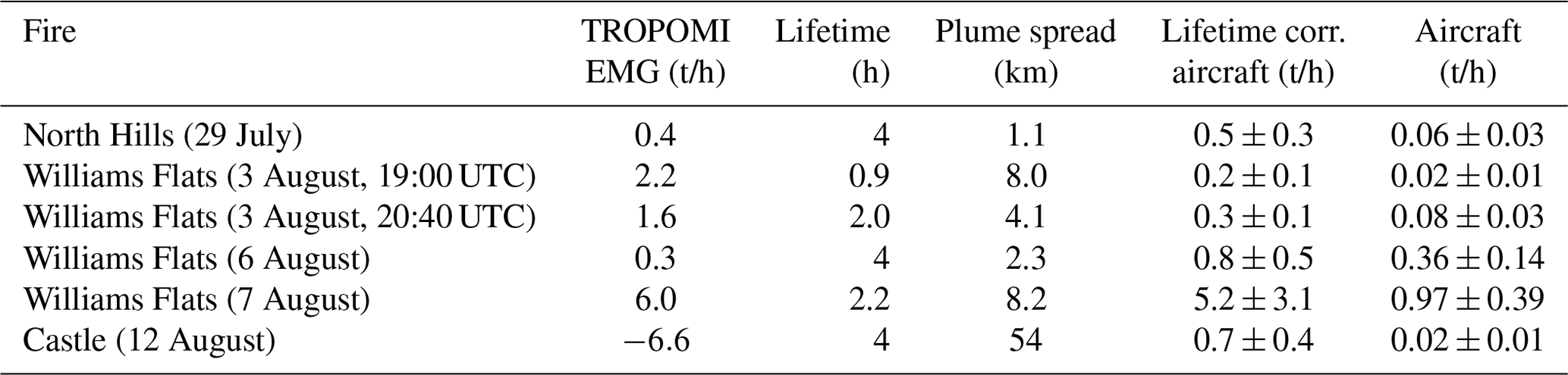
Table C2 Summary of the satellite (using VCD_EC for the estimate) and CU-DOAS NO₂ emission estimates. For the TROPOMI estimates we used the EMG to derive emissions, lifetime, and plume spread. Note that the first guess parameter for lifetime was 4 h; sometimes when a solution cannot easily be found the algorithm defaults to the first guess parameter.

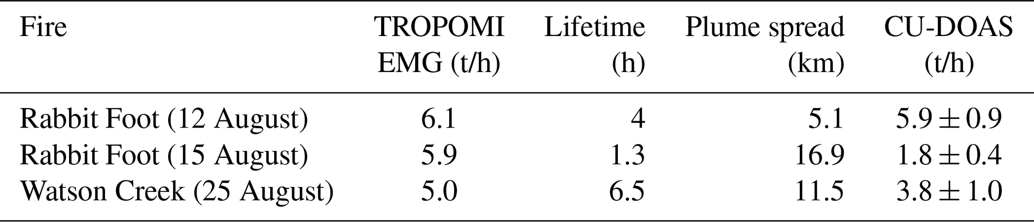
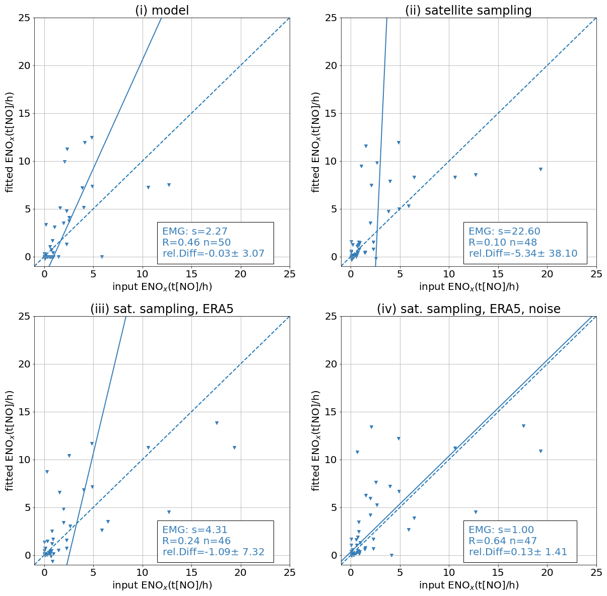
Figure C1 The results of the sensitivity test with synthetic data for test (i)–(iv) are illustrated (see text for detailed description of the scenarios). The fitted emissions applying the EMG method that simultaneously fits the lifetime and the plume spread (blue downward triangles) versus the model input emissions are plotted together with the statistics (slope of best fit using the geometric mean, s; correlation coefficient, R; the number of points, n; and the mean and standard deviation of the relative difference, rel. Diff: input − fitted).

Appendix D: AMF with changing AOD

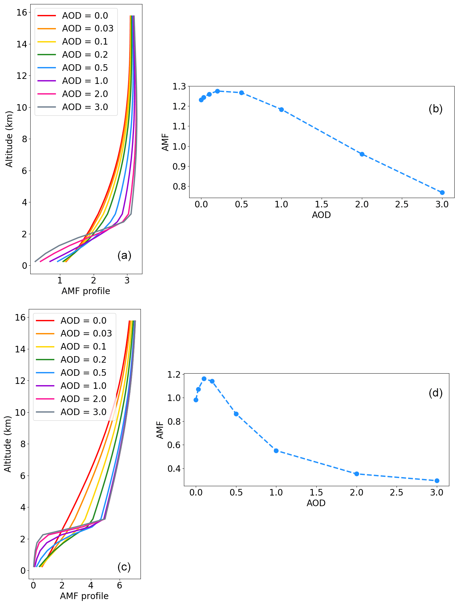
Figure D1 This figure illustrates the changes in AMF with changing AOD. The altitude-dependent AMF profile is shown in panel (a) and (c) for an aerosol layer height of 3 km with a changing AOD. Panel (b) and (d) show the total integrated AMF versus the AOD using a typical temperature profile. The difference between the top panel and bottom panel is the viewing geometry. (a, b) VZA = 50^∘, SZA = 50^∘, and DAZ = 60^∘ and (c, d) VZA = 70^∘, SZA = 78^∘, and DAZ = 150^∘, where VZA is the viewing zenith angle, SZA is the solar zenith angle, and DAZ is the difference between the solar and viewing azimuth angle. The surface pressure is 1000 hPa and the albedo is 0.09 in both examples.

Appendix E: Aircraft comparison using VCD_KNMI

Table E1 Summary of the satellite (using VCD_KNMI for the estimate) and CU-DOAS NO₂ emission estimates.

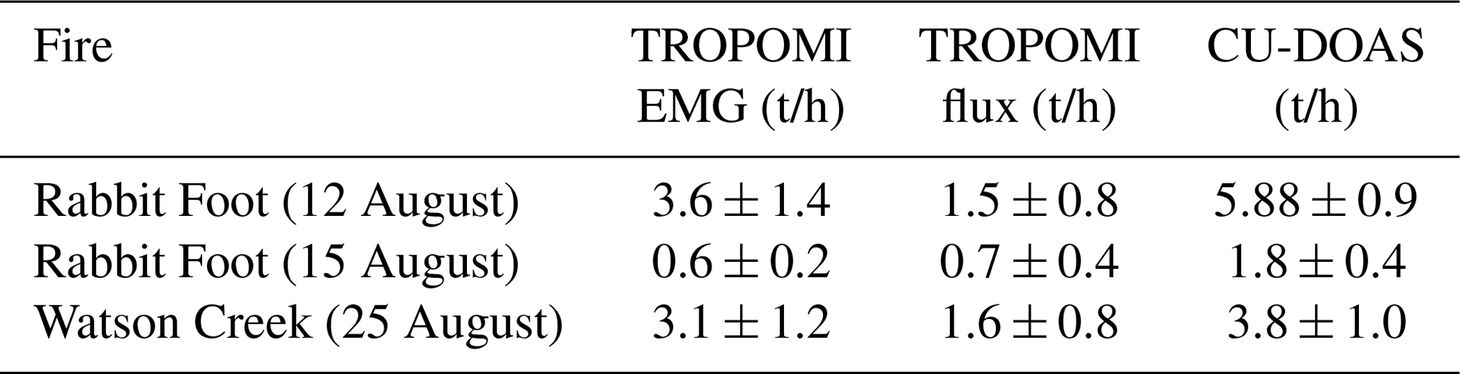
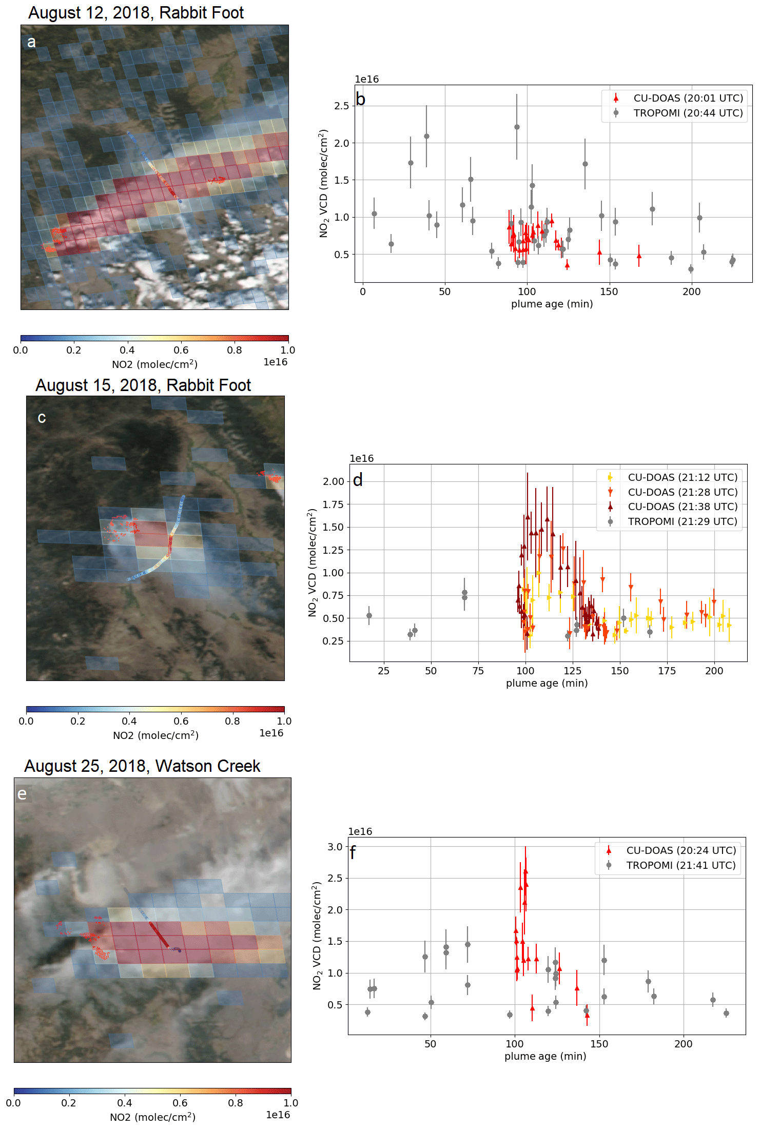
Figure E1 Same as Fig. 10 but for the TROPOMI VCD_KNMI instead. The mean difference is $-\mathrm{1.75}\pm \mathrm{4.51}\times {\mathrm{10}}^{\mathrm{15}}$ molec/cm² (−26 %) and $\mathrm{2.21}\pm \mathrm{1.56}\times {\mathrm{10}}^{\mathrm{15}}$ molec/cm² (32 %) for the Rabbit Foot Fire on 12 and 15 August, respectively.