the Creative Commons Attribution 4.0 License.
the Creative Commons Attribution 4.0 License.
 | 23 Dec 2021
Photochemical method for removing methane interference for improved gas analysis
Merve Polat
Jesper Baldtzer Liisberg
Morten Krogsbøll
Thomas Blunier
The development of laser spectroscopy has made it possible to measure minute changes in the concentrations of trace gases and their isotopic analogs. These single or even multiply substituted species occur at ratios from percent to below parts per million and contain important information concerning trace gas sources and transformations. Due to their low abundance, minimizing spectral interference from other gases in a mixture is essential. Options including traps and membranes are available to remove many specific impurities. Methods for removing CH4, however, are extremely limited as methane has low reactivity and adsorbs poorly to most materials. Here we demonstrate a novel method for CH4 removal via chlorine-initiated oxidation. Our motivation in developing the technique was to overcome methane interference in measurements of N2O isotopic analogs when using a cavity ring-down spectrometer. We describe the design and validation of a proof-of-concept device and a kinetic model to predict the dependence of the methane removal efficiency on the methane concentration [CH4], chlorine photolysis rate , chlorine concentration [Cl2] and residence time tR. The model was validated by comparison to experimental data and then used to predict the possible formation of troublesome side products and by-products including CCl4 and HCl. The removal of methane could be maintained with a peak removal efficiency >98 % for ambient levels of methane at a flow rate of 7.5 mL min−1 with [Cl2] at 50 ppm. These tests show that our method is a viable option for continuous methane scrubbing. Additional measures may be needed to avoid complications due to the introduction of Cl2 and formation of HCl. Note that the method will also oxidize most other common volatile organic compounds. The system was tested in combination with a cavity ring-down methane spectrometer, and the developed method was shown to be successful at removing methane interference.
- Article
(7638 KB) - Full-text XML
- BibTeX
- EndNote


Infrared absorption is a fast, convenient and non-destructive approach for measuring gas composition that is used in a wide range of applications. High-resolution instruments based on specific rovibrational transitions are becoming available to characterize the abundance of rare isotopocules within gases. Laser spectroscopy has entered territory that has been the exclusive domain of mass spectrometry. While recent advances in the field can give the impression that new laser-based instruments can be used in a “plug and play” manner, there are still limitations to the accuracy and reproducibility of the measurements.
In a recent study investigating the performance of currently available laser spectroscopic N2O isotope analyzers (Harris et al., 2020), a number of interferences from other trace gases were identified, arising from spectral overlap of N2O and the rovibrational spectra of the other gases. The consequence was an offset in the measured isotopocule abundance value arising exclusively from ambient levels of methane for a Picarro G5131-i cavity ring-down-based instrument that determines δ15N, δ15Nα, δ15Nβ and δ18O for N2O. These instruments are often used to measure isotopic signatures of N2O emitted from soils, (Ibraim et al., 2019; Wolf et al., 2015; Yu et al., 2020), which can help to differentiate distinct microbial and abiotic production pathways.
N2O formation in soils is commonly accompanied by production and/or uptake of other trace gases such as CH4, CO2 and water vapor (Erler et al., 2019; Ibraim et al., 2019). These variations complicate measurements. An example of the relevant variation of CO2 and CH4 can be found in the work of M. Zimnoch and Rozanski (2010) in which the background level of CH4 and CO2 at 1.8 and 380 ppm can change suddenly to levels above 3.6 and 560 ppm. For the instrument described in Harris et al. (2020), these variations will result in an observed offset in the measured δ15Nα of 4.0 ‰ and δ18O of 1.1 ‰ (Harris et al., 2020). The change in CH4 results in an apparent increase of 4.6 ‰ and 2.2 ‰ for δ15Nα and δ18O, respectively, while the change in CO2 results in a decrease of 0.6 ‰ and 1.1 ‰ for δ15Nα and δ18O, respectively. As the effect of variation in these two trace gases leads to opposing offsets in the measured isotopologues, it greatly decreases both the accuracy and precision of the G5131-i. It is therefore essential for accurate measurements to account for these interferences.
One solution is multi-line analysis or careful measurement of the interfering gas(es) with a second instrument. These options are not desirable for all applications as they either require a redesign of the instrument or investment in additional equipment, and these corrections can introduce additional uncertainty. A more direct and practical method would be to remove the interfering species from the sample. For discrete sampling the best method would be to separate the N2O from the sample matrix and release it into a well-defined matrix for interference-free measurements.
For online measurements, well-established methods including chemical traps and membranes are readily available for the removal of CO2, CO and humidity. However, to the best of our knowledge, no method for continuous removal of methane is available with the exception of catalyzed combustion (Cullis and Willatt, 1983), which requires high temperatures and the addition of oxygen, thereby altering the gas matrix. It was desired to develop a method for removing CH4 and potentially other volatile organic compounds (VOCs) in a manner that would only introduce minimal changes to the matrix composition.
Inspiration for the method investigated in this work was taken from the oxidation pathways taking place in the atmosphere (Pugliese, 2018). The majority of methane is oxidized through an initial reaction with OH radicals (Rigby et al., 2017) that results in the formation of H2O and CH3 radicals. However, the chlorine radical is a potentially important agent for initiating chain reactions: generally, the reaction rates of Cl with VOCs exceed the analogous ones with OH by at least 1 order of magnitude. The rate constant for methane reaction with Cl radicals is cm3 s−1 (Bryukov et al., 2002) and with hydroxyl radicals is cm3 s−1 (Bonard et al., 2002). The reason for the limited role of chlorine in the global atmosphere is that its concentration on average is 3 or 4 orders of magnitude lower than OH, although it can have an impact in the stratosphere and in marine and polar environments. The mechanism for Cl-initiated methane oxidation technology proposed in this study is outlined in Reactions (R1)–(R6).
We demonstrate a novel method for CH4 removal through chlorine-initiated oxidation. Using four experimental setups, we show that methane removal is highly dependent on the flow, chlorine mixing ratio and light source. We developed a simple kinetic model to predict the removal efficiency as a function of the four key parameters in the system: [CH4], , [Cl2] and residence time tR. The model includes essential reactions and additional estimated radical wall reactions. Two approaches for estimating the photodissociation rate of Cl2 are presented. The goal is to determine the effect of these variables and achieve the desired methane removal efficiencies by optimizing the parameters. The goal is to achieve removals above 99 % for methane at low to ambient concentrations. With the method developed and refined, a final set of experiments is conducted using a Picarro CRDS model G5131-i capable of measuring N2O mixing ratio and its isotopic abundance. The measured values of δ15Nα and δ18O, subject to methane interference, are compared to data corrected for methane levels, as these corrected isotopologue levels remained stable across the experiment.
2.1 Experimental approach
2.1.1 Methane experiments
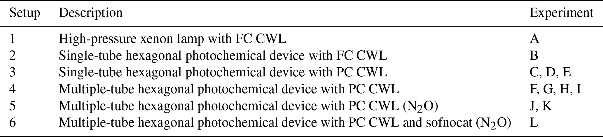
Four different variations of the setup seen in Fig. 1 are used during our experiments and are summarized in Table 1 together with the experiments they were used for.
Table 1Table summarizing experiments and setups. See Fig. B1 for an overview. FC: flow-controlled. CWL: chlorine waste line. PC: pressure-controlled.
Figure 1General setup. ACT: activated carbon trap. MFM: mass flowmeter. MFC: MKS mass flow controller GE50A. MFC: manual flow controller. Table 2: gas flask. Four variations of the general setup are performed. The setup variations and the experiments performed with the setups are shown in Table 1. Setup 1 uses a xenon lamp as the photochemical device. Setups 2–4 use the same photochemical device, which consists of 420 LEDs. The chamber tube used in setups 1–3 is one quartz tube (20 cm length × 12.7 mm o.d.), while setup 4 uses seven smaller quartz tubes: five with the size 8.33 mm (o.d.), 6.33 mm (i.d.) and 20 cm (L), as well as two with the size 8.33 mm (o.d.), 6.33 mm (i.d.) and 25 cm (L). The setups also differ in the chlorine waste line. Setups 1–2 use a flow-controlled chlorine waste line, while setup 3.4 uses a pressure-controlled chlorine waste line.
The system (Fig. 1) has a manifold combining flows from two channels: the sample channel and the chlorine gas channel. [Cl2] is supplied from an external tank labeled flask I (see Table 2 for gas flask). Atmospheric air in flask II is combined with an enriched source of [CH4] in flask III to generate various levels of [CH4] for the sample channel. A chlorine sensor is placed outside the main flow line to reduce the volume of the setup and allow for increased time resolution. The flow containing methane and chlorine gas is split at a T-piece, where the main flow proceeds through the photochemical device with excess gas going past a Cl2 sensor (chlorine gas detector 0–20 ppm Cl2). Cl2 concentrations above 20 ppm are estimated from the flow rate ratios.
The photochemical device
Setup 1 uses a high-pressure xenon lamp (ILC Technology R100-IB) as the photochemical device. Setups 2–4 use a photochemical chamber consisting of 420 LEDs with peak emission at 365 nm with the circuit board mounted together in a hexagonal cylinder (illustrated in Fig. B2). The 420 LEDs are connected in parallel. At the maximum voltage of 3.8 V each consumes 13.2 mA, resulting in a total power of 21 W.
A single quartz tube with 20 cm length and 12.7 mm outer diameter is used as the chamber tube for setups 1–3. In setup 4, the tR in the chamber is increased by a factor of 2.7 by substituting a single quartz tube with seven smaller quartz tubes in hexagonal shape for optimal packing comprising five tubes with the following dimensions: o.d. 8.33 mm, i.d. 6.33 mm, length 20 cm. An additional two tubes are used with the following dimensions: o.d. 8.00 mm, i.d. 6.00 mm, length 25 cm. The tubes were connected in series via Tygon tubes (Tygon R3603) of length 5 cm. The insides of these tubes were coated with Krytox (DuPont GPL 205 Krytox Performance Grease) to prevent reaction with Cl2.
Post-photolysis scrubbing
After the photochemical device the sample passes through a 35 cm Nafion membrane (TT-030 from Perma Pure LLC). The dried sample then passes through an ascarite trap consisting of a central layer of NaOH between two layers of Mg(ClO4)2 separated by glass wool. These types of traps are normally used for the removal of CO2 and H2O (Harris et al., 2020), but they were found to likewise remove HCl and Cl2. This removal was confirmed by separate experiments, as it was essential that none of the corrosive gases made it to the delicate Picarro instrument. The gas stream then flows into a cavity ring-down spectrometer (CRDS), the Picarro model G1301. A nominal flow of 15 mL min−1 was maintained with the exception of experiments involving variation in tR when this flow was changed accordingly. At the outlet of the Picarro G1301 an activated carbon (bead-shaped activated carbon, KUREHA Corporation) trap labeled ACT is attached, which is mainly used for scrubbing chlorinated organic species, such as CCl4, out of health concern (Ryu and Choi, 2004; Milchert et al., 2000).
2.1.2 N2O experiments
A final set of experiments is conducted using a Picarro CRDS model G5131-i capable of measuring N2O mixing ratio and isotopic abundance. These experiments were performed to validate the effect of the removal of CH4 on the measurement of N2O. These experiments were done in two sets using the setup in Fig. B1b with and without the sofnocat trap. The difference between the two setups was hence the inclusion of a sofnocat trap in Fig. B1b. The sofnocat trap is used to oxidize the CO product (Harris et al., 2020) and was prepared with 1.25 g of sofnocat contained in a stainless-steel tube of length 8 cm kept in place by glass wool.
2.2 Theoretical approach
2.2.1 Kintecus version 6.8
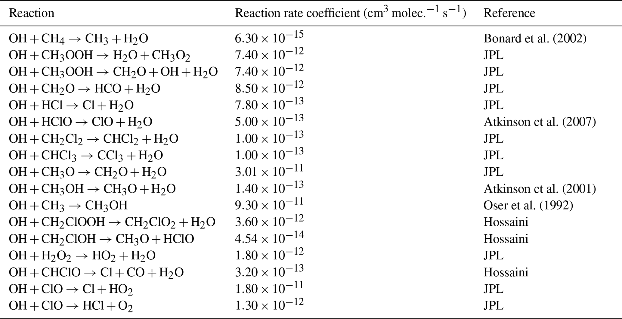
A model is made with the program Kintecus version 6.8 (Ianni, 2012) to investigate the reaction mechanisms in the photochemical device. The model contained the relevant reactions with rates for chlorine radical production and removal, methane oxidation, and formation of chlorinated species. The model was kept as simple as possible while still including the relevant reactions. The reactions used in the model are found in Tables E1–E3. A simplified reaction scheme is shown in Fig. 2. A continuous flow was simulated by setting the initial and external concentrations of gases flowing through the chamber to the same value. This is done for the gases Cl2, CH4, N2 and O2. A copy of the model parameters is available in Appendix C.
Figure 2Reaction scheme for the oxidation of methane to CO2. CH3O2 self-reactions lead to the formation of CH3O.
Radical wall reactions
A set of radical-terminating reactions is incorporated in the model to account for reactions on the walls of the quartz tube.
The wall reactions are assumed to be diffusion-limited. The diffusion length is calculated as the average distance from the wall. The diffusion length and rate were calculated using Eqs. (1) and (2), respectively. The estimate of the diffusion rate is described in detail in Sect. C1. The diffusion constants, diffusion lengths and estimated wall reaction rates are shown in Table C1.
Here, l in the diffusion length and r is the inner radius of the tube.
Here, D is the diffusion constant (see Table C1).
Model results
The outputs from the model are the photodissociation rate, , the abundance of [Cl] and the production of CCl4 as an indicator of the production of unwanted side products.
estimation
The chlorine photolysis rate, , is estimated in two ways, which is described in more detail in Sect. C2. The first approach is to fit to reproduce the observed removal efficiencies from the experimental results. These fits were performed for experiments investigating the effect of power.
A second approach is to estimate by relating it to the electric power going through the circuit, PIN. Based on our observation, a second-order polynomial provided the best fit to describe the effective light output, Peff, as a function of PIN:
where the constants a (W−1) and b (unitless) are experiment-dependent constants that scale the effective light output Peff in watts (W). From the effective power output, the photolysis rate is calculated by Eq. (4).
Jscale (J−1) is the scaling factor and was calculated from the cross section of Cl2, the wavelength distribution of the generated light and the expected photon density. The density of photons depends on the volume and cross section of the tube within the photochemical device. is fit to the data collected for some of the experimental steps for exp. D and I. Exp. D reflects the single-tube system (setups 1–3), while experiment I reflects the optimized multiple-tube system (setup 4). From the fitted a, b and calculated Jscale the photolysis rate could be calculated for the other experiments.
3.1 Experimental results
The findings are based on 12 experiments, named A–L, containing multiple steps of turning on the photolysis under different conditions. These steps will be referred to by their experimental letter and their number; e.g., experiment C step 5 would be exp. C5. An overview of the settings and resulting removal efficiencies for experiments C–I can be seen in Table 3 (see Appendix Tables D1–D3). Table 1 gives an overview of the experiments. As an example of our data, we present the results from experiment H (Fig. 3), during which we achieved our highest level of removal. The experiment was carried out with constant [CH4]initial and [Cl2] at 2.000±0.003 and 50.5 ppm. The different levels of removal seen reflect stepwise changes to the settings for tR and PIN. As seen in Fig. 3 for exp. H1–H4, removal efficiency is improved as the PIN is increased. Starting with H5 a fan was installed to limit temperature increases. PIN was kept at the same level, while the residence time in the chamber was decreased. The three steps (H1–H3) were carried out with constant PIN at 14.8 W with tR ranging from 164–350 s. tR was kept at 350 s for experiments H3–H6. Furthermore, PIN was varied within the range of 14.8–22.8 W. Two issues affected the results. First, the system was not initially stable. We believe this is due to a build-up of moisture on the glass walls coming to equilibrium after the first step, as can be seen from the slope in step H1. Second, there is a small continuous pressure drop from the Cl2 regulator, which leads to a decrease in Cl2 and an increase in CH4. The reason for this was insufficient drying of the regulator prior to use, which left a layer of moisture to react with chlorine, thus initiating corrosion in the regulator. This is also the reason we needed a chlorine waste line, as a high flow through the regulator was needed to reduce the effect of this loss to the regulator. We have accounted for the effect of the pressure drop, but it contributes to the uncertainty of our reported Cl2. We must stress the importance of proper drying prior to the use of Cl2 gas for those intending to emulate our setup.
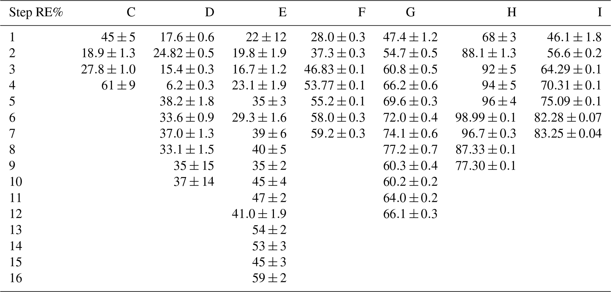
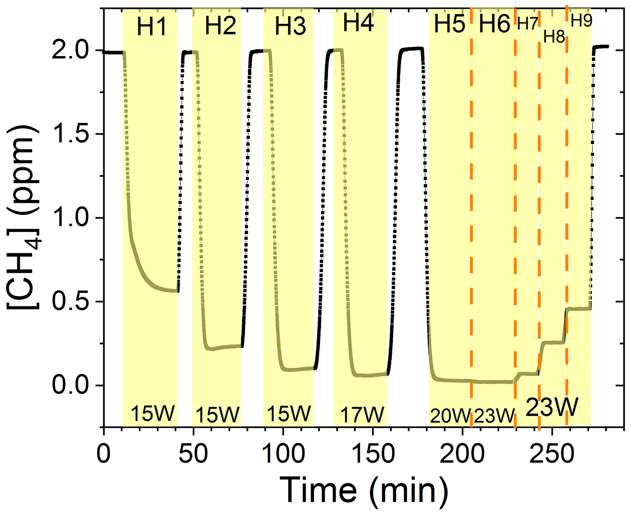
Figure 3Exp. H. The [CH4] is seen as a function of time. The highlighting indicates the illumination times. In addition, the experimental step is indicated at the top and PIN (W) is indicated at the bottom.
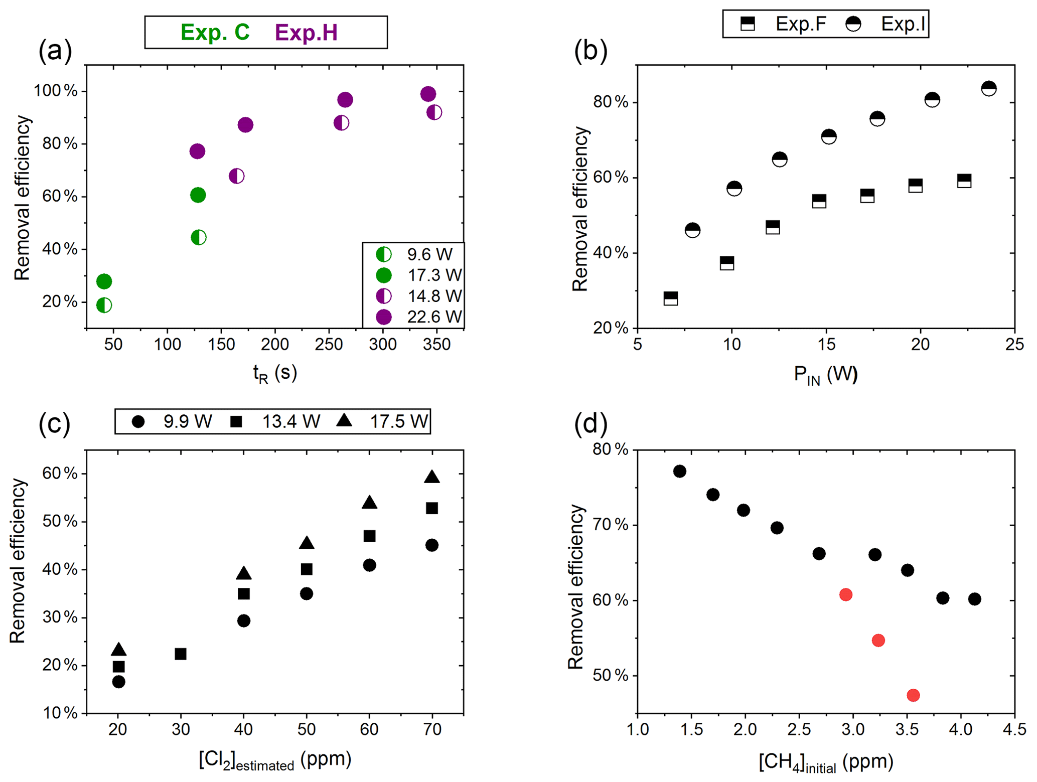
Figure 4(a) RE% of methane plotted against tR (s). The result originates from the two experiments C (green) and H (violet). The experiments have different settings in PIN, [CH4] and [Cl2]. (b) RE% of methane plotted against PIN (W). The results are from the two experiments F (square) and I (triangle), which have different [CH4] settings. (c) The panel presents the methane RE% as a function of the chlorine mixing ratio for exp. E. Step 1, at 30 ppm [Cl2], is an example of start-up deviation; therefore, it is removed. The points represent the three different PIN of the photochemical device. (d) The removal efficiency RE% during exp. G of methane is displayed as a function of the initial methane concentration with the remaining fixed parameters such as [Cl2] mixing ratio, tR and PIN input. The three red points in the figure represent steps suffering from start-up deviation.
Effect of residence time (tR, s)
Increasing the residence time results in increased removal of methane, as shown in Fig. 4a. The tR was investigated in the single- and multiple-tube systems. The same flow rate yields a longer tR for the multiple-tube setup due to the 2.7-fold volume increase. The expected trend of asymptotically approaching 100 % can be seen for exp. H, where the high PIN approaches more quickly. The effective light output and tR are lower for experiments B, C and D compared to H. The resulting removal of methane is accordingly lower. Increasing the tR is an easy way of enhancing the removal but at the expense of a slower response time of the system.
Effect of power input (PIN, w)
The results from experiments with power variations are shown in Fig. 4b. As presented for exp. F the system reaches a maximum removal efficiency such that increasing the power does not yield significantly higher removal efficiencies. The [Cl2] and tR for experiments F and I are found to be 50±4 ppm and 162 mL min−1, respectively. Comparing exp. F to I it is evident that a higher removal efficiency has been reached thanks to the addition of a fan to distribute the heat and prolong the lifetime of the LEDs.
Effect of [Cl2]
Exp. E determined the effect of changing [Cl2]; see Fig. 4c. [Cl2] is set between 20 and 70 ppm. Higher [Cl2] levels result in an increased methane removal rate. The resulting removal efficiency is still below 60 % and the RE% appears to be linear with [Cl2]. Given the result from exp. E the level of [Cl2] was set to 50 ppm for the remaining experiments.
Effect of initial [CH4]
Exp. G, plotted in Fig. 4d, spans [CH4] in the range 1.4–3.8 ppm. Steps G1–G3 are highlighted to indicate the initial instability. The experiment showed high removal of methane at ambient concentrations.
The performance of the experimental setup has been investigated in the aforementioned experiments. The removal efficiencies can be increased by increasing PIN or [Cl2], resulting in an increase in [Cl]. The negative correlation for [CH4] is understandable as RE% is a relative value. As expected, the absolute amount of removed methane scales with the [CH4].
3.1.1 N2O experimental results
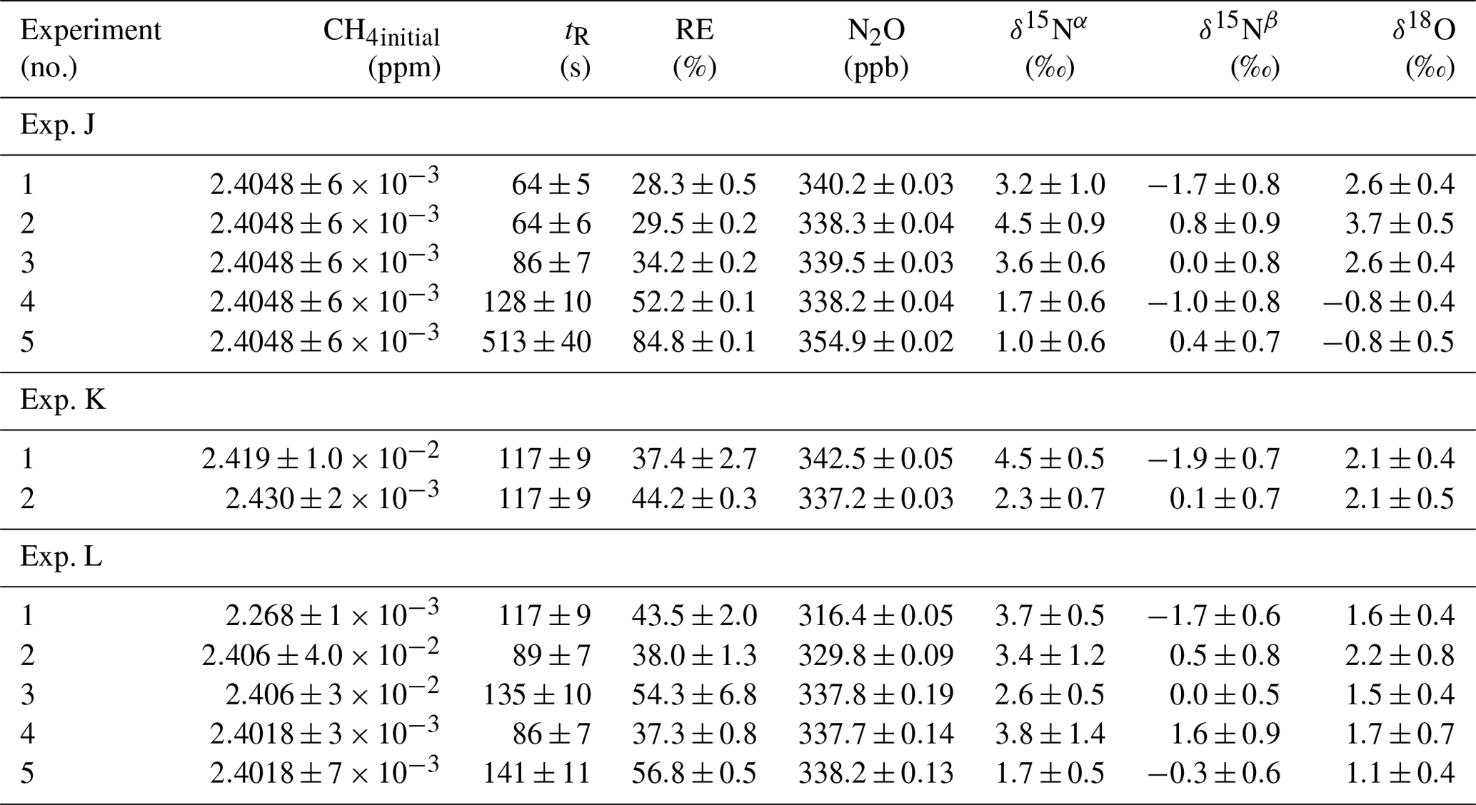
In Fig. 5a and b the effects on the isotopic signal of δ15Nα and δ18O from the removal of methane can be seen. The delta values are self-referenced to the gas without the addition of CH4. The results are from experiment L, wherein a sofnocat trap was installed to remove the CO formed by CH4 oxidation. By applying the trace gas and matrix interference corrections described in Harris et al. (2020) in combination with the measurements of CH4, it was found that the isotopologue levels remained stable through the oxidation (grey line). The offset from this corrected value is plotted in red, showing values higher by several per mill. These levels stabilized during the oxidation in accordance with the drop in methane, thus demonstrating the efficiency of the method. The stability of the corrected isotopic values across the experiment shows that the oxidation does not introduce other components that would interfere with the signal, which are not removed by the traps. Variations of roughly 5 % were observed in [N2O] but are accounted for by variations in the flow of [Cl2], thus changing the dilution, rather than formation of N2O due to the photochemistry. In Table 4 the results from the three experiments J, K and L can be seen. In the N2O experiments it was not possible to apply the same conditions that lead to the highest levels of removal presented in the earlier experiments. The reason for this was that the addition of the G5131-i increased the minimum flow through the photochemical device, thus decreasing the maximum residence time. Additionally, not having a high-concentration N2O source capped the dilution, as the N2O needed to remain in the linear range of the G5131-i. The limit on the dilution therefore also limited the concentration of Cl2 available. With a higher-concentration Cl2 source available and a properly prepared regulator, the setup would have been able to deliver sufficient CH4 removal for more than 24 h, at which point the ascarite trap would need replenishment.
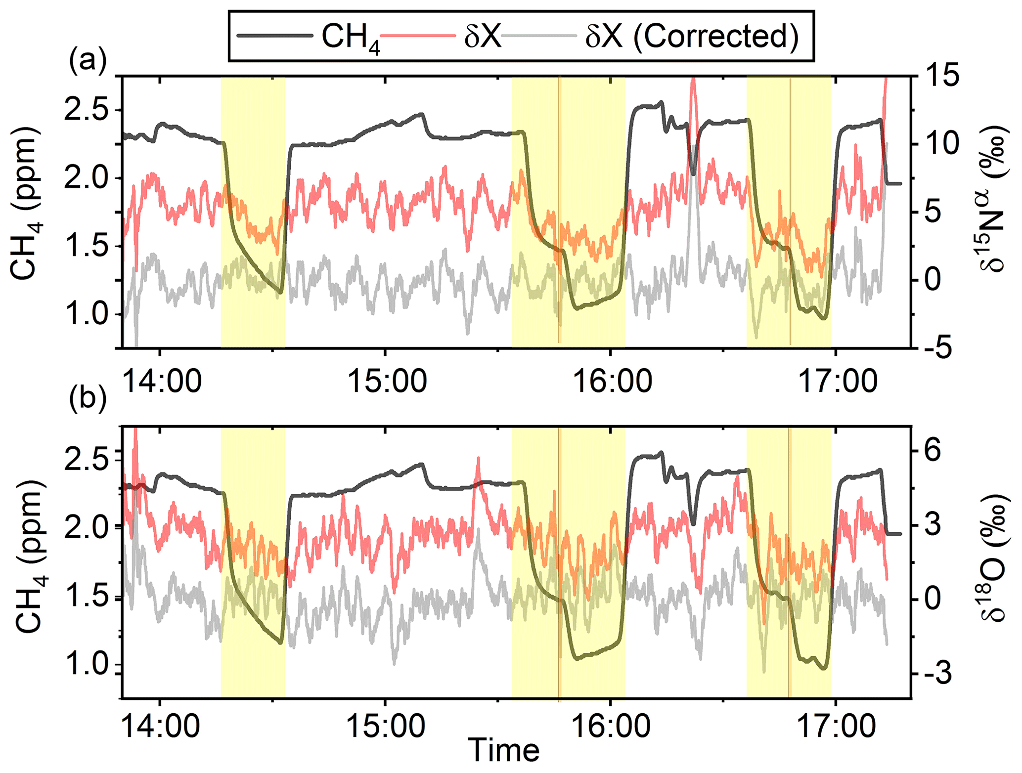
Figure 5(a) Measurements of δ15Nα during exp. L (‰). Red highlights a 100 s average measured value corrected for O2, CO and CO2 effects, while the grey line indicates a 100 s average value corrected for all interference including CH4. The black line shows the CH4 level (ppm). (b) Measurements of δ18O from exp. L (‰). Red highlights a 100 s average measured value corrected for O2, CO and CO2 effects, while the grey line indicates a 100 s average value corrected for all interference including CH4. The black line shows the CH4 level (ppm).
Table 4Experimental data for the N2O experiments using the G5131-i for N2O analysis. Columns: experimental steps, initial [CH4] (ppm), residence time in seconds, removal efficiency in percent (%), [N2O] (ppb), δ15Nα, δ15Nβ and δ18O (‰) refer to the three isotopologue measurements of N2O. Each of the three isotope values have been corrected for the effects of oxygen, CO and N2O variation according to the method described in Harris et al. (2020). The values have not been bound to an absolute scale by the use of calibration gas, so the daily isotope levels unaffected by methane are shown in the day.
3.2 Model results
Parameters a and b in Eq. (3) were determined from the experimental data. For the single-tube system the values were fitted to steps D2 and D6–D9. Here two linear regimes were found and were fitted by two sets of a and b constants. In this way we could describe the effect of the thermal management system used in later experiments.
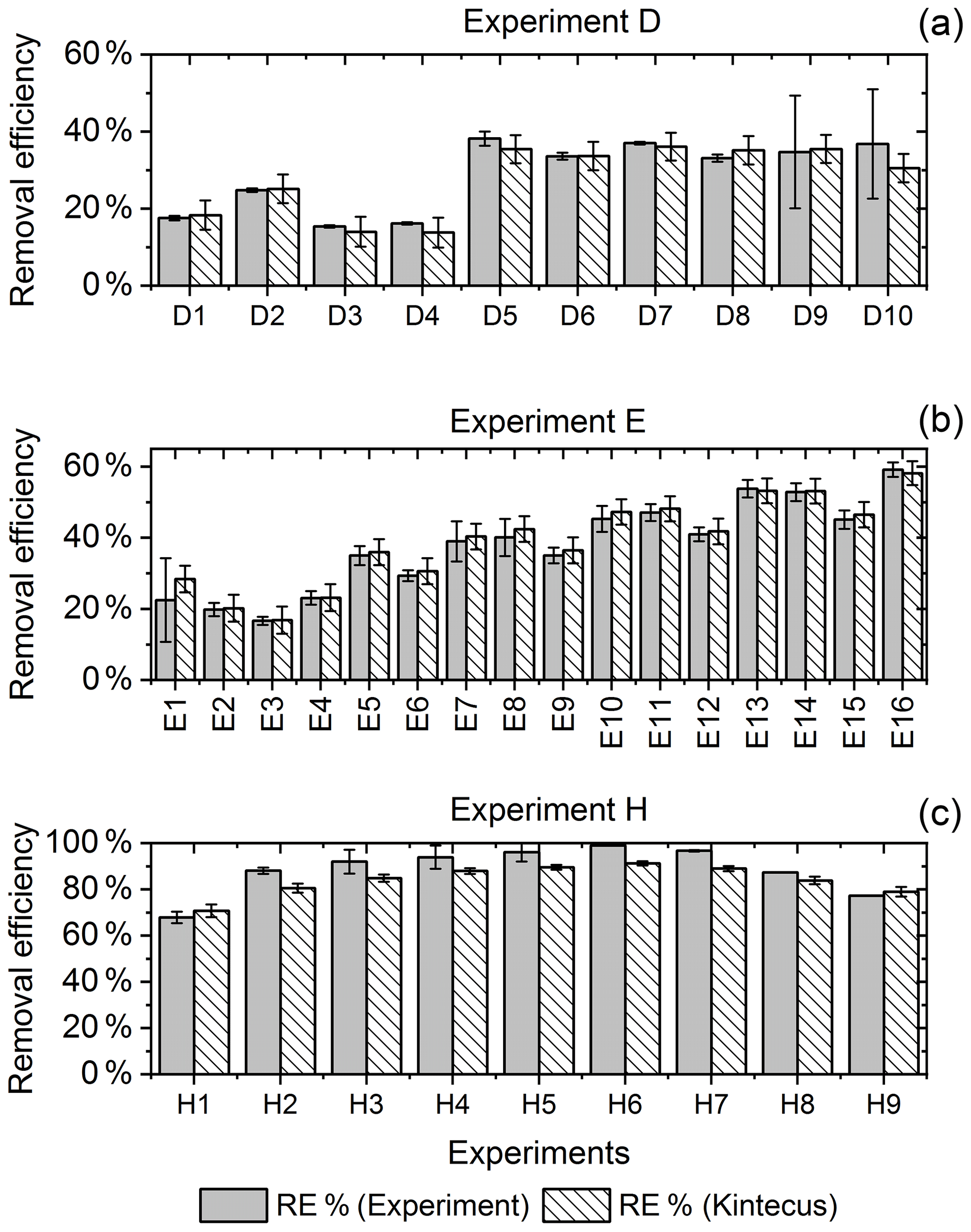
Figure 6RE% for the steps of exp. D, F and H as found experimentally (white stripes) and by the model (grey). (a) Steps D2 and D6–D9 were utilized to generate for the single-tube system. (b) Exp. E and (c) exp. H.
The for the single-tube systems is obtained from Eqs. (C19) and (C20) (Fig. C1c and a). These equations are used to calculate for exp. B, C and D. The comparison between the modeled and experimental efficiency is shown in Fig. 6.
was determined using the same method. Exp. I is used to obtain model (Fig. C1b–C1d and Eq. C21).
In Fig. 6c a comparison of experimental and model results is shown for exp. H, D and E. The model yields good agreement with the experimental results. However, the model slightly underestimates RE% for most of the steps, which is also observed for the other experiments. The initial instability can also be seen for steps D1 and D2 depicted in Fig. 6a. Problems due to overheating at high PIN are eliminated with the improved photochemical device, resulting in a power effectiveness at 15 W of 0.6 % for the single tube to 9 % for the multiple-tube system.
Overall, the simple model does a reasonable job of describing the experimental results, although it underestimates the removal efficiency. One issue is that the model does not do a good job of describing the effect of variations of initial methane concentrations in exp. G, as shown in Fig. E1e.
Additional model runs are used to estimate JCl2 of experiments E and F, which are conducted with a modified device; see Eqs (C22) and (C23)–(C24), respectively. It is clear that adjusting results in a model that more accurately fits the experimental results.
3.2.1 Parameters simulated and compared with experimental results
Exp. I was chosen as the basis for the final simulation: three parameters are fixed and the fourth varies. The methane removal efficiency, chlorine radical abundance and the resulting abundance of [CCl4] are determined. The standard values and the ranges investigated can be seen in Table 5.
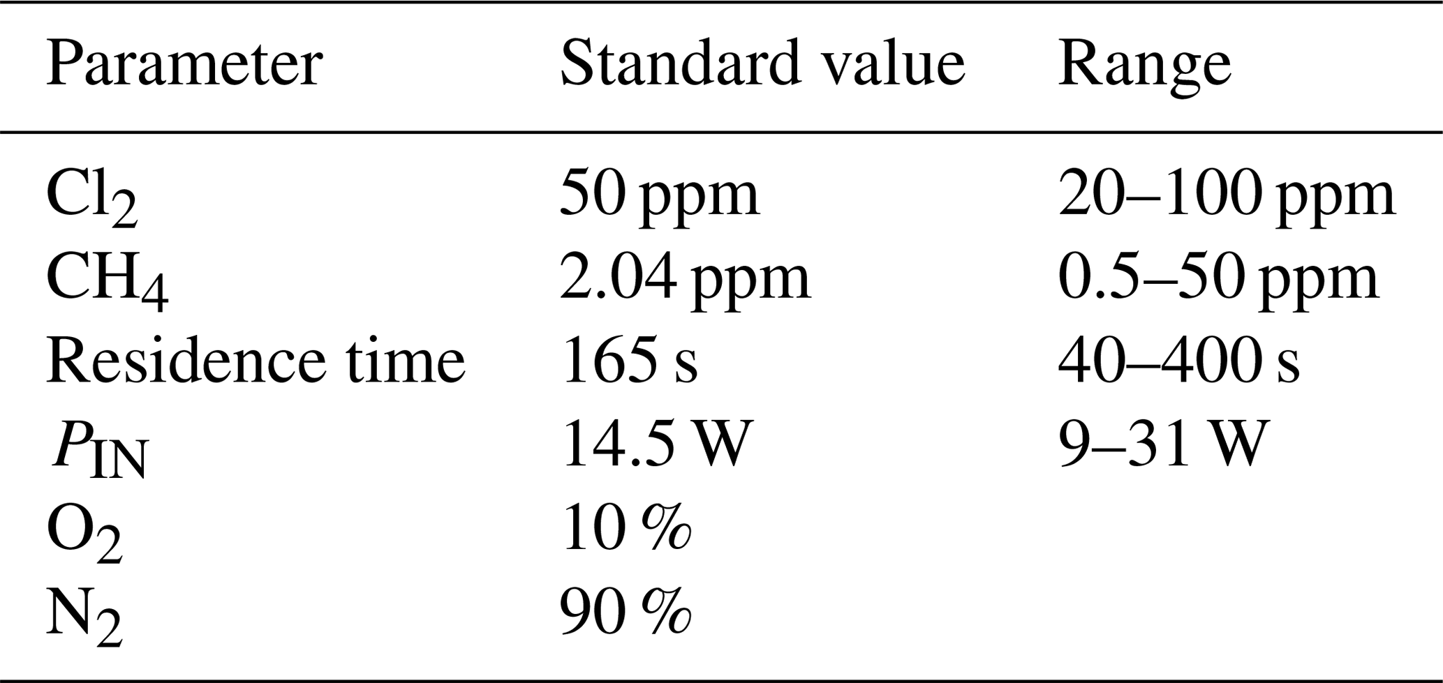
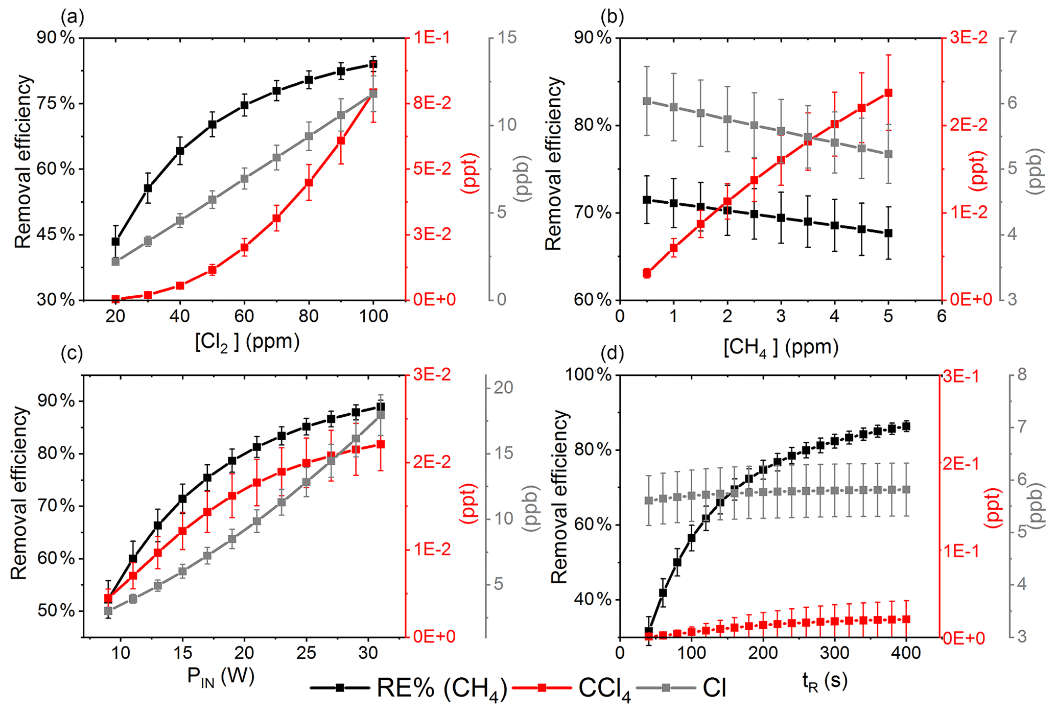
Figure 7The removal efficiency of methane (black), [CCl4] (red) and [Cl] (grey) is shown in panels (a)–(d). The four parameters are varied while the remaining parameters are kept at the standard parameter presented in Table 5. (a) The [Cl2] is varied. (b) The initial [CH4] is varied. (c) The is varied. (d) The tR is varied.
The resulting removal efficiencies as a function of each of the four parameters power input PIN (W), residence time tR (s), [Cl2] (ppm) and [CH4] (ppm) are shown in Fig. 7. The model results are compared with the experimental results for the parameters PIN (W), tR (s) and chlorine mixing ratio (ppm), as shown in Fig. 4b, a and c, respectively. A good match in the observed response can be seen. The model is too insensitive to methane concentration and fails to recreate the slope observed from the experimental results. The comparison between the model (Fig. 7d) and the experimental results (Fig. 4d) shows that the model RE% scale is approximately 110 that of the experimental results. This may simply be due to the temperature dependence of the methane reaction rate. Simulations with an increased resulted in better agreement.
The corresponding Cl2 photodissociation rates for the PIN in Fig. 7a range from to photons s−1, which is a good match with previous values found for a similar system (Nilsson et al., 2009).
In addition to the RE%, [Cl] and [CCl4] are also shown in the aforementioned figures. Chlorinated side products such as CH3Cl and CCl4 were investigated as another potential concern due to climate (Seinfeld and Pandis, 2016). Figure 7a shows that an increase in Cl2 concentrations increases the [CCl4] production. The amounts of carbon tetrachloride formed are under parts per trillion for initial methane concentrations of tens of parts per million, i.e., yield of the order of less than 10−7.
3.2.2 Side reactions and products
The formation of HCl is unavoidable. As expected, the higher photolysis rate leads to more efficient methane oxidation, and [HCl] rises accordingly. Therefore, scrubber technologies may be necessary, though the use of water bubblers would impose big issues for reliable measurements of isotopologues. The NOx concentration in our experiments is insignificant, and hence these reactions have not been included in the model.
In this study we have described the design, improvement and performance of a process for continuously removing methane from an airstream. The system is based on the photolysis of chlorine gas using UV LEDs to generate chlorine radicals. The performance of the setup was investigated on the basis of four variables: [CH4], [Cl2], photolysis rate and tR.
A model was built and used to describe the chemistry in more detail, as well as to optimize the performance of the process. In addition, the model found that CCl4 was produced at negligible levels. The highest removal levels achieved experimentally at ambient methane levels were above 98 %, which was maintained under stable conditions. A level above 99.5 % would be achievable by increasing the chlorine concentration or extending the photolysis time. The system was tested using N2O isotope measurements, a case in which methane is known to interfere with measurements of δ15Nα and δ18O. With the inclusion of a sofnocat trap to control CO, the setup was able to remove all interference from H2O, CO2 and CO, and it removed 84.5 % of CH4. While this is not sufficient to remove the effect from CH4, we are confident that with an optimized setup and settings the method can be used to reliably remove >95 % of CH4, thereby enabling continuous accurate measurements of [N2O] and its isotopically substituted analogs using the Picarro G5131-i.
We believe that researchers will be able to use this approach to continuously remove methane from a sample, thereby eliminating interference and improving accuracy.
Proof-of-concept experiments were conducted to investigate the feasibility of the proposed mechanism.
The ambient air standard was enriched in Cl2 by in situ production of Cl2, ranging from 1 to <20 ppm, through electrolysis of a saltwater mixture. Following that, the sample was photolyzed in a photochemical device generating Cl radicals. The resulting drop in methane was monitored with a cavity ring-down spectrometer (Picarro G1301).
The photochemical device comprised 28 LEDs (385 nm) (UV LED LAMP-VAOL-5EUV8T4) spaced evenly in a polyvinyl chloride plastic housing. The last set of experiments used a high-pressure xenon lamp (ILC Technology R100-IB) equipped with an optical filter at 335 nm. The resulting peak removal efficiencies for the preliminary experiments are presented in Table A1.
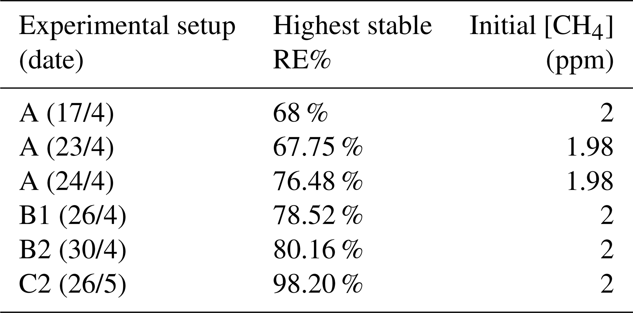
The system yielded an average methane depletion of 86.63 % with a peak depletion at 98.2 %. Various parameters were changed throughout the experiments, and it was determined that the methane depletion is highly dependent on the flow, chlorine production and light source. A better control of these parameters will yield higher and steadier removal of methane.
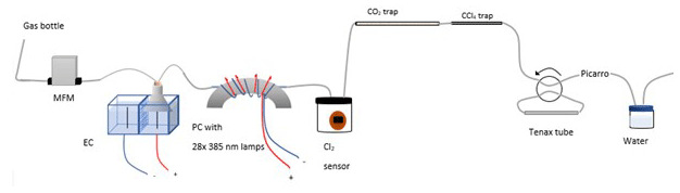
Figure A1Experimental setup B2 with the inclusion of an activated carbon trap. Gas flask: ambient air sample, MFM: mass flowmeter, EC: electrolytic device, PC: photochemical device.
The experimental setup B2 is presented in Fig. A1.
A1 The electrolytic device
The experimental setups presented in Table A1 use an electrolytic device to produce chlorine gas. The electrolytic device is housed in a polycarbonate box. A Nafion membrane (Chemours, Nafion N234) is installed, dividing the volume into two half-cells. Two electrodes are installed, and the two cells consist of two different solutions of NaCl in Milli-Q water. The average concentration of NaCl is 1.3 M at the anodic site and 0.13 M at the cathodic site. The electrodes are carbon electrodes with a diameter of 2 mm and a length of 10 cm. On the anodic side Cl2 is produced (Pletcher and Walsh, 2012).
Anode reaction:
Cathode reaction:
Overall reaction:
The presence of the membrane is essential due to its selectivity to cations. The membrane allows Na+ ions move from the anode to the cathode and form NaOH. If the membrane was not present the NaOH would encounter Cl2 and form hypochlorite.
A2 The electrolysis chamber
In the experimental setups A to B2 (Table A1), an electrolysis chamber is used to generate Cl2; see Fig. A1. The chamber is made from PVC plastic; 28 LED (385 nm; UV LED LAMP-VAOL-5EUV8T4) diodes were installed in the chamber, directed at a quartz tube (o.d. 4 mm, length 20 cm) placed through the chamber. The LEDs are connected in parallel with a forward voltage and forward current. The max current is 20 mA for each LED, and the max voltage is 3.6 V. The same voltage runs through the LED and the current is multiplied by the number of lamps, resulting in 0.480 Å.
The chlorine gas is introduced into the gas stream by using a funnel above the anode. The water level is adjusted to yield optimal conditions for Cl2 to get into the gas stream and avoid chlorine being deposited on the water surface or water getting sucked into the gas stream.
A3 Additional equipment
The Picarro G1301 has a cavity pressure of 18.7 kPa, nominal ambient temperature (DAS temperature) of 30.2 ∘C and cavity temperature of 45 ∘C.
We used a cylinder of compressed air with stable mole fractions of CH4 (1.98 ppm), CO2 (376.1 ppm) and H2O (1.175 % vol).
The Cl2 sensor used in all experiments is the PG610-CL2 model, which is a chlorine Cl2 gas detector with a gas sound light vibration alarm. The sensor measures chlorine concentrations from 1–20 ppm. The sensor is placed in a 600 mL glass flask.
The general procedure is as follows.
-
Prepare solutions.
-
Let the system stabilize.
-
Turn on the electrochemical device.
-
Let the Cl2 concentration stabilize.
-
Turn on lamps.
-
Let the system stabilize to ensure a stable RE%.
-
Take a 10 min measurement with Tenax tube sampling (experiments B1 and B2).
-
Turn off the light.
-
Let the system stabilize to the initial methane concentration.
A4 Variations in the experimental setups
Experimental setup A is the initial setup. Experimental setup B1 employed Tenax tube sampling for thermal desorption–gas chromatography mass spectrometry (TD-GCMS) measurements of chlorinated species.
Experimental setup B2 follows the same procedure as B1, but with the addition of an activated carbon trap.
Experimental setup C1 uses a high-pressure xenon lamp (ILC Technology R100-IB). The xenon lamp lights up the second photolysis chamber (PC-2), which is equipped with an 8 mm diameter and 20 cm length quartz tube. The inner surface of the cylinder is covered with aluminum foil to reflect the light coming in. The xenon lamp emits light in wavelengths from vacuum UV (200 nm) to infrared (Moore et al., 2009); therefore, a 335 nm optical filter is installed.
At the Picarro G1301 outlet the two traps are used for trapping the gases hydrochloric acid, chlorine gas and carbon dioxide.
Experimental setup C2 is similar to C1; however, the Cl2 concentration is diluted to obtain values above the fixed value of 20 ppm. At the electrochemical device outlet a union tee divides the flow into two channels, one to the PC-2 and the other to the sensor chamber. The flow at the outlet of the sensor chamber is measured by a flowmeter (Agilent ADM) to ensure a flow of approximately 40–50 mL min−1.
The photochamber for the high-pressure xenon lamp (HPXL) setup uses a quartz tube with dimensions 20 cm in length and in. (12.7 mm) in outer diameter placed in a cylinder coated with aluminum.
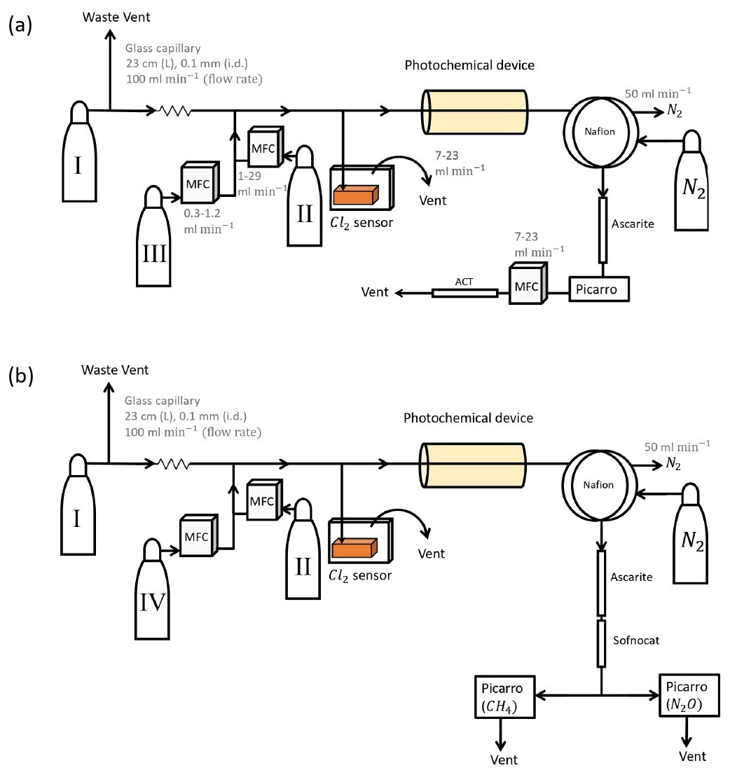
Figure B1(a) General setup for setups 2–4 (Table D4). (b) General setup for N2O experiments. Gas flasks are presented in Table B1. ACT: activated carbon trap. MFC: mass flow controller.
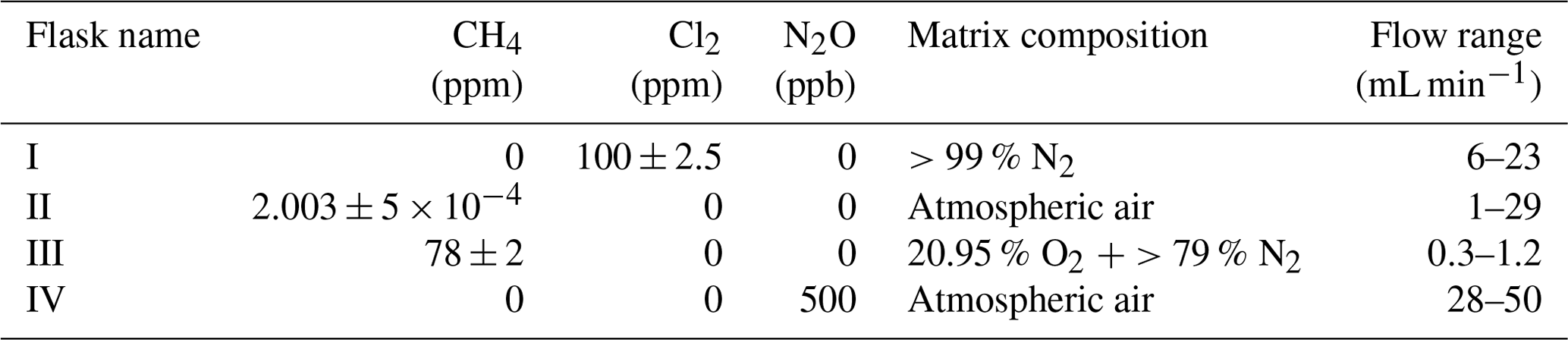
Table B1Table summarizing the gas flask used in the experiments.
The photochemical device (PD; Fig. B2) for later experiments (Fig. B1) consists of 420 LEDs at 365 nm peak wavelength. The LEDs run in a parallel circuit with a forward voltage and forward current (from positive to negative). The max current is 13.2 mA for each LED, and the max voltage is 3.8 V. The same voltage runs through the LEDs, resulting in a total current across the system of 5.5 A.
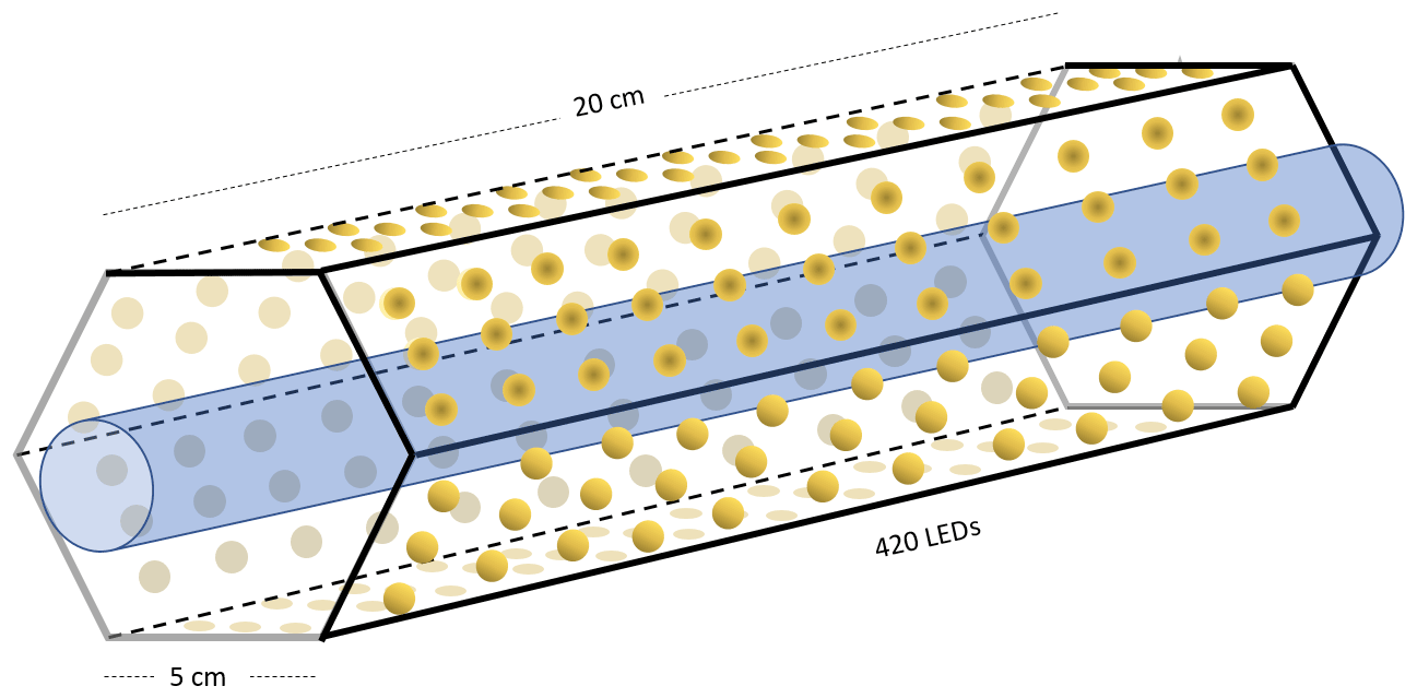
Figure B2Hexagonal photochemical device consisting of connected circuit boards of 420 LEDs at 365 nm.
The difference between the two similar setups 2 and 3 is that the forward pressure valve is exchanged with a mass flow controller to allow for a smaller and more stable level of vent flow. The quartz tube of the previous experiments is substituted with seven smaller quartz tubes for setup 4 to yield a longer tR.
B1 Experimental procedure
-
Tune the desired flow from flask C for methane and mix it with a flow from flask B equal to the desired flow plus the intended flow from flask A.
-
Let the system stabilize.
-
Add the desired flow of chlorine from flask A by adjusting the pressure at the flask.
-
Reduce the flow from flask B by an equal amount to get the desired mixing ratio.
-
Let the system stabilize and confirm that the resulting total flow fits the expected flow. Make sure the chlorine value can be read on the chlorine sensor.
-
When a stable methane level has been run for sufficient time, turn on the photochemical device.
-
Let the system stabilize to ensure a stable methane RE%.
-
Turn off the light.
-
Let the system stabilize to the initial methane concentration before the light is turned on.
B2 N2O experiments
Experiments were conducted with the Picarro model G5131-i, which is used to measure N2O mixing ratio and isotopic abundance. The purpose of the experiments was to confirm that the illumination did not affect N2O. The general experimental setup is shown in Fig. B1b. The sofnocat trap was prepared with 1.25 g of sofnocat contained in a 6.4 mm diameter tube of length 8 cm and kept in place by glass wool. The trap was installed to prevent effects on the N2O isotope signal from CO, as presented in Harris et al. (2020). The presence of CO 1 ppm gives rise to an erroneous offset in the observed isotopologue values of 1.2, 2.4 and 0.4 ‰ for δ15Nα, δ15Nβ and δ18O, respectively. The installation of this trap after the CO2 trap allowed us to measure the amount of CO present. The technical air from flask C was exchanged with a technical air mix with 509 ppb [N2O], allowing for dilution to the ambient level. The flow ratio between the three different gases was regulated to maintain a mixing ratio of 330 ppb N2O, 2.4 ppm CH4 and 33 ppm Cl2. Power supply to the lamp was constant at 4.8 V and 5.0 A, and tR in the chamber was varied between 86, 117 and 145 s.
The model is made with the program Kintecus version 6.8 (Ianni, 2012). The model was developed by describing the relevant reactions with rates for chlorine radical production and/or removal as well as formation of chlorinated species. The model was kept as simple as possible while still including key reactions. The reactions and their rates used in the model are found in Tables E1–E3. A simplified reaction scheme is shown in Fig. 2. The experiments are modeled by choosing both the initial and external concentrations of the species used and the tR within the chamber. A continuous flow was modeled by setting the initial and external concentrations of gases flowing through the chamber to the same value. This is done for the gases Cl2, CH4, N2 and O2.
The physical parameters are fixed as well: temperature at 298 K, starting integration time to 10−6 s (starting step for the integrated model), maximum integration time to 1 s, simulation length equal to tR plus 5 s and the accuracy of digits to 10−4. Furthermore, the energy unit kilocalorie (kcal) was selected, and the unit of concentration was selected to be molecules per cubic centimeter ().
C1 Radical wall reactions
As described in the main article a set of radical-terminating reactions was incorporated into the model. The wall reaction rates were estimated based on the diffusion rate of the radicals and the diffusion length. The diffusion length is calculated as the average distance from the wall. Because two different sizes of tubes were used throughout the experiments, the wall reactions reflect that. The diffusion length and the diffusion rate are given in Eqs. (C1) and (C2), respectively:
where D is the diffusion constant and t is time.
The distance, l, is defined as the average distance from the wall, which can alternatively be written as , where r is the radius of the tube, and dc is distance from a random particle in the cylinder to the center of the circle of the cylinder. Finding the average distance to the wall of an infinite number of randomly located particles in the cylinder can be accomplished by solving Eq. (C3). The result of Eq. (C4) is used to calculate the resulting diffusion rate with the inclusion of the average distance from the walls of the tube, which is defined in Eq. (C5).
Here, r is the radius and is the area.
The diffusion constants, diffusion lengths and estimated wall reaction rates are shown in Table E3.
Judeikis and Wun (1978)Seinfeld and Pandis (2016)Ivanov et al. (2007)Ivanov et al. (2007)Table C1Radical wall reaction parameters.
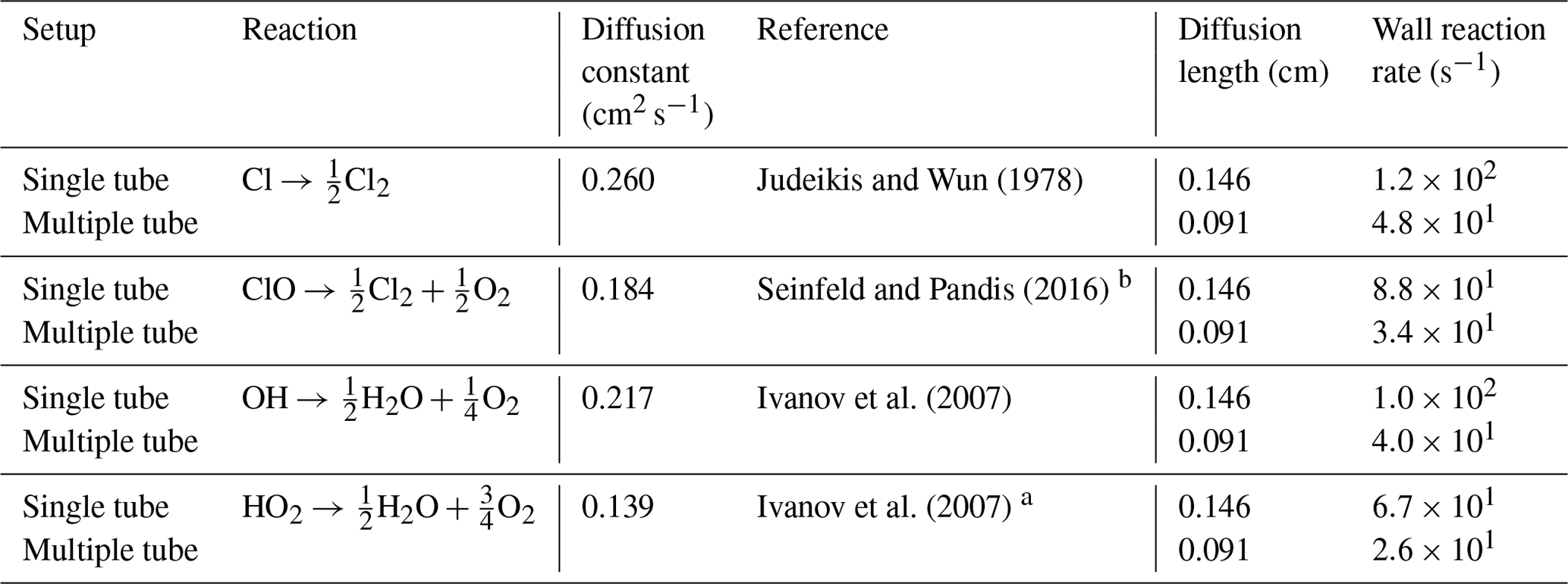
a The diffusion coefficient is estimated from DHO−Air and . b The Chapman and Cowling (1939) diffusion model was used to estimate the diffusion constant.
C2 estimation
C2.1 First approach
The first approach is to fit in the model to regenerate the observed removal efficiencies from experimental results. These fits were only produced for experiments investigating the effect of Pin. The resulting was related to Pin via the effective power-to-light conversion based on the absorption cross section of Cl2 and the wavelength distribution of the LEDs. was determined in this manner, once for the single-tube systems and once for the multiple-tube systems. The photolysis rate J (photons−1) can be determined by Eq. (C6):
where σ(λ,T) is the wavelength-dependent cross section of Cl2 (cm2 molec.−1), ϕ(λ,T) is the quantum yield and I(λ,W) is the spectral actinic flux density (photons cm−2 s−1 nm−1). The cross section of chlorine dissociation in the range 250–550 nm is defined by Eq. (C7) (Burkholder et al., 2020).
Here, T is the temperature, and λ is the wavelength (nm).
The actinic flux (Eq. C8) is a function dependent on the power output P(λ,W) from Eq. (C9), the distribution D(λ) from Eq. (C11) and the tube volume (V):
where h is Planck's constant, and c is the speed of light.
It was observed that the photolysis rate did not scale linearly with the applied power, which we speculate may be due to variation of the efficiency of the lamp with the applied current and operating temperature. This effect was sufficiently accounted for by a linear fit and is defined as Eff (W):
where W is the power supplied to the diodes, and values for the constants a and b are fitted in the model to match the experiment. The function (C10) accounts for additional variations such as effects due to temperature, the cross-sectional area of the quartz tube, the conductance of the photochamber and the quality of the distribution fit. This is reflected in the constants a and b varying in response to changes in these parameters. As this is used as a simple empirical stand-in function we do not intend to speculate further on how these changes change the constants.
The photon output (Eq. C9) from the LED was assumed to follow a normal distribution. For this distribution shown in Eq. (C11), we assumed a center value of 365 nm and full width at half-maximum of 10 nm. The distribution (Eq. C11) is per nanometer (nm−1).
The photolysis rate could then be calculated by Eq. (C6) across 250–500 nm at 298 K.
C2.2 Second approach
A second approach for estimating and relating it to PIN was used. This method estimated by using simplified kinetics and relating it to power via the same method as the model-derived . Exp. F reflects the single-tube system, while exp. I reflects the optimized multiple-tube setup. Four main reactions, (CR1)–(CR4), are considered in the simple kinetic model.
The Cl radicals are consumed at a fast rate; therefore, a steady-state approximation for Cl has been assumed.
The photolysis rate for the kinetic calculation is thereby defined in Eq. (C13).
The photolysis rate is calculated from an estimated [Cl] concentration. This was achieved by assuming that the methane concentration would follow an exponential decay with time (Eq. C14). The estimated [Cl] is expressed in Eq. (C15):
where [CH4]t is the methane concentration at time t, while [CH4]0 is the initial concentration.
The values for Jkin are generated by inserting the experimental values of [Cl2], [CH4] and the estimated value of [Cl] into Eq. (C13).
The distribution function D(λ) from Eq. (C11) can be used in combination with the cross section to determine the scale factor Jscale.
The value of Jscale is calculated from the overlap integral between σ(λ,T) and the emitted photon distribution.
The variable l is the path length across the tube(s) in centimeters (cm), and V is the volume of the tube(s) (mL). λ is the wavelength (nm), h is Planck's constant and c is the speed of light. Values for the constants a and b from Eq. (C17) are then fitted to match the photolysis rate in Eq. (C18) with the photolysis rate found from the Kintecus model.
Here, Peff is the effective power, and the constants a and b are setup-dependent constants.
From the effective power output the photolysis rate could be calculated by multiplying Peff with Jscale.
C3 fitted to collected data
The is fit to the data collected for some of the experimental steps for exp. F and I to determine the values for the constants a and b.
Exp. F is the single-tube system and exp. I is the optimized multiple-tube system. From the fitted a, b and calculated Jscale the photolysis rate could be calculated for the other experiments.
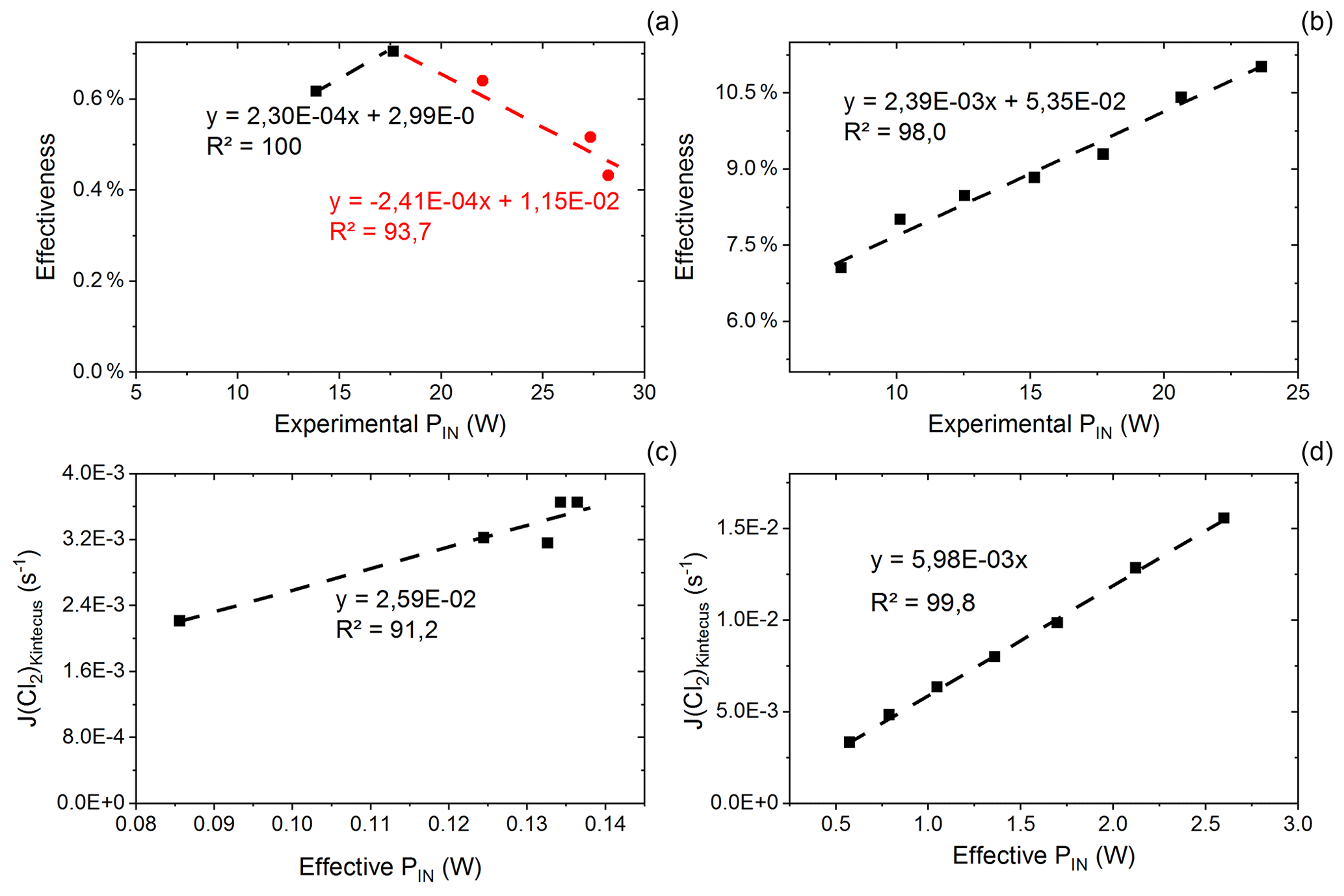
Figure C1(a) Effectiveness as a function of experimental power input for exp. D. The correlation is used for calculating the effective PIN for single-tube experiments. (b) Effectiveness as a function of experimental PIN for exp. I. The correlation is used for calculating the effective power for multiple-tube experiments. (c) Kintecus-obtained as a function of the effective pIN for exp. D. The effective pIN is calculated from Fig. C1a. The combination of the figure with Fig. C1a is used to calculate the for single-tube experiments by Eqs. (C19) and (C20). (d) Kintecus-obtained as a function of the effective pIN in exp. I. The effective pIN is calculated from Fig. C1b. The combination of the figure with Fig. C1b is used to calculate the for multiple-tube experiments by Eq. (C21).
C3.1 Single-tube systems
values are generated on the basis of exp. D2 and D6–D9. The efficiency of pIN is generated from the model. A correlation between effectiveness (%) and experimental pIN (W) is shown in Fig. C1a as is the correlation with the (Kintecus) values in Fig. C1c.
The dependence on the pIN (W) for the single-tube system in exp. B, C and D is given by Eqs. (C19) and (C20). The equations incorporate a decrease in efficiency of pIN at higher levels due to overheating of the chamber as seen in Fig. D2c.
The comparison between modeled and experimental efficiency for the single-tube experiments is seen in Fig. E1a and b.
C3.2 Multiple-tube systems
is generated in the same manner as the experiment for results with multiple tubes. Here exp. I is used to obtain model values (Fig. C1b and d).
The overheating at high pIN is eliminated with the improved photochemical device. This is also apparent when comparing the effectiveness, which is approximately 9 % for the multiple-tube configuration (Fig. C1b) and approximately 0.6 % for the single-tube system (Fig. C1a) at the same pIN of 15 W. Figure E1e and f show the comparison for exp. G and H, respectively.
C3.3 Exp. E and F
Some experiments cannot be related to the relations presented for the single- and multiple-tube systems. This is due to the optimization done on the photochemical device. A second approach with additional kinetic calculations is therefore used to estimate the of these two experiments. The effectiveness of exp. E is shown in Eq. (C22).
In the same manner, the effectiveness of exp. F in shown in Eqs. (C23) and (C24).
D1 CH4 experimental results
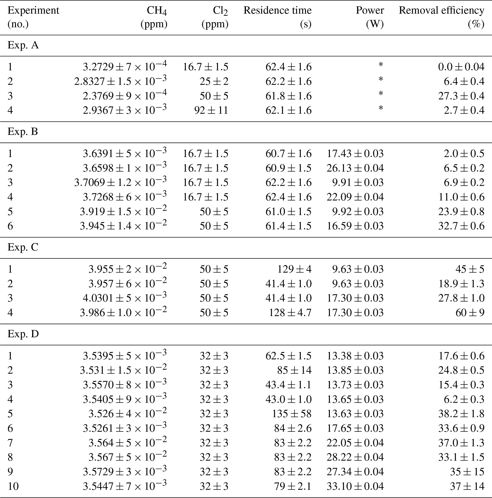
In Tables D1–D3 the four varying parameters [CH4]initial, [Cl2], tR and PIN are presented for each experiment alongside the resulting RE%. Table 4 summarizes the experiments done in the study.
Table D1Data for exp. A–D. Columns: experimental steps, [CH4] (ppm), [Cl2] (ppm), residence time tR (s), power input pIN (W) and the resulting removal efficiency in %.
* The pIN of the xenon lamp was not varied or determined.
Table D2Data for exp. E–F. Columns: experimental steps, [CH4] (ppm), [Cl2] (ppm), residence time tR (s), power input pIN (W) and the resulting removal efficiency in %.
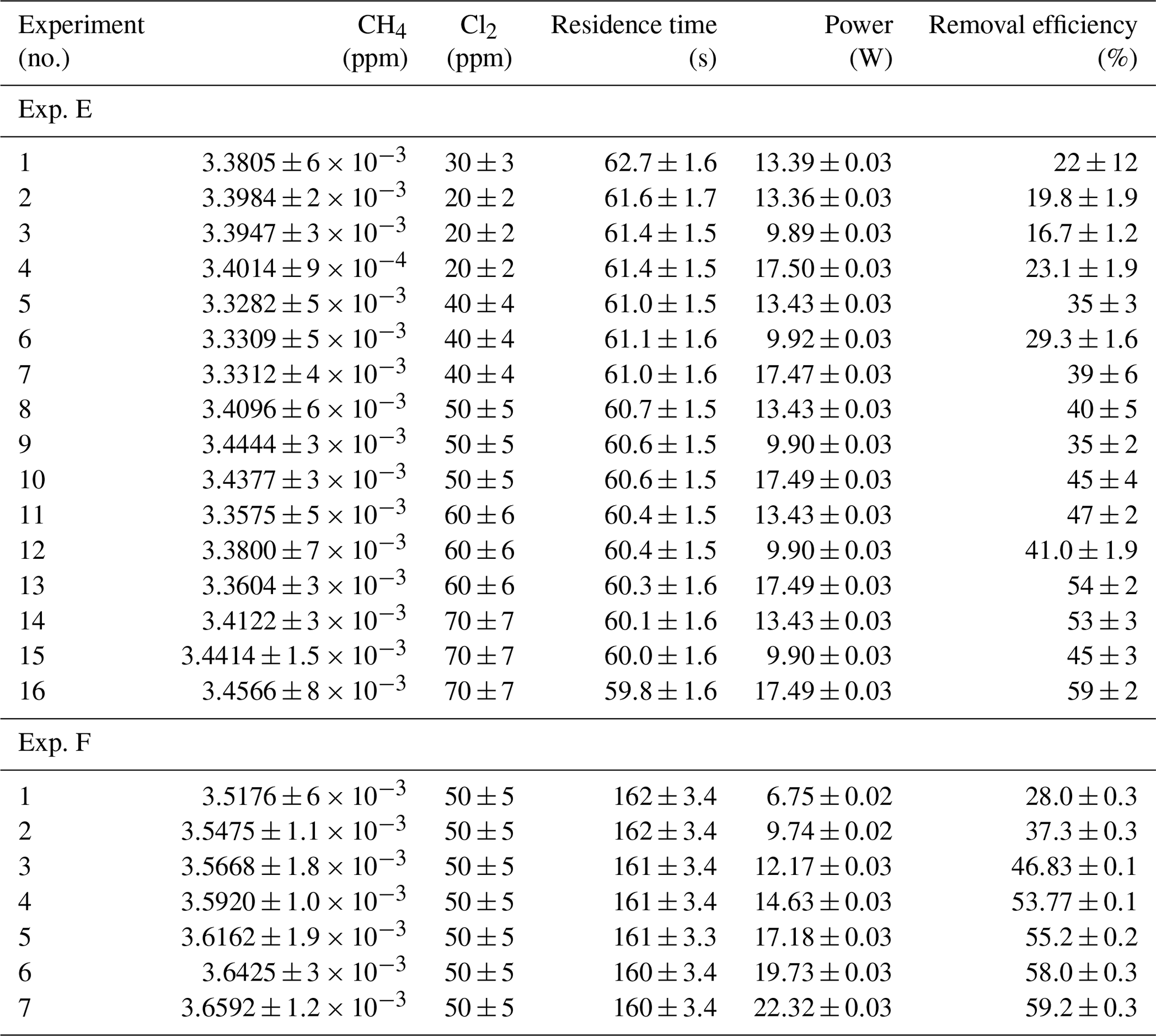
Table D3Data from exp. G–I. Columns: experimental steps, [CH4] (ppm), [Cl2] (ppm), residence time in seconds, power in watts and the resulting removal efficiency (%).

* The [CH4] values are calculated based on trend fitting.
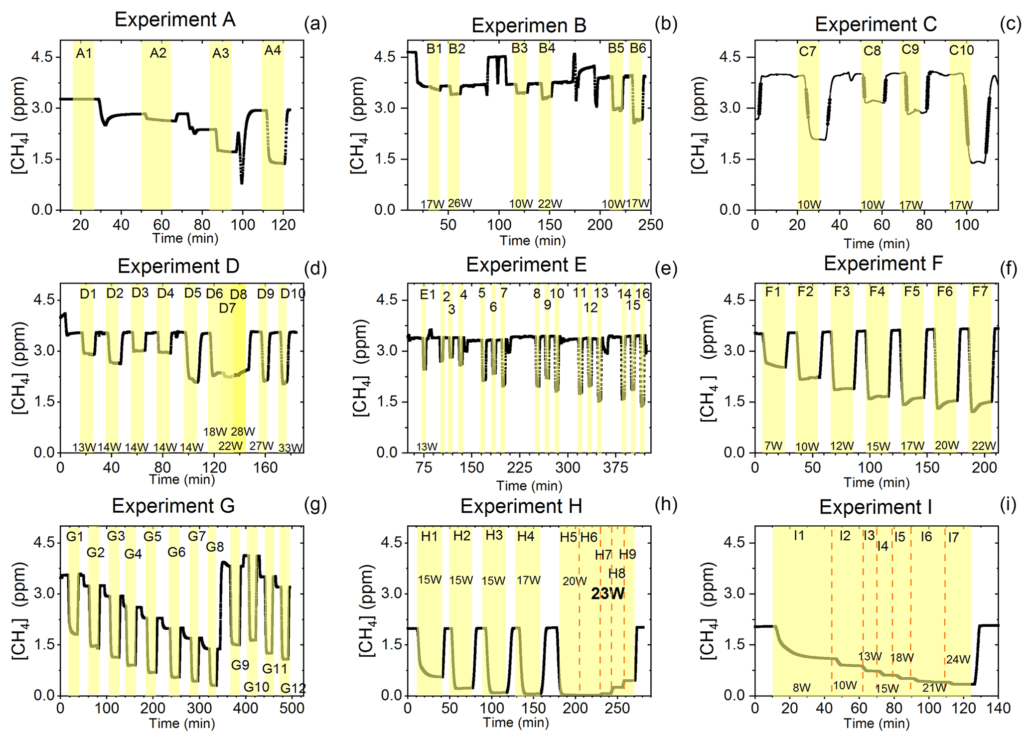
Figure D1Exp. A–I are shown. Each illuminated step has been highlighted. (a) The CH4 is seen as a function of time. The [Cl2] is varied. (b) The light intensity and [Cl2] are varied. (c) Steps 7–10 highlighted. The light intensity and tR are varied. (d) Steps 1–10 are highlighted. The light intensity and tR are varied. (e) Steps 1–16 are highlighted. The light intensity and [Cl2] are varied. Following the initial illumination at 13 W the sample was illuminated at three different pIN for five different chlorine concentrations. The pIN was of the order 13, 10 and 17 W with chlorine steps 20, 40, 50, 60 and 70 ppm. (f) Steps 1–7 are highlighted. The light intensity is varied. (g) Steps 1–12 are highlighted. The CH4 level is varied, while the light intensity is kept the same. (h) Steps 1–9 are highlighted. The light intensity and tR are varied. (i) Steps 1–7 are highlighted. The light intensity is varied. Prolonged and stable photolysis was enabled due to cooling. Increasing levels of pIN for the photochemical chamber define the seven different steps.
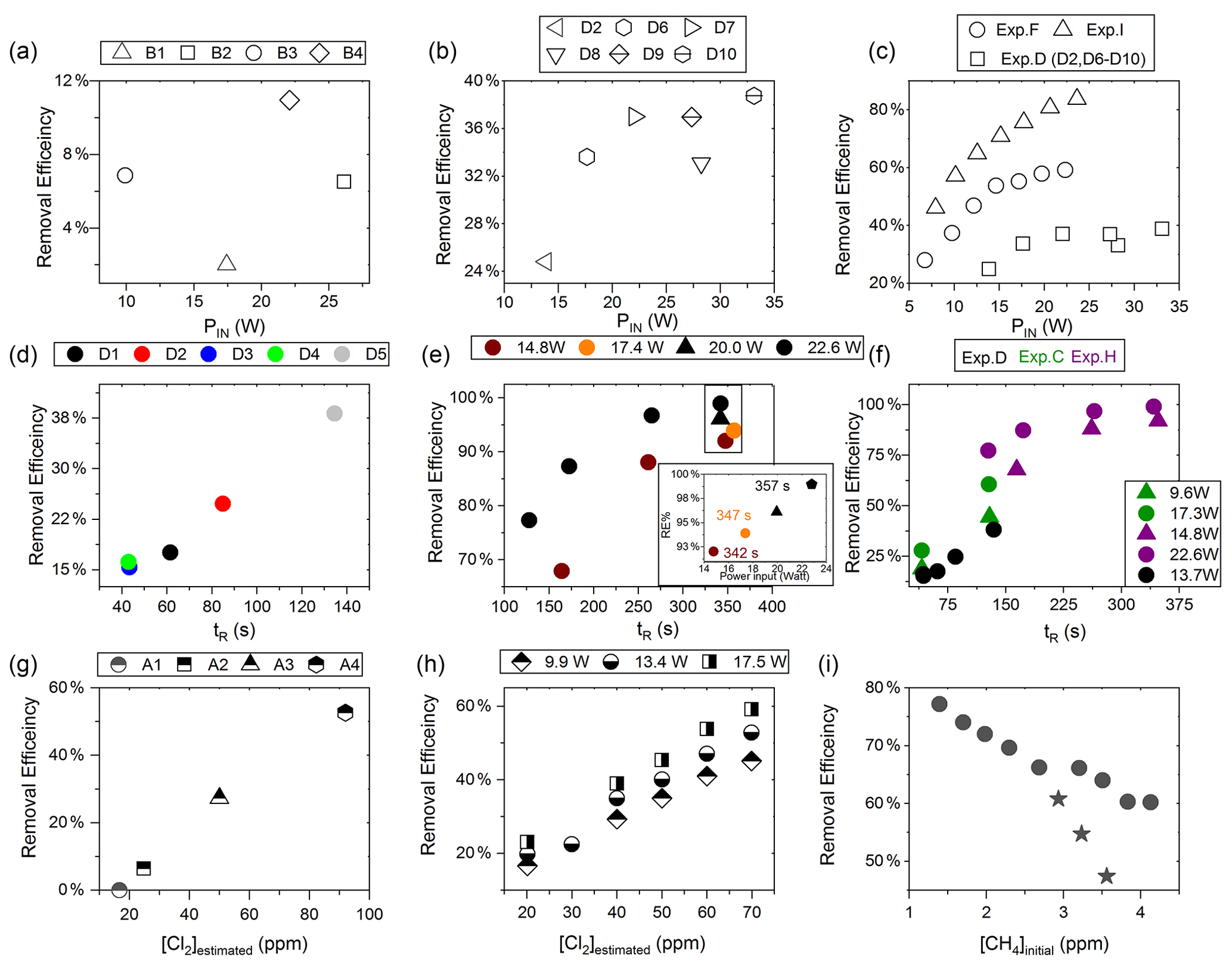
Figure D2(a) RE% as a function of pIN for exp. B1–B4. (b) Experiment steps D2 and D6–D10: RE% as a function of pIN (W). (c) RE% of methane plotted against pIN (W). The results from three experiments, D (square), F (circle) and I (arrow), have different settings in tR, [CH4] and [Cl2]. (d) Experimental steps D1–D5: tR (s) in the photochemical device as a function of tR in seconds. (e) The resulting removal efficiencies of exp. H plotted against tR. An additional zoom inset on the four points around 350 s reveals the removal effect plotted against power. (f) RE% of methane plotted against tR in seconds. The results from three experiments, D (black), C (green) and H (purple), have different settings in pIN, [CH4] and [Cl2]. (g) RE% as a function of [Cl2] (ppm) for the xenon lamp in exp. A. (h) Resulting RE% plotted against [Cl2] (ppm) for exp. steps E2–E16. Three different power settings are used: 9.9 W (diamond), 13.4 W (circle) and 17.5 W (square). (i) The RE% is displayed as a function of the initial methane concentration with the remaining fixed parameters such as Cl2 mixing ratio, tR and pIN. The three points (star) in the figure represent steps suffering from early experimental deviation.
Table D4Table summarizing experiments and setups. FC: flow-controlled, PC: pressure-controlled, CWL: chlorine waste line.
D1.1 Setup 1 (HPXL) experiments
The xenon lamp experiments shown in Fig. D1a were performed to confirm that the Cl2 added to the gas mix could make it to the photolysis chamber. The RE% of methane was found as a result of varying the [Cl2] to 16.7, 25, 50 and 92 ppm as seen in Fig. D2g. Each concentration step was given 10 min to stabilize before the xenon lamp was turned on for 10 min. The gas provided to the system was a dynamic mix of flows from three different flasks (see Table B1). Due to this, it was possible to vary the abundance of chlorine while keeping [CH4] constant. The experiment confirmed that the level of Cl2 could be controlled and that higher levels resulted in greater depletion of methane.
D1.2 Setup 2 (single-tube, flow-controlled chlorine waste line) experiments
In exp. B, PIN was varied in steps 1 to 4, as presented in Fig. D1b. The aim was to determine the effect of varying light intensity. Figure D2a shows the RE% as a function of pIN for experiments 1 to 4. The initial methane concentration is maintained at 3.68±0.02 ppm. Steps 1 and 2 are both examples of the start-up deviation. At the time of steps 3 and 4, sufficient flushing had taken place.
Table D5Exp. B. The three experimental steps clearly show an increasing RE% as the pIN and the Cl2 mixing ratio are increased.

The chlorine concentration was increased from 16.7 to 50 ppm starting with step 5. The four relevant variables and resulting RE% can be seen in Table D5. [Cl2] was increased by a factor of 2.5 between steps 3 and 5. The increase results in a 3.5-fold increase in RE%. Furthermore, the pIN is increased when going from step 5 to 6, which also leads to an increase in RE%. In a comparison between these three steps, the positive relation for both chlorine concentration and pIN to the RE% was confirmed.
D1.3 Setup 3 (single-tube, pressure-controlled chlorine waste line) experiments
Three experiments (C, D and E) used this setup. Exp. C presented in Fig. D1c was carried out with a constant supply of [Cl2] at 50 ppm and [CH4] at 3.981±0.018 ppm. Steps 2 and 3 had the same tR as steps 1 and 4. In addition, the experiments vary in pIN, as can be seen in Table D6. Table D6 shows how the combination of increased tR and pIN yields a higher RE%.
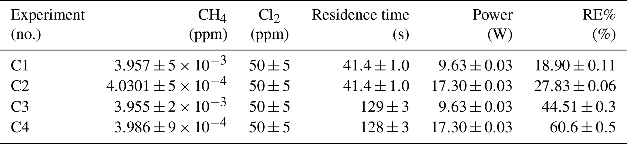
Exp. D was carried out with [Cl2] kept constant at 32 ppm. The initial methane concentration was maintained at 3.547±0.005 ppm. Similarly to exp. C the tR and pIN were varied. Steps 1 to 5 are carried out with the same pIN in the device but with varying residence times; see Fig. D2f and d. In Fig. D2f the data for exp. D exhibit clear agreement between tR and RE%. The longer tR within the photochamber results in greater removal efficiencies. Steps 2 and 6–10 are carried out with the same tR but with varying pIN; see Fig. D2c and b.
The experimental steps of exp. E (Fig. D1e) were held at the same initial methane concentration of 3.39±0.01 ppm and the same tR of 60.82±0.18 s. Throughout the experiments, three levels of pIN were tested against varied levels of Cl2 mixing ratio spanning in the range 20–70 ppm. Figure D2h presents, looking at 20 ppm Cl2, the fact that a greater pIN yields higher RE%.
D1.4 Setup 4 (multiple-tube, pressure-controlled chlorine waste line) experiments
Four experiments (F, G, H and I) were done with this setup. Exp. F (Fig. D1f) was run at a constant level of [CH4]initial at 3.593±0.019 ppm and [Cl2] at 50 ±5 ppm. At a flow kept at 15.5 mL min−1 the tR in the photochamber was maintained at 161.06±3 s. Across exp. F stepwise changes were made for pIN ranging from 6.75–22.92 W. The daily measurement is presented in Fig. D1f, where the removal for the steps, with the exception of the first step, is characterized by an initial RE%, but this efficiency drops during the first 5 min of illumination. The relationship found between removal and pIN for exp. F can be seen in Fig. D2c.
Exp. G was carried out with a stepwise change in [CH4]inititial in the range 1.39 to 4.13 ppm at constant tR of 164 s, [Cl2] of 50 ppm and pIN of 14.6 W. The daily result can be seen in Fig. D1g, where the improvement of silicone removal can be observed from stable levels of RE%. As can be seen in Fig. D2i decreasing the initial methane concentration yields, as expected, a greater RE%.
Exp. H was carried out with the constant [CH4]inititial at 2.000±0.003 ppm and Cl2 mixing ratio at 50±5 ppm, but with mixed settings of tR and power. Steps H1–H3 were done with constant power at 14.8 W with tR increasing from 164–350 s. Then, keeping tR around 350 s, three steps of increasing power were tested ranging from 14.8–22.8 W. Between steps H4 and H5 a fan was installed. The final three steps were kept at 22.8 W and stepped through reduced tR from 342–130 s.
Exp. I was carried out with [CH4]inititial maintained around 2.01±0.01 ppm, [Cl2] at 50 ppm and the tR held at 163.1±0.4 s. The only parameter varied was the pIN to the photochemical device. The light was turned on at 7.9 W and was left on for the duration of the experiments with a stepwise increase in PIN after stable removal had been maintained for 5 min. The resulting methane concentration can be seen in Fig. D1i. [CH4] increases throughout the experiments due to the chlorine pressure decline. For the purpose of calculating RE%, the expected [CH4] for each of the steps was fitted from the initial [CH4] and the end [CH4]; . The relative median values of initial methane and tR were chosen in order to best resolve the effects of varying pIN. As the removal effect approaches 100 % asymptotically, the sensitivity to changes will be greater at lower removal values.
The results presented for exp. I in Fig. D2c can be compared to the results from exp. D and F and represent the improvements implemented to the system. Unlike for those experiments, the trend of exp. I is explained by one trend asymptotically approaching 100 % removal.
D1.5 Comparison
Figure D2c shows a comparison of three different experiments in which pIN was varied. When comparing experiments F and I the improvement in performance of the device is clear. However, even if tR and [Cl2] are identical, the initial methane concentration of exp. F is 3.59 ppm compared to exp. I at 2.096 ppm. Exp. D alone shares some PIN levels and is operated at the same initial methane level as exp. F. The tR and [Cl2] are lower and less removal is accordingly expected. Hence, the main thing to observe is behavior at higher PIN. The efficiency of the photochamber decreases as seen in exp. D and F. The improvements done on the photochamber and installation of a fan to cool the photochemical chamber have prolonged the lifetime of the chamber and improved efficiency.
Figure D2f shows a comparison of three different experiments in which tR was varied and in some cases PIN as well. tR is improved because the MTH-PD setup made it possible to obtain higher tR and more efficient use of the photochemical chamber. The experiments with a single tube do not have long residence times. As seen in Fig. D2f longer tR greatly improves the RE% and is therefore essential to further improve the setup.
D2 N2O experimental results
From the experiment investigating the compatibility of the removal method and the analysis of N2O, it was found that the oxidization had no effect on the N2O abundance or the isotopic composition. It was, however, discovered that the oxidation path for CH4 terminated at CO, as the isotopic signal changed, matching the interference of CO. To remove this effect a sofnocat trap was implemented, which oxidizes the CO to CO2. By applying the trace gas and matrix corrections described in Harris et al. (2020), it was found that the isotopic levels remained stable across the oxidation. Variation observed in the N2O was due to the unstable supply of Cl2, resulting in slight shifts in the dilution. The values of δ15Nα and δ18O were both found to approach the unaffected target value during the oxidation as was hoped. Results are shown in Fig. D3

Figure D3Results from the three experiments J, K and L using the G5131-i for N2O isotope measurements. The CH4 level is depicted in each row (ppm) along the first y axis. Highlights indicate the several different oxidation settings. Row 1: measurements of δ15Nα (‰) plotted along the second y axis. Red highlights a 100 s average measured value corrected for O2, CO and CO2 effects, while grey indicates a 100 s average value that has been corrected for all interference including CH4. Row 2: measurements of δ15Nβ (‰) plotted along the second y axis. Red highlights a 100 s average measured value corrected for O2, CO and CO2 effects, while grey indicates a 100 s average value that has been corrected for all interference including CH4. Row 3: measurements of δ18O (‰) plotted along the second y axis. Red highlights a 100 s average measured value corrected for O2, CO and CO2 effects, while grey indicates a 100 s average value that has been corrected for all trace gas interference including CH4. Row 4: measurements of [N2O] (ppb) shown in blue. Variation observed corresponds to fluctuations in the mixing of the three gases. Exp. J: in this experiment the light was turned on throughout the entire experiment, with the experimental steps corresponding to changes in tR. Exp. K: in this experiment two experimental steps were used with different power settings. Exp. L: in this experiment the sofnocat trap was used in the first three experimental steps, while steps 4 and 5 were completed without. The variation between experimental steps corresponds to changes in tR.
The results from the kinetic model are shown in Fig. E1.
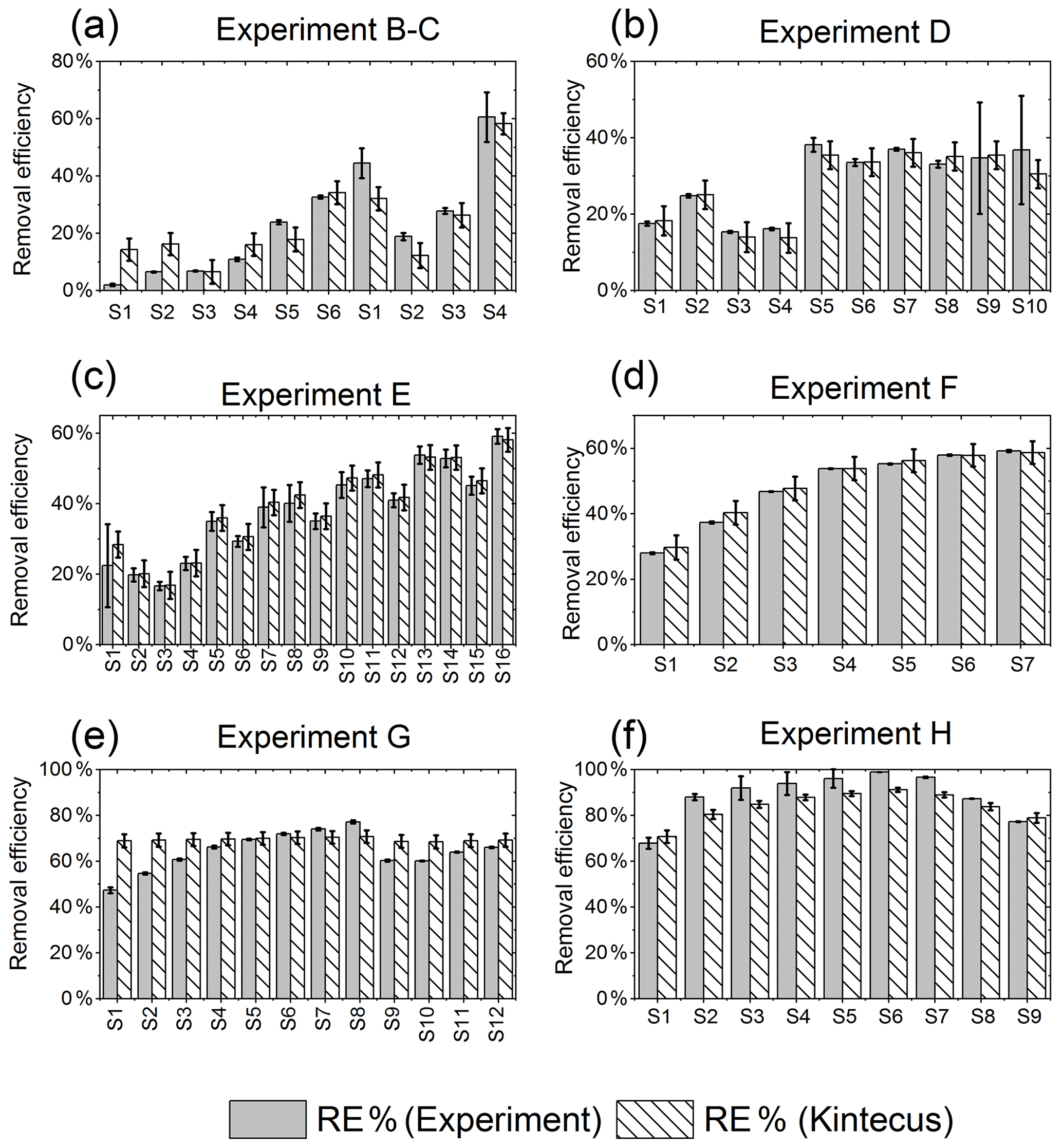
Figure E1RE% as found experimentally (grey) and by the model (white stripes). (a) Exp. B and C, (b) exp. D, (c) exp. E, (d) exp. F, (e) exp. G, (f) exp. H.
Table E1JPL: Burkholder et al. (2020). Hossaini: Hossaini et al. (2016).
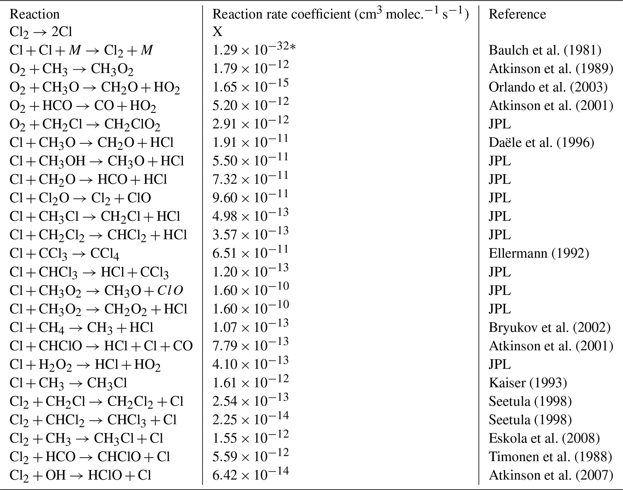
* Third-order rate expression (units cm6 molec.−2 s−1).
Table E2JPL: Burkholder et al. (2020). Hossaini: Hossaini et al. (2016).
* Third-order rate expression (units cm6 molec.−2 s−1).
Table E3JPL: Burkholder et al. (2020). Hossaini: Hossaini et al. (2016).
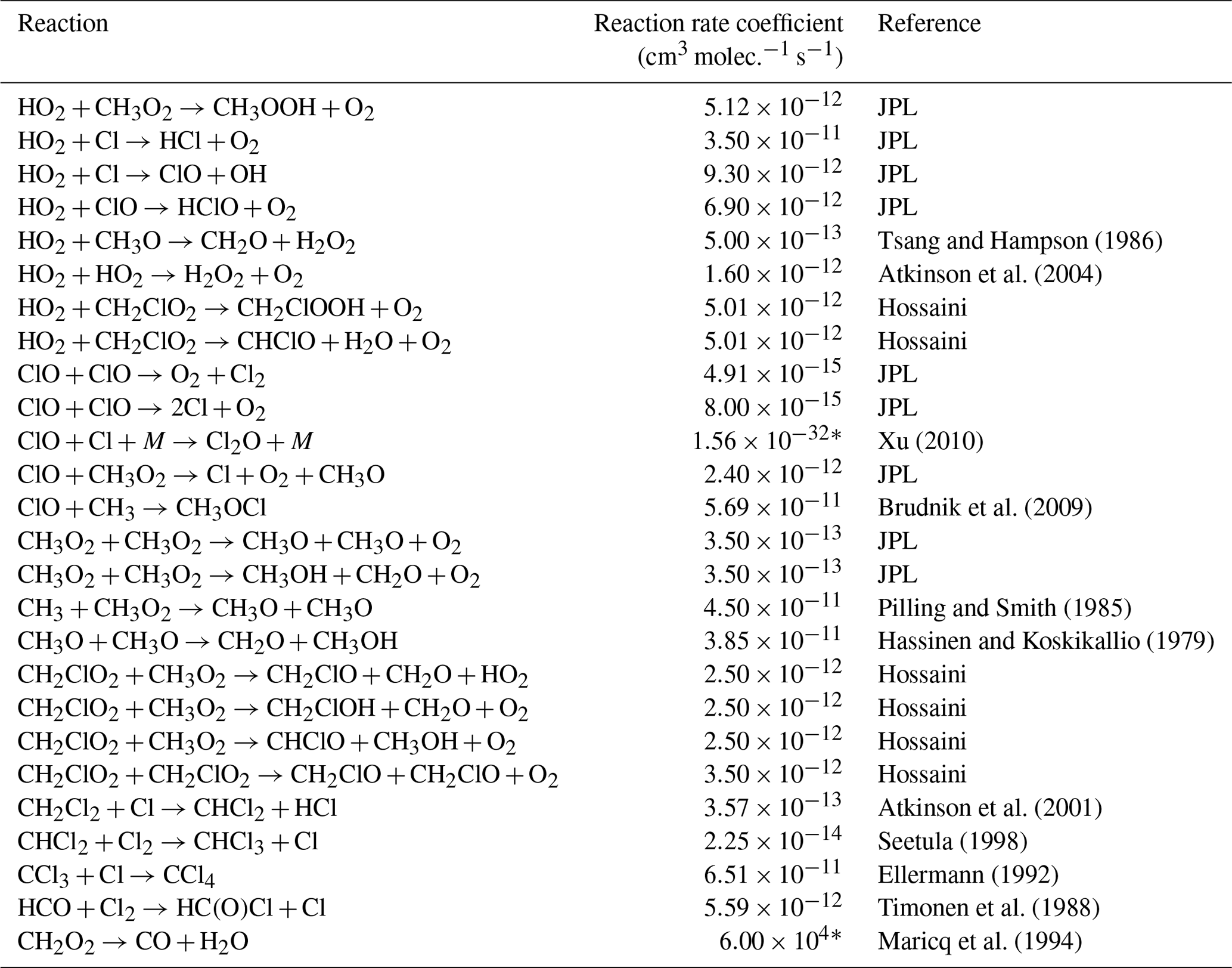
* Third-order rate expression (units cm6 molec.−2 s−1).
All data are available from the corresponding author upon request.
MSJ, MP and JBL conceived and planned the experiments. MP and JBL carried out the experiments. MP, JBL and MK planned and carried out the simulations. MP and JBL contributed to the interpretation of the results. MP and JBL wrote the paper in consultation with TB and MSJ. All authors provided critical feedback and helped shape the research, analysis and paper.
The authors declare that they have no conflict of interest.
Publisher's note: Copernicus Publications remains neutral with regard to jurisdictional claims in published maps and institutional affiliations.
We thank the Copenhagen Center for Atmospheric Research (CCAR), the Centre for Ice and Climate, and the University of Copenhagen. The authors thank Silvia Pugliese for her help with the reaction mechanism.
This paper was edited by Huilin Chen and reviewed by two anonymous referees.
Atkinson, R., Baulch, D., Cox, R., Hampson Jr., R. F., Kerr, J., and Troe, J.: Evaluated kinetic and photochemical data for atmospheric chemistry: supplement III. IUPAC subcommittee on gas kinetic data evaluation for atmospheric chemistry, J. Phys. Chem. Ref. Data, 18, 881–1097, https://doi.org/10.1063/1.555832, 1989. a
Atkinson, R., Baulch, D., Cox, R., Crowley, J., Hampson Jr, R., Kerr, J., Rossi, M., and Troe, J.: Summary of evaluated kinetic and photochemical data for atmospheric chemistry, IUPAC Subcommittee on gas kinetic data evaluation for atmospheric chemistry web version, 1–56, December 2001. a, b, c, d
Atkinson, R., Baulch, D. L., Cox, R. A., Crowley, J. N., Hampson, R. F., Hynes, R. G., Jenkin, M. E., Rossi, M. J., and Troe, J.: Evaluated kinetic and photochemical data for atmospheric chemistry: Volume I – gas phase reactions of Ox, HOx, NOx and SOx species, Atmos. Chem. Phys., 4, 1461–1738, https://doi.org/10.5194/acp-4-1461-2004, 2004. a
Atkinson, R., Baulch, D. L., Cox, R. A., Crowley, J. N., Hampson, R. F., Hynes, R. G., Jenkin, M. E., Rossi, M. J., and Troe, J.: Evaluated kinetic and photochemical data for atmospheric chemistry: Volume III – gas phase reactions of inorganic halogens, Atmos. Chem. Phys., 7, 981–1191, https://doi.org/10.5194/acp-7-981-2007, 2007. a, b
Baulch, D., Duxbury, J., Grant, S., and Montague, D.: Evaluated kinetic data for high temperature reactions. Volume 4. Homogeneous gas phase reactions of halogen-and cyanide-containing species, J. Phys. Chem. Ref. Data, 10, 129–139, 1981. a
Bonard, A., Daële, V., Delfau, J.-L., and Vovelle, C.: Kinetics of OH radical reactions with methane in the temperature range 295–660 K and with dimethyl ether and methyl-tert-butyl ether in the temperature range 295 618 K, J. Phys. Chem. A, 106, 4384–4389, https://doi.org/10.1021/jp012425t, 2002. a, b
Brudnik, K., Gola, A. A., and Jodkowski, J. T.: Theoretical kinetic study of the formation reactions of methanol and methyl hypohalites in the gas phase, J. Mol. Model., 15, 1061–1066, https://doi.org/10.1007/s00894-009-0461-x, 2009. a
Bryukov, M. G., Slagle, I. R., and Knyazev, V. D.: Kinetics of reactions of Cl atoms with methane and chlorinated methanes, J. Phys. Chem. A, 106, 10532–10542, https://doi.org/10.1021/jp0257909, 2002. a, b
Burkholder, J., Sander, S., Abbatt, J., Barker, J., Cappa, C., Crounse, J., Dibble, T., Huie, R., Kolb, C., Kurylo, M., Orkin, V. L., Wilmouth, D. M., and Wine, P. H.: Chemical kinetics and photochemical data for use in atmospheric studies; evaluation number 19, JPL Publication 15-10, Jet Propulsion Laboratory, National Aeronautics and Space Administration, Pasadena, CA, 2020. a, b, c, d
Chapman, S. and Cowling, T. G.: The Mathematical Theory of Non-Uniform Gases, Cambridge University Press, New York, 1939. a
Cullis, C. and Willatt, B.: Oxidation of methane over supported precious metal catalysts, J. Catal., 83, 267–285, https://doi.org/10.1016/0021-9517(83)90054-4, 1983. a
Daële, V., Laverdet, G., and Poulet, G.: Kinetics of the reactions of CH3O with Cl and CIO, Int. J. Chem. Kinet., 28, 589–598, https://doi.org/10.1002/(sici)1097-4601(1996)28:8<589::aid-kin4>3.0.co;2-r, 1996. a
Ellermann, T.: Fine structure of the CCl3 UV absorption spectrum and CCl3 kinetics, Chem. Phys. Lett., 189, 175–181, https://doi.org/10.1016/0009-2614(92)85119-U, 1992. a, b
Erler, D. V., Duncan, T. M., Murray, R., Maher, D. T., Santos, I. R., Gatland, J. R., Mangion, P., and Eyre, B. D.: Applying cavity ring-down spectroscopy for the measurement of dissolved nitrous oxide mole fractions and bulk nitrogen isotopic composition in awuatic systems: Correcting for interferences and field application, Limnol. Oceanogr.-Meth., 13, 391–401, https://doi.org/10.1002/lom3.10032, 2019. a
Eskola, A. J., Timonen, R. S., Marshall, P., Chesnokov, E. N., and Krasnoperov, L. N.: Rate constants and hydrogen isotope substitution effects in the CH3 + HCl and CH3 + Cl2 reactions, J. Phys. Chem. A, 112, 7391–7401, https://doi.org/10.1021/jp801999w, 2008. a
Harris, S. J., Liisberg, J., Xia, L., Wei, J., Zeyer, K., Yu, L., Barthel, M., Wolf, B., Kelly, B. F. J., Cendón, D. I., Blunier, T., Six, J., and Mohn, J.: N2O isotopocule measurements using laser spectroscopy: analyzer characterization and intercomparison, Atmos. Meas. Tech., 13, 2797–2831, https://doi.org/10.5194/amt-13-2797-2020, 2020. a, b, c, d, e, f, g, h, i
Hassinen, E. and Koskikallio, J.: Flash Photolysis of Methyl Acetate in Gas Phase. Products and Rate Constants of Reactions between Methyl, Methoxy and Acetyl Radicals, Acta Chem. Scand. A, 33, 625–630, https://doi.org/10.3891/acta.chem.scand.33a-0625, 1979. a
Hossaini, R., Chipperfield, M. P., Saiz-Lopez, A., Fernandez, R., Monks, S., Feng, W., Brauer, P., and Von Glasow, R.: A global model of tropospheric chlorine chemistry: Organic versus inorganic sources and impact on methane oxidation, J. Geophys. Res. Atmos., 121, 14–271, https://doi.org/10.1002/2016jd025756, 2016. a, b, c
Ianni, J.: Kintecus, Windows version, 3, available at: http://kintecus.com/index.htm (last access: 19 November 2021), 2012. a, b
Ibraim, E., Wolf, B., Harris, E., Gasche, R., Wei, J., Yu, L., Kiese, R., Eggleston, S., Butterbach-Bahl, K., Zeeman, M., Tuzson, B., Emmenegger, L., Six, J., Henne, S., and Mohn, J.: Attribution of N2O sources in a grassland soil with laser spectroscopy based isotopocule analysis, Biogeosciences, 16, 3247–3266, https://doi.org/10.5194/bg-16-3247-2019, 2019. a, b
Ivanov, A. V., Trakhtenberg, S., Bertram, A. K., Gershenzon, Y. M., and Molina, M. J.: OH, HO2, and ozone gaseous diffusion coefficients, J. Phys. Chem. A, 111, 1632–1637, https://doi.org/10.1021/jp066558w, 2007. a, b
Judeikis, H. S. and Wun, M.: Measurement of chlorine atom diffusion, J. Chem. Phys., 68, 4123–4127, https://doi.org/10.1063/1.436326, 1978. a
Kaiser, E.: Pressure dependence of the rate constants for the reactions methyl + oxygen and methyl + nitric oxide from 3 to 104 torr, J. Phys. Chem., 97, 11681–11688, https://doi.org/10.1021/j100147a022, 1993. a
Zimnoch, M., Godlowska, J., Necki, J. M., and Rozanski, K.: Assessing surface fluxes of CO2 and CH4 in urban environment: a reconnaissance study in Krakow, Southern Poland, Tellus B, 62, 573–580, https://doi.org/10.1111/j.1600-0889.2010.00489.x, 2010. a
Maricq, M. M., Szente, J. J., Kaiser, E., and Shi, J.: Reaction of chlorine atoms with methylperoxy and ethylperoxy radicals, J. Phys. Chem., 98, 2083–2089, https://doi.org/10.1021/j100059a017, 1994. a
Milchert, E., Goc, W., and Pelech, R.: Adsorption of CCl4 from aqueous solution on activated carbons, Adsorpt. Sci. Technol., 18, 823–837, https://doi.org/10.1260/0263617001493846, 2000. a
Moore, J. H., Davis, C. C., Coplan, M. A., and Greer, S. C.: Building scientific apparatus, Cambridge University Press, 4th edn., 247–261, https://doi.org/10.1017/CBO9780511609794, 2009. a
Nilsson, E. J. K., Eskebjerg, C., and Johnson, M. S.: A photochemical reactor for studies of atmospheric chemistry, Atmos. Environ., 43, 3029–3033, https://doi.org/10.1016/j.atmosenv.2009.02.034, 2009. a
Orlando, J. J., Tyndall, G. S., and Wallington, T. J.: The atmospheric chemistry of alkoxy radicals, Chem. Rev., 103, 4657–4690, https://doi.org/10.1002/chin.200412254, 2003. a
Oser, H., Stothard, N., Humpfer, R., and Grotheer, H.: Direct measurement of the reaction methyl+ hydroxyl at ambient temperature in the pressure range 0.3–6.2 mbar, J. Phys. Chem., 96, 5359–5363, https://doi.org/10.1021/j100192a034, 1992. a
Pilling, M. J. and Smith, M. J.: A laser flash photolysis study of the reaction methyl + molecular oxygen .fwdarw. methylperoxy (CH3O2) at 298 K, J. Phys. Chem., 89, 4713–4720, https://doi.org/10.1021/j100268a014, 1985. a
Pletcher, D. and Walsh, F. C.: Industrial electrochemistry, Springer, Dordrecht, 2nd edn., 173–209, doi10.1007/978-94-011-2154-5, 2012. a
Pugliese, S.: New Multiphase Photochemical Approach for Cl-initiated Methane and VOC Oxidation, Master's thesis, The University of Copenhagen, Denmark, 2018. a
Rigby, M., Montzka, S. A., Prinn, R. G., White, J. W., Young, D., O’Doherty, S., Lunt, M. F., Ganesan, A. L., Manning, A. J., Simmonds, P. G., Salameh, P. K., Harth, C. M., Mühle, J., Weiss, R. F., Fraser, P. J., Steele, L. P., Krummel, P. B., McCulloch, A., and Park, S.: Role of atmospheric oxidation in recent methane growth, P. Natl. Acad. Sci. USA, 114, 5373–5377, https://doi.org/10.1073/pnas.1616426114, 2017. a
Ryu, S. K. and Choi, S. R.: Activated carbon fibers for the removal of chemical warfare simulants, J. Ceram. Soc. Jpn., Supplement, 112, S1539–S1542, https://doi.org/10.14852/jcersjsuppl.112.0.S1539.0, 2004. a
Seetula, J.: Kinetics of the R+Cl2 (R = CH2Cl, CHBrCl, CCl3 and CH3CCl2) reactions. An abinitio study of the transition states, J. Chem. Soc. Farad. T., 94, 3561–3567, 1998. a, b, c
Seinfeld, J. H. and Pandis, S. N.: Atmospheric chemistry and physics: from air pollution to climate change, Wiley-Blackwell, 1092–1135, ISBN: 1118947401, 2016. a, b
Timonen, R. S., Ratajczak, E., and Gutman, D.: Kinetics of the reactions of the formyl radical with oxygen, nitrogen dioxide, chlorine, and bromine, J. Phys. Chem., 92, 651–655, https://doi.org/10.1021/j100314a017, 1988. a, b
Tsang, W. and Hampson, R.: Chemical kinetic data base for combustion chemistry. Part I. Methane and related compounds, J. Phys. Chem. Ref. Data, 15, 1087–1279, https://doi.org/10.1063/1.555759, 1986. a
Wolf, B., Merbold, L., Decock, C., Tuzson, B., Harris, E., Six, J., Emmenegger, L., and Mohn, J.: First on-line isotopic characterization of N2O above intensively managed grassland, Biogeosciences, 12, 2517–2531, https://doi.org/10.5194/bg-12-2517-2015, 2015. a
Xu, Z. F. and Lin, M. C.: Ab Initio Chemical Kinetic Study on Cl plus ClO and Related Reverse Processes, J. Phys. Chem. A, 114, 11477–11482, https://doi.org/10.1021/jp102947w, 2010. a
Yu, L., Harris, E., Lewicka-Szczebak, D., Barthel, M., Blomberg, M. R., Harris, S. J., Johnson, M. S., Lehmann, M. F., Liisberg, J., Müller, C., Ostrom, N. E., Six, J., Toyoda, S., Yoshida, N., and Mohn, J.: What can we learn from N2O isotope data? – Analytics, processes and modelling, Rapid Commun. Mass Sp., 34, e8858, https://doi.org/10.1002/rcm.8858, 2020. a
- Abstract
- Introduction
- Method
- Results and discussion
- Conclusions
- Appendix A: Proof-of-concept experiments – preliminary experiments
- Appendix B: Experimental setups (CH4 and N2O)
- Appendix C: Theoretical models
- Appendix D: Settings and experimental results
- Appendix E: Kintecus reactions and results
- Data availability
- Author contributions
- Competing interests
- Disclaimer
- Acknowledgements
- Review statement
- References