the Creative Commons Attribution 4.0 License.
the Creative Commons Attribution 4.0 License.
 | 03 Feb 2021
Detailed characterization of the CAPS single-scattering albedo monitor (CAPS PMssa) as a field-deployable instrument for measuring aerosol light absorption with the extinction-minus-scattering method
Joel C. Corbin
Benjamin T. Brem
Martin Irwin
Michele Bertò
Rosaria E. Pileci
Prodromos Fetfatzis
Kostas Eleftheriadis
Bas Henzing
Marcel M. Moerman
Fengshan Liu
Thomas Müller
Martin Gysel-Beer
The CAPS PMssa monitor is a recently commercialized instrument designed to measure aerosol single-scattering albedo (SSA) with high accuracy (Onasch et al., 2015). The underlying extinction and scattering coefficient measurements made by the instrument also allow calculation of aerosol absorption coefficients via the extinction-minus-scattering (EMS) method. Care must be taken with EMS measurements due to the occurrence of large subtractive error amplification, especially for the predominantly scattering aerosols that are typically found in the ambient atmosphere. Practically this means that although the CAPS PMssa can measure scattering and extinction coefficients with high accuracy (errors on the order of 1 %–10 %), the corresponding errors in EMS-derived absorption range from ∼10 % to greater than 100 %. Therefore, we examine the individual error sources in detail with the goal of constraining these as tightly as possible.
Our main focus is on the correction of the scattered light truncation effect (i.e., accounting for the near-forward and near-backward scattered light that is undetectable by the instrument), which we show to be the main source of underlying error in atmospheric applications. We introduce a new, modular framework for performing the truncation correction calculation that enables the consideration of additional physical processes such as reflection from the instrument's glass sampling tube, which was neglected in an earlier truncation model. We validate the truncation calculations against comprehensive laboratory measurements. It is demonstrated that the process of glass tube reflection must be considered in the truncation calculation, but that uncertainty still remains regarding the effective length of the optical cavity. Another important source of uncertainty is the cross-calibration constant that quantitatively links the scattering coefficient measured by the instrument to its extinction coefficient. We present measurements of this constant over a period of ∼5 months that demonstrate that the uncertainty in this parameter is very well constrained for some instrument units (2 %–3 %) but higher for others.
We then use two example field datasets to demonstrate and summarize the potential and the limitations of using the CAPS PMssa for measuring absorption. The first example uses mobile measurements on a highway road to highlight the excellent responsiveness and sensitivity of the instrument, which enables much higher time resolution measurements of relative absorption than is possible with filter-based instruments. The second example from a stationary field site (Cabauw, the Netherlands) demonstrates how truncation-related uncertainties can lead to large biases in EMS-derived absolute absorption coefficients. Nevertheless, we use a subset of fine-mode-dominated aerosols from the dataset to show that under certain conditions and despite the remaining truncation uncertainties, the CAPS PMssa can still provide consistent EMS-derived absorption measurements, even for atmospheric aerosols with high SSA. Finally, we present a detailed list of recommendations for future studies that use the CAPS PMssa to measure absorption with the EMS method. These recommendations could also be followed to obtain accurate measurements (i.e., errors less than 5 %–10 %) of SSA and scattering and extinction coefficients with the instrument.
- Article
(3411 KB) - Full-text XML
-
Supplement
(5543 KB) - BibTeX
- EndNote


Light-absorbing aerosols such as black carbon (BC; Bond et al., 2013), brown carbon (BrC; Laskin et al., 2015), tar balls (Corbin and Gysel-Beer, 2019), anthropogenic iron oxide (Moteki et al., 2017), and mineral dust (Sokolik and Toon, 1999) redistribute radiant energy in the Earth's atmosphere as heat. This perturbs the Earth's radiative balance directly (Haywood and Shine, 1995) and semi-directly through alteration of atmospheric circulation and cloud cover (Koch and Del Genio, 2010). Currently, large discrepancies exist between global climate model simulations of column-integrated aerosol absorption (absorbing aerosol optical depth, AAOD) and Sun photometer measurements of the same quantity taken within the AERONET network (Bond et al., 2013; Samset et al., 2018). The uncertainty resulting from this discrepancy feeds into radiative forcing estimates for absorbing aerosols, contributing to the large and stubborn uncertainty in quantitative estimates of aerosol–radiation climate effects (Myhre et al., 2013). One element that is required to improve this situation and validate both the model simulations and Sun photometer measurements is accurate and widespread measurements of atmospheric aerosol absorption coefficients (babs). This activity requires sensitive, field-deployable, and robust in situ aerosol instrumentation for measuring absorption (Cappa et al., 2016; Lack et al., 2014; Moosmüller et al., 2009).
Traditionally, aerosol light absorption has been derived by measuring the attenuation of light transmitted through aerosol samples deposited on filter substrates (e.g., Rosen et al., 1978). A number of online (i.e., continuously measuring), field-deployable instruments have been developed based on this principle, including the aethalometer (Hansen et al., 1984), the particle soot absorption photometer (PSAP; Bond et al., 1999), and the continuous light absorption photometer (CLAP; Ogren et al., 2017). An important further development of this class of instruments is the multi-angle absorption photometer (MAAP; Petzold and Schönlinner, 2004), which additionally measures the light backscattered from aerosol-laden filter samples at two separate angles and processes the resulting measurements with a simplified radiative transfer model in order to improve the accuracy of the retrieved aerosol absorption coefficients. Collectively, these instruments are referred to as “filter-based absorption photometers”.
While the popularity of filter-based absorption photometers has provided critical insights into the optical properties of atmospheric aerosols over the last decades, the limitations of the technique are becoming more problematic as research efforts progress even further. Filter-based light absorption measurements are subject to large positive artifacts due to the effects of multiple scattering from the filter material and the deposited particles, and they are sensitive to aerosol loading, humidity, and aerosol single-scattering albedo, SSA (Moosmüller et al., 2009). An additional concern is that the commercial production of some important filter-based instruments has recently been discontinued (e.g., the PSAP by Radiance Research and the MAAP by Thermo Fisher Scientific).
Motivated by the limitations in the filter-based techniques, instrumentation development efforts have recently focused on methods for measuring light absorption by aerosols in their natural, suspended state. These techniques include photoacoustic spectroscopy (Arnott et al., 1999; Lack et al., 2006), photo-thermal interferometry (Moosmüller and Arnott, 1996; Sedlacek, 2006), and extinction-minus-scattering (EMS) methods. Here we focus on the EMS method. The EMS method is comprised of two separate underlying measurements: one of the aerosol extinction (bext) and one of the aerosol scattering coefficient (bsca). The aerosol absorption coefficient babs is then obtained by subtracting bsca from bext:
Traditionally, EMS measurements have been performed by two separate instruments (e.g., an integrating nephelometer for aerosol scattering and a separate extinction monitor). Additionally, the use of EMS measurements has mostly been limited to the laboratory where high absorption signals are easily achievable, and artifacts (e.g., due to the scattered light truncation effect) can be avoided. In such a laboratory setting, EMS measurements are considered a primary standard for measuring aerosol absorption thanks to the traceability of the underlying bext and bsca measurements (e.g., Bond et al., 1999; Schnaiter et al., 2003; Virkkula et al., 2005).
The continued development of sensitive techniques for measuring bext using multi-pass optical cavities (e.g., cavity ring-down spectroscopy, Moosmüller et al., 2005, and cavity-attenuated phase-shift spectroscopy, CAPS, Kebabian et al., 2007) has created the possibility of extending application of the EMS technique more broadly to different types of atmospheric and/or test bench (i.e., emissions) measurements. This endeavor poses several challenges: (i) subtractive error amplification in EMS-derived babs can become very large when bsca is close to bext (i.e., as SSA → 1), which occurs very commonly throughout the Earth's atmosphere (Dubovik et al., 2002), (ii) artifacts such as the scattered light truncation effect in integrating nephelometer measurements of bsca are generally unavoidable and more difficult to quantify for ambient aerosols (which are typically complex mixtures of particles of varying size, composition, and morphology), (iii) it is more difficult to ensure thorough and regular instrument calibrations in a field vs. a laboratory setting, and (iv) it is usually more difficult to control sampling arrangements in the field to ensure that bext and bsca are measured under the same (or at least well-known) environmental conditions.
Despite these challenges, the possibility of performing EMS measurements of atmospheric aerosol absorption has recently been boosted by the development and commercialization of the cavity-attenuated phase-shift SSA monitor (CAPS PMssa) by Aerodyne Research Inc. (Billerica, MA, USA; Onasch et al., 2015). The CAPS PMssa monitor combines measurements of bext and bsca in a single instrument and sample volume, following in the tradition of earlier combined extinction-scattering instruments (Gerber, 1979; Sanford et al., 2008; Strawa et al., 2003; Thompson et al., 2008). Its direct precursor instrument – the Aerodyne CAPS extinction monitor (CAPS PMex) – uses the CAPS technique to measure bext values with high sensitivity in a compact optical cavity and overall instrument unit (Massoli et al., 2010; Petzold et al., 2013). The CAPS PMssa is based on the same optical cavity but additionally includes an integrating sphere reciprocal nephelometer around the cavity for measurement of bsca.
The CAPS PMssa was originally designed to measure SSA (i.e., the ratio of bsca to bext), a quantity which is not subject to the same subtractive errors as babs. However, its design addresses two of the key challenges of atmospheric EMS measurements that were listed in the paragraph above, which makes it an attractive candidate for performing such measurements. Specifically, by simultaneously measuring bext and bsca for the same volume of air, there is no need to account for possible differences in environmental conditions or sampling losses that could affect these two coefficients. Additionally, this feature allows the cross-calibration of one coefficient against the other using white test aerosols (non-absorbing, i.e., where bext=bsca), which facilitates the development of relatively simple field calibration procedures (in practice, bsca is cross-calibrated against bext in the CAPS PMssa). Nevertheless, great care must still be taken when performing EMS measurements with the CAPS PMssa to ensure that errors in the underlying bext and bsca measurements are minimized and that very large subtractive error amplification is avoided. This essentially reduces down to the following problem: errors that may be acceptable if one is interested in measuring bext, bsca, or SSA (say on the order of 5 %–10 %) are substantially magnified – perhaps to over 100 %, as we will show below – when using the very same measurements to derive babs. Therefore, the user must be concerned about errors on the order of only a few percent if they wish to use the CAPS PMssa to reliably measure atmospheric aerosol absorption coefficients.
One of the key sources of uncertainty that must be considered for the CAPS PMssa (and integrating nephelometry in general) is the scattered light truncation effect (e.g., Moosmüller and Arnott, 2003; Varma et al., 2003). Integrating nephelometers seek to detect light scattered in all possible directions. In reality, a fraction of near-forward and near-backward scattered light is always lost due to unavoidable physical design limitations. As a result, bsca measurements are biased low and need to be corrected. The required correction factor depends on a particular instrument's geometry as well as the angular distribution of light scattered from an aerosol sample, which is a function of the optical wavelength and the size distribution, composition, mixing state, and morphology of the particles in that sample.
Onasch et al. (2015) presented a simple model for calculating truncation correction factors for the CAPS PMssa based on Mie theory calculations with inputted particle size distributions. However, this model does not consider an important physical process that serves to increase scattered light truncation: reflection of scattered light from the inner surface of the glass sampling tube within the integrating nephelometer. Liu et al. (2018) developed a more sophisticated truncation model based on solution of the radiative transfer equation (RTE) configured specifically to the PMssa optical system. As well as allowing for the treatment of non-spherical particles (which is not possible with Mie theory), the RTE approach also allows for the treatment of additional physical processes (e.g., multiple scattering from the aerosol and glass tube reflection). CAPS PMssa truncation values calculated with these models have so far been validated against only a limited dataset of experimental measurements (Onasch et al., 2015). Furthermore, there is a lack of systematic analyses that aim to determine the sensitivity of EMS-derived babs values to changes in calculated truncation (e.g., for ambient aerosol samples).
Despite the many unresolved uncertainties, the CAPS PMssa has already been used as an instrument for measuring babs in a number of different ambient field campaigns (Chen et al., 2018; Han et al., 2017; Xie et al., 2019), emissions testing experiments (Corbin et al., 2018; Zhai et al., 2017), and soot characterization experiments (Dastanpour et al., 2017; Forestieri et al., 2018; Perim de Faria et al., 2019).
In this study, we present a compilation of theoretical calculations, novel laboratory measurements, and example field applications that all serve a common purpose: to improve the truncation correction approach and to determine the extent to which the CAPS PMssa can be used to measure aerosol absorption coefficients via the EMS method.
In Sect. 2 we present a theoretical description of the instrument, including the introduction of a new truncation model that includes the process of glass tube reflection and is suitable for application to large field datasets. This section culminates in the presentation of a detailed babs error model, which is used to demonstrate why it is so critical to constrain errors in the truncation calculations and instrument cross-calibration constant. This finding motivates the experimental work described in the remainder of the paper. Section 3 details the experimental methods used. Section 4 then presents some regular measurements of the CAPS PMssa cross-calibration constant in order to assess its precision and stability. In Sect. 5 we compare the results of novel and comprehensive laboratory truncation measurements with calculated values from a range of different truncation models. Synthesizing all of these issues together, Sect. 6 then presents two example field datasets that demonstrate both the potential and the limitations of using the CAPS PMssa to measure atmospheric aerosol absorption. Finally, in the concluding Sect. 7 we present a list of recommendations for future CAPS PMssa studies.
2.1 General introduction
The CAPS PMssa monitor is described in detail previously in the original technical paper by Onasch et al. (2015). A schematic diagram of the instrument is shown in Fig. 1. Briefly, the instrument consists of an optical cavity formed by two high-reflectivity mirrors (reflectivity ∼0.9998), creating a long effective optical path length (∼1–2 km). Aerosol samples are drawn continuously through this cavity at a flow rate of 0.85 litres per minute (light blue arrows in Fig. 1) with no size selection performed at the instrument inlet, meaning that the samples generally contain both sub- and super-micrometer particles. Smaller, particle-free purge flows of ∼0.025 litres per minute are pushed continuously over the high-reflectivity mirrors to prevent their contamination (green arrows in Fig. 1). The purge and sample flows are generated from the same double-headed membrane pump.

Figure 1Schematic diagram of the CAPS PMssa monitor with relevant components and variables highlighted. A glass tube encapsulates the aerosol sample to be measured. A light-emitting diode (LED) delivers a square-wave modulated light signal as input to the optical cavity. The phase shift of the output signal from the cavity relative to the input signal is measured by a vacuum photodiode: this is the extinction channel of the instrument. Light scattered from the aerosol sample is collected by the integrating sphere and measured with a photomultiplier tube (PMT): this is the scattering channel of the instrument. θ1 and θ2 are the two truncation angles for light scattered from a particle at position z along the instrument axis (without considering reflection from the glass tube).
The input light source to the cavity is provided by a single light-emitting diode (LED). Units are available from the manufacturer Aerodyne Research, Inc. with LEDs centred at wavelengths of 450, 530, 630, 660, and 780 nm. The intensity of the LED input light is square-wave modulated (typically at 17 kHZ), and the intensity of light leaking through one mirror is monitored by a vacuum photodiode or, in the case of the 780 nm unit, a photomultiplier tube (PMT). The intensity of the light circulating in the cavity increases exponentially during the LED on-phase and decreases exponentially during the LED off-phase, with a timescale dependent on the reflectivity of the mirrors and optical loss in the cell (Lewis et al., 2004). The introduction of a scattering or absorbing species to the cell enhances this optical loss, resulting in a shorter optical lifetime in the cavity and a phase shift of the output signal relative to the input signal. This phase shift is measured by the vacuum photodiode using a quadrature signal integration method (Kebabian et al., 2007). This is the technique for measuring extinction coefficients known as cavity-attenuated phase-shift spectroscopy (CAPS), and its application in the CAPS PMssa is referred to as the “extinction channel” of the instrument.
The second light detector in the instrument is a PMT that is used to measure the integrated aerosol scattering coefficient (Fig. 1). It is referred to as the “scattering channel” of the instrument. The PMT is placed on the integrating sphere that surrounds the center of the optical cavity. The integrating sphere has an inner diameter of 10 cm. The inside of the integrating sphere is coated white to form a Lambertian reflector (reflectivity = 0.98), which functions to maximize the amount of scattered light detected by the PMT and to minimize any bias between light collected from different scattering angles. Onasch et al. (2015) calculated that the variation in the angular sensitivity of the sphere as a function of scattering angle is less than 1 %. The integrating sphere does not contain a baffle as described by Onasch et al. (2015). A glass tube with an inner diameter of 1 cm passes through the center of the integrating sphere in order to encapsulate the aerosol flow along the central axis of the optical cavity.
In this study we define the central axis of the optical cavity as the z dimension and the center of the integrating sphere as being at position z=0 cm. A particle lying along the central z axis scatters light in polar directions at scattering angles θ defined with respect to the z axis (two limiting examples for forward- (θ1) and back-scattered (θ2) light are shown in Fig. 1) and azimuthal directions at scattering angles φ (not shown in Fig. 1).
2.2 Data processing and important correction and calibration factors
The data processing chain applied by the CAPS PMssa instrument firmware to calculate aerosol extinction and scattering coefficients from the measured photodiode and PMT signals is displayed in Fig. 2 (Onasch et al., 2015). The instrument has two modes of operation where data are collected: sample and baseline measurements. The sample and baseline measurements are achieved by a controlled three-way valve that directs the sampled air either directly into the optical cavity or first through a filter that removes all particles. The instrument firmware allows the baseline measurements to be repeated automatically at a frequency and duration set by the user. Typically during field operation baseline measurements are performed for 1 min every 5 or 10 min.
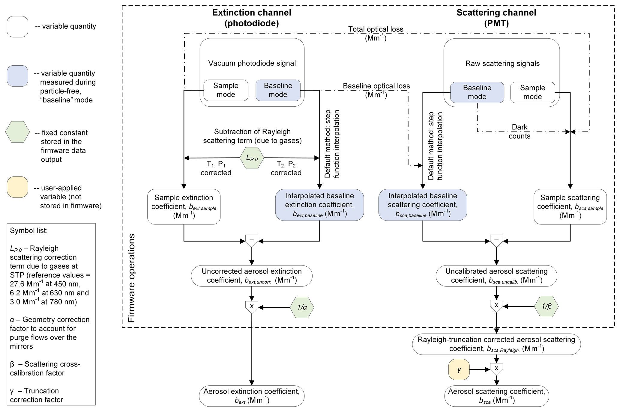
Figure 2Data processing chain for the extinction and scattering channels of the CAPS PMssa. Blue boxes indicate quantities that are measured during the periodic “baseline” mode of operation of the instrument. Hexagonal containers indicate fixed constants, and rounded rectangular containers represent variable quantities.
In the extinction channel, the sample and baseline measurements are first treated by subtracting out a constant factor that accounts for extinction due to Rayleigh light scattering from the aerosol carrier gas. The subtraction term is corrected using temperature and pressure measurements taken by the instrument to account for possible variations in these quantities between sample and baseline periods.
Full treatment of the PMT scattering signals is given by Onasch et al. (2015). The scattering signals are counted during the LED off-phase when only highly collimated light is circulating in the cavity in order to minimize the contribution of light scattered from interior surfaces of the instrument. Consequently, the average intensity of circulating light during the LED off-phase must be accounted for in the scattering calculation, as illustrated by the dot-dashed lines in Fig. 2 and described in detail in Onasch et al. (2015).
Following these initial data treatment steps, uncorrected aerosol extinction and uncalibrated scattering coefficients ( and , respectively) are obtained by taking the difference between the sample-mode coefficient measurements (which we term bext, sample and bsca, sample) and the interpolated baseline-mode coefficient measurements (bext, baseline and bsca, baseline). By default, the instrument firmware uses a step function to interpolate the baseline values between each baseline period (i.e., the mean value of a baseline period is assumed to stay constant until it is replaced by the mean value of the next baseline period). However, the data output files from the instrument also provide sufficient information for the user to apply custom methods for calculating the interpolated coefficients bext, baseline and bsca, baseline (e.g., linear or cubic spline interpolation; Pfeifer et al., 2020).
Following the sample-baseline difference calculations, one extinction correction factor (the geometry correction factor, α) and two scattering correction factors (cross-calibration, β, and truncation factors, γ) are multiplicatively applied to the respective signals in order to obtain the calibrated and corrected aerosol coefficients bext and bsca. The α and β factors are applied automatically by the instrument firmware, while γ must be applied manually by the user in post-processing. All three correction factors are discussed in detail in the sections below. The aerosol absorption coefficient is then obtained as
2.2.1 Geometry correction factor (α)
The purge flows that protect the high-reflectivity mirrors in the CAPS PMssa shorten the effective optical path length of the cavity and may slightly dilute the instrument sample flow at the cavity inlet. Therefore, a correction factor must be applied to the measured extinction coefficients in order to account for these changes (Massoli et al., 2010; Onasch et al., 2015; Petzold et al., 2013). We refer to this correction factor as the geometry correction factor, α, which can be determined by external calibration, i.e., by comparing CAPS PMssa measurements against independently measured or calculated bext (e.g., Mie-calculated bext values for spherical, monodisperse test aerosols, Petzold et al., 2013, or measured bext values for non-absorbing test aerosols obtained with a reference nephelometer, Pfeifer et al., 2020).
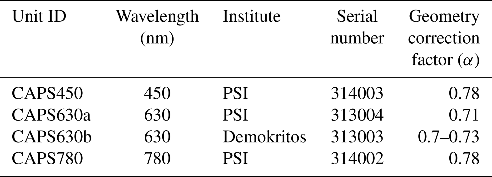
Onasch et al. (2015) applied the Mie calculation approach to measurements of polystyrene latex (PSL) spheres of varying diameter to determine an α value of 0.73 for a CAPS PMssa unit operating at 630 nm. This is lower than the general value of 0.79 quoted by Onasch et al. (2015) for CAPS PMex monitors, which they note is expected due to small differences in the cavity geometries. The CAPS PMssa units used in this study (Table 2) participated in European Center for Aerosol Calibration (ECAC; http://www.actris-ecac.eu/, last access: 29 January 2021) workshops (CAPS630b in August 2016 and CAPS450, CAPS630a, and CAPS780 in January 2017) where their geometry correction factors were determined against reference instrumentation (CAPS PMex, nephelometer) using ammonium sulfate test aerosols. The units were determined to have α values of 0.78 (CAPS450), 0.71 (CAPS630a), 0.7 to 0.73 (CAPS630b), and 0.78 (CAPS780). Therefore, it appears that α is instrument-unit-dependent. The stability of α over time is still an open question. However, regular and frequent measurements of α in CAPS PMex monitors performed at the ECAC suggests that it does not drift by more than 3 % over the period of a year. By default, the CAPS PMssa firmware automatically applies an α factor of 0.73 to calculate bext (Fig. 2).
Table 1Summary and description of uncertainties in the individual parameters comprising the error model described in Sect. 2.3. The precision column represents uncertainty due to the limited precision with which a particular parameter can be determined during calibration or measurement, and the drift column represents uncertainty due to possible drift of a parameter between available measurements. Estimated values are taken from previous studies or this study as indicated. The estimated values with units of Mm−1 correspond to absolute errors, and those with percentages relative errors.
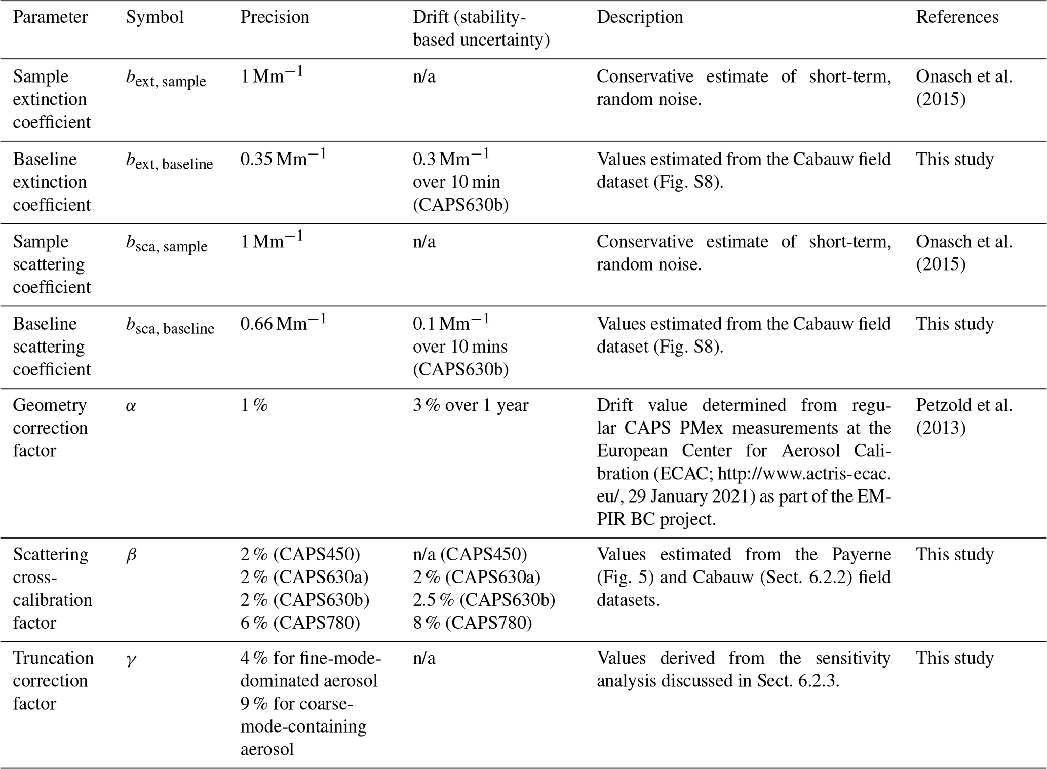
Table 2CAPS PMssa instrument units that were used in the present study.
2.2.2 Scattering cross-calibration factor (β)
The scattering cross-calibration factor (β) is used to relate the PMT-measured scattering signal of the CAPS PMssa to an absolute aerosol scattering coefficient. The value of β can be determined by cross-calibrating the uncalibrated aerosol scattering coefficient against bext measured by the extinction channel (Onasch et al., 2015). This approach is possible because the scattering and extinction coefficients are measured simultaneously for the same air sample, and bext measured using the CAPS method is effectively “calibration free” (apart from the geometry correction factor, as discussed in Sect. 2.2.1, as well as potential non-linearities at high baseline losses). Amongst other factors, β depends on the PMT detector response, which can vary over time. Therefore, regular cross-calibrations should be performed.
Non-absorbing test samples are required to perform the cross-calibration and to determine a value for β (i.e., purely scattering samples for which bext=bsca, or SSA = 1). In principle, the calibration can be performed with gases or aerosol particles. In practice, we performed all calibrations in the present study with particles because readily available calibration gases such as CO2 span a much smaller range in bsca than is achievable with aerosols of different concentrations, additional corrections are required to account for the changes in optical path length and dilution with the purge flows for different gases (see Sect. 2.2.1), and we have observed that the instrument can take a long time (∼ hours) to adjust and stabilize when filled with different gases (as expected due to the low flows and large filter areas in the purge flow setup).
When using the particle-based calibration method, non-absorbing aerosol particles with size parameters x in the Rayleigh light-scattering regime should be used to ensure well-defined scattered light truncation, since the scattering-phase function is independent of particle size in the Rayleigh regime. We term cross-calibration constants derived in this specific manner as βRayleigh. The size parameter x relates the aerosol particle diameter Dp to the wavelength of light λ through the expression πDp∕λ. The Rayleigh regime is defined by the condition x≪1. In practice, there is a trade-off between selecting particle sizes that are small enough to lie within or near the Rayleigh regime limit but large enough to generate scattering and extinction signals with sufficiently high signal-to-noise ratios. This means particles with diameter less than approximately 150 nm should be used to determine βRayleigh in the 450 nm CAPS PMssa, while slightly larger particles (e.g., Dp∼200 nm) can be used with 630 or 780 nm CAPS PMssa instruments.
Formally, the Rayleigh-regime, particle-based cross-calibration approach can be expressed as
where and are the extinction and uncalibrated scattering coefficients, respectively, for a population of non-absorbing particles with size parameters in the Rayleigh regime. The right-hand side of Eq. (3) is obtained by substitution of the relationship into the left-hand side ratio. From this substitution, it can be seen that βRayleigh (and β, generally) is directly proportional to the geometry correction factor α, which is required to measure bext accurately as discussed in Sect. 2.2.1 (the remaining fraction of the cross-calibration constant is termed to distinguish it from βRayleigh). Thus, Eq. (3) demonstrates how the cross-calibration approach quantitatively links bsca to bext in the CAPS PMssa. Following application of βRayleigh, we refer to the calibrated aerosol scattering coefficient corrected for the truncation of Rayleigh scattered light as bsca, Rayleigh. This is to recognize the fact that the cross-calibration approach represented by Eq. (3) implicitly corrects for the truncation of light scattered from the calibration aerosol, which has been chosen specifically to have the well-defined phase function corresponding to Rayleigh light scattering.
Onasch et al. (2015) demonstrated that the linearity shown by Eq. (3) is valid up to extinction coefficients of ∼1000 Mm−1, which is higher than typical ambient aerosol extinction coefficients, excluding perhaps coefficients in heavily polluted urban environments. The precise limit of linearity should be examined for individual instrument units if it is relevant for a particular experiment. For very high aerosol loadings above the limit of linearity the CAPS PMssa cross-calibration approach can still be used. However, this requires the addition of empirically derived higher-order terms in to Eq. (3). In addition, the potential occurrence of multiple scattering effects needs to be considered at very high aerosol loadings (Wind and Szymanski, 2002).
2.2.3 Truncation correction factor (γ)
The final quantitative correction factor that must be applied to the scattering coefficients measured with the CAPS PMssa is the truncation correction factor, γ. The truncation correction factor γ is applied to bsca, Rayleigh to compensate for the light scattered in near-forward and near-backward directions that is not measured by the instrument due to geometric restrictions. The truncation correction factor γ depends on both the instrument properties as well as the angular distribution of light scattered from the aerosol sample being measured (referred to in short as the ensemble scattering-phase function, Sp), which depends on the aerosol size distribution, morphology, mixing state, and composition (refractive indices). The existing methods for calculating the CAPS PMssa truncation correction factor γ either do not include the process of scattered light reflection from the inner surface of the glass sampling tube (Onasch et al., 2015) or are computationally expensive (Liu et al., 2018) and not well suited for calculating time-resolved truncation factors for large datasets (e.g., as required for the example Cabauw dataset in Sect. 6.2). Therefore, we present here a new truncation calculation framework that overcomes both of these limitations.
The new calculation framework is presented visually as a flowchart in Fig. 3. The full set of details and equations is given in Appendix A. Briefly, we define γ as the normalized ratio of the true integrated scattering coefficient, bsca, true, to the truncation-affected scattering coefficient that is actually accessible to measurement, bsca, meas. The true scattering coefficient bsca, true represents the coefficient that would be measured by an ideal integrating nephelometer capable of collecting light scattered in all possible directions. The ratio requires normalization by a factor kRayleigh to represent the fact that some scattered light truncation is already included implicitly in the cross-calibration constant, due to the way in which it is measured. For the recommended case of cross-calibration with Rayleigh scatterers according to Eq. (3), kRayleigh represents the truncation of the Rayleigh scattered light from the calibration aerosol. That is,
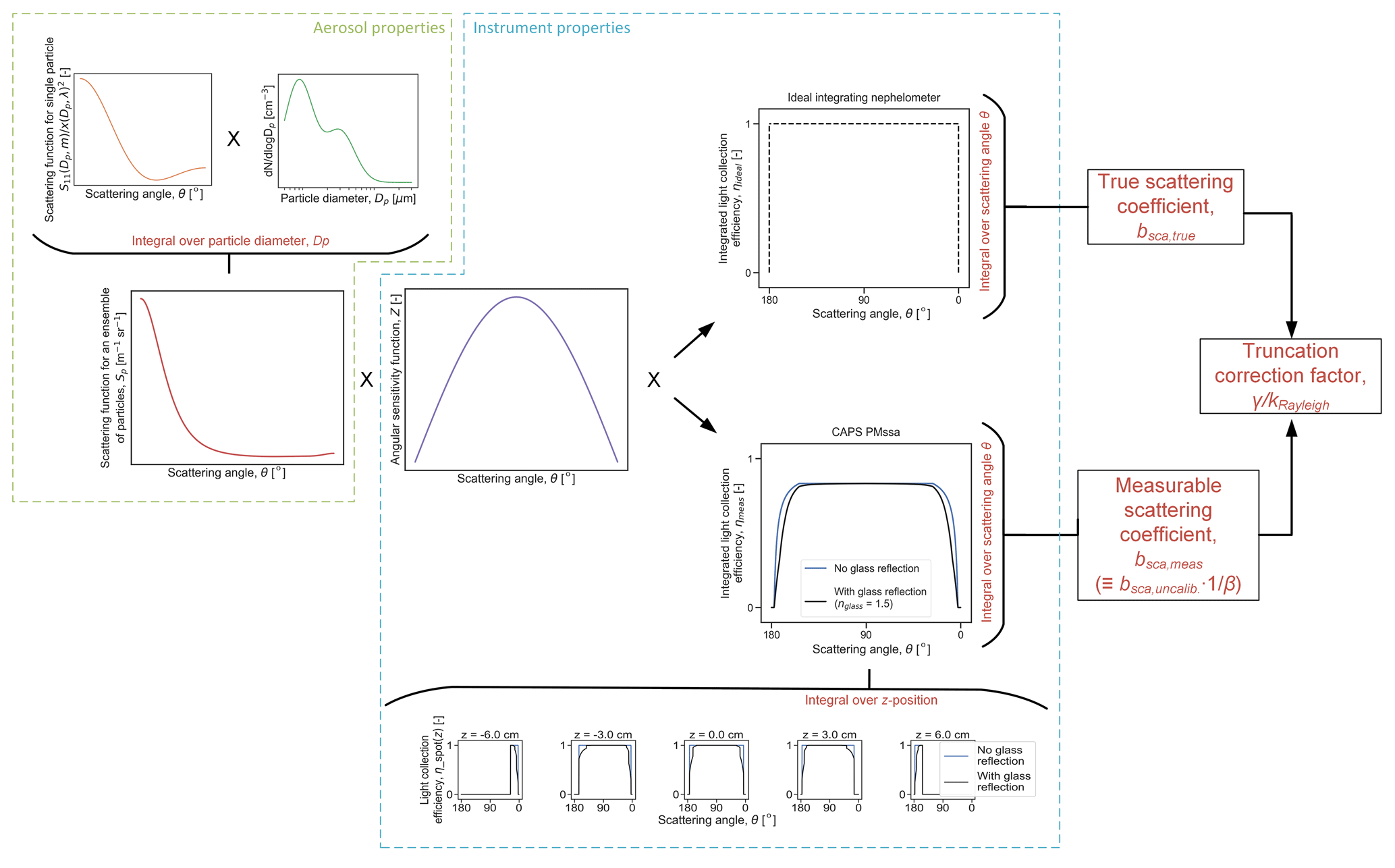
Figure 3Schematic diagram of the new model for calculating truncation correction factors for the CAPS PMssa. Full details of the calculations are presented in Appendix A. The model requires as input a light collection efficiency function and an angular sensitivity function, which are determined by the geometry of the CAPS PMssa optical system; and a scattered light intensity function for the ensemble of particles being measured, which is a function of the particle size distribution (dN,∕ dlogDp) and size-dependent aerosol scattering-phase function. The main output of the model is the truncation correction factor, γ.
Defined in this manner, γ equals 1 for aerosols in the Rayleigh regime. For aerosols containing larger particles or non-spherical particles that produce more forward-focused light scattering, γ is always greater than 1.
The equations for calculating the integrated scattering coefficients in Eq. (4) are detailed in Appendix A. These equations have been given in several previous publications (Anderson et al., 1996; Heintzenberg and Charlson, 1996; Moosmüller and Arnott, 2003; Müller et al., 2011b; Peñaloza, 1999). The novel aspect of our formulation is that we explicitly define a function representing the efficiency with which an integrating nephelometer is able to collect scattered light, η(θ, λ), which is a simple function varying between 0 and 1. Values of 0 indicate that a nephelometer collects no light of wavelength λ at some scattering angle θ, while values of 1 indicate that a nephelometer collects all the light scattered at angle θ. Considering η(θ, λ) explicitly has a number of advantages: (i) it allows transparent representation of an instrument's truncation angles (i.e., by setting η equal to 1 between two truncation angles and 0 beyond them), (ii) it allows for the simple and explicit introduction of additional physical processes into light-scattering calculations (e.g., reflection from the glass sampling tube can be considered by combining the Fresnel equation for reflection probability with η, as shown in Appendix A), (iii) it provides a clear and intuitive way to compare the abilities of different nephelometers to collect scattered light, and (iv) it emphasizes the modular nature of the truncation calculation.
One of the important characteristics of integrating sphere-type reciprocal nephelometers like the CAPS PMssa is that truncation is a function of position along the central axis of the optical cavity (which we denote as the z dimension, Fig. 1). This characteristic is represented by the small subplots in Fig. 3 that show light collection efficiency curves (termed ηspot in Appendix A) for six different z positions in the CAPS PMssa, including for two positions at 1 cm outside of the integrating sphere (i.e., and 6 cm). Positions outside of the integrating sphere must be considered since it is possible for particles outside the sphere to scatter light into the sphere (e.g., Varma et al., 2003), even if only through a narrow range of scattering angles. We term the extra length that needs to be considered outside the sphere's boundaries as the l parameter. The geometrical limits for the l parameter are 0 (i.e., no extra path length considered) and 4.7 cm (the distance between the integrating sphere and the sample inlet and outlet ports to the optical cavity). Onasch et al. (2015) and Liu et al. (2018) both used l=1 cm in their calculations (i.e., they considered a z range from −6 to 6 cm). The ηspot subplots in Fig. 3 also demonstrate the effect of glass tube reflection: between a sphere's truncation angles, reflection decreases the probability of light collection from 1 to some value less than 1. Therefore, glass tube inner surface reflection serves to increase scattered light truncation. A single, integrated light collection efficiency function for the CAPS PMssa can be generated by integrating ηspot over all possible z positions (Eq. A13). CAPS PMssa integrated η functions are shown in Fig. 3 for the two cases of without and with glass reflection.
It is important to stress the implications of the modularity of truncation calculation. This modularity means that once the η(θ, λ) and angular sensitivity functions are known for a particular instrument, they can be combined with any measured or calculated ensemble scattering-phase function in order to calculate γ. In the present study, we used Mie theory and co-located particle size distribution measurements to efficiently calculate hourly resolved Sp functions and γ values for a month-long field campaign (Sect. 6.2; Fig. S12). This Mie calculation method assumes spherical, homogeneous particles. If one wished to consider more complex particle morphologies, a more sophisticated optical model could be used to calculate the scattering-phase functions Sp, or if co-located polar nephelometer measurements of the scattering-phase function were available (e.g., Espinosa et al., 2018), these could be input directly into the truncation calculation.
2.3 Absorption error model for the CAPS PMssa and discussion of the sources and effects of uncertainties in β and γ
It is critical to carefully consider and understand the sources of errors in EMS-derived babs values, since these can be very large when taking the difference of two potentially larger numbers – bsca and bext – that each carry their own uncertainties. Based on the data processing framework presented in the previous Sect. 2.2, an error model can be constructed for CAPS PMssa absorption coefficients by considering the uncertainty in each of the individual parameters on the right-hand side of Eq. (2) and applying the standard rules of error propagation, including consideration of potential covariance of the errors in bsca and bext. The explicit equations for such a model are given in Appendix B. Table 1 lists the individual parameters in the error model along with realistic estimates of their uncertainties. In general, we consider two sources of uncertainties: uncertainty due to the limited precision with which a particular parameter can be determined during calibration or measurement and uncertainty due to possible drift of a parameter between available calibrations or measurements (e.g., baseline drift between two subsequent baseline measurements). For a given parameter, these two sources of errors are independent and can be added in quadrature, or if one of the errors is much larger than the other, this larger error can simply be used in error propagation calculations.
Many of the individual uncertainty estimates given in Table 1 are taken from previous studies and will not be discussed in great detail here. However, the uncertainties in the bsca correction factors γ and β are still poorly constrained and require further investigation. We refer to these uncertainties as δγ and δβ, respectively. Onasch et al. (2015) showed that β can be measured with high precision for a 630 nm PMssa unit, but the obtainable precision at other operation wavelengths as well as the stability in β over time have not been fully explored. Therefore, the overall δβ is still not well characterized.
The uncertainty in γ is more difficult to quantify. At the highest level it can be categorized into uncertainties related to the instrument properties (e.g., should glass tube reflection be considered, and an appropriate l value) and those related to knowledge of the scattering-phase functions of the aerosol samples being measured. Regarding uncertainties in the latter category, these can be further characterized depending on how the angularly resolved light-scattering information is obtained. In the best-case scenario, the scattering-phase functions would be obtained directly from co-located polar nephelometer measurements, in which case δγ would depend on the accuracy of these measurements (and possible extrapolation of those measurements beyond a polar nephelometer's truncation angles). Since polar nephelometer measurements are rarely performed in measurement campaigns, it is more likely that scattering-phase functions will be calculated with an optical model (e.g., Mie theory) using co-located size distribution measurements (covering both sub- and super-micrometer size fractions) as input. In this case, δγ will be a function of the accuracy of the input size distribution measurements, as well as the representativeness of the optical model and its inputs (e.g., complex refractive index, particle morphology if the optical model includes treatment of this). In the worst-case scenario, which is expected to occur frequently in field work, there might be no information available to constrain the scattering-phase function. In this case, γ values would need to be assumed. For example, a user might simply assume that γ equals 1, which is equivalent to assuming that all particles in the sample are Rayleigh light scatterers. In this case, δγ should reflect the possible consequences of that assumption. In Table 1 we provide some estimates for both δγand δβ that are based on the results of the present study. These estimates and results are discussed in specific detail below in Sects. 4, 5, and 6.
For now, we use our error model to assess the possible impacts of δγ and δβ on the relative uncertainty in EMS-derived babs, regardless of where the uncertainty in these two parameters actually comes from. Indeed, we generalize this analysis even further by considering the relative uncertainty in the combined bsca correction factor γ∕β, given by the equation
This approach is motivated by the fact that δγ and δβ have equal impacts on the uncertainty in EMS-derived babs, and it is justified because δγ and δβ are independent of one another.
The relative uncertainty in babs calculated with our error model can be interpreted as the precision with which babs can theoretically be determined for a given set of error model inputs. It should be noted that in addition to this precision-based uncertainty, the absolute accuracy of babs will also depend directly on the accuracy of the geometry correction factor α if the instrument is cross-calibrated as recommended in Sect. 2.2.2. This is because in the same manner as with bsca, the cross-calibration serves to define babs with respect to α, which can be seen by substituting the right-hand side of Eq. (3) into (2):
In the present study we do not explicitly consider the α-related uncertainty in babs, though it is important to keep this in mind. Specifically, we note that the errors in α cause covariant errors in bext and bsca. Hence, the relative error in α propagates 1-to-1 to the corresponding relative error in EMS-derived babs, independently of SSA. This is not the case for errors in , for example, which lead to an error in bsca that is independent of errors in bext and therefore relative errors in babs that do vary with SSA. In practice, the uncertainty due to α can only be determined by comparison of CAPS PMssa measurements against an independent reference. It is also worthwhile noting that the uncertainty in SSA measured by CAPS PMssa does not depend on the uncertainty in α, since this factor simply cancels out when taking the ratio of bsca to bext. This is one of the key design features of the cross-calibrated instrument (i.e., the relative error in α makes identical and covariant contributions to the errors in bext, bsca, and babs).
Focusing on the precision-related uncertainty in babs that is quantified by our error model (Eq. B2), Fig. 4 displays this variable as a function of the combined relative uncertainty in β and γ for a range of different atmospheric conditions (two different aerosol loadings and four different SSA values). The curves in this figure were generated using the following model inputs designed to represent the CAPS630b instrument characteristics during the Cabauw field campaign (Sect. 6.2): [α=0.73, δα=0, β=0.81, γ=1.04, Mm−1, Mm−1, Mm−1, Mm−1, and Mm−1]. Parameter δα was set to 0 to reflect the fact that the accuracy of α is not considered in the simulation as well as the assumption that α does not vary between subsequent cross-calibration measurements. Figure 4 can be interpreted as follows: taking an uncertainty of 5 % for γ and 2 % for β (which we will show later to be realistic estimates), the relative uncertainty in the combined bsca correction factor equals 5.4 % based on Eq. (6). This example corresponds to vertical blue dashed line in Fig. 4. Two other realistic examples are also shown in the figure as vertical dashed lines.
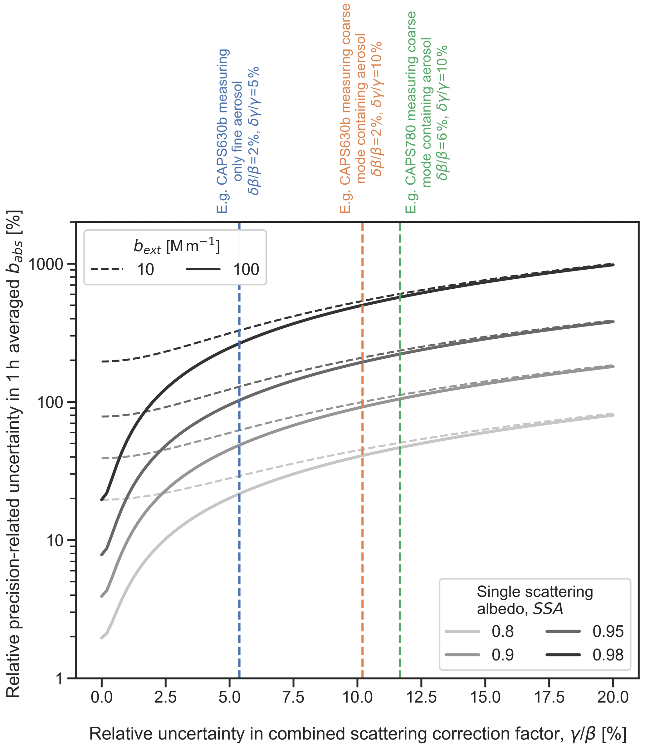
Figure 4Theoretically calculated relative uncertainty in 1 h averaged CAPS PMssa babs measurements as a function of the relative uncertainty in the combined scattering correction factor (defined in Eq. 5 using the ratio of the truncation correction factor γ and the instrument cross-calibration factor β). Curves are shown for four different SSA values (grey shading) and two different aerosol loadings (bext of 10 and 100 Mm−1). The curves were generated using the error model presented in Sect. 2.3 and Appendix B with inputs that were chosen to represent instrument characteristics during the Cabauw field campaign, as detailed in the main text.
Several important and general features are apparent in Fig. 4. Firstly, it is seen that the precision-related uncertainty in babs increases dramatically with small increases in uncertainty in either β or γ. As a result, small uncertainties in β or γ can result in large uncertainties in babs. The relative uncertainty in babs is also a strong function of SSA due to the large subtractive error amplification that results from taking the difference of two large and uncertain numbers. Taking these two points together and considering the example case demonstrated by the vertical red dashed line, a combined uncertainty of only 10.2 % in γ and β leads to precision-related uncertainties in babs of over 80 % at SSA greater than 0.9. Such large SSA is very common for atmospheric aerosols, which highlights why it is so critical to minimize uncertainties in β and γ when using the CAPS PMssa to measure atmospheric aerosol absorption with the EMS method.
The divergences between the corresponding dashed and solid grey lines in Fig. 4 represent the effects of the errors in both the extinction and scattering baseline signals. These errors can be important under very clean atmospheric conditions (represented by the case bext=10 Mm−1), since the absolute differences between sample-mode and baseline signals are then small. However, these sources of uncertainty are quickly overwhelmed as uncertainties in β and γ increase, resulting in the convergence of the pairs of dashed and solid grey lines moving from left to right across the figure. For the high aerosol load case (represented by bext=100 Mm−1), it is interesting to note that for 0 % uncertainty in β and γ, the relative uncertainty in babs is still SSA dependent, even though bsca has been defined with respect to bext by the cross-calibration and δα set to 0 in the simulation. This is because bext, sample and bsca, sample still carry independent uncertainty due to random noise, even if this is relatively small (i.e., 1 Mm−1 at 1 s temporal resolution).
The babs uncertainty values displayed in Fig. 4 were simulated to represent 1 h averaged measurements. Figure S1 indicates that the equivalent values representing 1 min averaged measurements are practically equivalent to those shown in Fig. 4, while those representing 1 s measurements are only greater for low values of uncertainty in β and γ. This is because of all the uncertainties listed in Table 1, only the uncertainties in bext, sample and bsca, sample are related to random noise and hence can be reduced by signal averaging. Since these error components are small relative to the other error components in the model, averaging for 1 min or 1 h has only a minor effect on the calculated uncertainty in babs.
3.1 Instrumentation
3.1.1 Instruments for measuring aerosol light absorption and black carbon concentrations
In this section we detail the experimental methods that we applied to investigate and characterize the ability of the CAPS PMssa to measure atmospheric aerosol absorption coefficients. A total of four different CAPS PMssa monitors were used in this study: one operating at 450 nm, two at 630 nm, and one at 780 nm. The four units are listed in Table 2 along with their relevant specifications.
A multi-angle absorption photometer (MAAP; Thermo Fisher Scientific, Waltham, MA, USA) was used during the Cabauw field campaign (Sect. 3.4.1) to measure absolute aerosol absorption coefficients at a wavelength of 637 nm (Petzold and Schönlinner, 2004). As discussed in the Introduction, the MAAP is a filter-based absorption photometer that incorporates additional measurements of back-scattered light and a two-stream radiative transfer scheme in order to constrain aerosol absorption coefficients more tightly than is possible with simple light attenuation measurements. The MAAP is a well-known and well-characterized instrument for measuring light absorption by atmospheric aerosols. The accuracy of MAAP absorption coefficients was investigated against laboratory reference EMS absorption measurements in the Reno Aerosol Optics Study (RAOS), and the two methods were found to agree within 7 % for a range of different black-carbon-containing aerosols (Petzold et al., 2005). Müller et al. (2011a) demonstrated that the unit-to-unit variability between six different MAAP instruments was less than 5 %. These authors also showed that the true operation wavelength of the instrument was 637 nm, not the nominal value of 670 nm. Assuming an absorption Ångström exponent of 1.02, a 5 % correction factor should be applied to the firmware output of the MAAP to account for this wavelength difference (Müller et al., 2011a). This correction factor was applied in the present study. A mass absorption cross-section value of 6.6 m2 g−1 was used to convert the equivalent BC mass concentrations reported in the firmware output of the MAAP to absorption coefficients (as specified by the manufacturer).
During the RAOS campaign (Petzold et al., 2005), MAAP absorption coefficients were observed to have no relationship with aerosol SSA. However, at extremely high SSA values the absorption coefficient measurements from the MAAP can be biased high. It is also important to consider that – to the best of our knowledge – no dedicated study has yet been performed to assess the precision and accuracy of MAAP measurements of samples containing a large fraction of super-micrometer particles. To quantitatively compare the MAAP and CAPS PMssa absorption coefficients during the Cabauw field campaign, both coefficients were adjusted to standard temperature (273.15 K) and pressure (1 atm). It should be stressed that in this comparison we do not consider the MAAP to be a true reference standard for measuring aerosol absorption coefficients. Rather, the value of the instrument for the present study lies in the fact that it displays very low instrument unit-to-unit variability, which means it can provide a common and stable reference point against which CAPS PMssa absorption measurements can be compared.
A single particle soot photometer (SP2; Droplet Measurement Technologies, Longmont, CO, USA) was used to measure black carbon mass concentrations at high time resolution from a mobile laboratory deployed during the Bologna field campaign (Sect. 3.4.2). The SP2 measures the mass of individual black carbon particles on a single-particle basis using the principle of laser-induced incandescence. The instrument has been described in detail previously (Schwarz et al., 2006; Stephens et al., 2003). Due to its very high sensitivity and responsiveness, its specific purpose in the present study was to provide a high time resolution reference time series of relative absorbing aerosol concentration. Its configuration during the present study is described by Pileci et al. (2020a).
3.1.2 Particle size classifiers applied for cross-calibration and truncation measurements
Two different types of aerosol size classifiers were used to generate monodisperse test aerosols for the purposes of measuring cross-calibration constants and scattered light truncation: an aerodynamic aerosol classifier (AAC; Cambustion Ltd, Cambridge, UK) and a differential mobility analyzer (DMA; custom-built version of the same design as the TSI Model 3081 long-column DMA, TSI Inc. Shoreview, MN, USA). The correct operation and sizing of both types of classifiers was confirmed throughout all the experiments by measuring nebulized PSL particles of different diameters (i.e., by operating the classifiers in scanning mode with downstream concentration measurements performed by a condensation particle counter).
The AAC classifies particles based on their relaxation time under the action of a centrifugal force generated in the annular gap between two rotating coaxial cylinders (Johnson et al., 2018; Tavakoli and Olfert, 2013). The particle relaxation time is related to the aerodynamic-equivalent diameter in a straightforward manner. In the context of highly size-dependent optical measurements, the major advantage of such a classification method is that it does not depend on particle electrical charge (unlike the DMA), which means the AAC can produce truly monodisperse distributions of particles (i.e., of finite width but without the presence of additional size distribution modes due to multiply charged particles). This charge-independent classification approach also enables higher aerosol transmission efficiencies than is possible with the DMA, which improves the signal-to-noise ratio of any downstream optical measurements. An additional advantage of the AAC relative to the DMA is that it can classify particles over a wider diameter range, including particles with diameters of up to ∼5 µm. The AAC was operated in the present study with the sheath-to-aerosol flow ratio of around 10:1, which results in geometric standard deviations for the classified aerosols of around 1.14. The set point aerodynamic diameters were converted to volume-equivalent diameters using literature values of particle density and assuming the classified particles were spherical.
3.1.3 Particle size distributions of ambient aerosol
Measurements of ambient particle size distributions were required during the Cabauw field campaign (Sect. 3.4.1) as inputs for the truncation correction calculations. These measurements were obtained by a scanning mobility particle sizer (modified version of the TSI SMPS 3034; TSI Inc. Shoreview, MN, USA) covering the mobility diameter range from 10 to 470 nm and an aerodynamic particle sizer (TSI APS 3321; TSI Inc.) nominally covering the aerodynamic diameter range from 0.54 to 20 µm.
The hourly averaged SMPS and APS size distributions were merged to create total aerosol size distributions covering the diameter range from 0.0104 to 10 µm for use in the truncation calculations. This was achieved by first converting the measured diameters of the respective instruments to volume-equivalent diameters. The SMPS electrical mobility diameters were simply taken to represent volume-equivalent diameter (i.e., shape effects were neglected). The APS aerodynamic diameters were divided by the square root of particle effective density to translate them into volume-equivalent diameters. A constant effective density of 2 g cm−3 was assumed. The joined size distributions were then created by linearly interpolating the SMPS and shifted APS measurements onto a common diameter scale between 0.0104 and 10 µm. The APS measurements of particles with physical diameters of less than 0.6 µm were not used in this joining calculation since they are known to display counting efficiency problems (Pfeifer et al., 2016).
3.2 Measurements of scattering cross-calibration constants
Scattering cross-calibration constants (Sect. 2.2.2) were measured with the experimental arrangement shown in Fig. S2. Ammonium sulfate particles or PSL spheres were generated in a Collison-type nebulizer and passed through a diffusion drier filled with silica gel for drying. A filtered bypass line was used after the nebulizer, and the ratios of the flows in this bypass line and the normal sampling line were adjusted to provide control on the concentration of the nebulized aerosol.
In the default laboratory setup, after drying the particles were passed through a size classifier to produce monodisperse distributions of particles with modal diameters less than 200 nm (i.e., to produce particles with size parameters less than approximately 1 that fall within or at least near the Rayleigh light-scattering regime; see Sect. 2.2.2). Additionally, to investigate a simplified procedure for potential application in field campaigns, selected calibrations were also performed by bypassing the size classifier. In this case only PSL particles with diameters less than 200 nm were produced with the nebulizer to keep the generated aerosol within or near the Rayleigh light-scattering regime. Nevertheless, it is possible that larger PSL aggregates (doublets or triplets) were also generated by the nebulizer. Such aggregates would be large enough to cause non-Rayleigh light scattering. In addition, large numbers of non-PSL, smaller particles (most with diameters <∼ 30 nm with tails extending to 100 nm or larger) are also produced when nebulizing PSL due to the presence of surfactants and other impurities in the PSL and Milli-Q water solutions. The composition of these particles is generally unknown. The possibility that they contained substantial absorbing components is unlikely but cannot be ruled out, which would violate the required cross-calibration condition that the calibration aerosol has SSA = 1.
In some of the calibrations a storage volume was placed upstream of the CAPS PMssa unit being calibrated. In these experiments the volume was first filled with calibration aerosol and the CAPS PMssa was then used to draw the concentration in the volume down to near zero. This enabled measurement of βRayleigh over a broad range of aerosol loads. In other cases the calibration aerosol was simply fed directly to the CAPS PMssa unit being calibrated. In all cases we limited the calibration measurements either during the experiment or later during data processing to bext values less than 1000 Mm−1 to avoid non-linearity issues between the scattering and extinction measurements (Sect. 2.2.2).
Two examples of scattering cross-calibration measurements are shown in Figs. S3 and S4. Figure S3 is an example of a calibration performed with 240 nm PSL particles with the storage volume present to enable measurement across a broad range of aerosol loadings, while Fig. S4 shows an example where the storage volume was not used such that the measurements only cover a narrow range of aerosol loading. The 240 nm PSL particles are slightly larger than the particles we typically use for cross-calibration, but these two examples are shown here to demonstrate the effect of the storage volume. The top panels of these figures show time series of the bext and , and the bottom left panel displays these variables in a scatterplot on a log–log axis. Onasch et al. (2015) determined βRayleigh as the gradient of a line fit to the scatterplot data. To avoid any potential linear fitting artifacts caused by outlying measurements, we elected to determine βRayleigh as the mean value of the ratio of for bext values greater than 50 Mm−1. This lower limit was chosen to avoid low signal-to-noise ratio measurements affecting the determined βRayleigh. The bottom right panels of Figs. S3 and S4 display histograms of the ratio (with the condition bext>50 Mm−1). It is seen that the values of the ratio are typically normally distributed, regardless of whether the measurements covered a broad range of extinction values or not (Fig. S3 vs. S4). We take the standard deviation of the measured ratios to represent the precision with which βRayleigh can be determined.
3.3 Measurements of scattered light truncation as a function of particle diameter
The general experimental setup that is shown in Fig. S2 was also used to measure scattered light truncation as a function of particle diameter, in order to validate our new truncation calculations (Sect. 2.2.3). Size-resolved truncation measurements can be performed directly with the CAPS PMssa using size-classified, non-absorbing test aerosols and taking bext as bsca, true and bsca, Rayleigh as bsca, meas in Eq. (4). Similarly to the cross-calibration constant βRayleigh, we applied a threshold condition of bext>50 Mm−1 when calculating mean ratios of bext to bsca, Rayleigh. For this application, the AAC was always used as the size classifier, since the AAC is able to generate truly monodisperse distributions of particles (i.e., finite width but without additional size modes due to multiply charged particles) and provides a larger upper size limit.
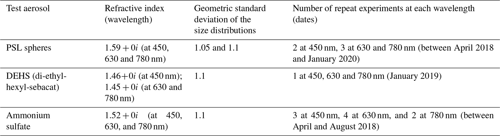
We measured truncation values for three different types of non-absorbing aerosols: PSL, DEHS (di-ethyl-hexyl-sebacat), and ammonium sulfate. The relevant properties of these aerosols are listed in Table 3. Three aerosol types were used in order to check consistency across different aerosols to provide more robust results. Nebulized and dried PSL and DEHS particles are spherical, while dried ammonium sulfate particles are at least near-spherical (e.g., Biskos et al., 2006). Spherical or near-spherical particles were used so that the aerosol-phase functions could be calculated precisely with Mie theory. The geometric standard deviations of the monodisperse DEHS and ammonium sulfate aerosols were nominally around 1.14 as determined by the operating conditions of the AAC (Sect. 3.1.2). We used geometric standard deviations of 1.1 in our model calculations for these two aerosol types. The widths of PSL size distributions are size-dependent and generally narrower than the transfer function of the AAC as used in these experiments. Therefore, we considered two geometric standard deviations of 1.05 and 1.1 in our model calculations for PSL. Rayleigh normalization factors (i.e., ; see Eq. 4) were measured at the beginning of each experimental run using particles of the given aerosol type with size parameters less than or close to 1. A number of repeat experiments were performed for some of the aerosol types, as indicated in Table 3.
Table 3Test aerosols used to measure scattered light truncation in the CAPS PMssa as a function of particle diameter and the values of parameters used in the corresponding model calculations. All particles were size classified by AAC.
3.4 Field measurements
3.4.1 Cabauw campaign
The Cabauw field campaign was conducted from 11 September to 20 October 2016 at the KNMI (Koninklijk Nederlands Meteorologisch Instituut) Cabauw Experimental Site for Atmospheric Research (the Netherlands; 51∘58′ N, 4∘55′ E; −0.7 m a.s.l.). The campaign was conducted in the framework of the ACTRIS project (WP11) and occurred simultaneously with the CINDI-2 MAX-DOAS intercomparison campaign (Kreher et al., 2020). The CAPS630b unit was the CAPS PMssa instrument deployed during this campaign to measure absorption coefficients at 630 nm. Absorption coefficients were also measured at 637 nm with a MAAP (Sect. 3.1.1). Particle size distributions were measured with an SMPS and APS (Sect. 3.1.3). All instruments were housed in a laboratory at the base of the KNMI-mast Cabauw behind identical inlets consisting of PM10 sampling hats protruding 4.5 m from the laboratory roof. The inlets contained large diameter Nafion driers, which kept relative humidity in the sampling lines below 50 %. All the data used in the present study were averaged over 1 h periods. This includes the joined SMPS and APS size distributions (Sect. 3.1.3), which used to calculate hourly resolved truncation correction factors using the model presented in Appendix A.
3.4.2 Bologna campaign
The Bologna field campaign was conducted from 5 to 31 July 2017. This campaign was also conducted within the framework of the ACTRIS project. The full campaign consisted of multiple stationary measurement sites that were centered around the city of Bologna in Italy's Po Valley. Additionally, a heavily instrumented mobile measurement van (the MOSQUITA; Bukowiecki et al., 2002; Weimer et al., 2009) travelled between the stationary sites to perform spatially resolved measurements of black carbon concentrations and properties. The results of these mobile measurements are presented by Pileci et al. (2020a). In the present study we use only 1 h of mobile measurements that were performed from the MOSQUITA while it was travelling on the heavily trafficked A1 highway between Bologna and Lodi on the morning of 25 July 2017. During this time period absorption coefficients were being measured with the CAPS780 and black carbon concentrations with an SP2 (Sect. 3.1.1).
3.4.3 Payerne campaign
The Payerne field campaign was conducted from 26 August 2019 to 14 January 2020 in Payerne, Switzerland, and involved the PMssa units CAPS450 and CAPS780. The goal of this campaign was to compare the hygroscopic properties of aerosols measured using remote sensing and in situ techniques. In the present study we only present the results of the CAPS PMssa cross-calibrations that were performed for the campaign: no ambient measurements are shown. In addition to the cross-calibrations that were performed at the Payerne field site with the CAPS450 and CAPS780 units, we also present the results of calibrations performed immediately before and after the campaign in the Aerosol Physics Laboratory of the Paul Scherrer Institute. In addition to the other two PMssa units, the CAPS630a was also included in these laboratory calibrations.
The cross-calibration constants that were measured for the CAPS450, CAPS630a, and CAPS780 PMssa units during and around the Payerne field campaign are presented in Fig. 5. These measurements are used to assess the stability of the cross-calibration constant (variability over the time series) and the precision with which it can be determined (error bars represent the ±1 standard deviation of the ratios of to bext for each calibration, as visualized in the lower right panels of Figs. S3 and S4). Some of the measurements were performed on size-classified aerosols (solid plot markers), and some were performed without classification (open plot markers), as discussed in Sect. 3.2.
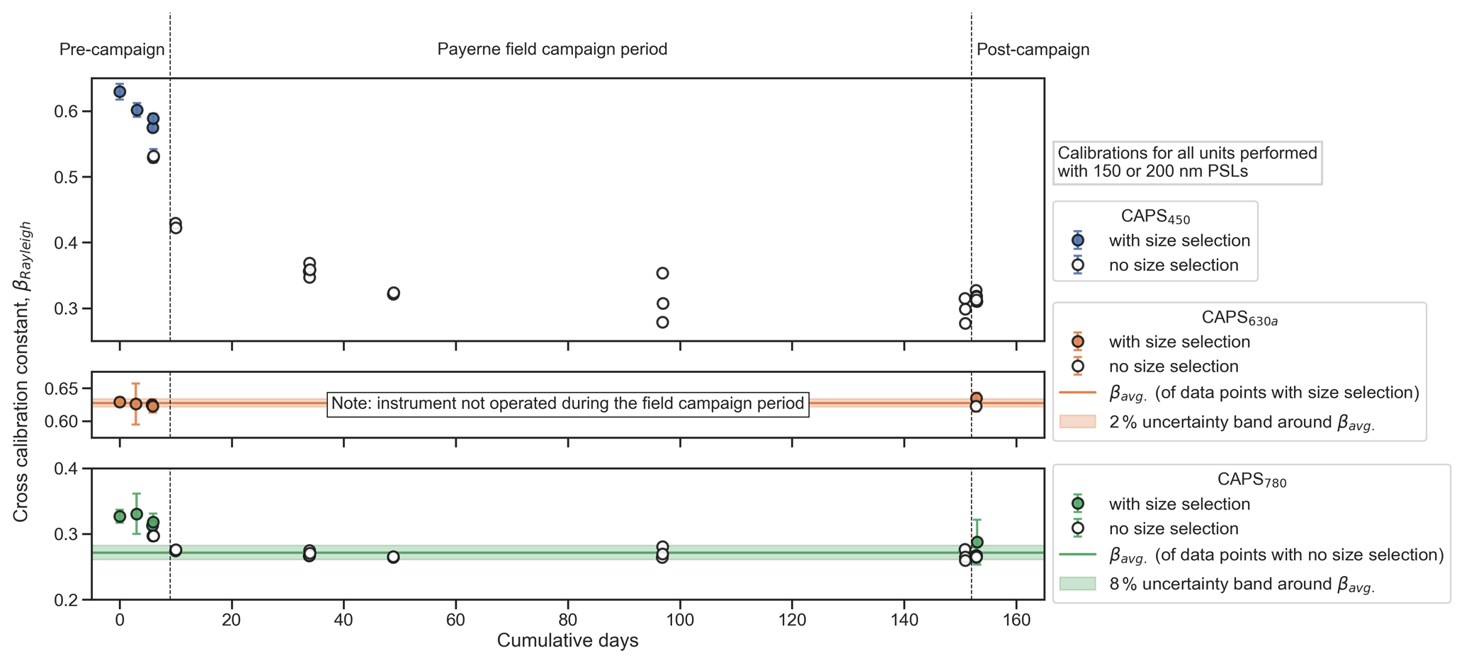
Figure 5Rayleigh-regime cross-calibration constants (βRayleigh) for three CAPS PMssa units (CAPS450, CAPS630a, CAPS780) measured before, during, and after the Payerne field campaign. Error bars indicate the standard deviation of the measured ratios used to determine each βRayleigh value (see Sect. 3.2).
To investigate the effect of size classifying the aerosol, four calibrations were purposely performed back-to-back, with and without an AAC size classifier. The results of these back-to-back calibrations are plotted on their own in Fig. S5. In two cases, the cross-calibration constants determined with and without size classification were similar (CAPS630a with a difference of −1.9 % between calibrations and CAPS450 run2 with a difference of 2.8 %). However, in the other two cases the βRayleigh value determined without size classification was substantially less than the value determined with classification: −9.7 % difference for CAPS450 run1 and −6.6 % difference for CAPS780. This is likely because of the presence of PSL doublets or triplets or because the non-PSL particles that are unavoidably generated during the PSL nebulization process either contained absorbing components or were big and abundant enough to cause substantial non-Rayleigh light scattering. In any case, we assume that the cross-calibrations performed with size classification provide the most trustworthy measurement, since it is more certain that all the required conditions for the cross-calibration are met.
Despite the potential differences between size-classified and non-size-classified measurements, some important results are still clearly seen in Fig. 5. Firstly, it is apparent that the variability in βRayleigh over time is instrument-dependent. The different behaviors observed for these three PMssa units represent the range of performances we have observed for CAPS PMssa monitors in the field. The least stable unit in this context was the CAPS450. In the 10 days prior to the beginning of the campaign, βRayleigh for CAPS450 was observed to decrease from 0.63 to 0.53. During the campaign itself, βRayleigh ranged from 0.43 to 0.28, showing a general decreasing trend as the campaign progressed. This observed drift corresponds to tens to hundreds of % of uncertainty in babs (Fig. 4). The CAPS450 instrument diagnostics provided no evidence of instrument malfunction, change, or contamination during this period. Therefore, this example demonstrates that regular cross-calibration validation measurements are necessary to exclude significant drifts. Given that the precise reason for instability in βRayleigh is unknown, we refrain from providing a stability-based uncertainty estimate for this unit in Table 1. However, the four individual AAC-based calibrations performed in the laboratory prior to the beginning of the campaign still provided a chance to investigate the precision-based uncertainty in βRayleigh for CAPS450. The average standard deviation of the ratios of to bext measured during these four calibrations was 0.009, which is 1.5 % of the average βRayleigh of 0.60. Therefore, we conservatively estimate that the βRayleigh can be determined with a precision of 2 % for this unit (Table 1).
The averaged value of βRayleigh for CAPS780 was 0.27 over the 14 measurements taken during the 140 d of the campaign (from days 10 to 151 on the cumulative days' x axis). The minimum and maximum values measured during this period were 0.26 and 0.28, respectively. Thus, we conservatively estimate a stability-derived uncertainty value of 8 % (δβRayleigh∕βRayleigh) for this unit in Table 1 while noting that this estimate is derived from calibration measurements without a size classifier, which may have contributed to the observed variability. The 8 % uncertainty range is represented by the green-shaded uncertainty band in Fig. 5. The precision-based uncertainty estimate in βRayleigh for this unit is determined from the five AAC-based cross-calibrations performed in the laboratory before and after the campaign (i.e., the average size of the green error bars). From these measurements we calculate a precision-derived uncertainty of 6 %. The CAPS630a was not operated during the Payerne field campaign period. However, laboratory measurements before and after the campaign indicated that βRayleigh for this unit can be determined with a very high precision of 2 % and is stable to within 2 % over time. We believe that this unit represents an example of the best-case performance for cross-calibration precision and stability that is possible with the CAPS PMssa.
In addition to continual drifts in βRayleigh over time, it is also interesting to note how βRayleigh can change following known instrument-malfunction events such as contamination of the PMssa optical cavity. Figure S6 displays CAPS PMssa measured bext (left panel) and bsca (right panel) at 450 nm against independent measurements of these quantities (CAPS PMex for bext, nephelometer for bsca) during a field campaign at the rural background site of Melpitz, Germany. For the duration of these measurements the optical cavity of the 450 nm PMssa unit became contaminated, moving the instrument outside of its intended range of operation, with average baseline optical loss varying from 758 to 1248 Mm−1. Such contamination events can occur due to large pressure fluctuations in the aerosol sampling line or failure of the instrument's purge flow system. They do not occur just by measuring high aerosol loads. In this case, the instrument-malfunction contamination event caused an increase in the bias of the bext measurement relative to the corresponding PMex measurement from 5 % to 17 %. However, over the same period, the bias of the bsca measurement with respect to the corresponding nephelometer measurement was unchanged, which implies that βRayleigh did change. Therefore, as specified by the manufacturer, we recommend that the CAPS PMssa baseline should be monitored continuously throughout measurement campaigns for signs of mirror contamination and that contaminated mirrors are cleaned promptly.
The results of the laboratory truncation measurements as a function of AAC-selected particle diameter are shown in Fig. 6 for both PSL and DEHS test aerosols. We refer to these curves as “truncation curves”. Truncation curves are a useful way to validate truncation calculations since the particle size is a key determinant of the aerosol scattering-phase function and consequently γ for spherical particles of known constituent material. Following earlier studies (Liu et al., 2018; Onasch et al., 2015), we display measured truncation values as the inverse of γ as defined by Eq. (4). Measurements are presented at three different wavelengths (corresponding to the three figure columns) as measured by the CAPS450, CAPS630a, and CAPS780 PMssa units. The equivalent measurements for ammonium sulfate are shown in Fig. S7. These results are not included in Fig. 6 since we suspect that the ammonium sulfate particles were slightly non-spherical after nebulization and drying, which makes them less useful for comparison with Mie-theory-based model curves, as is done below. Nevertheless, it is seen that the ammonium sulfate measurements are qualitatively consistent with the PSL and DEHS results over many repeated experiments. The PSL measurements at 450 and 630 nm presented by Onasch et al. (2015) are also included in Fig. 6. They indicate less truncation than the corresponding measurements from the present study. The reasons for these discrepancies are not entirely clear but may be related to the fact that the Onasch et al. (2015) measurements were obtained after size classification by DMA, although the authors found no substantial evidence of additional size distribution peaks due to multiply charged particles (and such particles would anyway cause greater truncation, not less).
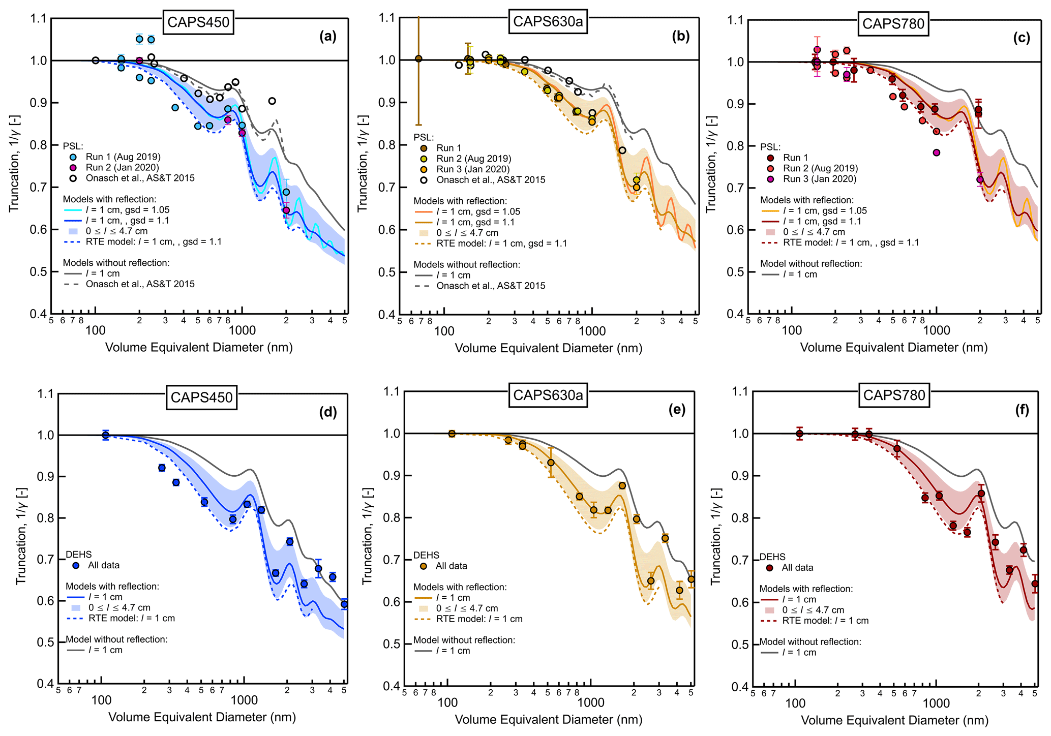
Figure 6Measured and modeled truncation values as a function of volume-equivalent particle diameter for PSL and DEHS aerosols. The truncation values plotted on the y axes correspond to the inverse of the truncation correction factor γ defined by Eq. (4). Modeled curves were calculated with the truncation model presented in Appendix A as well as the radiative transfer equation (RTE) model presented by Liu et al. (2018). The parameter l represents the extra path length beyond the integrating sphere, and gsd refers to the geometric standard deviation of the modeled test aerosols.
A variety of modeled truncation curves are also displayed in each panel of Fig. 6 for comparison with the measurements. Broadly, these can be classified into calculations that include the process of scattered light reflection from the inner surface of the glass sampling tube and those that do not. One uncertain parameter is the extra path length outside the integrating sphere that contributes to scattered light collection (the l parameter), which was set to 1 cm in the original model calculations by Onasch et al. (2015) without considering glass tube reflection (dashed grey lines in panels a and b). The corresponding truncation curves calculated with the new model presented in Appendix A and with the process of glass tube reflection switched off (solid light grey lines) agree well with the original model. Calculations made with the new model with the process of glass tube reflection turned on and l set to 1 cm are shown as the solid colored lines. The shaded envelopes around these curves demonstrate the sensitivity of modeled truncation to variation of l between its lower and upper geometrical boundaries (0 cm cm). Finally, the dashed colored curves in each panel are truncation curves calculated with the RTE-based model presented by Liu et al. (2018). These curves include the process of glass tube reflection and assume l=1 cm.
Measured and modeled truncation curves all display the same general features. Truncation values are relatively flat up to a volume-equivalent diameter of around 200 nm (or ∼150 nm at the 450 nm wavelength). This corresponds to the approximate limit of the Rayleigh light-scattering regime. At larger diameters, particles begin scattering relatively more light in near-forward directions, where it escapes from the CAPS PMssa integrating sphere. As a result of this loss of scattered light, the truncation curve begins decreasing with increasing particle diameters in a complicated but well-known manner due to the variation of the scattering-phase function with particle diameter. Specifically, at diameters >∼1 µm, peaks in the truncation curves occur due to Mie resonances. The peaks are slightly broadened by the small polydispersity of the AAC-selected size distributions. This can be seen when comparing the Onasch et al. (2015) modeled curves, which were calculated assuming a perfectly monodisperse distribution of particles, and the modeled curves from the present study, which consider the finite width of the experimental size distributions (in the case of PSL two geometric standard deviations of 1.05 and 1.1 are modeled). The remarkable fact that the Mie resonances are discernible in the measured PSL and DEHS truncation curves, even if perfect quantitative agreement is not obtained with the models, provides high confidence in the AAC-CAPS PMssa setup for measuring scattered light truncation. The Mie resonances are not as apparent in the ammonium sulfate measurements, which we suspect is likely due to particle non-sphericity as mentioned above.
In general, good agreement is obtained between the new model calculations including the process of glass tube reflection and the RTE model calculations. This is encouraging given these models are based on fundamentally different approaches for calculating truncation. Both of these modeled curves predict generally greater truncation than the calculations that neglect the process of glass tube reflection, as expected from theoretical considerations (Sect. 2.2.3). The measurements are in better agreement with the modeled curves that include glass tube reflection, demonstrating that this process must be considered in the calculations. This is a robust result that is consistent across all three aerosol types for particle diameters up to 5 µm and all three optical wavelengths that were investigated.
Considering the calculations made with the new model presented in Appendix A, the best agreement with the measured data appears to be obtained for an l value of 1 cm. However, there is enough scatter in the measurements to argue that any l value is plausible within the geometric limits of this parameter (from 0 to 4.7 cm). Although varying l over this range captures the measurements well, we stress that this does not imply that variable l is the physical reason for the measurement imprecision. For one, it can be argued that the lower limit l value of 0 cm is unrealistic since it is expected that particles at the boundary of the sphere will certainly scatter light into the sphere. Similarly, our model uses an idealized geometry of the interior of the CAPS PMssa cell. Nevertheless, varying l from 0 to 4.7 cm produces differences in calculated truncation that are similar to the differences observed between repeat measurements, as well as to the differences between calculations made with the two models that include the process of glass tube reflection (i.e., the model presented in Appendix A and the RTE model). Therefore, similarly to Onasch et al. (2015), we use l as a convenient tuning parameter to produce an uncertainty envelope that captures the range of measured truncation curves reasonably well.
6.1 Bologna example: instrument sensitivity and rapid response time
Two key features of the CAPS PMssa as a flow-through, continuously measuring optical instrument are its sensitivity and rapid response time. Onasch et al. (2015) demonstrate the instrument is able to respond to changes in bext and bsca of less than 1 Mm−1 on timescales of only ∼1 s. These specifications suggest that EMS-derived babs values measured by CAPS PMssa will display similar responsiveness and sensitivity. If so, these specifications would represent a major improvement over the equivalent specifications for babs values measured by filter-based absorption photometers, which are based on the slower process of accumulation and detection of aerosol samples on a filter.
To investigate these features under real-world conditions, Fig. 7 presents co-located measurements of aerosol absorption coefficients obtained with the CAPS780 instrument and rBC mass concentration measurements obtained with an SP2. The measurements were obtained while travelling along a busy highway road in a mobile laboratory near Bologna, Italy, where black carbon was shown to be the dominant source of absorbing aerosol. Indeed, the observed correlation between the independent measurements of black carbon and aerosol absorption is remarkably good, especially given the short averaging time of 5 s. In particular, the sharp peaks that are observed in both time series are found to align with each other extremely well. These peaks correspond to black carbon emissions from passing vehicles on the highway. Although this is only a 1 h sample of data, this example demonstrates the EMS-derived babs values can be measured at very high time resolution with the CAPS PMssa, comparable to what can be achieved with the single-particle level measurements of rBC mass from an SP2.
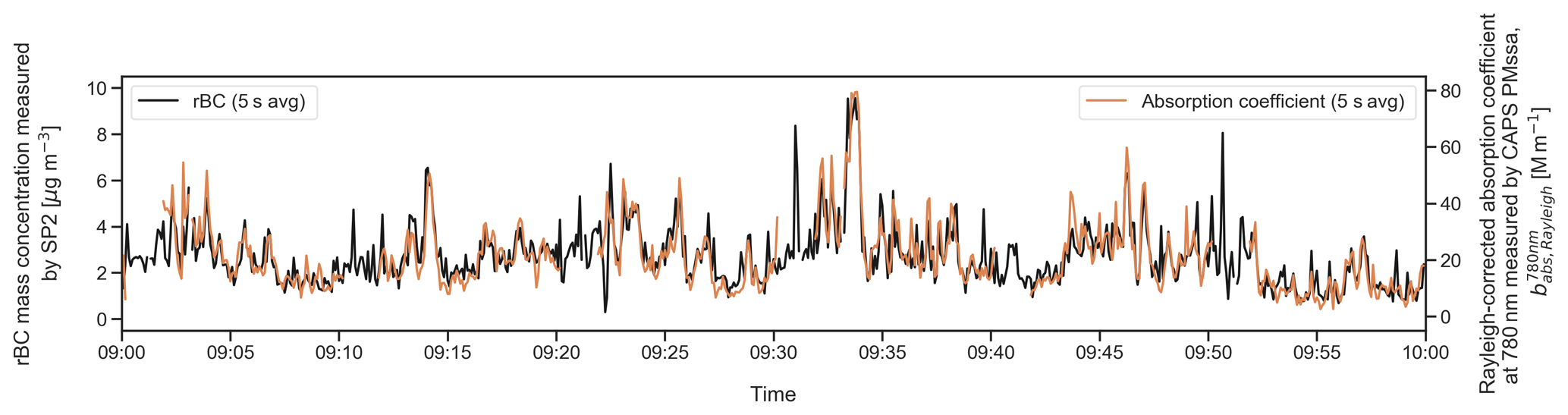
Figure 7Time series of a 1 h period of 5 s averaged rBC mass concentration and absorption coefficient measurements made from the mobile laboratory traveling on a highway road during the Bologna campaign. rBC mass concentrations were measured by SP2 – a sensitive, single-particle-based instrument. Absorption coefficients were measured at 780 nm with the unit CAPS780. Note that the absorption coefficients have only been corrected for Rayleigh scattering truncation and therefore should not be interpreted quantitatively (e.g., they cannot be used to calculate mass-absorption cross sections for the BC). In addition, the SP2 measurements have not been corrected for missing mass and should also not be interpreted quantitatively (Pileci et al., 2020b). Spikes in the time series correspond to emissions from passing vehicles on the highway.
Although Fig. 7 demonstrates the responsiveness of the CAPS PMssa, it must be stressed that the absolute values of the plotted babs measurements are still uncertain and should not be used quantitatively (the SP2 measurements of rBC mass are also underestimated and should not be used quantitatively, since the instrument was unable to detect an unknown fraction of the total rBC mass due to the small size of the freshly emitted BC cores; Pileci et al., 2020b). Specifically for the CAPS PMssa measurements, the plotted quantity is babs, Rayleigh to indicate that the underlying bsca measurements have not been corrected for the truncation of non-Rayleigh scattered light. To do so accurately would require co-located, equally high time resolution measurements of either scattering-phase functions or information that could be used to calculate phase functions (e.g., size distributions, fractal BC properties) for the freshly emitted BC-containing emissions plumes. Nevertheless, the ability to measure relative babs values at high time resolution with the CAPS PMssa creates possibilities for new types of experiments that were not previously feasible with traditional absorption photometers.
6.2 Cabauw example: comparison of CAPS PMssa absorption measurements against independent measurements with a MAAP
In this section we use an example dataset from the Cabauw campaign to make a direct absorption instrument-to-instrument comparison between the CAPS PMssa and the MAAP. This comparison is performed in order to gain insight into the ability of the CAPS PMssa to measure absolute aerosol absorption coefficients. As discussed in Sect. 3.1.1, the MAAP was used for this comparison because it provides stable and reproducible absorption measurements. However, it should be reiterated that the MAAP is not a true absorption reference standard: this instrument is associated with its own measurement uncertainties, which are not well characterized for aerosols with large contributions of super-micrometer particles. Despite these issues, our focus here is only on the uncertainties related to the CAPS PMssa absorption measurements, including detailed characterization of the scattered light truncation effect. The CAPS630b was the PMssa unit operated during the Cabauw campaign. The unit ran autonomously, continuously, and stably over the 1 month of operation, which we have found to be typical for CAPS PMssa units operated at stationary field sites.
6.2.1 CAPS PMssa baseline characteristics
The scattering and extinction baseline measurements over the campaign are displayed in Fig. S8. These measurements were performed for 1 min every 10 min using the auto-baselining feature of the instrument. The average standard deviations of the extinction and scattering baseline measurements over all 1 min baseline periods were 0.35 and 0.66 Mm−1, respectively. We take these values to represent the precision-based uncertainty estimates in bext, baseline and bsca, baseline in Table 1. Both baseline time series indicate that the optical cavity was generally clean and suffered no major contamination events during the campaign. Figure S8 also contains time series of the baseline drift in each channel, which were calculated from the differences between two successive baseline measurements (i.e., over a period of 10 min, which means the calculated metric does not include possible variations over shorter timescales). On average, the extinction baseline drifted by 0.026 Mm−1 min−1 and the scattering baseline by 0.013 Mm−1 min−1. Individual values of up to 0.3 and 0.09 Mm−1 min−1 were observed in the extinction and scattering channels, respectively. To minimize the impacts of these drifts, both the extinction and scattering measurements were reprocessed using the method of linear interpolation between successive baseline measurements (Pfeifer et al., 2020). Figure S9 indicates that this reprocessing had a noticeable effect at a 1 s time resolution for bext values less than ∼20 Mm−1 and bsca values less than ∼5 Mm−1. However, these effects are averaged out when considering hourly averaged data.
6.2.2 Uncertainties in the CAPS PMssa bsca correction factors β and γ
The cross-calibration constant for the CAPS630b could be measured with high precision (∼2 %) and appeared to be very stable based on measurements at the beginning (0.82; Fig. S10) and at the end of the campaign (0.80; Fig. S11), which differed by only 2.5 %. This is comparable with the optimum performance we have observed for CAPS PMssa units with regards to cross-calibration (see Sect. 4).
In the absence of direct scattering-phase function measurements, hourly time-resolved truncation correction factors were calculated with the Mie-theory-based model presented in Appendix A. Joined size distributions measured by SMPS and APS were input into the model. To estimate the uncertainty in γ a sensitivity analysis was performed with respect to the model's input parameters. This analysis is presented in the Supplement as Sect. S1 and visualized in Fig. S12. Specifically, we investigated the sensitivity of γ to the ambient aerosol refractive index (real parts between 1.50 and 1.59 and imaginary parts between 0.00 and 0.01, based on the summary of measurements presented by Espinosa et al. (2019), the l parameter (varied from 0 to 4.7 cm based on the results presented in Sect. 5), and the accuracy of the coarse-mode size distribution measurements between diameters of 2.5 and 10 µm. The truncation correction was found to be most sensitive to the l parameter (∼4 % across the range of tested parameters), weakly sensitive to the real part of the refractive index and size distribution information between 2.5 and 10 µm, and barely sensitive at all to complex part of the refractive index (not shown). Overall, we estimate an uncertainty in γ of 6 % for the Cabauw campaign based on this analysis (difference between the minimum and maximum average values of all the simulated distributions shown in Fig. S12). However, it must be stressed that this estimate is limited by our Mie-theory-based calculations, which do not include potential effects due to morphologically complex particles such as freshly emitted fractal BC aggregates. That is, the estimate only covers the parametric uncertainty in our Mie-theory-based calculations.
6.2.3 Truncation effects for fine-mode-dominated and coarse-mode-containing samples
The distributions of the time-resolved truncation correction factors calculated over the Cabauw campaign are clearly bi-modal (Fig. S12). This indicates that there were two limiting types of aerosols measured during the campaign: (i) fine-mode-dominated aerosol that only required a minor truncation correction; and (ii) aerosol with a substantial coarse-mode fraction that required a larger truncation correction. For further investigation, we extracted two subsets of data representing the fine-mode-dominated and coarse-mode-containing samples. This was done by selecting those aerosols whose coarse-mode number fractions (defined as calculated from size distributions) are in the lower and upper quartiles of all the data, respectively. The median normalized size distributions for these two categories are plotted in Fig. S13. The figure clearly shows a coarse mode of particles with diameters between ∼0.6 and 5 µm that was present in the coarse-mode-containing samples but not the fine-mode-dominated aerosols. Despite the small number fractions, these coarse-mode particles can make substantial contributions to the scattering coefficients, and they produce a greater fraction of forward- and backward-scattered light, thereby affecting truncation disproportionately.
The distributions of the time-resolved γ values for the fine-mode-dominated and coarse-mode-containing groups of samples are displayed in Fig. S14 (for the same ranges of model inputs that were examined for the full Cabauw dataset in Fig. S12). As expected, the required truncation correction values are substantially smaller for the fine-mode-dominated group than the coarse-mode-containing samples. This follows from the normalized ensemble scattering-phase functions for each group, which are displayed in the right panel of Fig. S13. These functions were calculated from the median size distributions with Mie theory and an assumed refractive index of 1.59+0.01i (functions like these are required as inputs for the γ calculation, as shown in Fig. 3). It is seen that the phase function for the fine-mode-dominated category is less focused in the near-forward (scattering angles <25∘) and backward (scattering angles >125∘) scattering directions than that of the coarse-mode-containing category, which is why these samples are associated with lower γ values.
Figure S13 also compares the Mie calculated scattering-phase functions with measurements obtained by Espinosa et al. (2018) from a broad range of aircraft flights conducted throughout the USA. Three categories of measurements are shown: two categories of coarse-mode-containing aerosols (coarse categories 1 and 2) and one category of “fine” aerosols (which is comprised of measurements for aerosols classified as “urban”, “biomass burning” and “biogenic”, all of which were observed to have very similar scattering-phase functions). The calculated scattering-phase functions agree reasonably well with the corresponding measurements at near-forward scattering angles (comparing the fine-mode-dominated and “fine” categories; and the coarse-mode-containing and the two coarse categories). However, at near-backward scattering angles the Mie calculations predict proportionally more light scattering than is observed in the measurements. If it is assumed that the measurements by Espinosa et al. (2018) are reasonably representative of the average scattering-phase functions of these aerosol types also in European continental air masses, this comparison suggests that the Mie calculations would tend to slightly overestimate the truncation correction factors displayed in Figs. S12 and S14, and that the degree of overestimation would be greater for the coarse-mode-containing group than the fine-mode-dominated samples. Considering only the parametric uncertainty in the calculated γ values (i.e., that uncertainty related to the Mie truncation model inputs), we estimate values of 4 % and 9 % for the fine-mode-dominated and coarse-mode-containing groups, respectively, based on the minimum and maximum mean values for each of the groups shown in Fig. S14.
6.2.4 Comparison of CAPS PMssa and MAAP babs measurements
Considering all of the underlying CAPS PMssa uncertainties for the Cabauw dataset that are summarized in Table 1, it is clear that the largest individual source of uncertainty is related to the truncation correction that must be applied to bsca. To investigate the effect of this uncertainty on the ultimate derived babs, Fig. 8 compares these measurements against independent babs measurements obtained with a MAAP under three different truncation correction scenarios (corresponding to the three rows of the figure). It is worth recalling that the coefficients from both instruments were adjusted to standard temperature (273.15 K) and pressure (1 atm) for this quantitative comparison. The plot is further split into three columns, following the data grouping done in the previous subsection, so that the results for the fine-mode-dominated samples, the coarse-mode-containing samples, and the full dataset taken as a whole can be inspected separately. Each subplot contains an uncertainty envelope that represents the 95th percentile of hourly resolved theoretical uncertainty values calculated with the error model and inputs presented in Sect. 2.3 and Table 1. Uncertainties in γ of 4 %, 9 %, and 6 % were used for the fine-mode-dominated samples, coarse-mode-containing sample, and full dataset, respectively. The uncertainty envelopes are plotted around straight lines (shown as solid orange lines) representing the mean ratios of the CAPS to MAAP babs values displayed in each subplot. Mean ratios were chosen rather than standard linear fits to avoid biasing the plotted lines towards the highest measured values and because averaging to 1 h effectively removed the random noise at the lowest measured values (e.g., as can be seen in Fig. S9).

Figure 8Comparison of CAPS PMssa absorption coefficients at 630 nm () and MAAP absorption coefficients at 637 nm () for three different truncation correction scenarios. The three columns represent different subsets of the dataset, as indicated in the column titles. The three rows represent the different truncation correction scenarios, as indicated in the row labels. Panels (a–c) display CAPS PMssa measurements that were corrected using the Mie-based truncation correction scheme presented in Appendix A with m set to 1.59+0.01i and l set to 4.7 cm. Panels (d–f) display the same type of data with l set to 1 cm. Panels (g–i) contain CAPS PMssa measurements corrected for the truncation of Rayleigh scattering only (i.e., γ=1). All data points are colored by the SSA values calculated from the same CAPS PMssa data shown in each panel. The mean ratios of CAPS PMssa to MAAP babs are plotted as solid orange lines in each panel. The uncertainty bands represent the 95th percentiles of theoretical uncertainties calculated with the error model and inputs described in Sect. 2.3, with relative uncertainties in γ of 4 %, 9 %, and 6 % for the fine-mode-dominated, coarse-mode-containing, and full datasets, respectively. Uncertainty in MAAP babs of up to 7 % can be expected based on previous studies (Sect. 3.1.1): this uncertainty is not displayed for visual clarity.
The first row of this figure (Fig. 8a, b, and c) displays the CAPS PMssa babs measurements that were processed with time-resolved truncation correction factors calculated with the Mie-theory-based model (Appendix A) with m set to 1.59+0.01i and l to 4.7 cm. This processing results in generally good agreement between the CAPS PMssa and MAAP babs measurements. Strong correlation is seen between the two independent measurements for all three subsets of the data (Fig. 8a, b, and c). However, on average, the absolute values of the two measurements are systematically offset by about 20 %. In particular, the mean ratios of CAPS babs to MAAP babs (i.e., as indicated by the solid orange line in each sub-figure) varies from 0.78 to 0.81. The precise reasons for these systematic offsets are not clear. One possibility is the geometry correction factor applied to the CAPS630b PMssa data (0.73) was inaccurate. However, we consider it unlikely that this factor alone could fully explain the observed discrepancy (it would need to be lower by ∼20 % – since babs is directly proportional to 1/α, Eq. (6) – and this is beyond the range of α values that have so far been measured for PMssa units; see Sect. 2.2.1). Another possibility is that the MAAP absorption coefficients were systematically overestimated (uncertainties of up to 7 % can be expected based on previous studies; see Sect. 3.1.1). Regardless of the precise reasons for the systematic offset between the measurements, it is important to note that the bias between the CAPS PMssa and MAAP measurements displays no, or only minor, dependence on SSA (which would be detectable as colour trends across the scatterplots). This indicates that it is likely that the CAPS PMssa bsca measurements have not been over-corrected for truncation, since such over-correction would affect the high SSA samples more than the low SSA samples. For these reasons, we believe that Fig. 8a, b, and c represent an example of reasonably well-estimated truncation correction. We note that this result was achieved with an l value of 4.7 cm, which is within the plausible range for this model input parameter based on the results presented in Sect. 5.
The second row of the figure (Fig. 8d, e, and f) displays measurements corrected with time-resolved γ values calculated with the Mie model with l=1 cm, which represents the best guess for this parameter based on the laboratory truncation curve measurements presented in Sect. 5. Under this truncation correction scenario, a sizeable number (17.3 %) of the hourly averaged coarse-mode-containing CAPS babs measurements shown in Fig. 8e are negative because bsca>bext, which is physically not possible. In addition, the bias between the CAPS PMssa and MAAP measurements displays an SSA dependence, most clearly seen in Fig. 8e and f. Together, these pieces of evidence indicate that the CAPS bsca measurements have been slightly overestimated, leading to absolute babs values that are biased low. Despite the poor agreement between the absolute CAPS PMssa and MAAP values for this truncation scenario, it is noteworthy that the two measurements still correlate well with each other.
The third and final row of this figure (Fig. 8g, h, and i) displays measurements that have been corrected for Rayleigh light scattering only. This means a constant γ value of 1 was applied to the bsca measurements. As shown in Fig. 2, this is the same as simply taking the bsca values output by the instrument firmware (i.e., bsca, Rayleigh), assuming that the firmware contained the correct α and β values. Here it is clear that the truncation correction has now been underestimated, leading to babs values that are greater than the corresponding y-axis values in the first row of the figure. Again, this is most clearly seen for the coarse-mode-containing group of samples (Fig. 8h). On average, the babs values for these samples are 1.86 times higher than the corresponding MAAP measurements.
To further examine the sensitivity of CAPS PMssa babs measurements to the scattering truncation effect, five additional truncation correction scenarios are displayed in the five rows of Fig. S15. These results generally support the results displayed in Fig. 8. Additionally, the following conclusions can be drawn: (i) for a given l value (4.7 cm in this case), variation of the ambient aerosol refractive index between 1.5+0.01i and 1.59+0.01i has only a minor effect on CAPS PMssa measured babs, which can be seen by comparing Figs. S15a–f and 8a–c, (ii) setting l to 0 cm in the model (the lower limit for l that we derived from Fig. 6) results in substantially overestimated truncation and bsca, which in turn leads to a substantial fraction (35.3 %) of negative babs values for the coarse-mode-containing group (Fig. S15h), and (iii) using constant γ values calculated from campaign-averaged size distributions (the averaged joined SMPS and APS particle size distribution, Fig. S15j–l; and the averaged SMPS distribution only Fig. S15m–o) generally leads to poorer results for the coarse-mode-containing samples compared to the corresponding results obtained with time-resolved truncation correction, but the results for the fine-mode-dominated samples are similar. This latter result is pertinent to field studies where time-resolved scattering-phase function information is not readily available (either directly or indirectly, e.g., in the form of measured size distributions), such that a user might be forced to use a constant truncation correction factor.
6.2.5 Summary of the Cabauw results
The Cabauw example demonstrates that the biggest hurdle that must be overcome when measuring atmospheric aerosol absorption coefficients with the CAPS PMssa is accurate accounting of the scattered light truncation effect. Unfortunately, there are many potential sources of errors in γ, as discussed in a general sense in Sect. 2.3. Even if the scattering-phase functions for the atmospheric aerosols being measured were known with high accuracy, γ would still carry substantial uncertainty related to the instrument geometry that must be considered in the truncation calculation, which we choose to represent through the glass sample tube extension length l. This uncertainty can lead to a broad range of different final babs outcomes, as we have shown by examining the sensitivity of babs to variation in the l parameter.
Although the uncertainty in γ cannot be totally avoided, its effect on babs can be substantially mitigated by restricting datasets to only those aerosol samples that do not display strongly forward-focused light scattering. For the Cabauw example, we successfully achieved this by separately analysing the fine-mode-dominated samples. The results for this group of samples were generally very consistent over the range of truncation correction scenarios we investigated. Considering the cases shown in Figs. 8 and S15, the correlation coefficients between CAPS PMssa and MAAP babs varied between 0.91 and 0.96, while the average ratios of the two measurements varied from 0.61 to 0.95 (for a sample size of 150). Although the precise reasons for the systematic offset between the CAPS PMssa and MAAP measurements are still unclear, the consistency of the results against the changes in γ is highly encouraging. This suggests that despite the remaining truncation uncertainties, the CAPS PMssa can still provide a reliable babs measurement for fine-mode-dominated atmospheric aerosols.
In contrast, the equivalent results for the coarse-mode-containing samples were more problematic. For this group and for the truncation correction scenarios shown in Figs. 8 and S15, the correlation coefficients between CAPS PMssa and MAAP babs varied between 0.88 and 0.95, while the average ratios of the two measurements varied widely from 0.03 and 1.86 (again for a sample size of 150). The truncation problems for coarse-mode-containing samples are 2-fold. Firstly, the scattering-phase functions for such samples are highly asymmetric, with enhanced forward- and backward-scattering, which means the corresponding γ values are large and more sensitive to small changes in particle size, shape, and/or composition (as demonstrated with respect to particle size, for example, by the steepness of the truncation curves displayed in Fig. 6 at particle diameters greater than ∼1 µm). This sensitivity is likely responsible for the large variability in the mean ratios of CAPS PMssa to MAAP babs that were obtained for the coarse-mode-containing samples across the tested truncation scenarios.
Adding to this is a second problem, which is that the Mie-theory-predicted phase functions are likely to be inaccurate for super-micrometer particles of complex morphology (e.g., mineral dust aerosols; Curtis et al., 2008). This problem could potentially be overcome by performing truncation calculations with scattering-phase functions that have been measured directly or calculated with consideration of complex particle morphologies (e.g., using more sophisticated optical models or potentially with scattering-phase functions parameterized according to the asymmetry parameter, as inspired by the truncation relationships presented by Liu et al., 2018). However, further work is required to determine how much such truncation correction methods could improve the reliability of CAPS PMssa measurements of aerosols with substantial coarse-mode number fractions.
We have developed a detailed error model for the CAPS PMssa (Sect. 2.3) and used this as a framework for assessing the ability of the instrument to measure aerosol absorption coefficients via the EMS method. In combination with empirical data, this error analysis underlines the importance of minimizing errors in bext and bsca. Two key sources of error were identified as requiring further investigation: uncertainties in the instrument cross-calibration constant and those related to the truncation correction. Properly accounting for scattered light truncation is the more difficult problem. Our laboratory measurements demonstrate that the process of glass tube reflection (Liu et al., 2018) must be considered in the truncation calculation (Sect. 5). This process was neglected in earlier truncation models (Onasch et al., 2015). However, uncertainty still remains regarding the length of the optical cavity that should be considered in the calculation. Furthermore, if co-located scattering-phase functions cannot be measured directly for input to the calculation, one must carefully consider the large range of potential errors that can arise in calculated scattering-phase functions. The uncertainties in the cross-calibration constant are less problematic. The cross-calibration constants can be measured with high precision, but regular measurements are required to identify potential drifts. The required frequency of regular cross-calibrations varies between instruments (Sect. 4).
We presented two example field datasets to illustrate the potential and limitations of using the CAPS PMssa to measure atmospheric aerosol absorption. The first example from Bologna demonstrates that the CAPS PMssa can be used to provide much higher time resolution measurements of relative absorption coefficients than is possible with filter-based absorption photometers. The second example from Cabauw confirms that a proper truncation correction is the biggest hurdle to overcome to accurately measure babs for atmospheric aerosols with the CAPS PMssa. Nevertheless, we demonstrated that under certain conditions – in this case when fine, submicrometer aerosols dominated the particle size distributions – the CAPS PMssa provides consistent EMS measurements over a range of different truncation scenarios, even for SSA values greater than 0.95.
Based on the lessons learned in the present study, we recommend that the following steps be taken in future studies that use the CAPS PMssa to measure aerosol absorption with the EMS method. Although our focus has been on atmospheric measurements, these recommendations are also applicable to other types of experiments, such as emissions testing and other laboratory experiments. Furthermore, although our focus has been heavily focused on babs where the consequences of errors are the most severe, these recommendations also apply to CAPS PMssa measurements of bext, bsca, and SSA.
-
Accurate knowledge of the geometry correction factor, α for a given unit is essential for performing accurate absolute measurements. Due to the manner in which the CAPS PMssa is cross-calibrated, both bsca and babs are directly proportional to α, and relative errors in α propagate linearly to errors in bsca and babs. Although its seems that the α for a given unit is relatively stable over time, an obvious future improvement to the instrument would be to include a diagnostic for monitoring α during instrument operation (e.g., by measuring and recording the instrument purge flows).
-
The periodic scattering and extinction baseline measurements that are performed by the CAPS PMssa over the course of a measurement campaign should always be inspected (e.g., Fig. S8), to ensure reliable instrument operation and to check for the occurrence of potential contamination events. Contamination can drastically reduce the instrument sensitivity and also alter a unit's cross-calibration constant (Fig. S6).
-
Following Pfeifer et al. (2020), we recommend that both the scattering and extinction coefficients should be reprocessed with linear (or cubic spline) interpolation between successive baseline periods, rather than relying on the default firmware method of step-function interpolation. The Cabauw results at an optical wavelength of 630 nm indicated that such reprocessing was not important at the hourly time resolution level, since the impact of baseline drifts on shorter timescales cancelled each other out. Nevertheless, the reprocessing should always be done as a precaution against rapidly changing carrier gas compositions, particularly for lower wavelength units (e.g., 450 and 530 nm) operating in urban settings or other situations where high NOx concentrations might be encountered (Pfeifer et al., 2020).
-
The scattering cross-calibration constants for some PMssa units can be measured with sufficiently high precision (∼2 %) and are stable over time (∼2 %) for accurate EMS measurements. However, for other units the performance can be poorer, especially with respect to stability. Regular cross-calibrations should be performed for each individual unit to determine its behavior in this regard. This information should be used to inform experimental designs (e.g., required frequency of cross-calibrations for individual PMssa units).
-
When calculating scattered light truncation, a model should be used that includes the process of reflection from the inner surface of the glass sampling tube. Uncertainty still remains regarding the choice of the l parameter – the extra path length outside the integrating sphere to be considered in the truncation calculation. In the absence of a suitable independent reference, we recommend setting l to 1 cm, which was the value that resulted in the best agreement between the measured and modeled truncation curves displayed in Fig. 6. However, an uncertainty band formed by varying l between 0 and 4.7 cm should be considered. If an independent reference point is available for a particular experiment, these measurements can be used to assess the most appropriate l value. The Cabauw dataset provided an example of how this can be done using co-located MAAP absorption measurements (Sect. 6.2.4).
-
Uncertainty in the truncation correction also results from the treatment of the scattering-phase function.
-
In the ideal case, the ensemble scattering-phase functions should be obtained directly with co-located polar nephelometer measurements. Future studies should be performed to determine if such co-located measurements will enable the CAPS PMssa to reliably measure absorption coefficients even for aerosols containing high fractions of particles with highly asymmetric scattering-phase functions (e.g., super-micrometer particles generally, fractal BC, dust).
-
If phase functions have to be calculated or assumed, then the aerosol sample to be measured should be conditioned to ensure that its scattering-phase function is not too highly forward focused. For the Cabauw example, this was achieved in the post-processing stage by separately analyzing the fine-mode-dominated samples. It could also be achieved at the measurement stage. For example, if the light-absorbing particles of interest reside primarily in the fine mode, a PM1 selective inlet could be placed upstream of a CAPS PMssa unit to ensure that it only measures sub-micrometer particles. These approaches will not eliminate the uncertainties in the truncation calculation, but they can mitigate the influence of those uncertainties on the precision of the derived babs values.
-
Regarding the final point, the influence of fractal BC aggregate particles deserves special mention. These particles constitute one of the key types of absorbing aerosols, especially in field or test-bench measurements of fresh emissions from combustion sources. Fractal aggregates scatter more light into near-forward directions relative to equivalently sized spherical particles, in a manner that cannot be predicted by Mie theory (Liu and Mishchenko, 2007). Even when more advanced scattering calculations are performed, the morphology (e.g., primary particle sphere size and fractal dimension) of fractal aggregates is often difficult to constrain. These effects create the potential for large and systematic errors in calculated γ values, which sets up a trade-off when measuring aerosols with high proportions of fractal BC aggregates with the CAPS PMssa. As the fraction of absorbing fractal BC increases, SSA decreases, which decreases subtractive error amplification (Fig. 4). However, at the same time, errors in γ likely increase due to the shift in the scattering-phase function towards forward directions, which would at least partially offset the reduction in error due to the lower SSA. Therefore, it should not be assumed that errors in EMS-derived babs will always be necessarily lower for aerosols of low SSA. Knowledge of the magnitude and even signs of the potential errors in γ due to the presence of absorbing fractal aggregates is currently very limited and further studies are required to investigate this issue in more detail.
A1 General formulation for describing aerosol scattering coefficients measured by integrating nephelometers
An integrating nephelometer measures the integrated particulate scattering coefficient of an aerosol sample bsca (also typically denoted as σsp) at a given wavelength λ. An ideal integrating nephelometer would be sensitive to light scattered in all possible directions. Formally, if Sp(λ, Ω) (m−1 sr−1) was a function describing the distribution of scattered light of wavelength λ as a function of solid angle Ω for some aerosol, an ideal integrating nephelometer would collect light scattered over all 4π stearadians with equal sensitivity,
where θ and φ represent the polar and azimuthal scattering angles, respectively, in a polar coordinate system. If the scattering process is rotationally symmetric with respect to the azimuthal coordinate – which is true for the case considered here of spherically homogeneous particles illuminated by unpolarized light (Mishchenko et al., 2002) – the integral over φ equals 2π and
In practice, real integrating nephelometers are unable to collect some fraction of near-forward and near-backward scattered light due to physical design limitations. This issue is known as scattered light truncation. If truncation is not accounted for then particulate scattering coefficients measured with an integrating nephelometer will be systematically underestimated. In the Rayleigh regime (particle diameter Dp≪ the wavelength of light λ), truncation is independent of Dp and particle shape. In the Mie regime (Dp∼λ), truncation is a complicated function of Dp and particle shape, with larger particles tending to produce larger truncation as the fraction of light scattered in forward directions with small θ increases.
A2 Calculating scattered light truncation in the CAPS PMssa
The CAPS PMssa measures particulate scattering coefficients at a single wavelength λ with an integrating nephelometer of the reciprocal, integrating sphere design (Heintzenberg and Charlson, 1996). The integrating sphere has a nominal diameter L=10 cm. Aerosol particles with number size distribution dN∕dlogDp travel through the sphere along a central axis in a horizontal, cylindrical glass tube of nominal diameter d=1 cm. Light scattered from the aerosol ensemble is detected with a photomultiplier tube (PMT) placed at one point on the integrating sphere.
To correct for the scattered light truncation effect in the CAPS PMssa we apply a truncation correction factor γ to the measured scattering coefficients (bsca, Rayleigh), as discussed in Sect. 2.2.3 of the main text. We define γ as the normalized ratio of the true integrated scattering coefficient, bsca, true (i.e., what would be measured with an ideal integrating nephelometer) to the truncation-affected scattering coefficient that is actually accessible to measurement by the instrument, bsca, meas. Repeating Eq. (4) from the main text for convenience,
The normalization factor kRayleigh is required to represent the fact that some scattered light truncation is already implicitly accounted for in the CAPS PMssa cross-calibration constant. For the recommended case of cross-calibration with Rayleigh scatterers (i.e., Eq. 3), kRayleigh represents the truncation of the Rayleigh scattered light from the calibration aerosol.
The coefficients bsca, true and bsca, meas in Eq. (A3) can be calculated using specific versions of the general Eq. (A1) for calculating aerosol scattering coefficients bsca(λ). Following on from earlier integrating nephelometry studies (Anderson et al., 1996; Heintzenberg and Charlson, 1996; Moosmüller and Arnott, 2003; Müller et al., 2011b; Peñaloza, 1999), we express this equation as a function of the scattering function of the particle population Sp(θ,λ), the light collection efficiency of the integrating sphere η(θ,λ), and the angular sensitivity function Z(θ) of the combined optical system:
In this equation aerosol properties are represented by Sp(θ, λ) and instrument properties by η(θ, λ) and Z(θ) (which are assumed to be independent of the azimuthal scattering angle φ). Examples of each of these three functions are shown in Fig. 3 of the main text for the specific cases of bsca, true and bsca, meas.
To calculate Sp(θ, λ), we assume that we are measuring an ensemble of spherical, homogeneous particles. In this case, Sp(θ,λ) is given by
where X is the particle size parameter () and S11(θ, X, m,λ) is the intensity-related scattering matrix element of a single particle with size parameter X and complex refractive index m(λ) (Eq. 3.16 in Bohren and Huffman, 1998). For unpolarized incident light, like that used in the CAPS PMssa, S11 describes the angular distribution of scattered light intensity. In this work we calculated S11 with Mie theory (i.e., assuming homogenous spherical particles). Specifically, we calculated S11 with modified version of Bohren and Huffman's Fortran routine (bhmie.f; Bohren and Huffman, 1998) by Bruce T. Draine (available at: https://www.astro.princeton.edu/~draine/scattering.html, last access 14 May 2020). We further modified this routine to accept programmatic inputs and outputs. Alternative forms of Sp(θ, λ) could be calculated with optical models that are not restricted to the assumption of spherical, homogenous particles, or Sp(θ, λ) could be measured directly with a polar nephelometer.
For an ideal integrating nephelometer, Z(θ)=sin θ (i.e., Eq. A2). Within the CAPS PMssa integrating sphere, no baffle is employed in front of the PMT to prevent the detection of directly scattered light (i.e., light that has not undergone any reflections from the interior surface of the sphere). This could potentially lead to deviations from the ideal angular sensitivity condition. However, the fraction of the interior surface area of the sphere taken up by the PMT is only 0.6 %, and calculations of the sphere properties indicate that the PMT light detection efficiency is independent of scattering angle to within 1 % (Onasch et al., 2015). As a result, Onasch et al. (2015) assumed that the ideal condition of Z(θ)=sin θ is applicable for the CAPS PMssa. We make the same assumption here.
In other formulations of Eq. (A4), Z(θ) is typically expressed together with η(θ,λ) in a single function (e.g., Anderson et al. (1996) refer to this single function as “f(θ)”, while Müller et al. (2011b) use “Zts(θ)”). We reformulate this function as two separate components to highlight the importance of η(θ, λ), which describes the efficiency with which a given instrument can collect light. η(θ, λ) can vary between 0 (no light collected) and 1 (all light collected). Considering η(θ, λ) explicitly allows for the simple and transparent introduction of additional physical processes into light-scattering calculations (e.g., reflection from the glass tube containing the aerosol sample, as discussed below). Additionally, comparison of the η(θ, λ) curves of different instruments provides a clear and intuitive comparison of the abilities of the instruments to collect scattered light.
Within this formulation the notion that an ideal integrating nephelometer collects scattered light over all possible directions is expressed by the condition for (as shown in Fig. 3). Scattered light truncation in real integrating nephelometers can be expressed by setting η(θ,λ) to 0 at angles where light is undetected. For example, for the specific case of the well-characterized TSI 3563 cell-direct integrating nephelometer (TSI Inc., St. Paul, MN, USA),
where and are referred to as the truncation angles of the instrument (Anderson and Ogren, 1998). For integrating sphere-type nephelometers like the one used in the CAPS PMssa, truncation occurs because scattered light escapes through the aerosol sample entry and exit apertures in the sphere, as shown by the example truncation angles θ1 and θ2 in Fig. 1. In this case, the truncation angles depend on particle position along the longitudinal axis of the glass aerosol sample tube (Onasch et al., 2015), which is indicated as the z dimension in Fig. 1. It is also possible for particles beyond the boundaries of the integrating sphere to contribute to the measured scattering signal by scattering light into the sphere (Varma et al., 2003). In the CAPS PMssa, extra path lengths in the range from l=0 to 4.7 cm outside the sphere boundaries must be considered. The upper limit of this range is determined by the fixed positions of the aerosol flow tubing and ports in the optical cavity. Considering the instrument geometry shown in Fig. 1, the z-dependent truncation angles in the CAPS PMssa can be expressed as
Here it is assumed that the collimated light beam circulating in the optical cavity is confined along the central z axis of the instrument with negligible width relative to the diameter of the glass sampling tube, and that multiple scattering effects from particles outside the collimated beam can be neglected.
Given these z-dependent truncations angles, and assuming that there is no scattered light reflection from the glass sampling tube (“no-refl”), the light collection efficiency function at a particular z position (i.e., “spot”) in the CAPS PMssa optical cavity can be expressed as
The subscript “meas” indicates that this is a function pertaining specifically to the CAPS PMssa (as opposed an ideal integrating nephelometer), following the notation in Eq. (A3).
In addition to highlighting the truncation angles, the η formulation also allows explicit introduction of additional physical processes that can reduce the probability of scattered light detection below 1 (which can be a function of both z and θ). In particular, we consider the process of reflection from the CAPS PMssa glass sampling tube (Fig. 1). This process is included in the radiative transfer theory model of Liu et al. (2018), but not the original scattered light truncation model presented by Onasch et al. (2015). To express this process in an η function we first calculate the probability R that light at an angle of incidence of is reflected from the interface between the glass sampling tube and air (with refractive indices mglass and mair, respectively) using the Fresnel equations for unpolarized incident light:
In the present study we assume and .
We calculate the number of reflections N that light would need to undergo to exit the integrating sphere when scattered at an angle θ from a particle at position z as the floor of the ratio of the distance of the particle from a sphere exit (along the z dimension), to the z component of the distance that the light would travel between each reflection event from the glass tube. An extra term is added to the numerator of this ratio to reflect the assumption that the particle lies along the center line of the sampling tube:
Equations (A9) and (A10) are calculated over the scattering angle range , and then combined to calculate a z- and θ-dependent probability function that represents the total fraction of light reflected out of the integrating sphere. We term this function Rtotal:
For a particular z position in the optical cavity, Rtotal can be combined with as defined in Eq. (A8) in order to calculate a light collection efficiency function that takes account of the process of glass tube reflection:
Figure S16 displays example R, N, and Rtotal curves as a function of scattering angle θ for the case of a particle in the center of the optical cavity (z=0). Figure 3 displays example and curves (black and blue solid lines, respectively) for five different positions in the cavity spanning the range from to 6 cm.
A single, integrated light collection efficiency curve η(θ,λ) can be generated for use in Eq. (A4) by integrating an η_spot function over all possible z positions. That is,
This operation assumes that the aerosol particles in the instrument are homogeneously distributed along the central z axis of the glass sampling tube, which is reasonable assumption to make for the aerosol number concentrations typically observed in the atmosphere (Qian et al., 2012). For concentrations much lower than this longer averaging times could be used to avoid any noise issues related to inhomogeneity. Example integrated light collection efficiency curves are displayed Fig. 3 for the cases where glass tube reflection is considered (black curve; “with glass reflection”) and is not considered (blue curve; “no glass reflection”). In the terminology presented in this Appendix, these are the curves ) and , respectively, obtained by integrating the corresponding η_spot curves in Eq. (A13). The extra dependencies of on mglass and mair come from the dependence of this function on Rtotal (Eq. A12).
All of the elements are now in place to use Eq. (A3) to calculate the truncation correction factor γ for some aerosol with scattering-phase function Sp(θ, λ). bsca, true is calculated by substituting Sp(θ,λ), Z(θ)=sin θ, and into Eq. (A4). bsca, meas is calculated in the same manner, except η(θ,λ) is set to , if one wishes to account for the process of glass tube reflection, or if one wishes to neglect this process. The normalization factor kRayleigh is calculated in a similar way using the Rayleigh scattering-phase function (Eq. 5.6 in Bohren and Huffman, 1998) and again assuming Z(θ)=sin θ. Specifically,
To build an error model for the CAPS PMssa, we begin with Eq. (2) from the main text, which is repeated here for convenience.
Individual uncertainty estimates for the seven parameters on the right-hand side of this equation are given in Table 1. We assume that all of these errors are uncorrelated with each other. This is not generally true for the errors in the geometry correction factor α and the cross-calibration constant β, since β is directly proportional to α (Eq. 3; note that this is not the case for γ, since γ is defined as a normalized ratio). However, in the specific case of a cross-calibrated instrument, we take the errors in β to represent uncertainties arising from (i.e., precision) and after (i.e., drift) a cross-calibration measurement. This part of the overall uncertainty in β is uncorrelated with the error in α.
The error model is then constructed by applying the standard rules of error propagation to Eq. (B1), given the assumption of uncorrelated errors:
where
and
The same quantities can also be used to calculate errors in SSA ( measured by the CAPS PMssa:
The data archive for this paper is available on Zenodo: https://doi.org/10.5281/zenodo.4337092 (Modini et al., 2020).
The supplement related to this article is available online at: https://doi.org/10.5194/amt-14-819-2021-supplement.
RLM, JCC, and MGB developed the error model based on the theoretical description of the instrument. RLM developed the new truncation model presented in Appendix A together with MGB. RLM, BB, MI, and MGB designed and/or performed the laboratory measurements of cross-calibration constants and truncation values. RLM and FL calculated truncation values to compare with the laboratory measurements. RLM and MGB designed the Bologna mobile experiment. MB and REP took the measurements and analyzed the raw data during the Bologna campaign. JCC and TM took the measurements and analyzed the raw data during the Melpitz campaign. JSH, MMM, KE, and MGB designed the Cabauw experiment. JSH coordinated the Cabauw campaign. RLM and PF took the measurements and analyzed the raw data during the Cabauw campaign. RLM performed the data analysis and interpretation and wrote the manuscript with input from JCC and MGB. All the co-authors reviewed and commented on the manuscript.
The authors declare that they have no conflict of interest.
We would like to thank Nicolas Bukowiecki, Birgit Wehner, Angela Marinoni, and Francisco Navas-Guzmán for their coordination support during the Melpitz, Bologna, and Payerne campaigns and Martina Burger for her support during the laboratory experiments. Although the Swiss Government contributed to the funding, the opinions expressed and arguments employed herein do not necessarily reflect the official views of the Swiss Government.
This research has been supported by the “Metrology for light absorption by atmospheric aerosols” project funded by the European Metrology Programme for Innovation and Research (EMPIR grant no. 16ENV02 Black Carbon). The Swiss partners of this project are funded by the Swiss State Secretariat for Education, Research and Innovation (grant no. 17.00115, BlackC). Rob L. Modini, Michele Bertò, Rosaria E. Pileci, and Martin Gysel-Beer received financial support from the European Research Council (grant no. ERC-CoG-615922-BLACARAT). Transnational access to the Cabauw, Melpitz, and Bologna sites was supported by the H2020 European Research Council project ACTRIS-2 – Aerosols, Clouds, and Trace gases Research InfraStructure (EU H2020–INFRAIA–2014–2015, grant no. 654109). Joel C. Corbin and Fengshan Liu received financial support from the Natural Resources Canada, Office of Energy Research and Development (grant nos. EIP-EU-TR3-04A and TR3-3B03-0002B).
This paper was edited by Mingjin Tang and reviewed by Timothy Onasch and one anonymous referee.
Anderson, T. L. and Ogren, J. A.: Determining Aerosol Radiative Properties Using the TSI 3563 Integrating Nephelometer, Aerosol Sci. Tech., 29, 57–69, https://doi.org/10.1080/02786829808965551, 1998.
Anderson, T. L., Covert, D. S., Marshall, S. F., Laucks, M. L., Charlson, R. J., Waggoner, A. P., Ogren, J. A., Caldow, R., Holm, R. L., Quant, F. R., Sem, G. J., Wiedensohler, A., Ahlquist, N. A., and Bates, T. S.: Performance Characteristics of a High-Sensitivity, Three-Wavelength, Total Scatter/Backscatter Nephelometer, J. Atmos. Ocean. Technol., 13, 967–986, https://doi.org/10.1175/1520-0426(1996)013<0967:PCOAHS>2.0.CO;2, 1996.
Arnott, P. W., Moosmüller, H., Fred Rogers, C., Jin, T., and Bruch, R.: Photoacoustic spectrometer for measuring light absorption by aerosol: instrument description, Atmos. Environ., 33, 2845–2852, https://doi.org/10.1016/S1352-2310(98)00361-6, 1999.
Biskos, G., Paulsen, D., Russell, L. M., Buseck, P. R., and Martin, S. T.: Prompt deliquescence and efflorescence of aerosol nanoparticles, Atmos. Chem. Phys., 6, 4633–4642, https://doi.org/10.5194/acp-6-4633-2006, 2006.
Bohren, C. and Huffman, D. R.: Absorption and Scattering of Light by Small Particles, edited by: Bohren, C. and Huffman, D. R., Wiley Science Paperback Series, Weinheim, Germany, 1998.
Bond, T. C., Anderson, T. L., and Campbell, D.: Calibration and Intercomparison of Filter-Based Measurements of Visible Light Absorption by Aerosols, Aerosol Sci. Tech., 30, 582–600, https://doi.org/10.1080/027868299304435, 1999.
Bond, T. C., Doherty, S. J., Fahey, D. W., Forster, P. M., Berntsen, T., DeAngelo, B. J., Flanner, M. G., Ghan, S., Kärcher, B., Koch, D., Kinne, S., Kondo, Y., Quinn, P. K., Sarofim, M. C., Schultz, M. G., Schulz, M., Venkataraman, C., Zhang, H., Zhang, S., Bellouin, N., Guttikunda, S. K., Hopke, P. K., Jacobson, M. Z., Kaiser, J. W., Klimont, Z., Lohmann, U., Schwarz, J. P., Shindell, D., Storelvmo, T., Warren, S. G., and Zender, C. S.: Bounding the role of black carbon in the climate system: A scientific assessment, J. Geophys. Res.-Atmos., 118, 5380–5552, https://doi.org/10.1002/jgrd.50171, 2013.
Bukowiecki, N., Dommen, J., Prévôt, A. S. H., Richter, R., Weingartner, E., and Baltensperger, U.: A mobile pollutant measurement laboratory – measuring gas phase and aerosol ambient concentrations with high spatial and temporal resolution, Atmos. Environ., 36, 5569–5579, https://doi.org/10.1016/S1352-2310(02)00694-5, 2002.
Cappa, C., Kotamarthi, R., Sedlacek, A., Flynn, C., Lewis, E., McComiskey, A., and Riemer, N.: Absorbing Aerosols Workshop Report, US Department of Energy, Climate and Environmental Sciences Division, Brookhaven National Lab. (BNL), Upton, NY, USA, BNL-112462-2016, 2016.
Chen, D., Zhao, Y., Lyu, R., Wu, R., Dai, L., Zhao, Y., Chen, F., Zhang, J., Yu, H., and Guan, M.: Seasonal and spatial variations of optical properties of light absorbing carbon and its influencing factors in a typical polluted city in Yangtze River Delta, China, Atmos. Environ., 199, 45–54, https://doi.org/10.1016/j.atmosenv.2018.11.022, 2018.
Corbin, J. C. and Gysel-Beer, M.: Detection of tar brown carbon with a single particle soot photometer (SP2), Atmos. Chem. Phys., 19, 15673–15690, https://doi.org/10.5194/acp-19-15673-2019, 2019.
Corbin, J. C., Pieber, S. M., Czech, H., Zanatta, M., Jakobi, G., Massabò, D., Orasche, J., El Haddad, I., Mensah, A. A., Stengel, B., Drinovec, L., Mocnik, G., Zimmermann, R., Prévôt, A. S. H., and Gysel, M.: Brown and Black Carbon Emitted by a Marine Engine Operated on Heavy Fuel Oil and Distillate Fuels: Optical Properties, Size Distributions, and Emission Factors, J. Geophys. Res.-Atmos., 123, 6175–6195, https://doi.org/10.1029/2017JD027818, 2018.
Curtis, D. B., Meland, B., Aycibin, M., Arnold, N. P., Grassian, V. H., Young, M. A., and Kleiber, P. D.: A laboratory investigation of light scattering from representative components of mineral dust aerosol at a wavelength of 550 nm, J. Geophys. Res.-Atmos., 113, D08210, https://doi.org/10.1029/2007JD009387, 2008.
Dastanpour, R., Momenimovahed, A., Thomson, K., Olfert, J., and Rogak, S.: Variation of the optical properties of soot as a function of particle mass, Carbon, 124, 201–211, https://doi.org/10.1016/j.carbon.2017.07.005, 2017.
Dubovik, O., Holben, B., Eck, T. F., Smirnov, A., Kaufman, Y. J., King, M. D., Tanré, D., and Slutsker, I.: Variability of Absorption and Optical Properties of Key Aerosol Types Observed in Worldwide Locations, J. Atmos. Sci., 59, 590–608, https://doi.org/10.1175/1520-0469(2002)059<0590:VOAAOP>2.0.CO;2, 2002.
Espinosa, W. R., Martins, J. V., Remer, L. A., Puthukkudy, A., Orozco, D., and Dolgos, G.: In situ measurements of angular-dependent light scattering by aerosols over the contiguous United States, Atmos. Chem. Phys., 18, 3737–3754, https://doi.org/10.5194/acp-18-3737-2018, 2018.
Espinosa, W. R., Martins, J. V., Remer, L. A., Dubovik, O., Lapyonok, T., Fuertes, D., Puthukkudy, A., Orozco, D., Ziemba, L., Thornhill, K. L., and Levy, R.: Retrievals of Aerosol Size Distribution, Spherical Fraction, and Complex Refractive Index From Airborne In Situ Angular Light Scattering and Absorption Measurements, J. Geophys. Res.-Atmos., 124, 7997–8024, https://doi.org/10.1029/2018JD030009, 2019.
Forestieri, S. D., Helgestad, T. M., Lambe, A. T., Renbaum-Wolff, L., Lack, D. A., Massoli, P., Cross, E. S., Dubey, M. K., Mazzoleni, C., Olfert, J. S., Sedlacek III, A. J., Freedman, A., Davidovits, P., Onasch, T. B., and Cappa, C. D.: Measurement and modeling of the multiwavelength optical properties of uncoated flame-generated soot, Atmos. Chem. Phys., 18, 12141–12159, https://doi.org/10.5194/acp-18-12141-2018, 2018.
Gerber, H. E.: Portable cell for simultaneously measuring the coefficients of light scattering and extinction for ambient aerosols, Appl. Opt., 18, 1009–1014, https://doi.org/10.1364/AO.18.001009, 1979.
Han, T., Xu, W., Li, J., Freedman, A., Zhao, J., Wang, Q., Chen, C., Zhang, Y., Wang, Z., Fu, P., Liu, X., and Sun, Y.: Aerosol optical properties measurements by a CAPS single scattering albedo monitor: Comparisons between summer and winter in Beijing, China, J. Geophys. Res.-Atmos., 122, 2513–2526, https://doi.org/10.1002/2016JD025762, 2017.
Hansen, A. D. A., Rosen, H., and Novakov, T.: Carbonaceous Particles in the Atmosphere 1983 The aethalometer – An instrument for the real-time measurement of optical absorption by aerosol particles, Sci. Total Environ., 36, 191–196, https://doi.org/10.1016/0048-9697(84)90265-1, 1984.
Haywood, J. M. and Shine, K. P.: The effect of anthropogenic sulfate and soot aerosol on the clear sky planetary radiation budget, Geophys. Res. Lett., 22, 603–606, https://doi.org/10.1029/95GL00075, 1995.
Heintzenberg, J. and Charlson, R. J.: Design and Applications of the Integrating Nephelometer: A Review, J. Atmos. Ocean. Technol., 13, 987–1000, https://doi.org/10.1175/1520-0426(1996)013<0987:DAAOTI>2.0.CO;2, 1996.
Johnson, T. J., Irwin, M., Symonds, J. P. R., Olfert, J. S., and Boies, A. M.: Measuring aerosol size distributions with the aerodynamic aerosol classifier, Aerosol Sci. Tech., 52, 655–665, https://doi.org/10.1080/02786826.2018.1440063, 2018.
Kebabian, P. L., Robinson, W. A., and Freedman, A.: Optical extinction monitor using cw cavity enhanced detection, Rev. Sci. Instrum., 78, 063102, https://doi.org/10.1063/1.2744223, 2007.
Koch, D. and Del Genio, A. D.: Black carbon semi-direct effects on cloud cover: review and synthesis, Atmos. Chem. Phys., 10, 7685–7696, https://doi.org/10.5194/acp-10-7685-2010, 2010.
Kreher, K., Van Roozendael, M., Hendrick, F., Apituley, A., Dimitropoulou, E., Frieß, U., Richter, A., Wagner, T., Lampel, J., Abuhassan, N., Ang, L., Anguas, M., Bais, A., Benavent, N., Bösch, T., Bognar, K., Borovski, A., Bruchkouski, I., Cede, A., Chan, K. L., Donner, S., Drosoglou, T., Fayt, C., Finkenzeller, H., Garcia-Nieto, D., Gielen, C., Gómez-Martín, L., Hao, N., Henzing, B., Herman, J. R., Hermans, C., Hoque, S., Irie, H., Jin, J., Johnston, P., Khayyam Butt, J., Khokhar, F., Koenig, T. K., Kuhn, J., Kumar, V., Liu, C., Ma, J., Merlaud, A., Mishra, A. K., Müller, M., Navarro-Comas, M., Ostendorf, M., Pazmino, A., Peters, E., Pinardi, G., Pinharanda, M., Piters, A., Platt, U., Postylyakov, O., Prados-Roman, C., Puentedura, O., Querel, R., Saiz-Lopez, A., Schönhardt, A., Schreier, S. F., Seyler, A., Sinha, V., Spinei, E., Strong, K., Tack, F., Tian, X., Tiefengraber, M., Tirpitz, J.-L., van Gent, J., Volkamer, R., Vrekoussis, M., Wang, S., Wang, Z., Wenig, M., Wittrock, F., Xie, P. H., Xu, J., Yela, M., Zhang, C., and Zhao, X.: Intercomparison of NO2, O4, O3 and HCHO slant column measurements by MAX-DOAS and zenith-sky UV–visible spectrometers during CINDI-2, Atmos. Meas. Tech., 13, 2169–2208, https://doi.org/10.5194/amt-13-2169-2020, 2020.
Lack, D. A., Lovejoy, E. R., Baynard, T., Pettersson, A., and Ravishankara, A. R.: Aerosol Absorption Measurement using Photoacoustic Spectroscopy: Sensitivity, Calibration, and Uncertainty Developments, Aerosol Sci. Tech., 40, 697–708, https://doi.org/10.1080/02786820600803917, 2006.
Lack, D. A., Moosmüller, H., McMeeking, G. R., Chakrabarty, R. K., and Baumgardner, D.: Characterizing elemental, equivalent black, and refractory black carbon aerosol particles: a review of techniques, their limitations and uncertainties, Anal. Bioanal. Chem., 406, 99–122, https://doi.org/10.1007/s00216-013-7402-3, 2014.
Laskin, A., Laskin, J., and Nizkorodov, S. A.: Chemistry of Atmospheric Brown Carbon, Chem. Rev., 115, 4335–4382, https://doi.org/10.1021/cr5006167, 2015.
Lewis, E. K., Moehnke, C. J., and Manzanares, C. E.: Phase shift cavity ring down and FT-VIS measurements of C-H (Δv=5) vibrational overtone absorptions, Chem. Phys. Lett., 394, 25–31, https://doi.org/10.1016/j.cplett.2004.06.102, 2004.
Liu, F., Snelling, D. R., Thomson, K. A., and Smallwood, G. J.: Estimate of scattering truncation in the cavity attenuated phase shift PMSSA monitor using radiative transfer theory, Aerosol Sci. Tech., 52, 588–596, https://doi.org/10.1080/02786826.2018.1437891, 2018.
Liu, L. and Mishchenko, M. I.: Scattering and radiative properties of complex soot and soot-containing aggregate particles, J. Quant. Spectrosc. Ra., 106, 262–273, https://doi.org/10.1016/j.jqsrt.2007.01.020, 2007.
Massoli, P., Kebabian, P. L., Onasch, T. B., Hills, F. B., and Freedman, A.: Aerosol Light Extinction Measurements by Cavity Attenuated Phase Shift (CAPS) Spectroscopy: Laboratory Validation and Field Deployment of a Compact Aerosol Particle Extinction Monitor, Aerosol Sci. Tech., 44, 428–435, https://doi.org/10.1080/02786821003716599, 2010.
Mishchenko, M. I., Travis, L. D. and Lacis, A. A.: Scattering, Absorption, and Emission of Light by Small Particles, Cambridge University Press, Cambridge, UK, 2002.
Modini, R. L., Corbin, J. C., Brem, B. T., Irwin, M., Bertò, M., Pileci, R. E., Fetfatzis, P., Eleftheriadis, K., Henzing, B., Moerman, M. M., Liu, F., Müller, T., and Gyesl-Beer, M.: Data archive for the peer-reviewed journal article “Detailed characterization of the CAPS single scattering albedo monitor (CAPS PMssa) as a field-deployable instrument for measuring aerosol light absorption with the extinction-minus-scattering method”, Zenodo, https://doi.org/10.5281/zenodo.4337092, 2020.
Moosmüller, H. and Arnott, W. P.: Folded Jamin interferometer: a stable instrument for refractive-index measurements, Opt. Lett., 21, 438–440, https://doi.org/10.1364/OL.21.000438, 1996.
Moosmüller, H. and Arnott, W. P.: Angular truncation errors in integrating nephelometry, Rev. Sci. Instrum., 74, 3492–3501, https://doi.org/10.1063/1.1581355, 2003.
Moosmüller, H., Varma, R., and Arnott, W. P.: Cavity Ring-Down and Cavity-Enhanced Detection Techniques for the Measurement of Aerosol Extinction, Aerosol Sci. Tech., 39, 30–39, https://doi.org/10.1080/027868290903880, 2005.
Moosmüller, H., Chakrabarty, R. K., and Arnott, W. P.: Aerosol light absorption and its measurement: A review, J. Quant. Spectrosc. Ra., 110, 844–878, https://doi.org/10.1016/j.jqsrt.2009.02.035, 2009.
Moteki, N., Adachi, K., Ohata, S., Yoshida, A., Harigaya, T., Koike, M., and Kondo, Y.: Anthropogenic iron oxide aerosols enhance atmospheric heating, Nat. Commun., 8, 15329, https://doi.org/10.1038/ncomms15329, 2017.
Müller, T., Henzing, J. S., de Leeuw, G., Wiedensohler, A., Alastuey, A., Angelov, H., Bizjak, M., Collaud Coen, M., Engström, J. E., Gruening, C., Hillamo, R., Hoffer, A., Imre, K., Ivanow, P., Jennings, G., Sun, J. Y., Kalivitis, N., Karlsson, H., Komppula, M., Laj, P., Li, S.-M., Lunder, C., Marinoni, A., Martins dos Santos, S., Moerman, M., Nowak, A., Ogren, J. A., Petzold, A., Pichon, J. M., Rodriquez, S., Sharma, S., Sheridan, P. J., Teinilä, K., Tuch, T., Viana, M., Virkkula, A., Weingartner, E., Wilhelm, R., and Wang, Y. Q.: Characterization and intercomparison of aerosol absorption photometers: result of two intercomparison workshops, Atmos. Meas. Tech., 4, 245–268, https://doi.org/10.5194/amt-4-245-2011, 2011a.
Müller, T., Laborde, M., Kassell, G., and Wiedensohler, A.: Design and performance of a three-wavelength LED-based total scatter and backscatter integrating nephelometer, Atmos. Meas. Tech., 4, 1291–1303, https://doi.org/10.5194/amt-4-1291-2011, 2011b.
Myhre, G., Samset, B. H., Schulz, M., Balkanski, Y., Bauer, S., Berntsen, T. K., Bian, H., Bellouin, N., Chin, M., Diehl, T., Easter, R. C., Feichter, J., Ghan, S. J., Hauglustaine, D., Iversen, T., Kinne, S., Kirkevåg, A., Lamarque, J.-F., Lin, G., Liu, X., Lund, M. T., Luo, G., Ma, X., van Noije, T., Penner, J. E., Rasch, P. J., Ruiz, A., Seland, Ø., Skeie, R. B., Stier, P., Takemura, T., Tsigaridis, K., Wang, P., Wang, Z., Xu, L., Yu, H., Yu, F., Yoon, J.-H., Zhang, K., Zhang, H., and Zhou, C.: Radiative forcing of the direct aerosol effect from AeroCom Phase II simulations, Atmos. Chem. Phys., 13, 1853–1877, https://doi.org/10.5194/acp-13-1853-2013, 2013.
Ogren, J. A., Wendell, J., Andrews, E., and Sheridan, P. J.: Continuous light absorption photometer for long-term studies, Atmos. Meas. Tech., 10, 4805–4818, https://doi.org/10.5194/amt-10-4805-2017, 2017.
Onasch, T. B., Massoli, P., Kebabian, P. L., Hills, F. B., Bacon, F. W., and Freedman, A.: Single Scattering Albedo Monitor for Airborne Particulates, Aerosol Sci. Tech., 49, 267–279, https://doi.org/10.1080/02786826.2015.1022248, 2015.
Peñaloza, M. A.: Deriving the basic cell-reciprocal integrating nephelometer equation and its use for calibration purposes: a comprehensive approach, Meas. Sci. Technol., 10, R1–R15, https://doi.org/10.1088/0957-0233/10/1/003, 1999.
Perim de Faria, J., Bundke, U., Freedman, A., Onasch, T. B., and Petzold, A.: Laboratory Validation and Field Deployment of a Compact Single-Scattering Albedo (SSA) Monitor, Atmos. Meas. Tech. Discuss. [preprint], https://doi.org/10.5194/amt-2019-146, in review, 2019.
Petzold, A. and Schönlinner, M.: Multi-angle absorption photometry – a new method for the measurement of aerosol light absorption and atmospheric black carbon, J. Aerosol Sci., 35, 421–441, https://doi.org/10.1016/j.jaerosci.2003.09.005, 2004.
Petzold, A., Schloesser, H., Sheridan, P. J., Arnott, W. P., Ogren, J. A., and Virkkula, A.: Evaluation of Multiangle Absorption Photometry for Measuring Aerosol Light Absorption, Aerosol Sci. Tech., 39, 40–51, https://doi.org/10.1080/027868290901945, 2005.
Petzold, A., Onasch, T., Kebabian, P., and Freedman, A.: Intercomparison of a Cavity Attenuated Phase Shift-based extinction monitor (CAPS PMex) with an integrating nephelometer and a filter-based absorption monitor, Atmos. Meas. Tech., 6, 1141–1151, https://doi.org/10.5194/amt-6-1141-2013, 2013.
Pfeifer, S., Müller, T., Weinhold, K., Zikova, N., Martins dos Santos, S., Marinoni, A., Bischof, O. F., Kykal, C., Ries, L., Meinhardt, F., Aalto, P., Mihalopoulos, N., and Wiedensohler, A.: Intercomparison of 15 aerodynamic particle size spectrometers (APS 3321): uncertainties in particle sizing and number size distribution, Atmos. Meas. Tech., 9, 1545–1551, https://doi.org/10.5194/amt-9-1545-2016, 2016.
Pfeifer, S., Müller, T., Freedman, A., and Wiedensohler, A.: The influence of the baseline drift on the resulting extinction values of a cavity attenuated phase shift-based extinction monitor (CAPS PMex), Atmos. Meas. Tech., 13, 2161–2167, https://doi.org/10.5194/amt-13-2161-2020, 2020.
Pileci, R. E., Bertò, M., Modini, R. L., Slowik, J. G., Gilardoni, S., Rinaldi, M., Orsini, D., Marinoni, A., Baltensperger, U., and Gysel-Beer, M.: Variability of physical and optical properties of freshly emitted and aged black carbon particles determined from stationary and mobile measurements in the Po Valley (Italy), during summertime, in preparation, 2020a.
Pileci, R. E., Modini, R. L., Bertò, M., Yuan, J., Corbin, J. C., Marinoni, A., Henzing, B. J., Moerman, M. M., Putaud, J. P., Spindler, G., Wehner, B., Müller, T., Tuch, T., Trentini, A., Zanatta, M., Baltensperger, U., and Gysel-Beer, M.: Comparison of co–located rBC and EC mass concentration measurements during field campaigns at several European sites, Atmos. Meas. Tech. Discuss. [preprint], https://doi.org/10.5194/amt-2020-192, in review, 2020b.
Qian, F., Ma, L., and Thompson, J. E.: Modeling and measurements of angular truncation for an aerosol albedometer, J. Eur. Opt. Soc.-Rapid, 7, 12021, https://doi.org/10.2971/jeos.2012.12021, 2012.
Rosen, H., Hansen, A. D. A., Gundel, L., and Novakov, T.: Identification of the optically absorbing component in urban aerosols, Appl. Opt., 17, 3859–3861, https://doi.org/10.1364/AO.17.003859, 1978.
Samset, B. H., Stjern, C. W., Andrews, E., Kahn, R. A., Myhre, G., Schulz, M., and Schuster, G. L.: Aerosol Absorption: Progress Towards Global and Regional Constraints, Curr. Clim. Change Rep., 4, 65–83, https://doi.org/10.1007/s40641-018-0091-4, 2018.
Sanford, T. J., Murphy, D., Thomson, D. S., and Fox, R. W.: Albedo Measurements and Optical Sizing of Single Aerosol Particles, Aerosol Sci. Tech., 42, 958–969, 2008.
Schnaiter, M., Horvath, H., Möhler, O., Naumann, K.-H., Saathoff, H., and Schöck, O. W.: UV-VIS-NIR spectral optical properties of soot and soot-containing aerosols, J. Aerosol Sci., 34, 1421–1444, https://doi.org/10.1016/S0021-8502(03)00361-6, 2003.
Schwarz, J. P., Gao, R. S., Fahey, D. W., Thomson, D. S., Watts, L. A., Wilson, J. C., Reeves, J. M., Darbeheshti, M., Baumgardner, D. G., Kok, G. L., Chung, S. H., Schulz, M., Hendricks, J., Lauer, A., Kärcher, B., Slowik, J. G., Rosenlof, K. H., Thompson, T. L., Langford, A. O., Loewenstein, M., and Aikin, K. C.: Single-particle measurements of midlatitude black carbon and light-scattering aerosols from the boundary layer to the lower stratosphere, J. Geophys. Res.-Atmos., 111, D16207, https://doi.org/10.1029/2006JD007076, 2006.
Sedlacek, A. J.: Real-time detection of ambient aerosols using photothermal interferometry: Folded Jamin interferometer, Rev. Sci. Instrum., 77, 064903, https://doi.org/10.1063/1.2205623, 2006.
Sokolik, I. N. and Toon, O. B.: Incorporation of mineralogical composition into models of the radiative properties of mineral aerosol from UV to IR wavelengths, J. Geophys. Res.-Atmos., 104, 9423–9444, https://doi.org/10.1029/1998JD200048, 1999.
Stephens, M., Turner, N., and Sandberg, J.: Particle identification by laser-induced incandescence in a solid-state laser cavity, Appl. Optics, 42, 3726, https://doi.org/10.1364/AO.42.003726, 2003.
Strawa, A. W., Castaneda, R., Owano, T., Baer, D. S., and Paldus, B. A.: The Measurement of Aerosol Optical Properties Using Continuous Wave Cavity Ring-Down Techniques, J. Atmos. Ocean. Technol., 20, 454–465, https://doi.org/10.1175/1520-0426(2003)20<454:TMOAOP>2.0.CO;2, 2003.
Tavakoli, F. and Olfert, J. S.: An Instrument for the Classification of Aerosols by Particle Relaxation Time: Theoretical Models of the Aerodynamic Aerosol Classifier, Aerosol Sci. Tech., 47, 916–926, https://doi.org/10.1080/02786826.2013.802761, 2013.
Thompson, J. E., Barta, N., Policarpio, D., and DuVall, R.: A fixed frequency aerosol albedometer, Opt. Express, 16, 2191–2205, https://doi.org/10.1364/OE.16.002191, 2008.
Varma, R., Moosmüller, H., and Arnott, W. P.: Toward an ideal integrating nephelometer, Opt. Lett., 28, 1007, https://doi.org/10.1364/OL.28.001007, 2003.
Virkkula, A., Ahlquist, N. C., Covert, D. S., Sheridan, P. J., Arnott, W. P., and Ogren, J. A.: A Three-Wavelength Optical Extinction Cell for Measuring Aerosol Light Extinction and Its Application to Determining Light Absorption Coefficient, Aerosol Sci. Tech., 39, 52–67, https://doi.org/10.1080/027868290901918, 2005.
Weimer, S., Mohr, C., Richter, R., Keller, J., Mohr, M., Prévôt, A. S. H., and Baltensperger, U.: Mobile measurements of aerosol number and volume size distributions in an Alpine valley: Influence of traffic versus wood burning, Atmos. Environ., 43, 624–630, https://doi.org/10.1016/j.atmosenv.2008.10.034, 2009.
Wind, L. and Szymanski, W. W.: Quantification of scattering corrections to the Beer-Lambert law for transmittance measurements in turbid media, Meas. Sci. Technol., 13, 270–275, https://doi.org/10.1088/0957-0233/13/3/306, 2002.
Xie, C., Xu, W., Wang, J., Wang, Q., Liu, D., Tang, G., Chen, P., Du, W., Zhao, J., Zhang, Y., Zhou, W., Han, T., Bian, Q., Li, J., Fu, P., Wang, Z., Ge, X., Allan, J., Coe, H., and Sun, Y.: Vertical characterization of aerosol optical properties and brown carbon in winter in urban Beijing, China, Atmos. Chem. Phys., 19, 165–179, https://doi.org/10.5194/acp-19-165-2019, 2019.
Zhai, J., Lu, X., Li, L., Zhang, Q., Zhang, C., Chen, H., Yang, X., and Chen, J.: Size-resolved chemical composition, effective density, and optical properties of biomass burning particles, Atmos. Chem. Phys., 17, 7481–7493, https://doi.org/10.5194/acp-17-7481-2017, 2017.
- Abstract
- Introduction
- Theoretical description of the CAPS PMssa monitor
- Experimental methods
- Precision of determination of the cross-calibration factor and its stability over time
- Laboratory truncation measurements and comparison against model calculations
- Examples from the field: measurements of atmospheric aerosol absorption coefficients with the CAPS PMssa
- Conclusions and recommendations for future studies that use the CAPS PMssa to measure absorption coefficients
- Appendix A: New theoretical model for calculating scattered light truncation in the CAPS PMssa monitor, including the process of glass tube reflection
- Appendix B: Error model for the CAPS PMssa
- Data availability
- Author contributions
- Competing interests
- Acknowledgements
- Financial support
- Review statement
- References
- Supplement