Multiscale observations of NH₃ around Toronto, Canada

Ammonia (NH₃) is a major source of nitrates in the atmosphere and a major source of fine particulate matter. As such, there have been increasing efforts to measure the atmospheric abundance of NH₃ and its spatial and temporal variability. In this study, long-term measurements of NH₃ derived from multiscale datasets are examined. These NH₃ datasets include 16 years of total column measurements using Fourier transform infrared (FTIR) spectroscopy, 3 years of surface in situ measurements, and 10 years of total column measurements from the Infrared Atmospheric Sounding Interferometer (IASI). The datasets were used to quantify NH₃ temporal variability over Toronto, Canada. The multiscale datasets were also compared to assess the representativeness of the FTIR measurements.

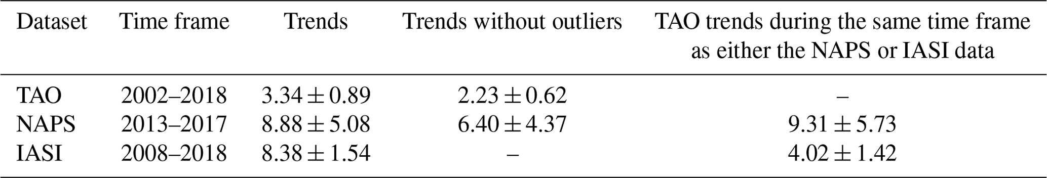
All three time series showed positive trends in NH₃ over Toronto: 3.34 ± 0.89 %/yr from 2002 to 2018 in the FTIR columns, 8.88 ± 5.08 %/yr from 2013 to 2017 in the surface in situ data, and 8.38 ± 1.54 %/yr from 2008 to 2018 in the IASI columns. To assess the representative scale of the FTIR NH₃ columns, correlations between the datasets were examined. The best correlation between FTIR and IASI was obtained with coincidence criteria of ≤25 km and ≤20 min, with r=0.73 and a slope of 1.14 ± 0.06. Additionally, FTIR column and in situ measurements were standardized and correlated. Comparison of 24 d averages and monthly averages resulted in correlation coefficients of r=0.72 and r=0.75, respectively, although correlation without averaging to reduce high-frequency variability led to a poorer correlation, with r=0.39.

The GEOS-Chem model, run at 2^∘ × 2.5^∘ resolution, was compared to FTIR and IASI to assess model performance and investigate the correlation of observational data and model output, both with local column measurements (FTIR) and measurements on a regional scale (IASI). Comparisons on a regional scale (a domain spanning 35 to 53^∘ N and 93.75 to 63.75^∘ W) resulted in r=0.57 and thus a coefficient of determination, which is indicative of the predictive capacity of the model, of r²=0.33, but comparing a single model grid point against the FTIR resulted in a poorer correlation, with r²=0.13, indicating that a finer spatial resolution is needed for modeling NH₃.

1 Introduction

Ammonia (NH₃) in the atmosphere plays an important role in the formation of nitrates and ammonium salts, is a major pollutant, and is known to be involved in numerous biochemical exchanges affecting all ecosystems (Erisman et al., 2008; Hu et al., 2014). As one of the main sources of reactive nitrogen in the atmosphere, NH₃ is also associated with acidification and eutrophication of soils and surface waters, which can negatively affect biodiversity (Vitousek et al., 1997; Krupa, 2003; Bobbink et al., 2010). Furthermore, NH₃ reacts with nitric acid and sulfuric acid to form ammonium salts, which are known to account for a large fraction of inorganic particulate matter (Schaap et al., 2004; Schiferl et al., 2014; Pozzer et al., 2017) and are thought to contribute to smog and haze (Liu et al., 2019; Wielgosiński and Czerwińska, 2020). Understanding how particulate matter forms is helpful in addressing air quality concerns (Schiferl et al., 2014), as particulate matter, especially that smaller than 2.5 µm (PM_2.5), poses serious health hazards affecting life expectancy in the United States (Pope et al., 2009) and globally (Giannadaki et al., 2014).

Due to the negative impacts NH₃ can have on public health and the environment, NH₃ emissions are regulated in some parts of the world (e.g., the 1999 Gothenburg Protocol to Abate Acidification, Eutrophication and Ground-level Ozone). However, global NH₃ emissions are increasing (Warner et al., 2016; Lachatre et al., 2019), and this has been attributed to increases in agricultural livestock numbers and increased nitrogen fertilizer usage (Warner et al., 2016). In addition, as the world population continues to grow and the demand for food rises, NH₃ emissions are expected to further increase (van Vuuren et al., 2011). Observations show increasing an abundance of atmospheric NH₃, particularly in the eastern United States, where trends as high as 12 % annually were observed (Yu et al., 2018). Yu et al. (2018) concluded that the increase in NH₃ abundance was in part due to decreasing SO₂ and NO_x (NO + NO₂), owing to more stringent emissions regulations. SO₂ and NO_x are precursors to acidic species (sulfuric and nitric acid, respectively) that react with NH₃, and thus their abundances in the atmosphere determine the amount of NH₃ that stays in the gaseous phase.

Atmospheric NH₃ is rapidly removed by wet and dry deposition as well as by heterogeneous reactions with acids in the atmosphere, and thus it has a relatively short lifetime ranging from a few hours to a few days (Galloway et al., 2003; Dammers et al., 2019). NH₃ lifetime may be longer for certain cases, such as biomass burning emissions that inject NH₃ into the free troposphere (Höpfner et al., 2016), attenuating depositional and chemical losses, although physical and chemical mechanisms that lead to the transport of NH₃ in biomass burning plumes over long distances remain uncertain (Lutsch et al., 2016, 2019). Dependence of PM_2.5 formation on NH₃ over urban areas also remains uncertain, and atmospheric chemical transport models have difficulty simulating NH₃ and PM_2.5 (e.g., Van Damme et al., 2014b; Fortems-Cheiney et al., 2016; Schiferl et al., 2016; Viatte et al., 2020).

Modeled NH₃ can be used to supplement observations (Liu et al., 2017). However, ground-level NH₃ abundances are poorly modeled, due to coarse model resolution, uncertain emissions inventories, and the simplification of chemistry schemes (Liu et al., 2017). Additionally, long-term trend analyses using models have been sparse (Yu et al., 2018). Representative measurements of NH₃ on both local and regional scales, as well as their spatiotemporal variabilities, are needed to better understand and model NH₃ and PM_2.5 formation (Viatte et al., 2020).

Toronto is the most populous city in Canada, and NH₃, along with other pollutants, is monitored by several instruments. In particular, the Fourier transform infrared (FTIR) spectrometer situated at the University of Toronto Atmospheric Observatory (TAO) has been making regular measurements since 2002. It is located in downtown Toronto, where local point sources (i.e., vehicle emissions) and nearby agricultural emissions, are major sources of NH₃ (Zbieranowski and Aherne, 2012; Hu et al., 2014; Wentworth et al., 2014). Toronto is also regularly affected by biomass burning plumes transported from the USA and other regions of Canada (Griffin et al., 2013; Whaley et al., 2015; Lutsch et al., 2016, 2020). As such, the time series of total column NH₃ measured at TAO exhibits long-term trends and pollution episodes. Toronto also has in situ (surface) measurements of NH₃ (Hu et al., 2014), made by Environment and Climate Change Canada. A study by Hu et al. (2014) investigating NH₃ in downtown Toronto has shown that greenery within the city, where chemical fertilizers are commonly used, is an important source of NH₃ when temperatures are above freezing and that potential sources at temperatures below freezing have yet to be investigated. Additionally, recent studies have shown the increased capacity for satellite-based instruments to measure spatial and temporal distributions of NH₃ total columns at global (Van Damme et al., 2014a; Warner et al., 2016; Shephard et al., 2020), regional (Van Damme et al., 2014b; Warner et al., 2017; Viatte et al., 2020), and point-source scales (Van Damme et al., 2018; Clarisse et al., 2019a; Dammers et al., 2019).

In this study, NH₃ variability over Toronto is investigated using ground-based FTIR data, in situ measurements, and satellite-based observations from the Infrared Atmospheric Sounding Interferometer (IASI). This study is a part of the AmmonAQ project, which investigates the role of NH₃ in air quality in urban areas. Trends in the NH₃ time series and their statistical significance are determined, and the GEOS-Chem model is also used to supplement and compare to observations. Additionally, correlations between FTIR and IASI, FTIR and in situ, in situ and IASI, FTIR and model data, and IASI and model data on a regional scale are analyzed to assess the representativeness of the FTIR NH₃ measurements.

The paper is organized as follows: Section 2 describes the FTIR retrieval methodology, the in situ and satellite data, the GEOS-Chem model, and the analysis methodologies. Section 3 presents the trend analysis of the FTIR, in situ, and IASI measurements, the results of the correlation studies, and an analysis of the representativeness of the FTIR NH₃. Section 4 presents the evaluation of the GEOS-Chem model, and conclusions are provided in Sect. 5.

2 Datasets and methods

2.1 FTIR measurements

Ground-based NH₃ total columns used in this study were retrieved from infrared solar absorption spectra recorded using an ABB Bomem DA8 FTIR spectrometer situated at the University of Toronto Atmospheric Observatory in downtown Toronto, Ontario, Canada (43.66^∘ N, 79.40^∘ W; 174  m a.s.l.). This instrument has been making measurements since mid-2002, and trace gas measurements are contributed to the Network for Detection of Atmospheric Composition Change (NDACC; http://www.ndaccdemo.org/, last access: 2 February 2021) (De Mazière et al., 2018). The DA8 has a maximum optical path difference of 250 cm, with a maximum resolution of 0.004 cm⁻¹, and is equipped with a KBr (700–4300 cm⁻¹) beam splitter. While the FTIR is equipped with both InSb and HgCdTe (MCT) detectors, NH₃ profiles were retrieved using the MCT detector, which is responsive from 500–5000 cm⁻¹. The DA8 is coupled to an active sun tracker, which was manufactured by Aim Controls. The tracker is driven by two Shinano stepper motors on elevation and azimuth axes. The active tracking was provided by four photo-diodes from 2002–2014. This was upgraded to a camera and solar-disk-fitting system in 2014 (Franklin, 2015). Detailed specifications of the system can be found in Wiacek et al. (2007). Due to the nature of solar-pointing FTIR spectroscopy, the measurements are limited to sunny days, resulting in gaps in the time series. Measurements are typically made on 100–150 d per year.

The FTIR at TAO uses six filters recommended by the NDACC Infrared Working Group (IRWG) and measures spectra through each filter in sequence. NH₃ profiles were retrieved using two microwindows in the 930.32–931.32 cm⁻¹ and 966.97–967.675 cm⁻¹ spectral regions. Interfering species include H₂O, O₃, CO₂, N₂O, and HNO₃. The solar absorption spectra recorded by the DA8 were processed using the SFIT4 retrieval algorithm (https://wiki.ucar.edu/display/sfit4/, last access: 1 November 2020). SFIT4 uses the optimal estimation method (OEM) (Rodgers, 2000) and works by iteratively adjusting the target species volume mixing ratio (VMR) profile until the difference between the calculated spectrum and the measured spectrum and the difference between the retrieved state vector and the a priori profile is minimized. The calculated spectra use spectroscopic parameters from HITRAN 2008 (Rothman et al., 2009) and atmospheric information (temperature and pressure profiles for any particular day) provided by the US National Centers for Environmental Prediction (NCEP). A priori VMR profiles were based on the a priori profile used at the NDACC site in Bremen (Dammers et al., 2015), which was obtained from balloon-based measurements (Toon et al., 1999). The NH₃ retrieval methodology used at TAO is described in detail in Lutsch et al. (2016).

Uncertainties in the retrievals include measurement noise and forward model errors. Smoothing errors that arise due to the discretized vertical resolution were not included, to conform to NDACC standard practice. Measurement noise error includes errors due to uncertainties in instrument line shape, interfering species, and wavelength shifts. Uncertainties in line intensity and line widths were calculated based on HITRAN 2008 errors. Error analysis was performed on all retrievals (following Rodgers, 2000); the resulting errors were grouped into random and systematic uncertainties and added in quadrature. The resulting mean uncertainties averaged over the entire time series were 12.9 % and 11.8 % for random and systematic errors, respectively, for a total average error of 18.8 % on the NH₃ total columns. The mean degrees of freedom for signal (DOFSs) averaged over the 2002–2018 time series was 1.10.

2.2 In situ measurements

To complement the FTIR total column NH₃ measurements, the publicly available in situ data obtained by Environment and Climate Change Canada (ECCC) as a part of the National Air Pollution Surveillance Program (NAPS) were used (http://maps-cartes.ec.gc.ca/rnspa-naps/data.aspx, last access: 1 November 2020). The data span December 2013 to April 2017, with a sampling frequency of 1 in 3 d. The sampling interval is 24 h, from 00:00 to 24:00 local time, and samples were collected with a Met One SuperSASS-Plus Sequential Speciation Sampler. The detection limit is 0.6 ppb (Yao and Zhang, 2013). The integrated samples were brought back to the lab for analysis (Yao and Zhang, 2016). While errors are not reported in the dataset, the uncertainty is 10 % when the NH₃ VMR is between 3 to 20 ppb (Hu et al., 2014). The instrument is situated less than 500 m away from the FTIR, at 43.66^∘ N, 79.40^∘ W and 63 m a.s.l..

2.3 IASI measurements

IASI is a nadir-viewing FTIR spectrometer on board the MetOp-A, MetOp-B, and MetOp-C polar-orbiting satellites, operated by the European Organization for the Exploitation of Meteorological Satellites (EUMETSAT), which have been operational since 2006, 2012, and 2018, respectively. The MetOp A, B, and C satellites are in the same polar orbit. For all three satellites, IASI makes measurements at 09:30 and 21:30 mean local solar time for the descending and ascending orbits. IASI records spectra in the 645–2760 cm⁻¹ spectral range at a resolution of 0.5 cm⁻¹, with apodization. IASI can make off-nadir measurements of up to 48.3^∘ on either side of the track, leading to a swath of about 2200 km. At nadir, the field of view is a 2 × 2 matrix of pixels, each with a 12 km diameter (Clerbaux et al., 2009).

The IASI NH₃ total columns (IASI ANNI-NH3-v3) are retrieved using an artificial neural network retrieval algorithm, with ERA5 meteorological reanalysis input data (Van Damme et al., 2017; Franco et al., 2018). Due to this retrieval scheme, there are no averaging kernels nor vertical sensitivity information for the retrieved columns (Van Damme et al., 2014a). Details of the retrieval scheme and error analysis can be found in Whitburn et al. (2016) and Van Damme et al. (2017). IASI-A and IASI-B NH₃ were combined and used in this study, as this allows for a longer time series and more data points for robust analysis. The retrieved columns of NH₃ from both satellites have been shown to be consistent with each other (Clarisse et al., 2019b; Viatte et al., 2020).

2.4 GEOS-Chem

The GEOS-Chem (v11-01) global chemical transport model (CTM) (http://geos-chem.org, last access: 1 November 2020) was used in this study to supplement and compare to observational data. The model was run at 2^∘ ×  2.5^∘ resolution (latitude × longitude) using MERRA2 (Modern-Era Retrospective analysis for Research and Applications, Version 2) meteorological fields (Molod et al., 2015) and the EDGAR v4.2 emissions database (Janssens-Maenhout et al., 2019) for anthropogenic emissions. For NH₃, EDGAR v4.2 and GEIA were used as global inventories, with GEIA providing the natural source of NH₃ (Bouwman et al., 1997; Olivier et al., 1998; Croft et al., 2016). The global inventories were replaced with the US EPA National Emission Inventory for 2011 (NEI11; https://www.epa.gov/air-emissions-inventories/2011-national-emissions-inventory-nei-data, last access: 1 November 2020) in the United States and by the Criteria Air Contaminants (CACs) from the National Pollutant Release Inventory in Canada (https://www.ec.gc.ca/inrp-npri/, last access: 1 November 2020). The NEI11 emissions were scaled between the years 2006–2013, whereas the CAC NH₃ emissions used 2008 as the base year, with no scaling applied. The NEI11 emissions were hourly, whereas the CAC emissions were monthly. The GEOS-Chem model includes a detailed tropospheric oxidant chemistry and aerosol simulation (e.g., H₂SO₄–HNO₃–NH₃ simulation) (Park et al., 2004). For SO₂ and NO, which can lead to the formation of sulfates and nitrates that influence NH₃ uptake to aerosols, the EDGAR and CAC (for Canada; https://www.ec.gc.ca/inrp-npri/, last access: 1 November 2020) inventories were used. NH₃ gas–aerosol partitioning is calculated using the ISORROPIA II model (Fountoukis and Nenes, 2007). Chemistry and transport are calculated with 20 and 10 min time steps, respectively. The model was spun up for 1 year, and output was saved every hour from 2002 to 2018.

2.5 TAO FTIR and IASI comparison

To assess the representative spatial and temporal scale of TAO FTIR NH₃ columns, the NH₃ total column measurements around Toronto made by IASI were compared to TAO FTIR total columns and modeled NH₃ columns (see Sect. 3.3). As NH₃ shows high spatiotemporal variability, several definitions of coincident measurements were used in this study, with spatiotemporal criteria of varying strictness. As NH₃ concentrations can vary significantly during the day, the temporal coincidence criterion was chosen to be ≤90 min (Dammers et al., 2016). In addition, values of ≤60, 45, 30, and 20 min were also tested. For spatial coincidence criteria, ≤25 (Dammers et al., 2016), 30, 50, and 100 km were tested. For each criterion, correlations (both r and slope) were calculated. This analysis was used to evaluate the spatial and temporal scales represented by the TAO FTIR NH₃ columns.

2.6 Trend analysis and identifying pollution events

With 16 years of data, relatively long-term trends of TAO FTIR column time series can be examined. While a trend analysis simply using monthly averages is possible (Angelbratt et al., 2011), a more sophisticated method of fitting Fourier series of several orders was utilized in this study (Weatherhead et al., 1998). Bootstrap resampling was utilized to derive the confidence interval of the trends (Gardiner et al., 2008). A Q value (the number of bootstrap resampling ensemble members generated for statistical analysis) of 5000 was used (Gardiner et al., 2008). An additional analysis to determine the number of years of measurements needed to give the derived trend statistical significance (2σ confidence) was also conducted, following Weatherhead et al. (1998). This analysis takes into account the need for longer time series to identify trends in data that are autocorrelated (as are atmospheric observations). It should be noted that a major limitation of this analysis is that it assumes that data are collected at regular intervals, while TAO measurements are made at irregular intervals (due to the need for sunny conditions). For this reason, the confidence intervals derived from bootstrap resampling are a more robust method of error analysis, in the case of TAO data. However, as pointed out by Weatherhead et al. (1998), failing to take into account the autocorrelation of the noise can lead to underestimations of actual uncertainty, and for this reason, both bootstrap resampling and the Weatherhead method were used in this study. These techniques were combined to assess the intra- and inter-annual trends of NH₃ derived from TAO measurements, including a linear trend of the NH₃ total column along with its uncertainties and statistical significance. This analysis was also applied to the NAPS in situ and IASI data.

The Fourier fit was used to identify NH₃ enhancements, following Zellweger et al. (2009). This analysis is done by taking the negative residuals of the fit (i.e., measured values smaller than fitted values), mirroring them, and calculating the standard deviation (σ) of the mirrored residuals. Any measurements that are 2σ above the fit are considered enhancements. This analysis reduces biases in the spread due to enhancements by mirroring the negative residuals.

In this study, Fourier series of order 3 were utilized for all analyses. An analysis was done by comparing Fourier series fits of order 1 to 7 and checking for overfitting by running the residuals of the fit through a normality test (the Kolmogorov–Smirnov test). While overfitting was not observed at higher orders, higher orders did not give more statistically significant trends, so order 3 was chosen.

3 Results and discussion

3.1 FTIR measurements

The TAO FTIR total column time series of NH₃ is shown in Fig. 1. The purple points indicate enhancements, and the trends (with and without outliers) are shown as red and cyan lines, respectively. The trend from 2002 to 2018 was found to be 3.34 ± 0.89 %/yr and 2.23 ± 0.62 %/yr (2σ confidence interval from bootstrap resampling), with and without outliers, respectively (see Table 2). The number of years of measurements needed for the trend to be statistically (2σ) significant was found to be 33.8 years and 29.3 years, with and without enhancement events, respectively. Due to the irregular FTIR measurement intervals, these numbers may not represent the true significance of the trends and should be regarded as best estimates of the significance of the observed trend. The lower magnitude of the upward trend in the analysis without enhancement values indicates that the intra-annual variability of NH₃ is increasing. This is also evident when comparing the mean total column and standard deviations from, for example, the periods 2002–2005 and 2015–2018. In the former period, the mean NH₃ total column and standard deviation (1σ) were 5.94 ± 5.14 ×10¹⁵ molecules/cm², while in the latter time frame, they were 8.13 ± 7.88 ×10¹⁵ molecules/cm². The observed trend with the FTIR is comparable to a study by Warner et al. (2017), who observed an increasing NH₃ trend of 2.61 %/yr over the United States from 2002 to 2016 using data from the Atmospheric Infrared Sounder (AIRS) satellite-based instrument.

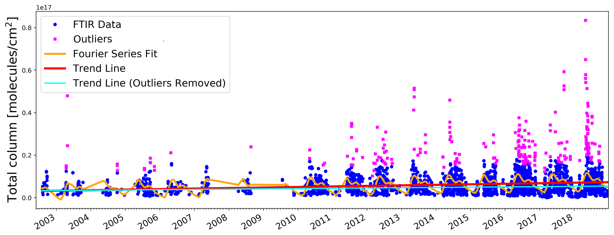
Figure 1 Time series of TAO FTIR NH₃ total columns from 2002 to 2018 with third-order Fourier series fit and linear trends.

Figure 2 shows the annual cycle of the FTIR NH₃ total columns, color-coded by year, along with the monthly averages and ±2σ. FTIR NH₃ columns have a maximum in May with a monthly total column average of 13.14 ± 11.69 ×10¹⁵ molecules/cm², largely due to agricultural and soil emissions increasing in spring and summer (Hu et al., 2014; Dammers et al., 2016), and a minimum in January with a monthly total column average of 2.11 ± 1.81 ×10¹⁵ molecules/cm². The lower NH₃ columns during winter months may be due to lower temperatures favoring the formation of NH₄NO₃ (Li et al., 2014). The seasonal cycle observed with the FTIR is consistent with findings by Van Damme et al. (2015b), who observed maximum NH₃ columns over the central United States during March–April–May (MAM). The mean NH₃ total column across the entire FTIR time series was 7.53 ± 7.10 ×10¹⁵ molecules/cm². These values are higher than remote areas, such as Eureka (located at 80.05^∘ N, 86.42^∘ W), where the highest monthly average was 0.279×10¹⁵ molecules/cm², in July (Lutsch et al., 2016). However, the TAO FTIR NH₃ total columns are far below values observed by the FTIR in Bremen (located at 53.10^∘ N, 8.85^∘ E), which saw values in the range of $\sim \mathrm{100}\times {\mathrm{10}}^{\mathrm{15}}$ molecules/cm² (Dammers et al., 2016). Monthly mean NH₃ columns are listed in Table 1.

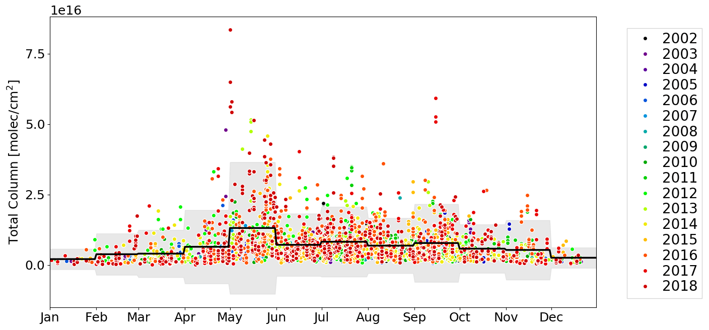
Figure 2 TAO FTIR NH₃ total columns plotted from January to December for 2002 to 2018. Monthly averages and ±2σ are indicated by the black line and shading, respectively.

Table 1 Monthly mean (1σ in parenthesis) NH₃ total columns of the TAO FTIR (2002–2018).

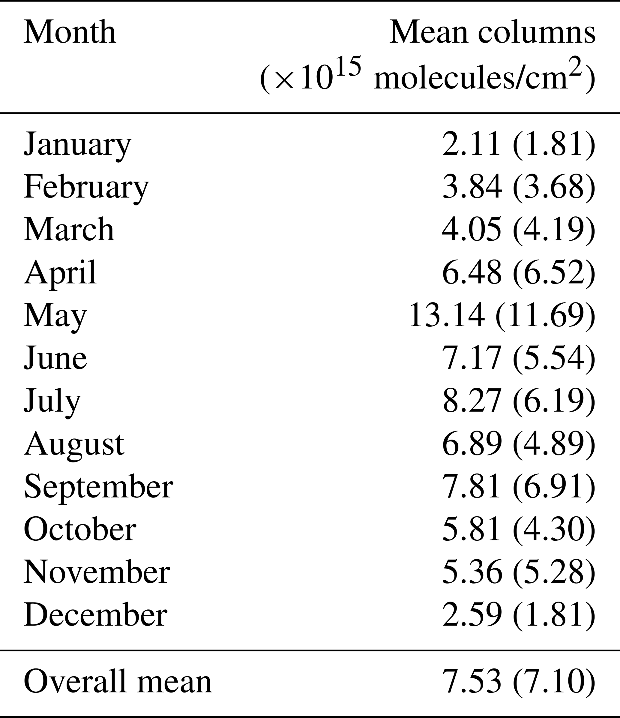
Table 2 Comparison of NH₃ trends and 2σ confidence intervals observed in Toronto. All trends are in %/year.

3.2 NAPS measurements

The NAPS in situ NH₃ time series is shown in Fig. 3. The purple points indicate enhancements, and trend lines with and without these outliers are shown as the red and cyan lines, respectively. The trend line was found to have a slope of 8.88 ± 5.08 %/yr and 6.40 ± 4.37 %/yr (2σ confidence interval from bootstrap resampling), with and without outliers, respectively. The number of years needed for this trend to be 2σ significant was 8.4 years for both. Since NAPS data have very regular measurement intervals (once every 3 d), they are well suited for this trend significance analysis. Given that NAPS data only span 3 years and 5 months and given that 8.4 years of measurements are needed for 2σ confidence in the observed trend, it is uncertain if the increase in NH₃ levels is a definitive trend. For comparison, analysis of TAO FTIR NH₃ total columns during the same time period resulted in trends of 9.31 ± 5.73 %/yr and 7.42 ± 4.48 %/yr, with and without outliers, respectively.

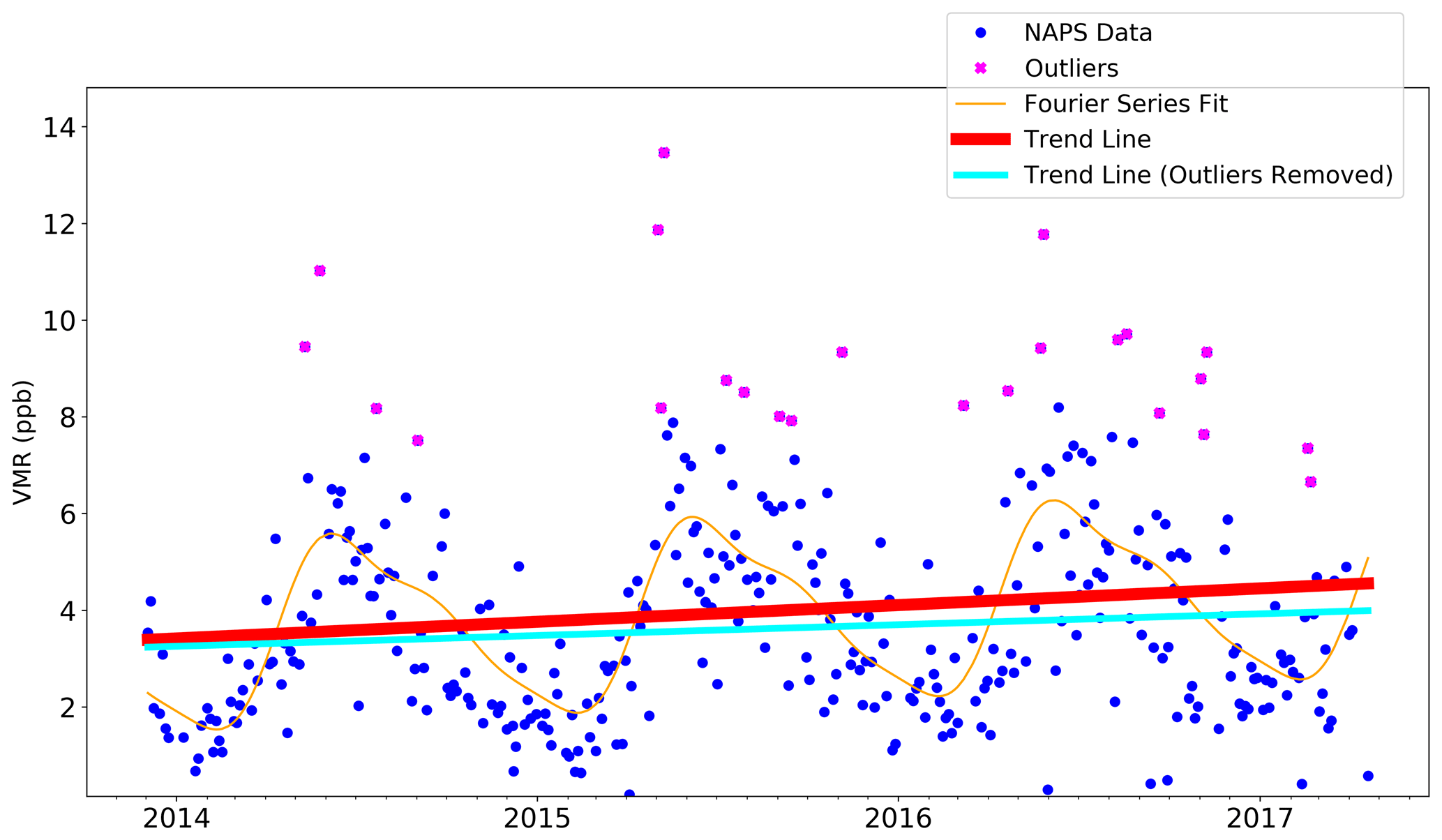
Figure 3 Time series of NAPS NH₃ surface VMR from 2013 to 2017 with third-order Fourier series fit and linear trends.

The in situ NH₃ VMRs were compared to the TAO FTIR columns by standardizing both measurements, following Eq. (1) of Viatte et al. (2020):

$$\begin{array}{}\text{(1)}& X_{\text{standardized}}^i={\displaystyle \frac{X_i-{\mathit{\mu }}_X}{{\mathit{\sigma }}_X}},\end{array}$$

where X is the dataset, indexed by i, μ is the mean, and σ is the standard deviation of the dataset. The standardized dataset is centered around zero and normalized by the standard deviation of the measurements. As the standardized dataset is unitless, it allows for comparison between different measurements in different units. In this study, the TAO FTIR NH₃ total columns were used because the DOFS for the retrieval was around 1 (mean DOFS of the entire time series was 1.10), meaning there is only about one piece of vertical information in these measurements.

Standardized FTIR and NAPS NH₃ are plotted in Fig. 4a. Monthly averages and monthly standard deviations are shown in Fig. 4b. The two measurements show similar seasonal cycles, with a maximum in May and a minimum in December and January. There is a smaller secondary peak in November for both measurements. This may be due to late-season fertilizer application and cover crop growth. The Ministry of Agriculture, Food and Rural Affairs of Ontario recommends applying fertilizer in spring and fall (Munroe et al., 2018). Correlation between the two datasets can be seen in Fig. 5a, where each NAPS measurement is plotted against the average of FTIR measurements on that day (if any measurements are available). This simple comparison does not show a strong correlation, with r=0.51 and slope = 0.501. However, resampling the measurements by 15 d averages (Fig. 5b), 18 d averages (Fig. 5c), 24 d averages (Fig. 5d), and by monthly averages (Fig. 5e) shows much stronger correlations. Resampling to 15 d averages shows better correlation with r=0.63 and a larger slope = 0.707. Averaging to every 18 and 24 d leads to r=0.68 and 0.72, respectively. Monthly averages show the highest correlation with r=0.75 and a slope = 0.758. This indicates that the FTIR and NAPS see similar low-frequency variabilities (period of 2 weeks or longer) in NH₃.

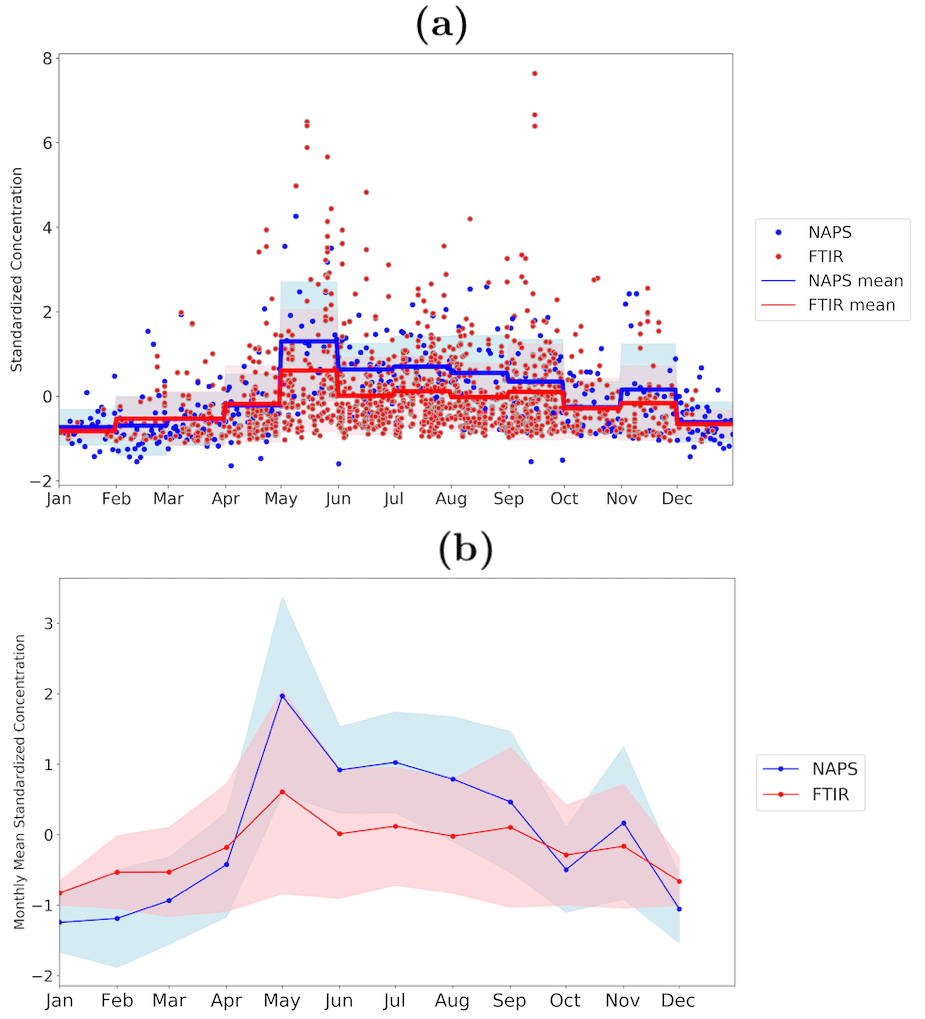
Figure 4 (a) Standardized FTIR total column and NAPS surface VMR of NH₃ plotted from January to December. Monthly averages and ±1σ are indicated by the red and blue lines and shading for the FTIR and NAPS, respectively. (b) The standardized FTIR NH₃ total column (red) and NAPS surface NH₃ VMR (blue) monthly average lines with their respective ±1σ (shading).

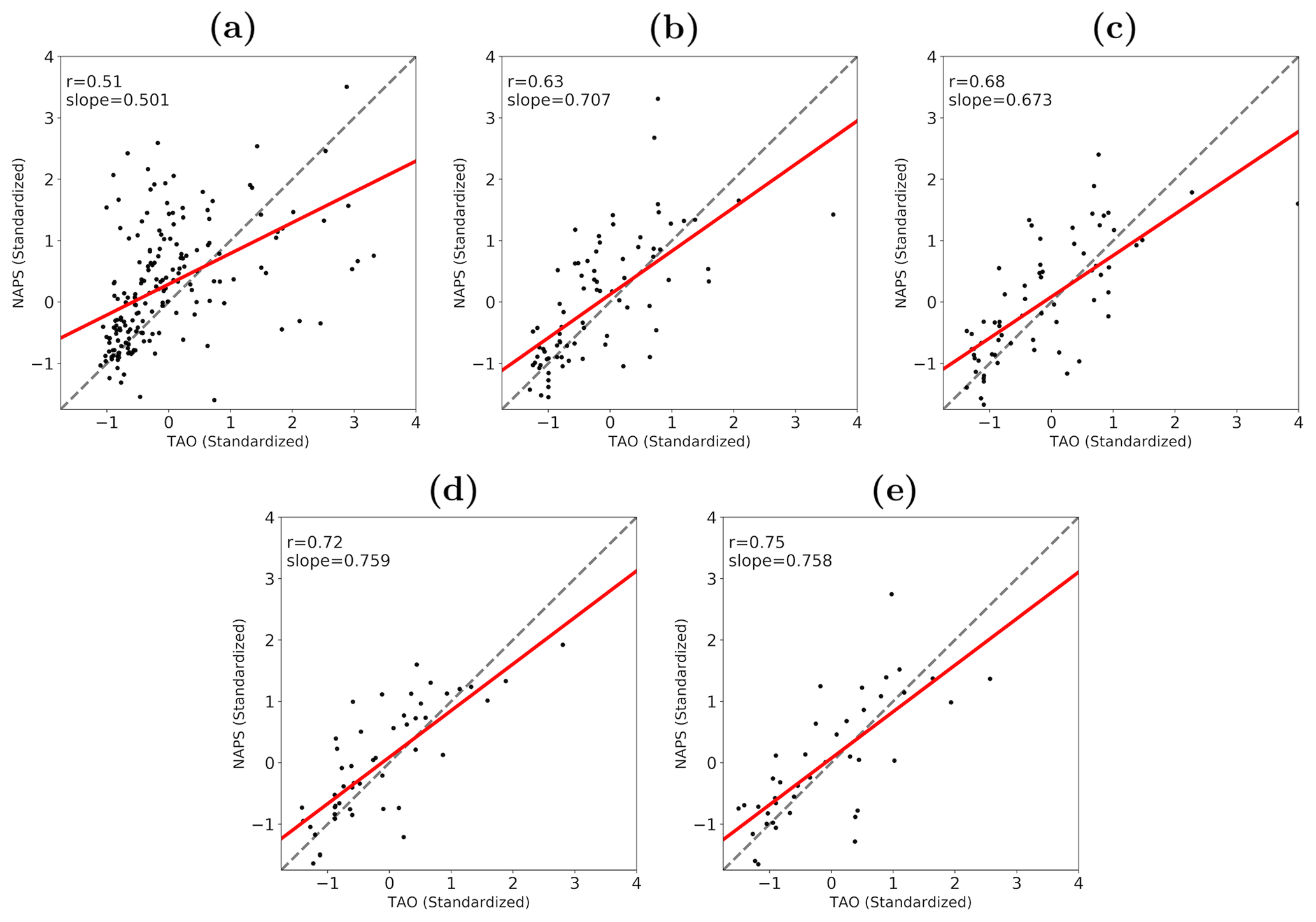
Figure 5 Standardized NAPS NH₃ surface VMR plotted against standardized FTIR NH₃ total column. (a) The raw comparison, where the closest daily average FTIR measurement is plotted for each NAPS observation if there are any within 72 h. FTIR and in situ resampled to (b) 15 d, (c) 18 d, (d) 24 d, and (e) monthly averages. The dashed lines indicate slope = 1, and the red lines indicate the fit to the data.

It should be noted that a bias would be expected to be observed between the FTIR and NAPS data, as the FTIR can only make measurements during sunny conditions, while NAPS data are 24 h averages, made once every 3 d. This means that NAPS data include observations made during nighttime and rainy conditions. This is noteworthy, as surface NH₃ concentrations may be affected by diurnal variability in the planetary boundary layer height. Temperature may also affect NH₃ enhancement events. When coincident datasets were analyzed for enhancements, 3 d showed simultaneous enhancements (25 May 2014, 23 May 2016, 26 May 2016). On all 3 d, the daily average temperature (measured by the TAO weather station) was higher than the corresponding monthly average: 19.3 ± 2.8 ^∘C (uncertainties indicate 1 standard deviation) on 25 May 2014 vs. May 2014 monthly mean of 13.8 ^∘C and 19.6 ± 3.4 and 21.2 ± 2.8 ^∘C for 23 May and 26 May 2016, respectively, vs. the May 2016 monthly mean of 14.1 ^∘C. This is unsurprising, given that increased NH₃ is correlated with higher temperatures (e.g., Meng et al., 2011). Since the FTIR can only make measurements on sunny days, its measurements may be biased high compared to NAPS, which makes measurements regardless of weather.

3.3 IASI measurements

The time series of IASI NH₃ total columns (2008 to 2018) within 50 km of TAO is shown in Fig. 6. The trend of these IASI measurements is 8.38 ± 1.43 %/yr, where the error indicates the 2σ confidence interval obtained by bootstrap resampling analysis. The Weatherhead et al. (1998) method for finding the statistical significance of this trend was not utilized here, as the analysis requires calculating the autocorrelation of data, which is not possible given the spatially scattered dataset. For comparison, the TAO FTIR trend over the same period is 4.02 ± 1.42 %/yr.

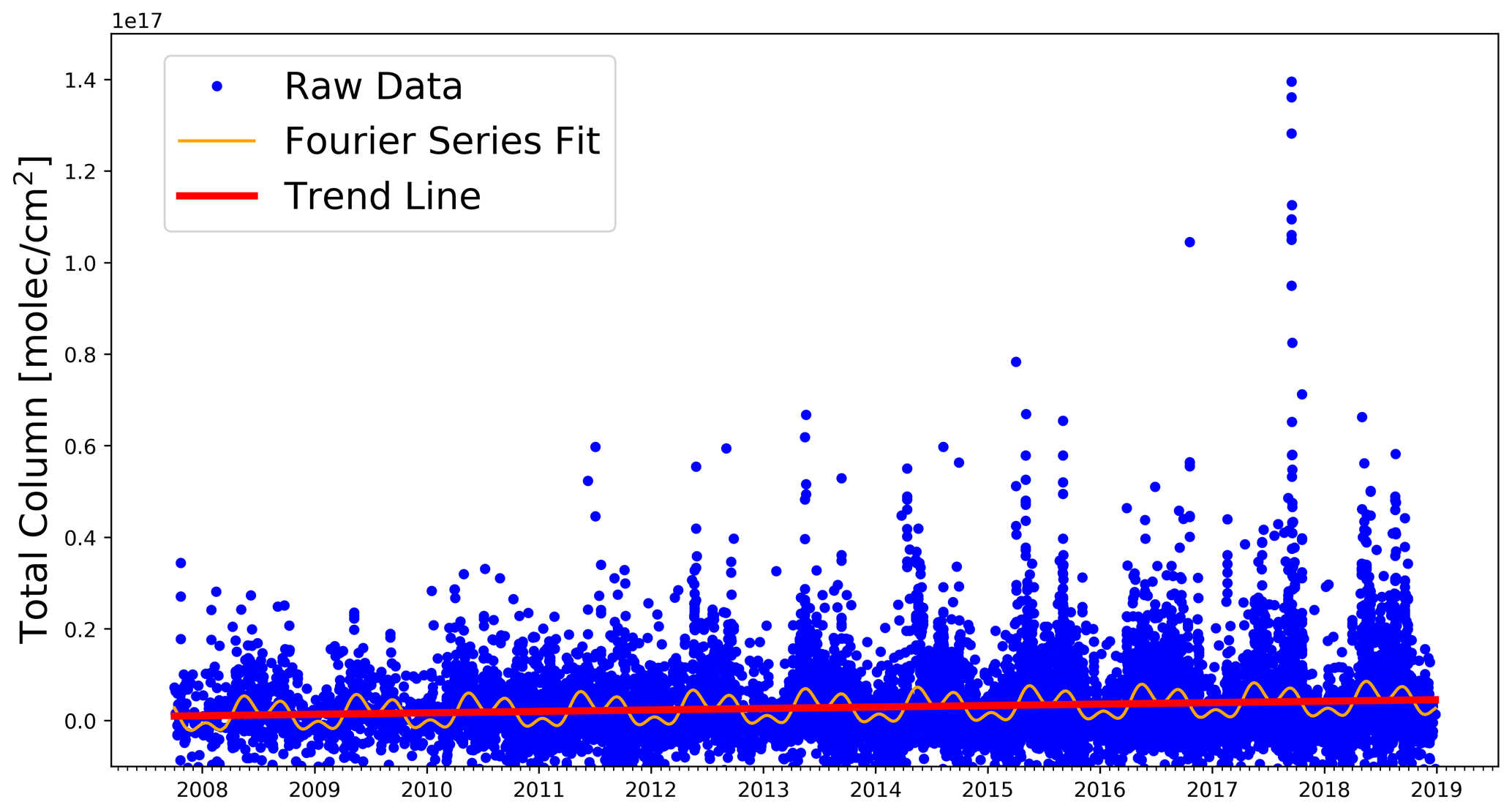
Figure 6 Time series of IASI NH₃ total columns measured within 50 km of TAO. The third-order Fourier series fit and the trend line are shown in orange and red, respectively.

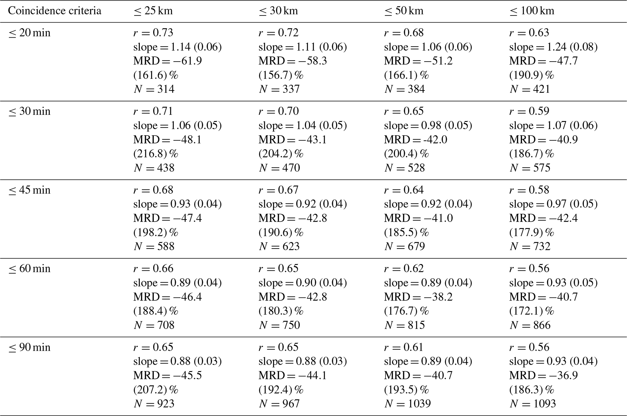
The correlations between IASI and TAO FTIR NH₃ columns for the various coincidence criteria listed in Sect. 2.3 are shown in Table 3, along with the slopes, mean relative difference (MRDs), and total number of data points. The MRD was calculated by subtracting the TAO FTIR column from the IASI column, then dividing by the TAO FTIR column (Dammers et al., 2016). To maximize the number of coincident data points, no significant data filtering (e.g., filtering by relative errors) was performed. The criteria used by Dammers et al. (2016) (90 min, 25 km) show a correlation with r=0.65 and slope = 0.88 in this study, comparable to r=0.79 and slope = 0.84 reported by Dammers et al. (2016). The MRD was $-\mathrm{45.5}\pm \mathrm{207.2}$ % for this study, consistent with $-\mathrm{46.0}\pm \mathrm{47.0}$ % calculated by Dammers et al. (2016) for TAO FTIR data. The larger standard deviation of the MRD is most likely because the data used here were not filtered by relative errors. The best correlation was achieved when using measurements made within 20 min and within 25 km of each other, which resulted in r=0.73 and a slope of 1.14. Coincidence criteria of 20 min and 50 km gave r=0.68 and slope = 1.06. Criteria of 45 min and 50 km also show a correlation comparable to the 90 min, 25 km criteria, with r=0.64 and slope = 0.92. This suggests that TAO FTIR is a good indicator of NH₃ concentrations on a city-wide scale (∼50 km). This is also evident when looking at the correlation between TAO FTIR columns vs. daily averaged IASI measurements within 50 km, which had r=0.69, although the slope was smaller, at 0.82. The better correlations seen with the stricter temporal criteria suggest that NH₃ near Toronto exhibits high-frequency variability. The values obtained in this study are also comparable to recent findings by Tournadre et al. (2020), who compared NH₃ columns from an FTIR stationed in Paris to IASI NH₃ columns. With a 15 km and 30 min coincidence criteria, the FTIR in Paris showed a correlation of r=0.79 and slope = 0.73. The same study also found that the FTIR in Paris is capable of providing information about NH₃ variability at a “regional” scale (∼120 km) (Tournadre et al., 2020). Although not quantified in this study, the line-of-sight through the atmosphere (which changes throughout the day) may also affect the representative scale of ground-based solar-pointing FTIR observations. Additionally, the number of observations is relatively large for each criterion (e.g., N=923 for 90 min, 25 km, while N=679 for 45 min, 50 km), suggesting that the differences in correlation are not simply due to the differences in the number of data points. The correlation plots for 20 min/25 km, 90 min/25 km, 20 min/50 km, and 45 min/50 km are shown in Fig. 7a, 7b, 7c, and 7d, respectively. It should be noted that the slope was calculated through a simple linear least-squares regression. For comparison, an additional analysis was done propagating measurement uncertainty using the unified least squares procedure outlined by York et al. (2004) and yielded similar results, with a smaller slope for all cases due to the larger relative uncertainty on IASI measurements (∼68 % for IASI compared to ∼19 % for TAO FTIR).

Figure 7 Correlation plots for IASI vs. TAO FTIR NH₃ total columns, with coincidence criteria of (a) 20 min and 25 km, (b) 90 min and 25 km, (c) 20 min and 50 km, and (d) 45 min and 50 km. Data from 2008 to 2018 are plotted. Dashed lines indicate slope = 1, while the red lines are the lines of best fit. Error bars are the reported observational uncertainties.

Table 3 IASI vs. TAO FTIR correlation coefficient, slope (regression standard error in parenthesis), MRD (1σ rms in parenthesis) (in %), and number of data points, calculated for each TAO FTIR measurement, for varying spatial and temporal coincidence criteria.

IASI column and NAPS surface NH₃ were also compared in this study by converting to standardized data (see Eq. 1). Comparing the monthly means resulted in r=0.79 and slope = 0.79 when looking at IASI measurements made within 50 km of NAPS and r=0.74 and slope = 0.74 for 30 km. Without temporal averaging, no significant correlation was found (r≤0.27) for any spatial coincidence criteria. This is in line with findings from Van Damme et al. (2015a), where significant correlation was found when comparing monthly averaged surface and IASI measurements. Van Damme et al. (2015a) report r=0.28 when comparing IASI with an ensemble of surface observations over Europe and r as high as 0.81 and 0.71 for measurements made at Fyodorovskoye, Russia, and Monte Bondone, Italy, respectively. It should be noted that the comparisons in Van Damme et al. (2015a) were done by converting IASI NH₃ columns to surface concentration by using the same model used in the retrieval process, as opposed to the standardized dataset approach used in this study.

4 Comparison with GEOS-Chem

The NH₃ total column from the GEOS-Chem CTM model grid cell containing Toronto (grid center at 44^∘ N, 80^∘ W) is shown in Fig. 8a, along with TAO FTIR data. The correlation was obtained by comparing the hourly model data for each FTIR observation. Comparison with the FTIR was done with and without smoothing the model data with the FTIR averaging kernel and a priori profile (Rodgers and Connor, 2003). As smoothing the model data only resulted in differences of less than 1 %, the discussion here will focus on the unsmoothed dataset to be consistent with the comparison with IASI. While GEOS-Chem is able to capture the seasonal cycle seen with the FTIR, the correlation is not strong, with r=0.51 and the coefficient of determination, r², at 0.26 (see Fig. 9a). The calculated slope was 1.16. Both of these values are without smoothing the model data. Smoothing the data resulted in r²=0.28 and slope = 1.01 It is likely that the model is too coarse (the 2^∘ × 2.5^∘ grid box corresponds to approximately 220 km × 200 km), and the FTIR, while able to capture larger-scale variability in NH₃ than in situ observations, is not sensitive to observations at spatial scales of 100 km or larger. Given the short lifetime of NH₃, it is unsurprising to see large variability at these spatial scales.

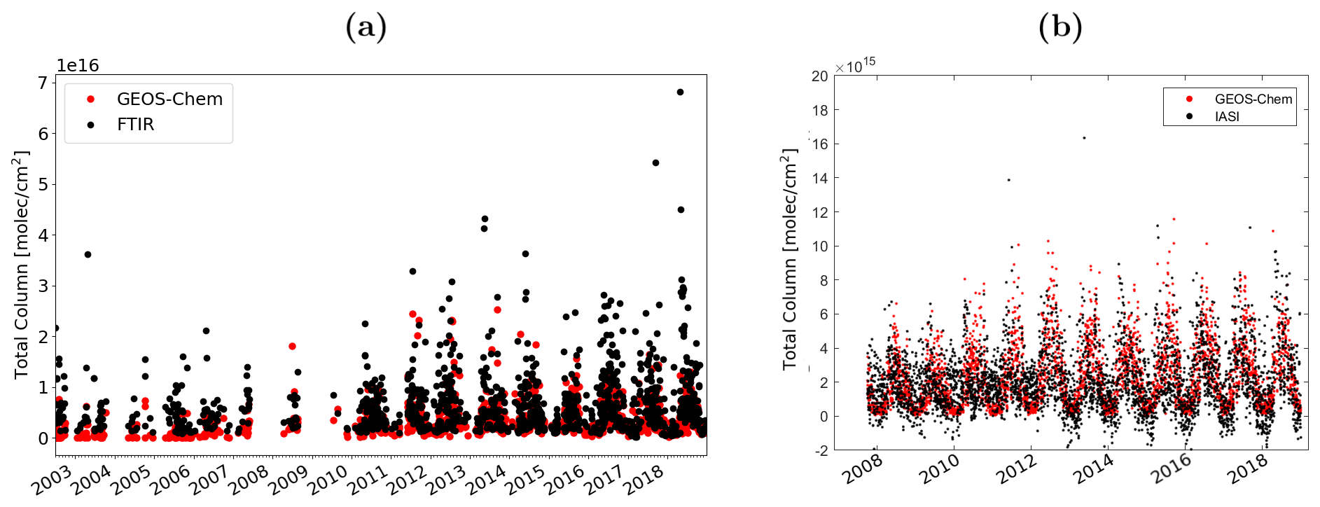
Figure 8 (a) GEOS-Chem and TAO FTIR NH₃ total columns from 2002 to 2018. GEOS-Chem data shown here were not smoothed with the FTIR averaging kernel and a priori profile. (b) GEOS-Chem and IASI NH₃ total columns (averaged over domain spanning from 35 to 53^∘ N and 93.75 to 63.75^∘ W) from 2008 to 2018.

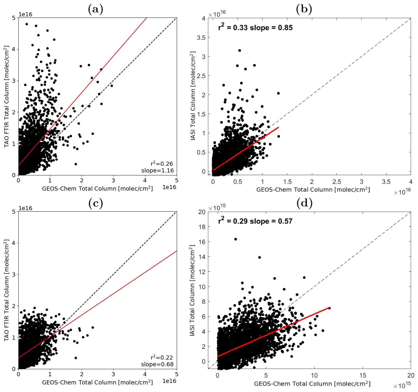
Figure 9 Correlation plots of (a) TAO FTIR vs. GEOS-Chem NH₃ total columns, (b) IASI vs. GEOS-Chem NH₃ total columns, (c) TAO FTIR with enhancement events removed vs. GEOS-Chem NH₃ total columns, and (d) IASI with enhancement events removed vs. GEOS-Chem NH₃ total columns. Data from 2002 to 2018 are plotted for TAO and data from 2008 to 2018 are plotted for IASI.

For comparison with IASI, a larger domain was chosen to assess the correlation of the model and satellite observations at a larger regional scale. Model grids spanning 35 to 53^∘ N and 93.75 to 63.75^∘ W were used for the analysis, as these grids capture Toronto, the Great Lakes, and the Atlantic Ocean coastline. The spatial coincidence was calculated by binning the IASI data into the grids of GEOS-Chem, and temporal coincidence was determined by calculating the mean overpass time in the domain and averaging the model data between 1 h before and 1 h after the mean overpass time. The time series (both GEOS-Chem and IASI were averaged over the domain), and correlation plots are shown in Figs. 8b and 9b, respectively. The correlation of GEOS-Chem against IASI is higher than GEOS-Chem against TAO FTIR, with r²=0.33 (see Fig. 9b). Removing enhancement events from observational data led to poorer correlation with GEOS-Chem, with r²=0.22 and r²=0.29 for the FTIR and IASI, respectively (see Fig. 9c and 9d). This is comparable to findings by Schiferl et al. (2016), who observed IASI and GEOS-Chem correlations (r) of 0.6–0.8 in the United States Great Plains and the Midwest during the summer. The slope was 0.85, meaning NH₃ is overestimated in GEOS-Chem when compared to IASI at this scale. Comparing GEOS-Chem and IASI for one grid cell over Toronto (same cell as the one used for comparison with TAO FTIR) resulted in a lower correlation, at r²=0.13. These results suggest GEOS-Chem is able to model NH₃ on larger regional scales but a finer resolution is needed for better comparison with smaller regions. In addition, while the modeled NH₃ was overestimated in comparison with IASI over a larger regional domain, the comparison for the single grid box over Toronto resulted in slope = 2.44, meaning the model underestimated NH₃ in this smaller region, which may indicate underestimation of local NH₃ sources near Toronto in the model. This can be contrasted with recent findings by Van Damme et al. (2014b), who observed an overall underestimation of NH₃ in the LOTOS-EUROS model over Europe when compared to IASI. In a 4-year period from 2008 to 2011 over the Netherlands, for example, IASI NH₃ columns are as high as 6.5 mg/m², while the modeled NH₃ go up to 5.2 mg/m² (Van Damme et al., 2014b).

5 Conclusions

The FTIR spectrometer situated in downtown Toronto, Ontario, Canada, has been used to obtain a 16-year time series of total columns of NH₃. These columns were compared to other NH₃ observations (IASI column and NAPS in situ surface VMR) and GEOS-Chem model data. Analysis of the FTIR NH₃ columns showed an upward annual trend of 3.34 ± 0.89 % and 2.23 ±  0.62 % over the period 2002–2018, with and without outliers, respectively. The larger trend with outliers included, along with a larger variance in the total column measurements in the later years, suggests that NH₃ enhancements are becoming more frequent and seasonal variability is increasing. These values are in agreement with trends observed by other studies. For example, Warner et al. (2017) observed a trend of 2.61 %/yr from 2002 to 2016 over the USA using data from the Atmospheric Infrared Sounder (AIRS) aboard NASA's Aqua satellite, and Yu et al. (2018) derived surface NH₃ trends of ∼5 % and ∼5 %–12 % in the western and eastern United States from 2001 to 2016, respectively, using GEOS-Chem modeled NH₃.

Similar analysis of the NAPS in situ time series showed that NH₃ at the surface is also increasing, with an annual increase of 8.88 ± 5.08 % and 6.40 ± 4.37 % calculated with and without outliers, respectively. The FTIR total columns during the same period showed trends of 9.31 ± 5.73 %/yr and 7.42 ± 4.48 %/yr with and without outliers, respectively. The FTIR and NAPS comparisons showed that the FTIR columns are well correlated with surface NH₃ when resampled to monthly means to reduce high-frequency variability.

IASI NH₃ total columns measured within 50 km of TAO exhibited an annual trend of 8.38 ± 1.54 %/yr from 2008 to 2018. For comparison, TAO FTIR NH₃ total columns over the same period showed a trend of 4.02 ± 1.42 %/yr. The IASI columns were also compared to FTIR columns, with the good correlations being obtained with a distance criterion of ∼50 km, indicating that the TAO FTIR measurements are representative of NH₃ at a city-size scale. Comparing different coincidence criteria showed that, at least in Toronto, distance criteria can be larger than the 25 km used by Dammers et al. (2016), but temporal criteria may need to be stricter, at around ∼45 min (instead of 90 min). The highest correlation (r=0.73) was seen with coincidence criteria of 25 km and 20 min.

TAO FTIR and IASI NH₃ columns were also compared with GEOS-Chem model data. The model did not show a very high correlation with the TAO FTIR for a single grid cell containing Toronto, with r²=0.26 and r²=0.28 when the model data were smoothed with the FTIR averaging kernel. The model comparison with IASI showed slightly better agreement on a domain spanning 35 to 53^∘ N and 93.75 to 63.75^∘ W, with r²=0.33. These results suggest that TAO FTIR, representative of NH₃ at a city-size scale (∼50 km), requires higher-resolution model runs for comparison. This is also evident when comparing GEOS-Chem to IASI within the single model grid cell that includes TAO; this comparison led to a poorer correlation with r²=0.13. In addition, GEOS-Chem overestimated NH₃ in the larger domain when compared with IASI. However, in the single grid cell over TAO, the model underestimated NH₃ columns compared to both IASI and TAO FTIR.

This study showed a positive trend of NH₃ over Toronto derived from ground-based FTIR, satellite, and in situ measurements. The NH₃ total columns using an FTIR situated in downtown Toronto are representative of a city-size scale, although this also highlights the need for models simulating NH₃ to be run at higher resolution than 2^∘ × 2.5^∘ for comparisons with ground-based measurements.