the Creative Commons Attribution 4.0 License.
the Creative Commons Attribution 4.0 License.
 | 09 Feb 2021
Use of an unmanned aircraft system to quantify NOx emissions from a natural gas boiler
Johanna Aurell
William Mitchell
Jennifer Richardson
Aerial emission sampling of four natural gas boiler stack plumes was conducted using an unmanned aerial system (UAS) equipped with a lightweight sensor–sampling system (the “Kolibri”) for measurement of nitrogen oxide (NO), and nitrogen dioxide (NO2), carbon dioxide (CO2), and carbon monoxide (CO). Flights (n = 22) ranged from 11 to 24 min in duration at two different sites. The UAS was maneuvered into the plumes with the aid of real-time CO2 telemetry to the ground operators and, at one location, a second UAS equipped with an infrared–visible camera. Concentrations were collected and recorded at 1 Hz. The maximum CO2, CO, NO, and NO2 concentrations in the plume measured were 10 000, 7, 27, and 1.5 ppm, respectively. Comparison of the NOx emissions between the stack continuous emission monitoring systems and the UAS–Kolibri for three boiler sets showed an average of 5.6 % and 3.5 % relative difference for the run-weighted and carbon-weighted average emissions, respectively. To our knowledge, this is the first evidence of the accuracy performance of UAS-based emission factors against a source of known strength.
- Article
(3925 KB) - Full-text XML
- BibTeX
- EndNote


Aerial measurement of plume concentrations is a new field made possible by advances in unmanned aircraft systems (UASs, or “drones”), miniature sensors, computers, and small batteries. The use of a UAS platform for environmental sampling has significant advantages in many scenarios in which access to environmental samples is limited by location or other factors. Hazards to equipment and personnel can also be minimized by the mobility of UASs and their ability to be remotely operated away from hazardous sources. UAS-based emission samplers have been used for measurement of area source gases (Neumann et al., 2013; Rosser et al., 2015; Chang et al., 2016; Li et al., 2018), point source gases (Villa et al., 2016), aerosols (Brady et al., 2016), black carbon particles (Craft et al., 2014), volcanic pollutants (Mori et al., 2016), particle mass (Peng et al., 2015), and particle number concentrations (Villa et al., 2016).
UAS-based emission measurements are particularly suited for area source measurements of fires and can be used to determine emission factors, or the mass amount of a pollutant per unit of source operation, such as the mass of particulate matter (PM) per mass of fuel (e.g., biomass) burned. These values can be converted into emission rates, such as the mass of pollutant per unit of energy (e.g., g NOx kJ−1). These determinations typically rely on the carbon balance method in which the target pollutant is co-sampled with the major carbon species present, and, with knowledge of the source's fuel (carbon) composition, the pollutant-to-fuel ratio or an emission rate and/or factor can be calculated.
For internal combustion sources that have a process emission stack, downwind plume sampling can use the same method. When combined with the source fuel supply rate and stack flow rates (to determine the dilution rate), measurements comparable to extractive stack sampling may be possible. To our knowledge, determination of emission factors from a stack plume using a UAS-borne sampling system has not been previously demonstrated. The goal of this effort was to compare NOx measurements obtained by UAS-borne emission samplers to those from concurrent continuous emission monitoring (CEM) measurements. While not necessarily obviating the need for CEM for regulatory compliance, the use of UAS-based measurements could provide a safe and fast method of checking emissions that does not require personnel and equipment to access elevated stacks for periodic CEM verification. More importantly, however, the comparison of UAS-based emission measurements against a source of known CEM-determined concentration allows the accuracy of this new type of measurement to be assessed. Demonstrating the efficacy of these measurements would then open their applicability to other less understood sources that are not amenable to conventional CEM sampling, such as open fires, industrial flares, and gas releases.
The feasibility of downwind plume sampling using a sensor-equipped UAS was tested on industrial boilers at the Dow Chemical Company (Dow) facilities in Midland, Michigan (MI), and St. Charles, Louisiana (LA). The sensor system was designed and built by the EPA's Office of Research and Development, and the UAS was owned and flown by the Dow Corporate Aviation Group. To determine the comparative accuracy of the measurements, the UAS-based emission factor was compared to the stack continuous emission monitoring systems (CEMSs). The target pollutants were nitrogen oxide (NO) and nitrogen dioxide (NO2) to mimic the stack CEMS measurement methods. Carbon as carbon dioxide (CO2) and carbon monoxide (CO) was measured on the UAS for the carbon balance method.
Plume sampling tests were conducted on two natural-gas-fired industrial boilers located at Dow's Midland, Michigan, and St. Charles, Louisiana, facilities. The Midland boilers are fire-tube-type boilers using low-pressure utility-supplied natural gas. They are equipped with low NOx burners and utilize flue gas recirculation to reduce stack NOx concentrations. The Midland facility burned natural gas with a higher heating value (HHV) of 9697 kcal m−3 (1089 BTU ft−3: British Thermal Units per cubic foot). The two tested stacks are 14 m above ground level and 7 m apart. To avoid sampling overlapping plumes, only a single boiler was operating during the testing. The St. Charles boilers are D-type water package boilers using natural gas fuels (high-pressure fuel gas – HPFG; low-pressure off-gas – LPOG). They are equipped with low NOx burners with flue gas recirculation to reduce stack NOx concentrations. The boiler stacks are about 20 m apart and reach over 20 m in height above ground level. The St. Charles facility burned natural gas under steady-state conditions with a composition of 77.12 % CH4, 2.01 % C2H6, and 19.91 % H2, with an HHV of 7845 kcal m−3 (881 BTU ft−3). Both boilers were operational during aerial sampling, but the wind direction and UAS proximity to the target stack precluded co-mingling of the plumes.
Table 1UAS–Kolibri target analytes and methods.

a Non-dispersive infrared. b Hz – hertz. c Zero (0) cal. gas: air.
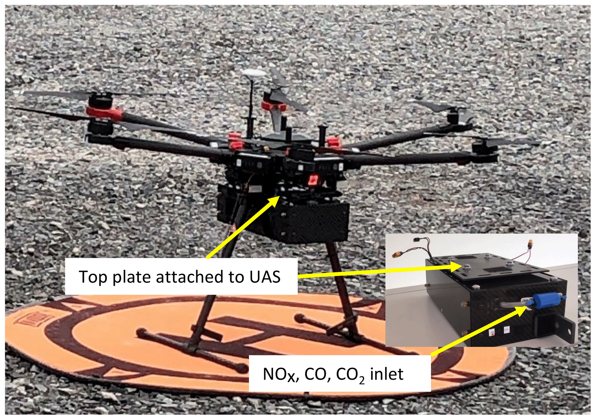
Air sampling was accomplished with an EPA–ORD-developed sensor–sampler system termed the “Kolibri”. The Kolibri consists of real-time gas sensors and pump samplers to characterize a broad range of gaseous and particle pollutants. This self-powered system has a transceiver for data transmission and pump control (Xbee S3B, Digi International, Inc., Minnetonka, MN, USA) from the ground-based operator. For this application, gas concentrations were measured using electrochemical cells for CO, NO, and NO2 and a non-dispersive infrared (NDIR) cell for CO2 (Table 1). All sensors were selected for their applicability to the anticipated operating conditions of concentration level and temperature as well as for their ability to rapidly respond to changing plume concentrations due to turbulence and entrainment of ambient air. Each sensor underwent extensive laboratory testing to verify performance and suitability prior to selection for the Kolibri. Tests included sensor performance (linearity, drift, response time, noise, detection limits) in response to anticipated field temperatures, pressure, humidity, and interferences. Additional information from the manufacturers on sensor performance is available from the links in Table 1. In anticipation of temperatures as low as 0 ∘C at the Midland site and to avoid daily temperature fluctuations, insulation was added to the Kolibri frame, and the sampled gases were preheated prior to the sensor with the use of a heating element and micro-fan inside the Kolibri. All sensors were calibrated before each sampling day under local ambient conditions. After sampling was completed, the sensors were similarly tested to assess potential drift.
Concentration data were stored by the Kolibri using a Teensy USB-based microcontroller board (Teensy 3.2, PJRC, LLC, Sherwood, OR, USA) with an Arduino-generated data program and secure digital data card. All four sensors underwent pre- and post-sampling two- or three-point calibration using gases (Calgasdirect Inc., Huntington Beach, CA, USA) traceable to National Institute of Standards and Technology (NIST) standards.
The NO sensor (NO-D4) is an electrochemical gas sensor (Alphasense, Essex, UK) that measures concentration by changes in impedance. The sensor has a detection range of 0 to 100 ppm with a resolution of < 0.1 root mean square (rms) noise (parts per million equivalent) and linearity error within ±1.5 ppm at full scale. The NO-D4 was tested to have a response time to reach 95 % of the reference concentration (t95) of 6.3 ± 0.52 s and a noise level of 0.027 ppm. The temperature and relative humidity (RH) operating range is 0 to +50 ∘C and 15 % to 90 % RH, respectively.
The NO2 sensor (NO2-D4) is an electrochemical gas sensor (Alphasense, Essex, UK) that likewise measures by impedance changes. It has an NO2 detection range of 0–10 ppm with a resolution of 0.1 rms noise (parts per million equivalent) and linearity error of 0 to 0.6 ppm at full scale. Its t95 was measured as 32.3 ± 3.8 s with a noise level of 0.015 ppm. The temperature and RH operating range is 0 to +50 ∘C and 15 % to 90 % RH, respectively.
Laboratory calibration testing prior to field measurements on both the NO-D4 and NO2-D4 sensor outputs showed their responses to be linearly proportional (R2 > 0.99) over the range of four- and five-point calibration gas concentrations. The response times of both sensors were derived using the maximum reference concentration of 47.81 ppm for NO and 10.46 ppm of NO2. The times to reach 95 % of the reference concentration, t95, were 6.3 and 32.3 s (relative standard deviation: RSD 8.2 % and 11.8 %), respectively, for the NO-D4 and NO2-D4 sensors. These response times are both shorter than those measured simultaneously in the laboratory with CEM (Ametek 9000 RM, Pittsburgh, PA, USA) at 37 and 50 s, respectively, for NO and NO2.
The CO2 sensor (CO2 Engine® K30 Fast Response, SenseAir, Delsbo, Sweden) is an NDIR gas sensor, and the voltage output is linear from 400 to 10 000 ppm. The temperature and RH operating range is 0 to +50 ∘C and 0 % to 90 % RH, respectively. The CO2-K30 sensor was measured to have a t95 response time at 6000 ppm CO2 of 9.0 ± 0.0 s and a noise level of 1.6 ppm. The response time was 4 s longer than compared to CO2 measured by a portable gas analyzer (LI-820, LI-COR Biosciences, Lincoln, NE, USA). The sensor and the LI-820 showed good agreement, as the measurements showed an R2 of 0.99 and a slope of 1.01.
The CO sensor (e2V EC4-500-CO, SGX Sensortech Ltd, High Wycombe, Buckinghamshire, UK) is described more fully elsewhere (Aurell et al., 2017; Zhou et al., 2017). In previous sensor evaluation tests with laboratory biomass burns (Zhou et al., 2017) with CO ranging between 0 and 250 ppm, the sensor was compared to simultaneous measurements by a CO continuous emission monitor (CAI model 200, California Analytical Instruments Inc., Orange, CA, USA). The concentration measurements had an R2 = 0.98 and a slope of 1.04, indicating the level of agreement between the two devices. The t90 was measured as 18 s, while the time-integrated CO concentration differences with the CAI-200, rated at t90 < 1 s, were only 4.9 %.
Variations of the Kolibri sampling system allow for measurement of additional target pollutants. These include particulate matter (PM), polycyclic aromatic hydrocarbons (PAHs), and volatile organic compounds (VOCs), including carbonyls, energetics, chlorinated organics, metals from filter analyses, and perchlorate (Aurell et al., 2017; Zhou et al., 2017).
At both facilities the aviation team from Dow flew their DJI Matrice 600 UAS, a six-motor multicopter (hexacopter), into the plumes with an EPA–ORD Kolibri sensor–sampler system attached to the undercarriage (Fig. 1). In this configuration of sensors, the Kolibri system weighed 2.4 kg. Typical flight elevations at Midland and St. Charles were 21 and 32 m above ground level (a.g.l.), respectively, and flight durations ranged from 9 to 24 min. At the St. Charles location, the UAS pilot was approximately 100 m from the center point of the two stacks, easily allowing for line-of-sight operation. A telemetry system on the Kolibri provided real-time CO2 concentration and temperature data to the Kolibri operator, who in turn advised the pilot on the optimum UAS location.
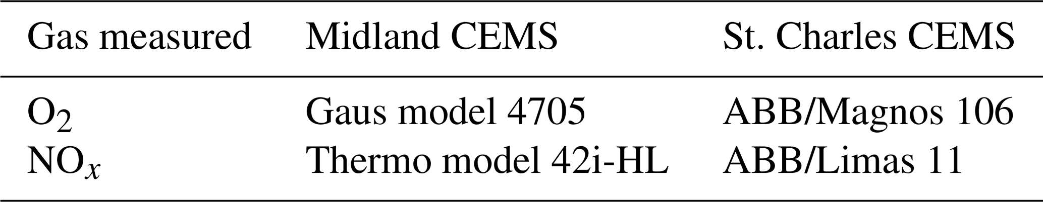
CEMSs on the boiler stacks produced a continuous record of NOx emissions and O2 concentrations. Stack and CEMS types located at the Midland and St. Charles facilities are shown in Table 2. The stack NOx analyzer uses a chemiluminescence measurement with a photomultiplier tube and is capable of split concentration range operation: low (0–180 ppm) and high (0–500 ppm). Its response time is reported as 5 s. The O2 analyzer uses a zirconium oxide cell with a measurement range of 0 % to 25 % and a reported t95 of < 10 s.
The plant CEMSs undergo annual relative accuracy audit testing (NSPS Subpart Db, Part 70) using US EPA Method 7E (2014) for NOx and US EPA Method 3A (2017) for O2. Calculation of NOx emissions uses the appropriate F factor, a value that relates the required combustion gas volume to fuel energy input, as described in US EPA Method 19 (2017). Flue gas analysis for O2 and CO2 is performed in accordance with US EPA Method 3A (2017) using an infrared analyzer to allow for calculation of the flue gas dry molecular weight.
The CEMS and UAS–Kolibri data were reduced to a common basis for comparison of results. Emission factors, or the mass of NOx per mass of fuel carbon burned, and emission rates, or the mass of NOx per energy content of the fuel, were calculated from the sample results. The determination of emission factors, defined as the mass of pollutant per mass of fuel burned, depends upon foreknowledge of the fuel composition, specifically its carbon concentration and its supply rate. The carbon in the fuel is presumed for calculation purposes to proceed to either CO2 or CO, with the minor carbon mass in hydrocarbons and PM ignored for this source type. Concurrent emission measurements of pollutant mass and carbon mass (as CO2 + CO) can be used to calculate total emissions of the pollutant from the fuel using its carbon concentration and fuel burn rate.
The UAS–Kolibri emission factors were calculated from the mass ratio of NO + NO2, with the mass of CO + CO2 resulting in a value with units of mg NOx kg−1 C. CO2 concentrations were corrected for upwind background concentrations. CEMS values of O2 and fuel flow rate were used to calculate stack flow rate using US EPA Method 19 (2017). This method requires the fuel higher heating value and an F factor (gas volume per fuel energy content, e.g., m3 kcal−1, ft3 BTU−1) to complete the calculation. For natural gas, the F factor is 967 m3 10−6 kcal (8710 ft3 10−6 BTU) (Table 19-2, US EPA Method 19, 2017). The concentration, stack flow rate, and fuel flow rate data allow for the determination of NOx and C emission rates.
The UAS–Kolibri team easily found the stack plumes at both locations using the wind direction and CO2 telemetry data transmitted to the ground operator. Use of an infrared–visible (IR: infrared) camera on a second UAS at St. Charles for some of the flights aided more rapid location of the plume and positioning of the UAS–Kolibri. Gas concentration fluctuations were rapid and of high magnitude as observed in a representative trace in Fig. 2. CO2 concentrations up to 10 000 ppm were observed; the relatively lower average CO2 concentrations reflect the rapid mixing and entrainment of ambient air, causing dilution.
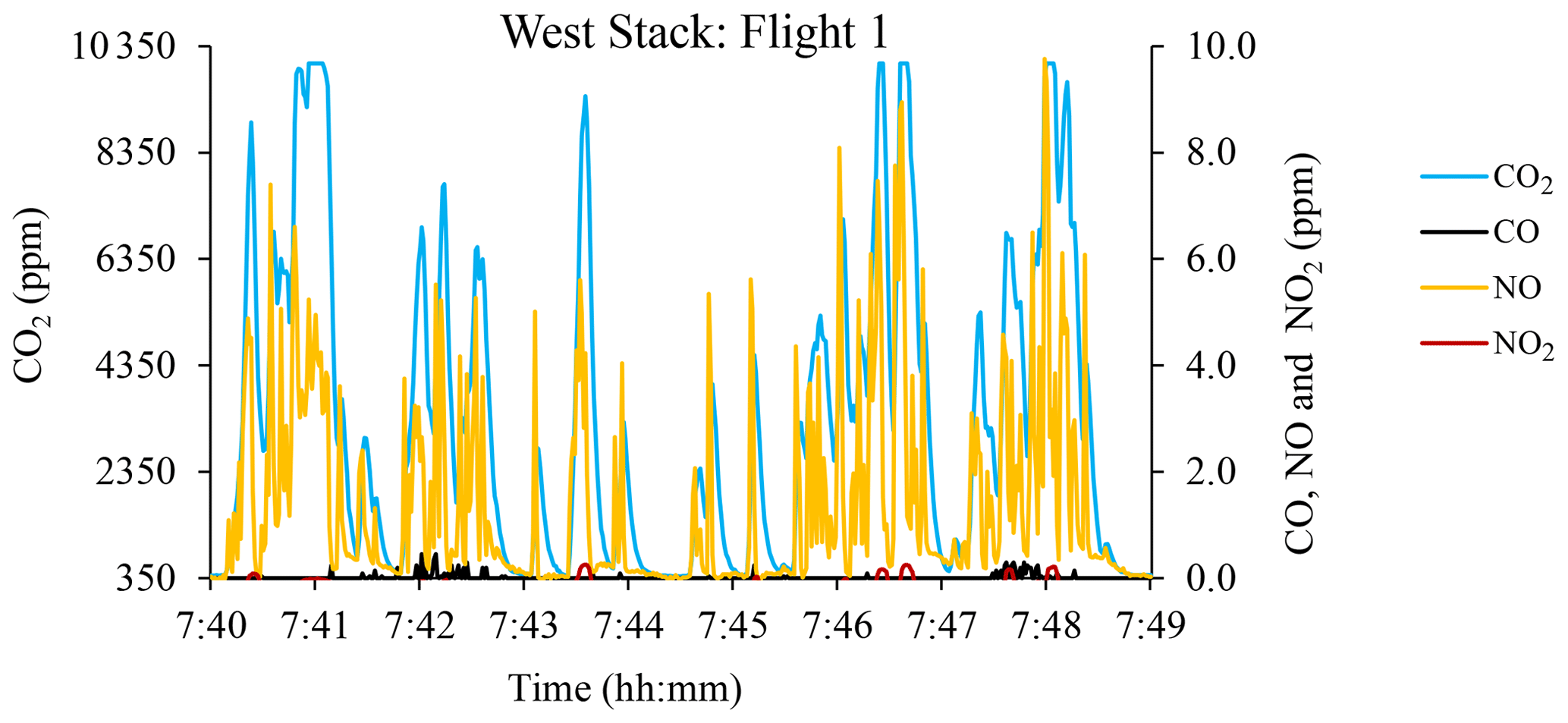
Figure 2Example of UAS–Kolibri-measured plume concentrations from the St. Charles west boiler. Data reported at 1 Hz.
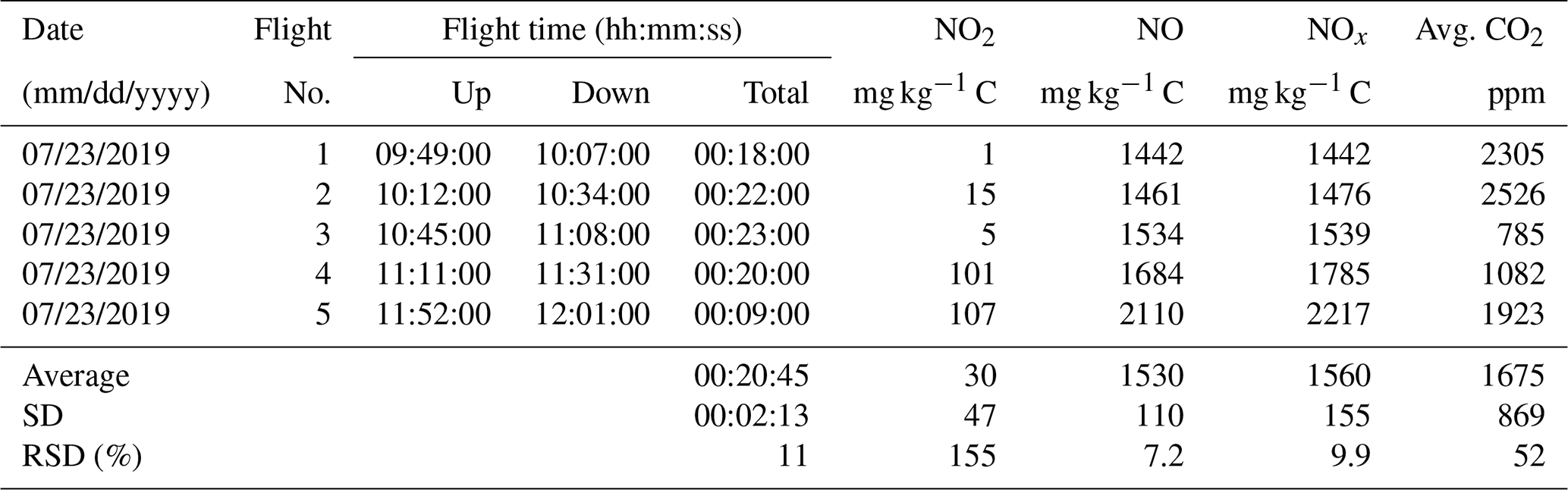
Table 3Midland UAS–Kolibri sampling data and emission factors. Time is indicated in US Central Standard Time (GMT−6).
Flight no. 4 was excluded from calculations as CO was observed, which originated from a cycling second boiler.
Table 4St. Charles east stack UAS–Kolibri sampling data and emission factors. Time is indicated in US Central Daylight Time (GMT−5).
Flight no. 5 was not included in the average as elevated CO concentrations were detected, likely from other sources in the facility.
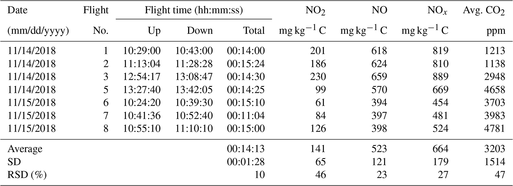
Table 5St. Charles west stack UAS–Kolibri sampling data and emission factors. Time is indicated in US Central Daylight Time (GMT−5).
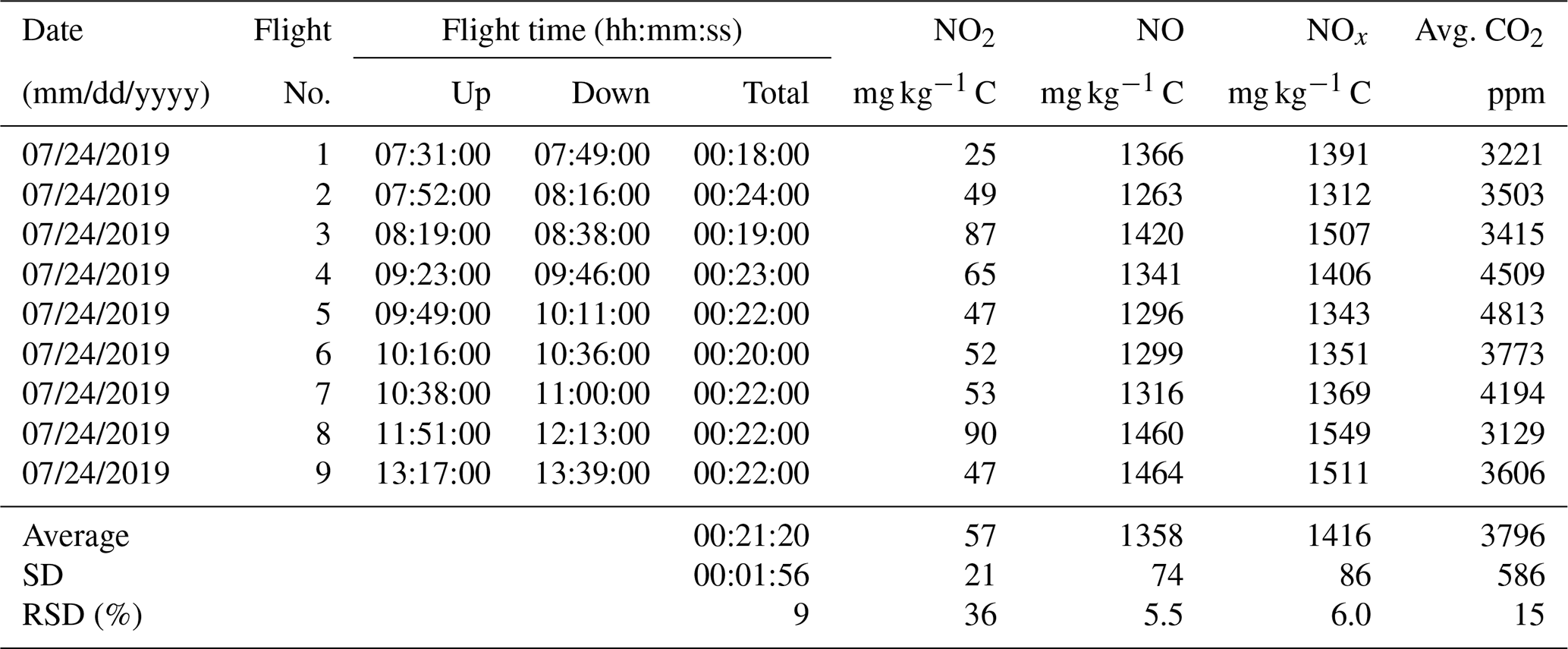
Sampling data and emission factors from the UAS–Kolibri are shown in Tables 3, 4, and 5 for the Midland, St. Charles east stack, and St. Charles west stack, respectively. Eight sampling flights were conducted at the Midland site; five were conducted on the St. Charles east boiler and nine on the St. Charles west boiler. Both boilers at the Midland site were operated under the same conditions, so their results have been presented together. Flight times averaged 14 min (10 % RSD) at the Midland facility and just over 20 min (10 % RSD) at the St. Charles facility. The shorter flight times in Midland were due to lower UAS battery capacity caused by colder temperatures (the sampling temperatures in the plume averaged 10 ± 3 ∘C). The average multi-concentration drift for each of the sensors, tested at both locations after each sampling day, was less than ±3 %. The NO2-D4 sensor showed higher drift (average 8.6 %) at one location for the highest concentration of its calibration gas (10.4 ppm). This had a minimal effect on the emission factor calibrations as the measured NO2 in the plume was actually less than 1 ppm, a range in which the drift was much lower, and NO2 is a minor contributor to the measured NOx species.
Average plume NOx concentrations were 0.88 ± 0.32 ppm at Midland and 1.22 ppm and 2.41 ppm at the two St. Charles boilers, with an average RSD of 37 %, 36 %, and 12 %, respectively. The NO emission factor was typically 97 % of the total NOx, with the NO2 providing the minor balance.

Table 6 presents the average O2 and NOx measurement results and the fuel supply rate at both locations. Values for natural gas supply, adjusted for the C2H6 and H2 composition of the St. Charles fuel, were used to calculate the fuel carbon supply rate. These data allow for the calculation of the emission factor, or the mass of NOx to the mass of carbon, which is reported in Table 7.
Table 7Comparison of average NOx emission factors from CEMS and UAS–Kolibri.
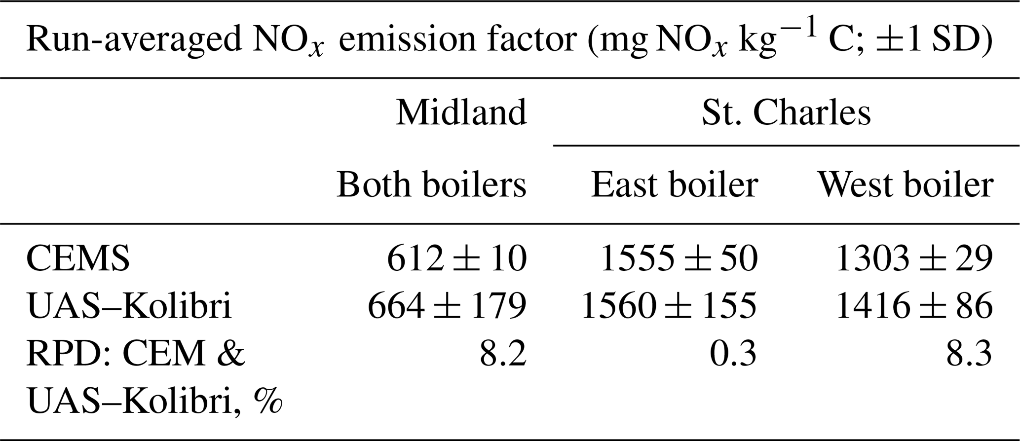
The UAS–Kolibri NOx emission factor for Midland is 8 % higher than the simultaneous CEMS value. For the east and west boilers at St. Charles, the UAS–Kolibri NOx emission factor value is < 1 % and 8 % higher, respectively, than the CEMS values. The difference for the UAS–Kolibri in Midland may be attributed in part to the extremely cold temperature affecting the performance of the electrochemical sensors. The standard deviations for the CEMS data are based on the run-averaged NOx values for each test. These values were calculated based on 10 s averaging for the Midland tests, 60 s averaging in St. Charles, and 1 s averaging for the UAS–Kolibri. Higher standard deviations for the UAS–Kolibri are predictable given the rapidly changing values and wide range (∼ 0–10 ppm) of NOx data observed in Fig. 2. Difference testing for the CEMS and UAS–Kolibri using α = 0.05 and assumed unequal variances indicates that only the west boiler and UAS–Kolibri are statistically distinct.
The emission rates calculated from the UAS–Kolibri data are 5.6, 14.6, and 13.3 kg NOx × 10−3 kJ (0.013, 0.034, and 0.031 lb NOx × 10−6 BTU), respectively, for the Midland, east St. Charles, and west St. Charles boilers, which are below the regulatory standard of 15.5 kg NOx × 10−3 kJ (0.036 lb NOx × 10−6 BTU). The emission factors were also calculated as carbon-weighted values to reflect potential differences in plume sampling efficiency between runs. The Midland, east St. Charles, and west St. Charles UAS–Kolibri emission factors were 607, 1525, and 1409 mg NOx kg−1 C, respectively. These amounted to relative percent differences of 0.8 %, 1.9 %, and 7.8 % between the CEM and UAS–Kolibri values for an overall run-weighted average difference of 5.6 %. The difference between the CEM readings and those from the Kolibri weighted by the carbon collection amounts, reflecting success at being within the higher plume concentrations, was 3.5 %.
This work reports, to our knowledge, the first known comparison of continuous emission monitoring measurements made in a stack to downwind plume measurements made using a UAS equipped with emission sensors.
The UAS–Kolibri system was easily able to find and take measurements from the downwind plume of a natural gas boiler despite the lack of any visible plume signature. The telemetry system aboard the Kolibri reported real-time CO2 concentrations to the operator on the ground, allowing the operator to provide immediate feedback to the UAS pilot on plume location. Comparison of the CEM data to the UAS–Kolibri data from field measurements at two locations showed agreement of NOx emission factors within 5.6 % and 3.5 % for time-weighted and carbon-collection-weighted measurements, respectively. This work demonstrates the accuracy of a UAS-borne emission sampling system for quantifying point source strength. These results also have applicability to area source measurements, such as open fires, which similarly employ the carbon balance method to determine source strength emission factors.
Data are available from the Environmental Dataset Gateway (https://edg.epa.gov/metadata/catalog/main/home.page, last access: 27 January 2021; https://doi.org/10.23719/1520733, Gullett, 2021) and the authors upon request. The raw, primary data on sensor voltages are processed to concentration values through time synchronization of data and user-defined, customized scripts for calibration that are a function of the gas sensor type and site-specific temperature, pressure, and relative humidity. Interested parties are welcome to contact the corresponding author for recommendations on how to customize this process to fit their specific scenarios.
BG was the prime author of the paper and the project lead. JA conducted the Kolibri field testing and data analysis. WM designed the instrument electronics. JR led the UAS group and field test arrangements.
The authors declare that they have no conflict of interest.
The views expressed in this article are those of the authors and do not necessarily represent the views or policies of the U.S. EPA.
Dow's Corporate Aviation Group includes Laine Miller, Bryce Young, James Waddell, Jeffrey Matthews, Chris Simmons, and Anthony DiBiase, who conducted flights flawlessly. Dow employees Rob Seibert and Alex Kidd provided technical data, and Amy Meskill (Dow), Jennifer DeMelo (Dow), and Dale Greenwell (EPA–ORD) provided critical logistic support. Patrick Clark (Montrose) reviewed the St. Charles CEMS data.
This research has been supported by the Dow Chemical Company through a Cooperative Research and Development Agreement with the US Environmental Protection Agency.
This paper was edited by Michel Van Roozendael and reviewed by two anonymous referees.
Aurell, J., Mitchell, W., Chirayath, V., Jonsson, J., Tabor, D., and Gullett, B.: Field determination of multipollutant, open area combustion source emission factors with a hexacopter unmanned aerial vehicle, Atmos. Environ., 166, 433–440, https://doi.org/10.1016/j.atmosenv.2017.07.046, 2017.
Brady, J. M., Stokes, M. D., Bonnardel, J., and Bertram, T. H.: Characterization of a Quadrotor Unmanned Aircraft System for Aerosol-Particle-Concentration Measurements, Environ. Sci. Technol., 50, 1376–1383, https://doi.org/10.1021/acs.est.5b05320, 2016.
Chang, C.-C., Wang, J.-L., Chang, C.-Y., Liang, M.-C., and Lin, M.-R.: Development of a multicopter-carried whole air sampling apparatus and its applications in environmental studies, Chemosphere, 144, 484–492, https://doi.org/10.1016/j.chemosphere.2015.08.028, 2016.
Craft, T. L., Cahill, C. F., and Walker, G. W.: Using an Unmanned Aircraft to Observe Black Carbon Aerosols During a Prescribed Fire at the RxCADRE Campaign, 2014 International Conference on Unmanned Aircraft Systems, 27–30 May 2014, Orlando, FL, USA, 2014.
Gullett, B.: Dow UAS NOx Stack Boiler Emissions [Data set], U.S. EPA Office of Research and Development (ORD), https://doi.org/10.23719/1520733, 2021.
Li, X. B., Wang, D. F., Lu, Q. C., Peng, Z. R., Fu, Q. Y., Hu, X. M., Huo, J. T., Xiu, G. L., Li, B., Li, C., Wang, D. S., and Wang, H. Y.: Three-dimensional analysis of ozone and PM2.5 distributions obtained by observations of tethered balloon and unmanned aerial vehicle in Shanghai, China, Stoch. Env. Res. Risk A., 32, 1189–1203, https://doi.org/10.1007/s00477-018-1524-2, 2018.
Mori, T., Hashimoto, T., Terada, A., Yoshimoto, M., Kazahaya, R., Shinohara, H., and Tanaka, R.: Volcanic plume measurements using a UAV for the 2014 Mt. Ontake eruption, Earth Planets Space, 68, 49, https://doi.org/10.1186/s40623-016-0418-0, 2016.
Neumann, P. P., Bennetts, V. H., Lilienthal, A. J., Bartholmai, M., and Schiller, J. H.: Gas source localization with a micro-drone using bio-inspired and particle filter-based algorithms, Adv. Robotics, 27, 725–738, https://doi.org/10.1080/01691864.2013.779052, 2013.
Peng, Z.-R., Wang, D., Wang, Z., Gao, Y., and Lu, S.: A study of vertical distribution patterns of PM2.5 concentrations based on ambient monitoring with unmanned aerial vehicles: A case in Hangzhou, China, Atmos. Environ., 123, 357–369, https://doi.org/10.1016/j.atmosenv.2015.10.074, 2015.
Rosser, K., Pavey, K., FitzGerald, N., Fatiaki, A., Neumann, D., Carr, D., Hanlon, B., and Chahl, J.: Autonomous Chemical Vapour Detection by Micro UAV, Remote Sens., 7, 16865–16882, https://doi.org/10.3390/rs71215858, 2015.
U.S. EPA Method 7E: Determination of Nitrogen Oxides Emissions from Stationary Sources (Instrumental Analyzer Procedure), available at: https://www.epa.gov/sites/production/files/2016-06/documents/method7e.pdf (last access: 7 August 2019), 2014.
U.S. EPA Method 3A: Determination of oxygen and carbon dioxide concentrations in emissions from stationary sources (instrumental analyzer procedure), available at: https://www.epa.gov/sites/production/files/2017-08/documents/method_3a.pdf (last access: 12 February 2019), 2017.
U.S. EPA Method 19: Determination of sulfur dioxide removal efficiency and particulate matter, sulfur dioxide, and nitorgen oxide emission rates, available at: https://www.epa.gov/sites/production/files/2017-08/documents/method_19.pdf (last access: 6 December 2018), 2017.
Villa, T. F., Salimi, F., Morton, K., Morawska, L., and Gonzalez, F.: Development and Validation of a UAV Based System for Air Pollution Measurements, Sensors, 16, 12, https://doi.org/10.3390/s16122202, 2016.
Zhou, X., Aurell, J., Mitchell, W., Tabor, D., and Gullett, B.: A small, lightweight multipollutant sensor system for ground-mobile and aerial emission sampling from open area sources, Atmos. Environ., 154, 31–41, https://doi.org/10.1016/j.atmosenv.2017.01.029, 2017.